appendix b a biologist’s introduction to spectrum analysis

Appendix B A Biologist’s Introduction toSpectrum Analysis

About this appendix

This appendix provides some conceptual background for making and interpreting spectrogram and spectrogram slice views with Raven. It introduces the short-time Fourier transform (STFT), the mathematical technique used by Raven for making spectrograms. We do not discuss the mathematics of the STFT, but instead treat it here as a black box. This black box has controls on its outside that affect its operation in important ways. One aim of this appendix is to convey enough qualitative understanding of the behavior of this box to allow intelligent use of its controls, without delving into the box’s internal mechanism. Specific details of the controls are covered in Chapter 3, “Spectrographic Analysis”. A second aim of this appendix is to explain some of the limitations and tradeoffs intrinsic to spectrum analysis of time-varying signals. More rigorous mathematical treatments of spectral analysis, at several levels of sophistication, can be found in the references listed at the end of the appendix.

Several approaches can be taken to explaining the fundamentals of digital spectrum analysis. The approach taken in this appendix is geared specifically to spectrum analysis with Raven; thus some of the terms and concepts used here may not appear in other, more general discussions of spectrum analysis, such as those listed at the end of the appendix.

The discussions in this appendix assume a basic understanding of how sound is recorded and represented digitally. If you are not already acquainted with concepts such as sample rate and sample size, you should read Appendix A, “Digital Representation of Sound” before proceeding.

What sound is

Sound consists of traveling waves of alternating compression and rarefaction in an elastic medium (such as air or water), generated by some vibrating object (a sound source).

Sound pressure is the (usually small) alternating incremental change in pressure from ambient pressure that results from a sound. When no sound is present in a medium (i.e., there is no propagating pressure change), we say that sound pressure is zero, even though the medium does exert some static ambient pressure. The dimensions of pressure are force per unit

Raven Pro 1.4 User’s Manual 327

Appendix B: A Biologist’s Introduction to Spectrum Analysis

area. The usual unit of sound pressure is the pascal (abbreviated Pa); one pascal equals one newton per square meter. Since the smallest audible sound pressures in air are on the order of 10-6 Pa, sound pressures are usually expressed in µPa.

To measure or record sound at a particular location in space, we use a device such as a microphone that responds to sound pressure. A microphone produces a time-varying electrical voltage that is proportional to the increase or decrease in local pressure that constitutes sound. This continuous time-varying voltage is an electric analog of the acoustic signal. The continuous electric signal can be converted to a digital representation suitable for manipulation by a computer as discussed in Appendix A, “Digital Representation of Sound”.

Time domain and frequency domain representations of sound

Any acoustic signal can be graphically or mathematically depicted in either of two forms, called the time domain and frequency domain representations. In the time domain, instantaneous pressure is represented as a function of time. Figure B.1a shows the time domain representation of the simplest type of acoustic signal, a pure tone. Such a signal is called a sinusoid because its amplitude is a sine function of time, characterized by some frequency, which is measured in cycles per second, or Hertz (Hz). The frequency of a sinusoid is most easily determined by measuring the length of one period, which is the reciprocal of the frequency. The amplitude of the signal in the time domain is measured in pressure units. (Once an acoustic signal has been converted by a microphone into an electrical signal, amplitude is measured as voltage, which is directly proportional to the sound pressure.) In the frequency domain, the amplitude of a signal is represented as a function of frequency. The frequency domain representation of a pure tone is a vertical line (Figure B.1b).

328 Raven Pro 1.4 User’s Manual


Figure B.1. Time and freq domain

Figure B.1. Time domain and frequency domain representations of an infinitely long pure sinusoidal signal. (a) Time domain. t is the period of the sinusoid. (b) Frequency domain. f is the frequency of the sinusoid.

Any sound, no matter how complex, can be represented as the sum of a series of pure tones (sinusoidal components). Each tone in the series has a particular amplitude, and a particular phase relationship (i.e., it may be shifted in time) relative to the others. The frequency composition of complex signals is usually not apparent from inspection of the time domain representation. Spectrum analysis is the process of converting the time domain representation of a signal to a frequency domain representation that shows how different frequency components contribute to the sound. Frequency domain representations of sounds are often more intuitively interpretable because the mammalian auditory system (specifically the cochlea) performs a type of spectrum analysis in converting vibrations of the eardrum into neural impulses. Our auditory perception is thus based on a frequency domain representation of sounds.

The complete frequency domain representation of a signal consists of two parts. The magnitude spectrum (Figure B.2b) contains information about the relative magnitude of each frequency component in the entire signal. The phase spectrum (Figure B.2c) contains information about the relative phase or timing relationships among the frequency components. Since the phase spectrum is rarely of practical use in most bioacoustic work and is not provided by Raven, it is not discussed further here. Henceforth, unless



otherwise noted, we use the term “spectrum” to refer to the magnitude spectrum alone.

Figure B.2. Time, freq domains-- 2 tones

Figure B.2. Time domain and frequency domain representations of an infinitely long sound consisting of two tones, with frequencies of 490 Hz and 800 Hz. (a) Time domain. (b) Magnitude spectrum in frequency domain. (c) Phase spectrum in frequency domain. The phase of the frequency component at 500 Hz is arbitrarily taken as a reference and assigned a phase value of 0.

The Fourier transform is a mathematical function that converts the time domain form of a signal (which is the representation directly produced by most measuring and recording devices) to a frequency domain representation, or spectrum. When the signal and spectrum are represented as a sequence of discrete digital values, a version of the Fourier transform called the discrete Fourier transform (DFT) is used. The



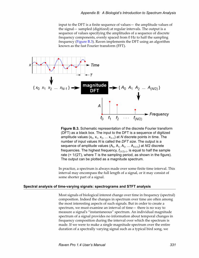
input to the DFT is a finite sequence of values— the amplitude values of the signal— sampled (digitized) at regular intervals. The output is a sequence of values specifying the amplitudes of a sequence of discrete frequency components, evenly spaced from 0 Hz to half the sampling frequency (Figure B.3). Raven implements the DFT using an algorithm known as the fast Fourier transform (FFT).

Figure B.3. DFT schematic

Figure B.3. Schematic representation of the discrete Fourier transform (DFT) as a black box. The input to the DFT is a sequence of digitized amplitude values (x0, x1, x2, ... xN-1) at N discrete points in time. The number of input values N is called the DFT size. The output is a sequence of amplitude values (A0, A1, A2, ... A(N/2)) at N/2 discrete frequencies. The highest frequency, f(N/2)-1, is equal to half the sample rate (= 1/(2T), where T is the sampling period, as shown in the figure). The output can be plotted as a magnitude spectrum.

In practice, a spectrum is always made over some finite time interval. This interval may encompass the full length of a signal, or it may consist of some shorter part of a signal.

Spectral analysis of time-varying signals: spectrograms and STFT analysis

Most signals of biological interest change over time in frequency (spectral) composition. Indeed the changes in spectrum over time are often among the most interesting aspects of such signals. But in order to create a spectrum, we must examine an interval of time— there is no way to measure a signal’s “instantaneous” spectrum. An individual magnitude spectrum of a signal provides no information about temporal changes in frequency composition during the interval over which the spectrum is made. If we were to make a single magnitude spectrum over the entire duration of a spectrally varying signal such as a typical bird song, we



would have a representation of the relative intensities of the various frequency components of the signal, but we would have no information about how the intensities of different frequencies varied over time during the signal.

To see how the frequency composition of a signal changes over time, we can examine a sound spectrogram.1 The spectrograms produced by Raven plot frequency on the vertical axis versus time on the horizontal; the amplitude of a given frequency component at a given time is represented by a color (by default, grayscale) value (Figure B.4).

Figure B.4. Spectrogram example.

Figure B.4. Smoothed sound spectrogram of part of a song of a chestnut-sided warbler, digitized at 44.1 kHz.

Spectrograms are produced by a procedure known as the short-time Fourier transform (STFT). The STFT divides the entire signal into a series of successive short time segments, called records (or frames). Each record is used as the input to a DFT, generating a series of spectra (one for each record). To display a spectrogram, the spectra of successive records are plotted side by side with frequency running vertically and amplitude at each frequency represented by a color (by default, grayscale) value. Raven’s spectrogram slice view displays the spectrum of one record at a time as a line graph, with frequency on the horizontal axis, and amplitude on the vertical axis. A spectrogram can be characterized by its DFT size, expressed as the number of digitized amplitude samples that are processed to create each individual spectrum.

The STFT can be considered as equivalent in function to a bank of N/2 + 1 bandpass filters, where N is the DFT size. Each filter is centered at a slightly different analysis frequency. The output amplitude of each filter is proportional to the amplitude of the signal in a discrete frequency band or bin, centered on the analysis frequency of the filter. In this “filterbank” model of STFT analysis, the spectrogram is considered as representing the

1. Sound spectrograms are sometimes called sonagrams. Strictly speaking, how-ever, the term sonagram is a trademark for a sound spectrogram produced by a particular type of spectrum analysis machine called a Sonagraph, produced by the Kay Elemetrics Co.



time-varying output amplitudes of filters at successive analysis frequencies plotted above each other, with amplitude again represented by color (by default, grayscale) values. A spectrogram can be characterized by its bandwidth, the range of input frequencies around the central analysis frequency that are passed by each filter. All of the filters in a spectrogram have the same bandwidth, irrespective of analysis frequency.

Record length, bandwidth, and the time-frequency uncertainty principle

The record length of a STFT determines the time analysis resolution (Δt) of the spectrogram. Changes in the signal that occur within one record (e.g., the end of one sound and the beginning of another, or changes in frequency) cannot be resolved as separate events. Thus, shorter record lengths allow better time analysis resolution.

Similarly, the bandwidth of a STFT determines the frequency analysis resolution (Δf) of the spectrogram: frequency components that differ by less than one filter-bandwidth cannot be distinguished from each other in the output of the filterbank. Thus a STFT with a relatively wide bandwidth will have poorer frequency analysis resolution than one with a narrower bandwidth.

Ideally we might like to have very fine time and frequency analysis resolution in a spectrogram. These two demands are intrinsically incompatible, however: the record length and filter bandwidth of a STFT are inversely proportional to each other, and cannot be varied independently. Although a short record length yields a spectrogram with finer time analysis resolution, it also results in wide bandwidth filters and correspondingly poor frequency analysis resolution. Thus a tradeoff exists between how precisely a spectrogram can specify the spectral (frequency) composition of a signal and how precisely it can specify the time at which the signal exhibited that particular spectrum.

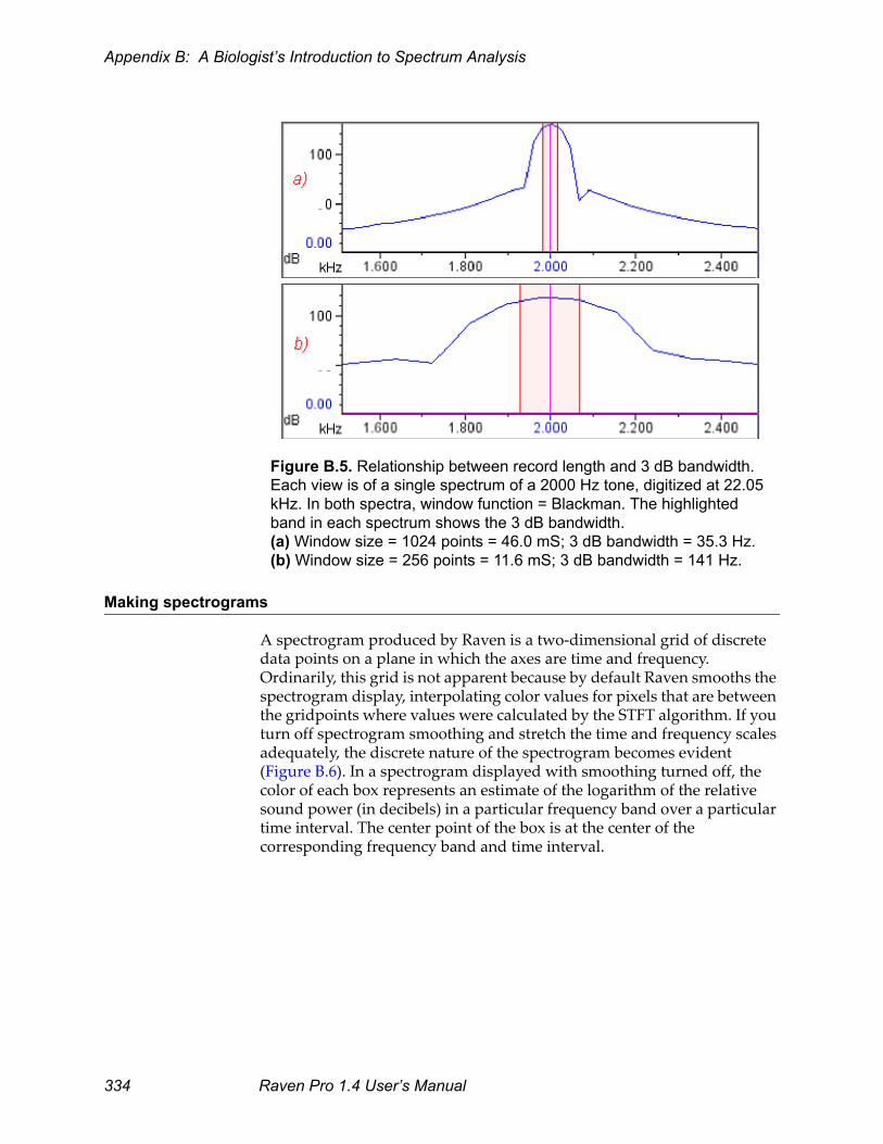
The relationship between record length and filter bandwidth applies to each of the individual spectra that collectively constitute a spectrogram. Figure B.5 illustrates the relationship between record length and filter bandwidth in individual spectra. The two spectra, of a 2000 Hz pure tone digitized at 22.05 kHz, were made with different record lengths and thus different bandwidths. Spectrum (a), with a record length of 1024 points (46.0 mS), shows a fairly sharp peak at 2000 Hz because of its relatively narrow bandwidth (35.3 Hz) filter; spectrum (b), with a record length of 256 points (11.5 mS), corresponding to a wider bandwidth (141 Hz) filter, has poorer frequency resolution.



Figure B.5. Window length - bandwidth relationship

Figure B.5. Relationship between record length and 3 dB bandwidth. Each view is of a single spectrum of a 2000 Hz tone, digitized at 22.05 kHz. In both spectra, window function = Blackman. The highlighted band in each spectrum shows the 3 dB bandwidth.(a) Window size = 1024 points = 46.0 mS; 3 dB bandwidth = 35.3 Hz.(b) Window size = 256 points = 11.6 mS; 3 dB bandwidth = 141 Hz.

Making spectrograms

A spectrogram produced by Raven is a two-dimensional grid of discrete data points on a plane in which the axes are time and frequency. Ordinarily, this grid is not apparent because by default Raven smooths the spectrogram display, interpolating color values for pixels that are between the gridpoints where values were calculated by the STFT algorithm. If you turn off spectrogram smoothing and stretch the time and frequency scales adequately, the discrete nature of the spectrogram becomes evident (Figure B.6). In a spectrogram displayed with smoothing turned off, the color of each box represents an estimate of the logarithm of the relative sound power (in decibels) in a particular frequency band over a particular time interval. The center point of the box is at the center of the corresponding frequency band and time interval.



Figure B.6. Boxy spectrogram

Figure B.6. Same spectrogram as in Figure B.4, with smoothing turned off. The grayscale value in each box represents an estimate of the relative power in the corresponding frequency band and time interval. Filter bandwidth = 124 Hz, window size (record length) = 512 samples (= 11.6 mS). Grid spacing = 5.8 mS x 86.1 Hz.

Raven lets you specify the spacing between gridpoints in the time dimension and thus the width of the boxes in an unsmoothed spectrogram. In Raven’s Configure Spectrogram dialog, you can specify the time grid spacing (also called hop size) directly, or indirectly by specifying the amount of overlap between successive records. (You specify the record length of a spectrogram in Raven by entering the size of a window function. Window functions are discussed in “Window functions” on page 342.) The spacing between gridpoints in the frequency dimension is determined by the DFT size. Raven chooses DFT size automatically, using the smallest power of 2 which is greater than or equal to the window size (in samples).

The relationships between time grid spacing and record overlap, and between frequency grid spacing and DFT size are discussed below. See Chapter 5, “Spectrographic Analysis”, for a detailed discussion of how to control these parameters in Raven.

Grid spacing should not be confused with analysis resolution. Analysis resolution for time and frequency are determined by the record length and bandwidth of a STFT, respectively. Analysis resolution describes the amount of smearing or blurring of temporal and frequency structure at each point on the grid, irrespective of the spacing between these points. The following sections seek to clarify the concepts of analysis resolution and grid spacing by showing examples of spectrograms that illustrate the difference between the two.

Analysis resolutionand the time-

frequencyuncertainty

principle

At each point on the spectrogram grid, the tradeoff between time and frequency analysis resolution is determined by the relationship between record length and bandwidth, as discussed above. According to the uncertainty principle, a spectrogram can never have extremely fine analysis resolution in both the frequency and time dimensions.



For example, Figure B.7 shows two spectrograms of the same signal that differ in record length and hence, bandwidth. In spectrogram (a), with a record length of 64 points (= 2.9 mS; bandwidth = 496 Hz), the beginning and end of each tone can be clearly distinguished and are well-aligned with the corresponding features of the waveform. However, the frequency analysis resolution is poor: each tone appears as a bar that is nearly 1200 Hz in thickness. In spectrogram (c), the record length is 512 points, or 23 mS (filter bandwidth = 61.9 Hz), or about as long as each tone in the signal. Most of the records therefore span more than one tone, in some cases including a tone and a silent interval, in other cases including two tones and an interval. The result is poor time resolution: the beginning and end of the bars representing the tones are fuzzy and poorly aligned with features of the waveform (compare, for example, the beginning time of the first pulse in the waveform with the corresponding bar in the spectrogram). However, this spectrogram has much better frequency resolution than spectrogram (a): the bar representing each tone is only about 100 Hz in thickness.



Figure B.7. Time vs freq resolution.

Figure B.7. Effect of record length and filter bandwidth on time and frequency resolution. The signal consists of a sequence of four tones with frequencies of 1, 2, 3, and 4 kHz, at a sample rate of 22.05 kHz. Each tone is 20 mS in duration. The interval between tones is 10 mS. Both spectrograms have the same time grid spacing = 1.45 mS, and window function = Hann. The selection boundaries show the start and end of the second tone.(a) Wide-band spectrogram: record length = 64 points ( = 2.90 mS), 3 dB bandwidth = 496 Hz.(b) Waveform, showing timing of the tones.(c) Narrow-band spectrogram: record length = 512 points ( = 23.2 mS), 3 dB bandwidth = 61.9 Hz.The waveform between the spectrograms shows the timing of the pulses.

What is the “best” window size to choose? The answer depends on how rapidly the signal’s frequency spectrum changes, and on what type of information is most important to show in the spectrogram, given your particular application. For many applications, Raven’s default window size (512 samples) provides a reasonable balance between time and frequency resolution. If you need to observe very short events or rapid changes in the signal, a shorter window may be better; if precise frequency representation is more important, a longer window may be better2. If you need better time and frequency resolution than you can achieve in one

2. If the features that you’re interested in are distinguishable in the waveform (e.g., the beginning or end of a sound, or some other rapid change in ampli-tude), you’ll achieve better precision and accuracy by making time measure-ments on the waveform rather than the spectrogram.



spectrogram, you may need to make two spectrograms: a wide-band spectrogram with a small window for making precise time measurements, and a narrow-band spectrogram with a larger window for precise frequency measurements.

Time grid spacingand window overlap

Time grid spacing (also called hop size) is the time between the beginnings of successive records. In an unsmoothed spectrogram, this interval is visible as the width of the individual boxes (Figure B.6). Successive records that are analyzed may be overlapping (positive overlap), contiguous (zero overlap), or discontiguous (negative overlap). Overlap between records is usually expressed as a percentage of the record length.

Figure B.8 illustrates the different effects of changes to record length and time grid spacing. The signal is a frequency-modulated tone that sweeps upward in frequency from 4 to 6 kHz, sampled at 22.05 kHz. Spectrograms (a) and (c) both have a record length of 512 points (= 23.2 mS; 3 dB bandwidth = 61.9 Hz). (a) was made with 0% overlap (time grid spacing = 23.2 mS), whereas (c) was made with an overlap of 93.8% (time grid spacing = 1.45 mS). In the low-resolution spectrogram (a), each box is as wide as one data record, which in turn is one quarter of the length of the tone. The result is a spectrogram that gives an extremely misleading picture of the signal. Spectrogram (c), with a greater record overlap, is much “smoother” than the one with less overlap, and it more accurately portrays the continuous frequency modulation of the signal. It still provides poor time analysis resolution, however, because of its large record length— notice the fuzzy beginning and end of the spectrogram image of the tone and the poor alignment with the beginning and end of the tone in the waveform. Comparison of the spectrograms in Figure B.8 demonstrates that improved time grid spacing is not a substitute for finer time analysis resolution, which can be obtained only by using a shorter record.



Figure B.8. Window size window size - overlap

Figure B.8. Different effects on spectrograms of changing record length (= window size, or time analysis resolution) and time grid spacing. The signal is a frequency-modulated tone, 100 mS long, sampled at 22.05 kHz. The tone sweeps upward in frequency from 4 to 6 kHz. Spectrograms (a) and (c) have the same window size, but (c) has finer time grid spacing (higher record overlap). (c) and (d) have the same time grid spacing, but (d) has a shorter record length (finer time analysis resolution).(a) Record length = 512 points = 23.2 mS (3 dB bandwidth = 61.9 Hz);Time grid spacing = 23.2 mS (overlap = 0%).(b) Waveform view, with duration of tone highlighted. (c) Record length = 512 points = 23.2 mS (3 dB bandwidth = 61.9 Hz);Time grid spacing = 1.45 mS (overlap = 93.8%).(d) Record length = 64 points = 2.9 mS (3 dB bandwidth = 448 Hz);Time grid spacing = 1.45 mS (overlap = 50%).

Frequency gridspacing and DFT

size

Frequency grid spacing is the difference (in Hz) between the central analysis frequencies of adjacent filters in the filterbank modeled by a STFT, and thus the size of the frequency bins in a spectrogram. In an unsmoothed spectrogram, this spacing is visible as the height of the individual boxes (Figure B.6). Frequency grid spacing depends on the sample rate (which is fixed for a given digitized signal) and DFT size. The relationship is

frequency grid spacing = (sample rate) / DFT size



where frequency grid spacing and sample rate are measured in Hz, and DFT size is measured in samples. Thus a larger DFT size draws the spectrogram on a grid with finer frequency resolution (smaller frequency bins, vertically smaller boxes). The number of frequency bins in a spectrogram or spectrum is half the DFT size, plus one.

Recall that the DFT size is the number of samples processed to calculate the spectrum of a record. Thus the DFT size would ordinarily be equal to the record length. However, Raven’s DFT algorithm requires that the size of the DFT be a power of 2. Therefore Raven automatically chooses the smallest DFT size that is a power of 2 greater than or equal to the record size. The sample data in each record are then filled out with zeros (“zero-padded”) to make the record length the same as the chosen DFT size. Zero padding provides the right number of samples to match the chosen DFT size without altering the spectrum of the data.

Spectral smearingand sidelobes

The spectra that constitute a spectrogram produced by a STFT are “imperfect” in several respects. First, as discussed above, each filter simulated by the STFT has a finite band of frequencies to which it responds; the filter is unable to discriminate different frequencies within this band. According to the uncertainty principle, the filter bandwidth can be reduced— thus improving frequency resolution— only by analyzing a longer record, which reduces temporal resolution.

Second, the passbands of adjacent filters overlap in frequency, so that some frequencies are passed (though partially attenuated) by more than one filter (Figure B.9). Consequently, when a spectrum or spectrogram is constructed by plotting the output of all of the filters, a signal consisting of a pure tone becomes “smeared” in frequency (Figure B.9d).



Figure B.9. Spectral smearing-- overlapping filters

Figure B.9. Spectral smearing resulting from overlapping bandpass filters. (a) A single hypothetical bandpass filter centered at frequency f0. When the input to the filter is a pure tone at frequency f0, the output amplitude is A0. For clarity of illustration, sidelobes to the main passband are not shown (see text and Figure B.10). (b) Two overlapping filters, centered at frequencies f0 and f1. When the filter centered at f1 is presented with the same input as in (a), its output amplitude is A1. (c) A bank of overlapping filters simulated by a STFT. Frequency f0 falls within the passbands of the filter centered at f0, and of two filters (blue and green) on either side. (d) Spectrum of a pure tone signal of frequency f0 produced by the filterbank shown in (c). The spectrum consists of one amplitude value from each filter. Because the filters overlap, the spectrum is smeared, showing energy at frequencies adjacent to f0. The shape of the resulting spectrum is the same as that of a single filter.



Third, each filter does not completely block the passage of all frequencies outside of its nominal passband. For each filter there is an infinite series of diminishing sidelobes in the filter’s response to frequencies above and below the passband (Figure B.10). These sidelobes arise because of the onset and termination of the portion of the signal that appears in a single record. Since a spectrum of a pure tone made by passing the tone through a set of bandpass filters resembles the frequency response of a single filter (Figure B.9), a STFT spectrum of any signal (even a pure tone) contains sidelobes.

Figure B.10. Filter sidelobes

Figure B.10. Frequency response of a hypothetical bandpass filter from a set of filters simulated by a short-time Fourier transform, showing sidelobes above and below the central lobe, or passband. The magnitude of the sidelobes relative to the central lobe can be reduced by use of a window function (see text). Note that a spectrum produced by passing a pure tone through a set of overlapping filters is shaped like the frequency response of a single one of the filters (see Figure B.9).

Window functions The magnitude of the sidelobes (relative to the magnitude of the central lobe) in a spectrogram or spectrum of a pure tone is related to how abruptly the windowed signal’s amplitude changes at the beginning and end of a record. A sinusoidal tone that instantly rises to its full amplitude at the beginning of a record, and then instantly falls to zero at the end, has higher sidelobes than a tone that rises and falls gradually in amplitude (Figure B.11).



Figure B.11. Windowing

Figure B.11. Relationship between abruptness of onset and termination of signal in one record and spectral sidelobes. Each panel shows a signal on the left, and its spectrum on the right.(a) A single record of an untapered sinusoidal signal has a spectrum that contains a band of energy around the central frequency, flanked by sidelobes, as if the signal had been passed through a bank of bandpass filters like the one shown in Figure B.10.(b) A single record of a sinusoidal signal multiplied by a “taper” or window function, has smaller sidelobes.

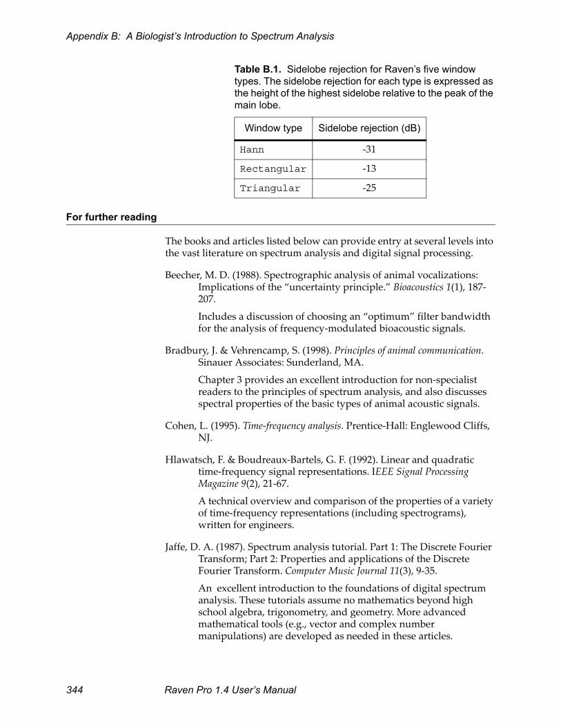
The magnitude of the sidelobes in a spectrum or spectrogram can be reduced by multiplying the record by a window function that tapers the waveform as shown in Figure B.11. Tapering the waveform in the record is equivalent to changing the shape of the analysis filter (in particular, lowering its sidelobes). Each window function reduces the height of the highest sidelobe to some particular proportion of the height of the central peak; this reduction in sidelobe magnitude is termed the sidelobe rejection, and is expressed in decibels (Table B.1). Given a particular record length, the choice of window function thus determines the sidelobe rejection, and also the width of the center lobe. The width of the center lobe in the spectrum of a pure tone is the filter bandwidth.

Table B.1. Sidelobe rejection for Raven’s five window types. The sidelobe rejection for each type is expressed as the height of the highest sidelobe relative to the peak of the main lobe.

Window type Sidelobe rejection (dB)

Blackman -57

Hamming -41



For further reading

The books and articles listed below can provide entry at several levels into the vast literature on spectrum analysis and digital signal processing.

Beecher, M. D. (1988). Spectrographic analysis of animal vocalizations: Implications of the “uncertainty principle.” Bioacoustics 1(1), 187-207.

Includes a discussion of choosing an “optimum” filter bandwidth for the analysis of frequency-modulated bioacoustic signals.

Bradbury, J. & Vehrencamp, S. (1998). Principles of animal communication. Sinauer Associates: Sunderland, MA.

Chapter 3 provides an excellent introduction for non-specialist readers to the principles of spectrum analysis, and also discusses spectral properties of the basic types of animal acoustic signals.

Cohen, L. (1995). Time-frequency analysis. Prentice-Hall: Englewood Cliffs, NJ.

Hlawatsch, F. & Boudreaux-Bartels, G. F. (1992). Linear and quadratic time-frequency signal representations. IEEE Signal Processing Magazine 9(2), 21-67.

A technical overview and comparison of the properties of a variety of time-frequency representations (including spectrograms), written for engineers.

Jaffe, D. A. (1987). Spectrum analysis tutorial. Part 1: The Discrete Fourier Transform; Part 2: Properties and applications of the Discrete Fourier Transform. Computer Music Journal 11(3), 9-35.

An excellent introduction to the foundations of digital spectrum analysis. These tutorials assume no mathematics beyond high school algebra, trigonometry, and geometry. More advanced mathematical tools (e.g., vector and complex number manipulations) are developed as needed in these articles.

Hann -31

Rectangular -13

Triangular -25

Table B.1. Sidelobe rejection for Raven’s five window types. The sidelobe rejection for each type is expressed as the height of the highest sidelobe relative to the peak of the main lobe.

Window type Sidelobe rejection (dB)



Marler, P. (1969). Tonal quality of bird sounds. In Hinde, R. A. (Ed.). Bird vocalizations: Their relation to current problems in biology and psychology (pp. 5-18). Cambridge University Press: Cambridge.

Includes an excellent qualitative discussion of how the time and frequency analysis resolution of a spectrum analyzer interact with signal characteristics to affect the “appearance” of a sound either as a spectrogram or as an acoustic sensation.

Oppenheim, A.V. & Schafer, R.W. (1975). Digital signal processing. Prentice-Hall: Englewood Cliffs, NJ.

A classic reference, written principally for engineers.

Rabiner, L.R. & Gold, B. (1975). Theory and Application of Digital Signal Processing. Prentice-Hall, Englewood Cliffs, NJ.

Another classic engineering reference.

Yost, W.A. & Nielsen, D.W. (1985). Fundamentals of hearing: An introduction. 2d ed. Holt, Rinehart and Winston: New York.

A good general text on human hearing that includes some discussion of the elementary physics of sound and an appendix that introduces basic concepts of Fourier analysis.


appendix b a biologist’s introduction to spectrum analysis

Documents