a journey across football modelling with application to

A Journey Across Football Modelling with

Application to Algorithmic Trading

A thesis

submitted to The University of Manchesterfor the degree of

doctor of philosophy (PhD)

in the faculty of Engineering and Physical Sciences

2016

Tarak Kharrat

School of Mathematics

CONTENTS

Abstract 8

Declaration 9

Copyright 11

Acknowledgements 13

1 Introduction 15

1.1 Contribution . . . . . . . . . . . . . . . . . . . . . . . . . . . . . . . . 17

1.2 Thesis outline . . . . . . . . . . . . . . . . . . . . . . . . . . . . . . . 18

1.3 Publications . . . . . . . . . . . . . . . . . . . . . . . . . . . . . . . . 18

1.4 Contributed software . . . . . . . . . . . . . . . . . . . . . . . . . . . 19

I Preparing the Ground 21

2 Data Description 25

2.1 Introduction . . . . . . . . . . . . . . . . . . . . . . . . . . . . . . . . 25

2.2 Building a football database . . . . . . . . . . . . . . . . . . . . . . . 27

2.2.1 Loading the website source code . . . . . . . . . . . . . . . . . 27

2.2.2 Parsing the web-page content . . . . . . . . . . . . . . . . . . 28

2.2.3 Cleaning . . . . . . . . . . . . . . . . . . . . . . . . . . . . . . 28

2.3 Data description . . . . . . . . . . . . . . . . . . . . . . . . . . . . . 28

2.3.1 Match data . . . . . . . . . . . . . . . . . . . . . . . . . . . . 28

2.3.2 Player data . . . . . . . . . . . . . . . . . . . . . . . . . . . . 29

2.3.3 Market data . . . . . . . . . . . . . . . . . . . . . . . . . . . . 30

2.3.4 Data amalgamation . . . . . . . . . . . . . . . . . . . . . . . . 31

2.4 Data organisation . . . . . . . . . . . . . . . . . . . . . . . . . . . . . 32

2.4.1 FootballDB package . . . . . . . . . . . . . . . . . . . . . . . 32

2.4.2 Database structure . . . . . . . . . . . . . . . . . . . . . . . . 32

2.4.3 Database update . . . . . . . . . . . . . . . . . . . . . . . . . 33

2.5 Conclusion and future work . . . . . . . . . . . . . . . . . . . . . . . 34

3

CONTENTS

3 Event Count Distributions from Renewal Processes: Fast Compu-

tation of Probabilities 35

3.1 Introduction . . . . . . . . . . . . . . . . . . . . . . . . . . . . . . . . 35

3.2 Possible computation methods for renewal processes . . . . . . . . . . 37

3.3 Computation of probabilities by convolution . . . . . . . . . . . . . . 39

3.4 Computing one probability: adaptation of De Pril’s method . . . . . 41

3.5 Improvement by Richardson extrapolation . . . . . . . . . . . . . . . 42

3.6 Generalisations . . . . . . . . . . . . . . . . . . . . . . . . . . . . . . 43

3.7 Estimation and testing . . . . . . . . . . . . . . . . . . . . . . . . . . 44

3.7.1 Data . . . . . . . . . . . . . . . . . . . . . . . . . . . . . . . . 44

3.7.2 Comparing performance of different methods . . . . . . . . . . 45

3.7.3 Univariate models . . . . . . . . . . . . . . . . . . . . . . . . . 47

3.7.4 Regression models using renewal processes . . . . . . . . . . . 48

3.8 Conclusions . . . . . . . . . . . . . . . . . . . . . . . . . . . . . . . . 49

II Pre-Match Forecasting Models and Algorithmic Trad-ing 55

4 A Bivariate Weibull Count Model for Association Football Scores 59

4.1 Introduction . . . . . . . . . . . . . . . . . . . . . . . . . . . . . . . . 59

4.2 Analysis of inter-arrival time between goals . . . . . . . . . . . . . . . 60

4.2.1 Data . . . . . . . . . . . . . . . . . . . . . . . . . . . . . . . . 60

4.2.2 Time to first goal . . . . . . . . . . . . . . . . . . . . . . . . . 61

4.2.3 Time to next goals . . . . . . . . . . . . . . . . . . . . . . . . 63

4.3 A Bivariate Weibull count process model . . . . . . . . . . . . . . . . 65

4.3.1 The Weibull count process model . . . . . . . . . . . . . . . . 65

4.3.2 Using a copula to generate a bivariate model . . . . . . . . . . 67

4.3.3 A Model for goals . . . . . . . . . . . . . . . . . . . . . . . . . 68

4.4 Results . . . . . . . . . . . . . . . . . . . . . . . . . . . . . . . . . . . 69

4.4.1 Estimated team strengths . . . . . . . . . . . . . . . . . . . . 69

4.4.2 Model diagnostics and a Kelly betting strategy . . . . . . . . 70

4.5 Discussion . . . . . . . . . . . . . . . . . . . . . . . . . . . . . . . . . 74

5 A Player Based Model for Association Football Scores 77

5.1 Introduction . . . . . . . . . . . . . . . . . . . . . . . . . . . . . . . . 77

5.2 Data . . . . . . . . . . . . . . . . . . . . . . . . . . . . . . . . . . . . 78

5.3 A Player-level model for scores . . . . . . . . . . . . . . . . . . . . . . 79

5.3.1 Including player-level information . . . . . . . . . . . . . . . . 79

5.3.2 Excess performance . . . . . . . . . . . . . . . . . . . . . . . . 81

5.4 Results . . . . . . . . . . . . . . . . . . . . . . . . . . . . . . . . . . . 83

5.4.1 Goodness of fit . . . . . . . . . . . . . . . . . . . . . . . . . . 84

4

CONTENTS

5.4.2 Betting . . . . . . . . . . . . . . . . . . . . . . . . . . . . . . 88

5.5 Other applications: where would a new team finish in the Premier

League? . . . . . . . . . . . . . . . . . . . . . . . . . . . . . . . . . . 91

5.6 Closing remarks . . . . . . . . . . . . . . . . . . . . . . . . . . . . . . 93

Conclusion 95

Bibliography 97

Appendices 103

Appendix 1 R Style Guide 105

Appendix 2 Appendix to Chapter 2 111



Appendix 5 Word Count: 26215 121

2

LIST OF FIGURES

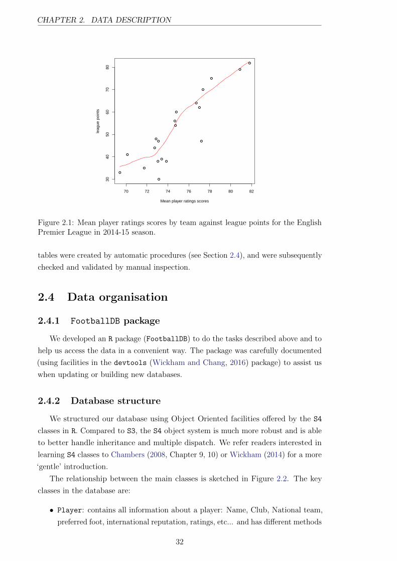
2.1 Mean player ratings scores by team against league points for the

English Premier League in 2014-15 season. . . . . . . . . . . . . . . . 32

2.2 Data structure: A black arrow from class A to class B means that

class A uses class B in its definition. A red arrow means that class A

inherits from class B. . . . . . . . . . . . . . . . . . . . . . . . . . . . 33

3.6 Frequency distributions of the number of children born to a woman

who has completed childbearing in Germany (n = 1, 243) . . . . . . . 45

3.1 Proportional errors in probabilities for the naıve computation and the

two Richardson corrections. Here α = 1, t = 1, β = 1.1. . . . . . . . . 52

3.2 Powers of stepsize h for error in probabilities for the naıve computation

and the two Richardson corrections. Here α = 1, t = 1, β = 1.2. . . . . 52



3.4 Powers of stepsize h for error in probabilities for the naıve computation

and the two Richardson corrections. Here α = 1, t = 1, β = 0.6. . . . . 53



4.1 Time to first goal as a competing risks with scoring intensities α1(t)

(home) and α2(t) (away). . . . . . . . . . . . . . . . . . . . . . . . . . 61

4.2 Scoring intensity for time to first goal by the home team (left) and

the away team (right). . . . . . . . . . . . . . . . . . . . . . . . . . . 63

4.3 Scoring process for the three first goals in a football match described

by a multi-state model. Each circle represents a state of the match

given by a scoreline. Arrows represent the possible transitions from

one state to another. When the score is x-y, x is always the home

team’s goals and y the away team’s goals. Thus a move ’upwards’ on

the diagram represents a home team goal and a move ’downwards’

represents an away team goal. . . . . . . . . . . . . . . . . . . . . . . 64

3

LIST OF FIGURES

4.4 Histograms of home goals (left) and away goals (right) with the

fitted Poisson and Weibull count models. The estimated parameters

(for the weibull models) are, for the home team, λH = 1.50 (0.04),

cH = 1.56 (0.03) and for the away team, λA = 1.10 (0.03) and cA =

0.85 (0.04), where the figures in parentheses are standard errors. . . . 66

4.5 Selecting the decay factor ξ by maximizing the objective function T (ξ)

defined in (4.4). The maximum occurs at ξ = 0.002 . . . . . . . . . . 70

4.6 Bookmaker implied probabilities (rescaled to sum to 1) versus model

probabilities for home win, draw and away win. . . . . . . . . . . . . 72

4.7 Bookmaker implied probabilities (rescaled to sum to 1) versus model

probabilities for over/under 2.5 goals. . . . . . . . . . . . . . . . . . . 72

5.1 Jamie Vardy’s overall score evolution between August 2012 and Jan-

uary 2016 (left) compared to his observed and expected rating between

August 2014 and January 2016 (right). . . . . . . . . . . . . . . . . . 81

5.2 Evolution of parameters as new data is added to the fitting sample. . 85

5.3 Calibration Curve for the simple model predicting outcomes in the

1X2 market. The size of the circles are proportional to the bin count. 87

5.4 Calibration Curve for the full model predicting outcomes in the 1X2

market. The size of the circles are proportional to the bin count. . . . 87

5.5 Influence of applying different thresholds on the betting performance

of the simple model with adjusted player ratings for the 1X2 market. 90

4

LIST OF TABLES

2.1 Ratings for Moussa Dembele playing in different positions. The table

shows he is best used as centre midfielder and maintains a high rating

for playing in any attacking position. . . . . . . . . . . . . . . . . . . 30

2.2 Descriptive Statistics for the player database for players registered to

play in the English Premier League in 2014-15 season. . . . . . . . . . 30

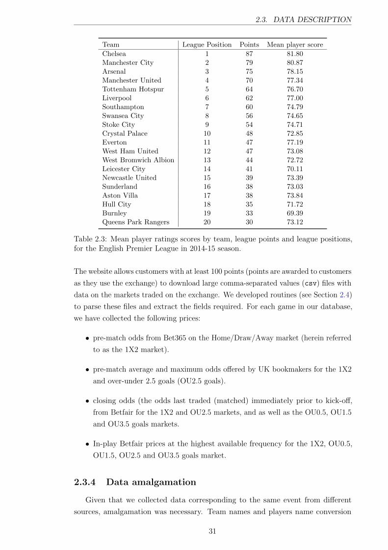
2.3 Mean player ratings scores by team, league points and league positions,

for the English Premier League in 2014-15 season. . . . . . . . . . . . 31

3.1 Number of children in the German fertility dataset. . . . . . . . . . . 45

3.2 Performance measure of the different computation methods available

for the Weibull count (German fertility data). The methods are

described in the main text. . . . . . . . . . . . . . . . . . . . . . . . . 46

3.3 Number of children (simulated data with artificially larger count) . . 47

3.4 Performance measure of the different computation methods available

for the Weibull count model (simulated data set) . . . . . . . . . . . 47

3.5 German fertility data: Model choice criteria for the various models. . 48

3.6 Regression model results for German fertility data . . . . . . . . . . 49

4.1 Goodness of fit summary for hazard of first goal for the home team

α1(t). Likelihood ratio test = 28.74 (p-value = 8.24 · 10−8, degrees of

freedom (df) = 1). . . . . . . . . . . . . . . . . . . . . . . . . . . . . 63

4.2 Goodness of fit summary for hazard of first goal for the away team

α2(t). Likelihood ratio test = 7.70 (p-value = 5.52 · 10−3, df = 1). . . 63

4.3 Goodness of fit summary for hazard of first three goals for the home

team. In all the previous likelihood ratio tests the degrees of freedom

are equal to one. . . . . . . . . . . . . . . . . . . . . . . . . . . . . . 65

4.4 Goodness of fit summary for hazard of first three goals for the away

team. In all the previous likelihood ratio tests the degrees of freedom

are equal to one. . . . . . . . . . . . . . . . . . . . . . . . . . . . . . 65

4.5 χ2 goodness-of-fit test statistics for the fitted Weibull count model

and Poisson distribution to home goals and away goals. . . . . . . . . 66

5

LIST OF TABLES

4.6 Estimated team strength parameters, based on the full five seasons

matches. Larger α’s indicate stronger attack, smaller β’s stronger

defence. . . . . . . . . . . . . . . . . . . . . . . . . . . . . . . . . . . 71

4.7 Comparison of the four models for football scores fitted (in-sample)

to the Premier League data. . . . . . . . . . . . . . . . . . . . . . . . 71

4.8 Summary of results when betting on the 1X2 market. . . . . . . . . . 73

4.9 Summary of results when betting on the over-under 2.5 goals market. 74

5.1 Results of ordinal regression fit to explain match outcome as a function

of the sum of each team’s player ratings. . . . . . . . . . . . . . . . . 78

5.2 Estimated parameters for the different specifications. Bootstrap stan-

dard errors based on 500 samples are presented in parentheses. . . . . 83

5.3 In-sample diagnostics for the four fitted models. . . . . . . . . . . . . 84

5.4 Scoring rules for the four models and bookmakers implied probabilities

applied to the 1X2 market. . . . . . . . . . . . . . . . . . . . . . . . . 88

5.5 Scoring rules for the four models and bookmakers implied probabilities

applied to the over-under 2.5 goals market. . . . . . . . . . . . . . . . 88

5.6 Betting strategy results for the 1X2 market. For each model the results

are shown for three values of the threshold: 0, 0.3 and 0.7. Also given

are the Sharpe ratios. . . . . . . . . . . . . . . . . . . . . . . . . . . . 90

5.7 Betting strategy results for the over-under 2.5 goals market. For each

model the results are shown for three values of the threshold: 0, 0.3

and 0.7. Also given are the Sharpe ratios. . . . . . . . . . . . . . . . 91

5.8 Expected league table using the simple model with adjusted player

ratings generated using 1000 simulations using the current English

Premier League teams, and adding Paris Saint Germain (France) and

Celtic (Scotland). Expected points computed using the theoretical

formulae are given in parenthesis. . . . . . . . . . . . . . . . . . . . . 92

5.9 Probability (%) of winning the English Premier League, finishing in

the top 3, 4 or 5, or finishing in the bottom 4. Results are based

on using the simple model with adjusted player ratings to simulate

the league 1000 times. Two additional teams have been added to the

league: Paris Saint Germain (France) and Celtic (Scotland). . . . . . 93







6

ABSTRACT

7

ABSTRACT

The University of Manchester

Tarak Kharrat

Doctor of Philosophy

A Journey Across Football Modelling with Application to Algorithmic

Trading

February 27, 2016

In this thesis we study the problem of forecasting the final score of a football

match before the game kicks off (pre-match) and show how the derived models can

be used to make profit in an algorithmic trading (betting) strategy.

The thesis consists of two main parts. The first part discusses the database and

a new class of counting processes. The second part describes the football forecasting

models.

The data part discusses the details of the design, specification and data collection

of a comprehensive database containing extensive information on match results

and events, players’ skills and attributes and betting market prices. The database

was created using state of the art web-scraping, text-processing and data-miming

techniques. At the time of writing, we have collected data on all games played in

the five major European leagues since the 2009-2010 season and on more than 7000

players.

The statistical modelling part discusses forecasting models based on a new

generation of counting process with flexible inter-arrival time distributions. Several

different methods for fast computation of the associated probabilities are derived and

compared. The proposed algorithms are implemented in a contributed R package

Countr available from the Comprehensive R Archive Network.

One of these flexible count distributions, the Weibull count distribution, was used

to derive our first forecasting model. Its predictive ability is compared to the models

previously suggested in the literature and tested in an algorithmic trading (betting)

strategy. The model developed has been shown to perform rather well compared to

its competitors.

Our second forecasting model uses the same statistical distribution but models

the attack and defence strengths of each team at the players level rather than at

a team level, as is systematically done in the literature. For this model we make

heavy use of the data on the players’ attributes discussed in the data part of the

thesis. Not only does this model turn out to have a higher predictive power but it

also allows us to answer important questions about the ‘nature of the game’ such as

the contribution of the full-backs to the attacking efforts or where would a new team

finish in the Premier League.

8

DECLARATION

I declare that no portion of this work referred to in this thesis has been submitted

in support of an application for another degree or qualification of this or any other

university or other institute of learning.

9

COPYRIGHT

(i) The author of this thesis (including any appendices and/or schedules to this

thesis) owns certain copyright or related rights in it (the ”Copyright”) and s/he

has given The University of Manchester certain rights to use such Copyright,

including for administrative purposes.

(ii) Copies of this thesis, either in full or in extracts and whether in hard or

electronic copy, may be made only in accordance with the Copyright, Designs

and Patents Act 1988 (as amended) and regulations issued under it or, where

appropriate, in accordance with licensing agreements which the University has

from time to time. This page must form part of any such copies made.

(iii) The ownership of certain Copyright, patents, designs, trade marks and other

intellectual property (the ”Intellectual Property”) and any reproductions of

copyright works in the thesis, for example graphs and tables (”Reproductions”),

which may be described in this thesis, may not be owned by the author and may

be owned by third parties. Such Intellectual Property and Reproductions cannot

and must not be made available for use without the prior written permission

of the owner(s) of the relevant Intellectual Property and/or Reproductions.

(iv) Further information on the conditions under which disclosure, publication

and commercialisation of this thesis, the Copyright and any Intellectual

Property University IP Policy (see http://documents.manchester.ac.uk/

display.aspx?DocID=24420 ), in any relevant Thesis restriction declarations

deposited in the University Library, The University LibraryaAZs regulations

(see http://www.library.manchester.ac.uk/about/regulations/ ) and in

The University’s policy on Presentation of Theses.

11

http://documents.manchester.ac.uk/display.aspx?DocID=24420

http://documents.manchester.ac.uk/display.aspx?DocID=24420

http://www.library.manchester.ac.uk/about/regulations/

ACKNOWLEDGEMENTS

I would like to thank Dr. Georgi Boshnakov for being a constant source of

motivation and encouragement. I would also like to thank Professor Ian McHale

for his constant help and support, for constructive discussions and for being so

enthusiastic and receptive to my new ideas. Thanks to Professor Rose Baker for

collaboration and useful advise. Last but not least, my gratitude to Professor

Matthias Heil for introducing me to the University of Manchester and its brilliant

School of Mathematics.

13

CHAPTER

ONE

INTRODUCTION

“ Gambling is risk-taking. It might be said the owner of a casino

gambles, takes risks, but he has the odds in his favour, so that’s

intelligent gambling. If I wanted to gamble, I’d buy the casino.

”Jean Paul Getty, Sr, 1982

Although it is difficult to determine the exact date and origin of gambling on the

outcome of sporting events, we do know that sports and betting have co-existed for

thousands of years. It is well-known that in ancient Rome it was legal to bet at the

circus or in chariot races and that even the Roman emperors of the time indulged in

gambling. In more recent times, in the United Kingdom (UK) for example, there

has been a long tradition of sports betting where people have bet on the outcome of

horse races, cockfights and bare-knuckle brawls from as early as the 1700’s. Indeed,

the rules of cricket were first formalised in 1728 as a result of gamblers wanting more

transparency and fairness.

Sports betting now plays a large part of modern society across many cultures

and is truly a global activity. Betting shops were legalised in the UK by the Betting

and Gaming Act 1960 (UK Parliament, 1960) and since then, a gradual relaxation

of the restrictions on gambling has allowed for innovation and the introduction

of new products as bookmakers fine tune their offerings to suit customers’ tastes

and demands. Following decades of evolution, and especially since the onset of the

internet and the in-play market, the sports betting industry is now large. In 2012,

Darren Small, Director of Integrity at betting and sports data analysts Sportradar

said “The current estimations, which include both the illegal markets and the legal

markets, suggest the sports match-betting industry is worth anywhere between $700bn

and $1tn (£435bn to £625bn) a year”1. It is believed that, excluding horse racing2,

1In the UK, the global sports sector was estimated to be worth around $130bn in 2012 withforecasts that it will reach over $146bn in 2014

2In the UK, horse race betting dominates with 51% of the market. The second largest is football

15

CHAPTER 1. INTRODUCTION

70-85% of the bets placed are on the world’s most popular sport, football.

These estimates of the size of the sports betting industry (in the UK) make it

comparable in value to that of manufacturing ($155bn in 2014).

In order to attract and keep costumers, licensed bookmakers offer upwards of

200 different markets on football matches around the globe. Punters can bet on the

first and last goalscorer, the correct score, the half-time score, the number of goals,

and many, many more. These markets can be crudely categorised into two types:

pre-match and in-play markets. Before the dawn of the internet, the majority of

markets (and bets) were placed before the start of a game and bets were settled after

the final whistle. This type of betting is known as pre-match betting, or fixed-odds

betting1. Generally speaking, the bookmakers hope to produce a profit by offering

lower odds than those they believe to be fair and hence accurately computing the

‘fair’ or ‘true’ prices (i.e the inverse of the probabilities) is of crucial importance for

both the bookmakers and the punters.

As explained by Dixon and Pope (2004), not that long ago (as recently as 2008),

setting odds for the pre-match market was mainly subjective: a panel of experts with

extended experience in setting odds, met to discuss the upcoming matches and used

their judgement and knowledge of the current state of each team to ‘come up’ with

numbers for the home win, draw and away win prices. Given the extended number

of markets proposed nowadays, the huge amount of data available (historical results,

players information, . . . ) and the development of statistical models to forecast match

outcomes, we do not believe this approach is practicable. Private correspondence

with representatives from major UK bookmakers confirms that the offered odds are

in fact generated by statistical models, although adjusted by ‘traders’ to match the

‘market’ belief and incorporate available information not processed by the model

being used. Therefore, developing a ‘pre-match’ model to predict the outcome of

football matches remains a question of interest and the concern of the second part of

this work.

The growth of the internet and mobile devices with quick access to odds has

made betting generally much more accessible. Satellite television channels and

increased coverage of live football matches around the world has increased interest

and opportunity for both the punter and the bookmaker. The growth of the internet

also instigated the appearance of betting exchanges2, which serve as peer-to-peer

betting platforms, where individuals are allowed to bet directly with each other, and

not with a bookmaker. In most cases the exchange takes no risk on the outcome of

with 15% of the market.1 fixed-odds is the name typically used in the industry. Its origin is related to the fact that odds

used to be fixed by the bookmakers several days before the match, and were not adjusted as betswere placed even if new information was received. Although true in the recent past, this is not thecase anymore as reported in Constantinou and Fenton (2012a). Therefore, in this work pre-matchis preferred.

2Betfair, currently the largest exchange in Europe, is estimated to gather almost 10% of thesize of the football betting market in the UK.

16

1.1. CONTRIBUTION

the events, as they take a commission from the customers. Rather, the punters on

either side of the bet take the risk as one backs an outcome whilst another must ‘lay’

it 1.

The emergence of exchanges has undoubtedly brought several innovations to the

industry. First, in order to remain competitive with the exchanges, the increase of

competition forced bookmakers to reduce their over-round2 from between 10% to 15%

in the beginning of the century to around 5% on average now. Besides, exchanges also

offer the opportunity to place orders algorithmically via their application program

interface (API). The immediate consequence is that a 100% automated strategy

based on statistical models can be implemented, back-tested and executed. In the

second part of this thesis, some examples of (profitable) fully automated betting

strategies are studied.

1.1 Contribution

A new generation of pre-match models for estimating probabilities of the final

score grid is developed in the second part of this thesis. The novelty comes first from

adopting a more flexible counting process which itself is derived by a relaxation of

the usual Poisson assumption made almost systematically in the literature. A new

family of counting processes based on flexible inter-arrival time distributions (not

necessary exponential with constant hazard rate) is introduced in the first part of this

thesis. Several algorithms for fast computation of the count probabilities are derived,

compared and implemented in an R (R Core Team, 2015) package which we have

called Countr. The package is available on the Comprehensive R Archive Network

(CRAN 3) and a paper for the Journal of Statistical Software is in preparation. One of

these flexible distributions is used by our first model suggested in part 2 (Chapter 4).

This model requires the same type of data as the ones usually used in the academic

literature 4 meaning that the model can easily be compared to other models. Its

performance is tested in a betting strategy that could be classified in the ‘statistical

arbitrage’ type.

The second novelty comes from the data we collected and used in the second model

suggested in part 2 (Chapter 5). A large (“big data”) database containing (i) match

details including the final score and the timings of goals and red and yellow cards

(event data); (ii) player skills and attributes including ratings for players on a match

by match basis (player data); and (iii) bookmakers and exchange prices (market data)

was collected. A second R package FootballDB was created for extracting (scraping),

cleaning and organising these data.

1back the complementary event, i.e, bet on the event not happening.2Also known as commission and is defined as the difference between a bookmaker’s odds and

the fair odds, often expressed as a percent.3https://cran.r-project.org/4historical match scores.

17

https://cran.r-project.org/

CHAPTER 1. INTRODUCTION

Our first model, and all the previous models suggested in the literature, is a team

based model in that the only information that is fed into it is the identity of the team

(and its past results). Here however, we propose using a player-based model whereby

the information fed into the model includes the identity and ratings of the players on

the pitch for each team. The forecasting accuracy of this model is compared to the

bookmakers predictions and also tested in the same automated betting strategy as we

test our team-based model. In addition to providing promising results when used for

betting, we propose some novel uses of our player-based model, including answering

interesting questions about the ‘nature of the game’ such as the contribution of the

full-backs to the attacking efforts, or where would a new team finish in the Premier

League.

1.2 Thesis outline

This thesis is organised into two halves: the first half is titled Preparing the

Ground and presents the preliminary work needed to produce the main results

discussed in the second part: Forecasting Models and Algorithmic Trading. Chapter 2

describes the data. It explains how the database was created, cleaned and organised.

Chapter 3 discusses the derivation of a new family of count processes based on renewal

processes with flexible inter-arrival time distributions. The results of Chapter 3 will

be used to derive our first forecasting model described in Chapter 4. Its output will be

used in an algorithmic trading strategy on the Home/Draw/Away and Over/Under

2.5 goals markets. A second model using this flexible count process together with

player-level information is described in Chapter 5. The same betting strategy was

implemented and in depth analysis of its returns studied. Conclusions and future

work are collected in Chapter 5.6.

1.3 Publications

The work presented in this thesis resulted in the following papers:

• Chapter 3:

– Baker and Kharrat (2016): under review at the journal of Computational

Statistics & Data Analysis.

– Baker et al. (2016): in preparation for submission to the Journal of

Statistical Software

• Chapter 4: Boshnakov et al. (2016a): submitted to the International Journal

of Forecasting. The paper has been reviewed and is currently under revision.

• Chapter 5: Boshnakov et al. (2016b): in preparation.

18

1.4. CONTRIBUTED SOFTWARE

• Boshnakov and Kharrat (2016): submitted to the Journal of Statistical Software

in February 2014. The paper has been reviewed and is currently under revision

(but not discussed in this thesis).

1.4 Contributed software

In this work, special care was taken to produce (trustworthy) software and code

that are computationally efficient and can deal with numerical issues that typically

arise when dealing with (big) data. Therefore, some sections contain (and discuss)

chunks of code. The software produced was mainly written in R following (strictly)

the coding style guide collected in Appendix 1. However, most of the heavy linear

algebra computation was executed in C++ using routines from Rcpp (Eddelbuettel and

Francois, 2011) and RcppArmadillo (Eddelbuettel and Sanderson, 2014) libraries.

The list of contributed packages can be found below:

• StableEstim: published on CRAN in January 2014.

• Countr: published on CRAN in February 2016.

• FootballDB: a beta version exists but an improved (more stable) version is in

preparation.

19

Part I

Preparing the Ground

21

In this first part, we describe the preliminary work needed to derive the forecasting

models of part 2.

The first Chapter is dedicated to the data. We describe the data collection

procedure, the cleaning steps, how we organise it and software developped to do so.

A brief description of the different information collected is also presented.

The second Chapter is the result of a collaboration with Prefessor Rose Baker

(University of Salford). We present several methods to compute the probability of

flexible event count distributions derived from renewal processes. The performance of

the different methods is compared and a contributed R (R Core Team, 2015) package

Countr was developped. This research was also turned into a paper submitted to

the journal of Computational Statistics & Data Analysis in February 2016.

23

CHAPTER

TWO

DATA DESCRIPTION

“ In God we trust; all others must bring data.

”William Edwards Deming,

2.1 Introduction

The increasing interest in association football, together with the development

of new broadcasting technologies over the past two decades have resulted in an

unprecedented change in the way we watch and engage with football matches. Not

that long ago, the only data that were available were the final result (number of

goals scored by each team) and information such as the time of goals or the identity

of the players on the pitch was almost impossible to access in a format usable by

a statistician (a well-structured, large sample and trustworthy data set). In fact,

among the huge amount of literature published on forecasting football games, only a

few examples (Dixon and Robinson (1998), Volf (2009), Titman et al. (2015)) used

information on the time of goals and cards shown for example. Although several

providers (Opta and Prozone, for example) offer access to detailed match event

descriptions, the costs of such data remain a barrier for most of the academic world.

At the same time, the rapid growth of the internet has drastically changed the

way we share, collect, and publish data. It is certainly possible nowadays to find a

website that contains the level of details (on football matches) we are looking for.

What was once a fundamental problem for sports statisticians - the scarcity, cost

and inaccessibility of detailed data - is quickly turning into an abundance of data.

This turn of events should encourage statisticians, at least in the academic world, to

consider the internet as a new fabulous source of data.

A consequence of the internet now being a valuable source of data is that

traditional techniques for collecting data may no longer suffice. For example, to

25

CHAPTER 2. DATA DESCRIPTION

overcome the tangled masses of data available the new generation of statisticians

need to develop skills such as a deep understanding of modern data transfer protocols

and web scraping techniques. Therefore, a non-negligible amount of our research

time in this project was devoted to the development of those skills and the database

described in this chapter is the result of this effort.

We have developed some semi-automated procedures to build up a large football

database using state of the art web-scraping, text processing and data-mining

techniques. These procedures were tasked with collecting data from several websites

as described later in this chapter. While we cannot hope to have a fully automated

robust program, we reached a high level of autonomy and the user has almost nothing

to do apart of checking that nothing went wrong. Nevertheless, our procedure is

highly dependent on the website structure and any change in this structure will

inevitably affect our routines. The web-scraping procedure together with the user

input required is described in Section 2.2.

The database we have built has information on three different aspects of the

game:

1. Results data including team lineups for each match, timings of goals, red and

yellow cards for every game in the last seven years in the five major European

leagues: England Premier League, France Ligue 1, Italy Serie-A, Spain Liga

Primera and Germany Bundesliga 1.

2. Player ratings collected on a weekly basis from video game websites. These

player ratings are created and maintained by networks of expert scouts working

for the two world leading video games firms: EA SPORTS who produce a

yearly version of FIFA and their competitor KONAMI with their celebrated

Pro Evolution Soccer. The use of data collected by video games is a recent

development in the football industry1 and sports media2 which suggests that

the data has some predictive value (which will be demonstrated in the second

part of this thesis). More information on the players’ database can be found

in Section 2.3.2. In addition to these player ratings, we also obtained the EA

SPORTS Player Performance Indicator (PPI) ratings3. The PPI gives players

ratings for their performances in each match in which they play.

3. Betting market data for both pre-match odds from various UK bookmakers as

well as the pre-match and in-play prices from the Betfair exchange are available

for every game. This data will be used in the second part of this thesis to test

our various forecasting models in an automated trading strategy. For details

about the market data, we refer the reader to Section 2.3.3.

1http://www.theguardian.com/technology/2014/aug/12/2http://www.telegraph.co.uk/sport/football/babb/11780655/

Sky-Sports-use-Football-Manager-database-to-profile-players-in-real-life.html3These data were provided to us in a ready to use format and needed no scraping or cleaning.

26

http://www.theguardian.com/technology/2014/aug/12/

http://www.telegraph.co.uk/sport/football/babb/11780655/Sky-Sports-use-Football-Manager-database-to-profile-players-in-real-life.html

http://www.telegraph.co.uk/sport/football/babb/11780655/Sky-Sports-use-Football-Manager-database-to-profile-players-in-real-life.html

2.2. BUILDING A FOOTBALL DATABASE

Naturally, such a big database needs to be organised and structured to enable

quick and easy access to the various levels of detail required. A collection of R (R

Core Team, 2015) S4 classes and methods has been developed for this purpose and

gathered in a package which we have called FootballDB. The use of FootballDB

facilitates data preparation for model fitting and general data exploration tasks. At

the heart of the package are methods for some given classes to get a limited number

of tasks completed. This procedure is explained in Section 2.4.

2.2 Building a football database

Loosely speaking, web-scraping means building software to extract data from

a website. It involves (i) loading the website source code, (ii) parsing its content

and then (iii) storing the required information. It assumes that the website has a

stable structure and does not change over time, and that the information needed is

accessible from the page source code.1

All the procedures described in this Chapter were implemented in R. This choice

can be justified by two main reasons: first, the contributed packages from the

Comprehensive R Archive Network (CRAN) offers all the necessary building blocks

to achieve this task, and second, and most importantly, we wanted to use a single

piece of software for all steps in the project: data collection, data analysis and model

fitting.

2.2.1 Loading the website source code

The RCurl package (Lang, 2007) was used to compose http requests. The package

is actually a wrapper to the C library libcurl2 and uses it behind the scene to

perform the request and retrieve the response. The main function used is getURL().

It requires the url address and it is preferred to specify the type of encoding used by

the website to avoid any issue that may happen when converting special characters

(mainly accents - which, in this project, are frequently used in player names). The

call to getURL() returns a character string that contains the page source code.

In order to build a database, one has to to retrieve the information related to

each match (or player). The first problem that we had to solve was to identify the

web-page url related to each match. Usually, the web-pages have a common name

and a unique identifier number for each match (or player). However, some manual

input was needed to identify the sequence of relevant identifiers for our purpose. A

second issue may arise when the website does not allow a large number of consecutive

requests. In fact, most of the websites containing relevant data are able to identify

1Some websites load their content by a call to a javascript which makes the source codeunavailable and hence prohibits scraping.

2libcurl needs to be installed on your machine in order to use the package

27


automatic requests and will ban the responsible IP address from sending any further

requests. Depending on the website, we had to stop our program for some time (5

minutes) after a relative small number of requests sent (usually 10) and start again.

Therefore, the extraction took a long time (up to several weeks for some websites).

2.2.2 Parsing the web-page content

Once extracted, the content of the web-page had to be ‘parsed’. When the page

was written in a standard fashion such as html/xml language or JSON, the task is

slightly simplified by the use of contributed packages such as XML (Lang, 2015)) or

jsonlite (Ooms, 2014) to the R environment. One just has to identify the ‘road’

to the desired node/object and use the package facilities to extract it. The task

becomes more challenging when the web-page does not follow standard practice

or has an incomplete html/xml structure. In this case, we turn to text-processing

techniques such as regular expression searching using routines from the package

stringr (Wickham, 2015). This approach is inevitably more prone to errors and

requires more manual checking for validation.

2.2.3 Cleaning

Cleaning is a necessary task if one is willing to build a trustworthy database.

Some automatic procedures were designed (to check that all fixtures were downloaded

successfully) but ultimately manual checking was unavoidable. We will not detail

the different cleaning steps as it adds little to this description but it is worthy of

mention since it took many days to make sure that the data are trustworthy and can

be relied upon.

2.3 Data description

2.3.1 Match data

Match data were obtained from http://www.football-lineups.com/. We col-

lected timing of goals (minutes), type of goals (when available), identity of the scorer

(and the player delivering the assist when available), starting lineups (players names),

time of substitution and identity of the associated players and yellow and red cards

given (timing and identity of the associated players).

The scraping was entirely made by text-processing as the website didn’t respect

a complete html/XML syntax. The immediate consequence is that a long time was

needed to introduce missing inputs when the algorithm failed to extract them (due

to missing fields in the loaded source code). A large number of checking procedures

were used to make sure the extracted data were trustworthy (no repetition in player

28

http://www.football-lineups.com/

2.3. DATA DESCRIPTION

names, subbed players were part of the starting lineups, scorers are playing at the

time of scoring ...).

2.3.2 Player data

We collected player ability ratings from two sources: the EA SPORTS FIFA

and KONAMI PRO EVOLUTION SOCCER computer games. The data are

available from http://sofifa.com/ and http://pesdb.net. The data are produced

and maintained by a global network of more than 1000 scouts, who watch games

and score players on more than 40 criteria describing players abilities in different

skill areas of the game. For example, players are given scores out of 100 for tackling,

passing, shooting, speed, aggression, and so on. A detailed description of the players

main attributes can be found in Appendix 2.

In addition to providing ratings for each skill area, players are assigned an ‘overall

rating’. This overall rating is calculated from the individual skill area ratings and

summarises the effectiveness of the player when playing in his natural (preferred)

positions (see Appendix 2 for a list of the position considered). This rating is hence

position dependent and may change dramatically if a player is used in a position he

is not comfortable playing in. Consider the example of a centre midfielder with a

score of 80 (out of 100). If that player was asked to play as a centre back, then his

score of 80 would be inappropriate, as he would not be as effective playing in an

unfamiliar position to which he is not accustomed, and to which his particular skill

set is not suitable. Fortunately, the databases also give scores for players playing in

other positions. An example with Moussa Dembele (Tottenham Hotspur) is given in

Table 2.1

At the time of writing, we have collected data on more than 7000 players. The

maximum score of any player in the database was attributed to Lionel Messi of

Barcelona (94) with Cristiano Ronaldo of Real Madrid in second place scoring

93. For players registered to play in the English Premier League in the 2015-16

season, the mean strength was 75.7. The number of players, the mean score and

standard deviation in scores for each playing position is given in Table 2.2. Perhaps

unsurprisingly, the position with the maximum mean strength is striker, closely

followed by central midfielder. The weakest position in the Premier League is that of

full-back, and the position with the highest variation in ability is the goalkeeper.

Table 2.3 and Figure 2.1 show the mean score of each team (for the actual line-

ups that played in matches) and the team’s league position for the 2014-15 season.

Spearman’s rank correlation between the mean lineup strength and the league final

points is 0.83 demonstrating a strong relationship between the individual player

scores and the results of the team. This provides some evidence that the player

scores have information in them. The player scores will be used in the second part of

this thesis in a pre-match forecasting model.

29

http://sofifa.com/

http://pesdb.net


Table 2.1: Ratings for Moussa Dembele playing in different positions. The tableshows he is best used as centre midfielder and maintains a high rating for playing inany attacking position.

Position Rating

LW, RW 78ST 76

LF, CF, RF 78CAM 79

LM 78CM 79RM 78

CDM 77LWB 75

LB 74CB 74RB 73

RWB 74SW 72GK 15

Position N Minimum Maximum Mean Median Standard deviation

Goalkeeper 45 61 85 74.56 75 6.20Central defender 85 54 86 74.08 75 5.64Full-back 81 57 82 71.59 72 5.38Central midfielder 132 56 87 75.08 75 5.70Wide midfielder/winger 92 60 88 74.95 75 5.21Striker/forward 77 59 89 75.10 75 5.97

Table 2.2: Descriptive Statistics for the player database for players registered to playin the English Premier League in 2014-15 season.

In addition to the video game data, we were also provided with data from the

EA SPORTS Player Performance Index (PPI). The PPI is the official player ratings

system of the English Premier League and is described in McHale et al. (2012b). To

summarise, it awards players for their actions on the pitch. The relative award for

the actions is such that actions associated with a team having a higher number of

shots are awarded more highly than other actions. For example, a player performing

a cross receives more points than a player performing a pass in his own half of the

pitch. The data did not need scraping and were provided in a clean format. We

discuss the need for both the video game data, and the match-by-match performance

ratings in Chapter 5

2.3.3 Market data

Pre-match odds were simply downloaded from http://www.football-data.co.

uk/. The Betfair exchange prices were obtained from http://data.betfair.com/.

30

http://www.football-data.co.uk/

http://www.football-data.co.uk/

http://data.betfair.com/

2.3. DATA DESCRIPTION

Team League Position Points Mean player score

Chelsea 1 87 81.80Manchester City 2 79 80.87Arsenal 3 75 78.15Manchester United 4 70 77.34Tottenham Hotspur 5 64 76.70Liverpool 6 62 77.00Southampton 7 60 74.79Swansea City 8 56 74.65Stoke City 9 54 74.71Crystal Palace 10 48 72.85Everton 11 47 77.19West Ham United 12 47 73.08West Bromwich Albion 13 44 72.72Leicester City 14 41 70.11Newcastle United 15 39 73.39Sunderland 16 38 73.03Aston Villa 17 38 73.84Hull City 18 35 71.72Burnley 19 33 69.39Queens Park Rangers 20 30 73.12

Table 2.3: Mean player ratings scores by team, league points and league positions,for the English Premier League in 2014-15 season.

The website allows customers with at least 100 points (points are awarded to customers

as they use the exchange) to download large comma-separated values (csv) files with

data on the markets traded on the exchange. We developed routines (see Section 2.4)

to parse these files and extract the fields required. For each game in our database,

we have collected the following prices:

• pre-match odds from Bet365 on the Home/Draw/Away market (herein referred

to as the 1X2 market).

• pre-match average and maximum odds offered by UK bookmakers for the 1X2

and over-under 2.5 goals (OU2.5 goals).

• closing odds (the odds last traded (matched) immediately prior to kick-off,

from Betfair for the 1X2 and OU2.5 markets, and as well as the OU0.5, OU1.5

and OU3.5 goals markets.

• In-play Betfair prices at the highest available frequency for the 1X2, OU0.5,

OU1.5, OU2.5 and OU3.5 goals market.

2.3.4 Data amalgamation

Given that we collected data corresponding to the same event from different

sources, amalgamation was necessary. Team names and players name conversion

31


●

●

●

●

●

●

●

●

●

●●●

●

●

●● ●

●

●

●

70 72 74 76 78 80 82

3040

5060

7080

Mean player ratings scores

leag

ue p

oint

s

Figure 2.1: Mean player ratings scores by team against league points for the EnglishPremier League in 2014-15 season.

tables were created by automatic procedures (see Section 2.4), and were subsequently

checked and validated by manual inspection.

2.4 Data organisation

2.4.1 FootballDB package

We developed an R package (FootballDB) to do the tasks described above and to

help us access the data in a convenient way. The package was carefully documented

(using facilities in the devtools (Wickham and Chang, 2016) package) to assist us

when updating or building new databases.

2.4.2 Database structure

We structured our database using Object Oriented facilities offered by the S4

classes in R. Compared to S3, the S4 object system is much more robust and is able

to better handle inheritance and multiple dispatch. We refer readers interested in

learning S4 classes to Chambers (2008, Chapter 9, 10) or Wickham (2014) for a more

‘gentle’ introduction.

The relationship between the main classes is sketched in Figure 2.2. The key

classes in the database are:

• Player: contains all information about a player: Name, Club, National team,

preferred foot, international reputation, ratings, etc... and has different methods

32

2.4. DATA ORGANISATION

to plot(), extract() and print() summaries of these attributes.

• LineUp: information about a team lineup for a given match: players on the

pitch, and any substitutions used.

• Match: collects all information related to a given match. This class has a

method ModelData() to assist user creating data sets to fit specific models.

Competition

Match

Events

Team Goals Shots Cards

LineUp ShotsOnTarget ShotsOffTarget RedCard YellowCard

Player

Skills TeamGeneralInfo

Attacking Defending Playing Movement Power Mentality Club

Figure 2.2: Data structure: A black arrow from class A to class B means that class Auses class B in its definition. A red arrow means that class A inherits from class B.

2.4.3 Database update

The database is updated automatically via a scheduled task running on Monday

of every week at midnight) using procedures from FootballDB. It takes around 4

hours to update the players database and around 35 minutes to extract match event

data. The market data from the Betair exchange needs to be downloaded manually

but once obtained, they get processed almost instantaneously.

33


2.5 Conclusion and future work

Building up the database was a long term project started at an early stage of the

PhD project. It took us around 18 months to build the FootballDB package, run

the extractions and validate the resulting data. The database is stored in a collection

of RDS objects that are updated every week. The size of the resulting database is

around 4Gb.

Future work will include the extraction of data related to new leagues. Data can

be collected for the Netherlands, Brazil, Russia and the USA for example. Further,

even broader, richer data can be collected with information on player suspensions

and injuries.

34

CHAPTER

THREE

EVENT COUNT DISTRIBUTIONS FROM RENEWAL

PROCESSES: FAST COMPUTATION OF

PROBABILITIES

abstract

Discrete distributions derived from renewal processes, i.e. distributions of the

number of events by some time t are beginning to be used in econometrics and health

sciences. A new fast method is presented for computation of the probabilities for

these distributions. We calculate the count probabilities by repeatedly convolving

the discretized distribution, and then correct them using Richardson extrapolation.

When just one probability is required, a second algorithm is described, an adaptation

of De Pril’s method, in which the computation time does not depend on the ordinality,

so that even high-order probabilities can be rapidly found. Any survival distribution

can be used to model the inter-arrival times, which gives a rich class of models with

great flexibility for modelling both underdispersed and overdispersed data. This work

could pave the way for the routine use of these distributions as an additional tool

for modelling event count data. An empirical example using fertility data illustrates

the use of the method and was fully implemented using an R (R Core Team, 2015)

package Countr (Baker et al., 2016) developed by the authors and available from the

Comprehensive R Archive Network (CRAN).

3.1 Introduction

Modelling a count variable (the number of events occurring in a given time

interval) is a common task in econometrics. The standard approach is to use the

Poisson model, where Y |x ∼ Poisson(E(Y |x) = exp(x′γ)). Here Y is predicted given

covariates with values x, using regression coefficients γ. This model was built around

a one to one correspondence between the count model (Poisson) and the distribution

of the inter-arrival time (exponential). Perhaps this conceptual elegance contributed

35

CHAPTER 3. EVENT COUNT DISTRIBUTIONS FROM RENEWALPROCESSES: FAST COMPUTATION OF PROBABILITIES

to its popularity. With this elegance comes some limitation: the Poisson model

restricts the (conditional) variance to be equal to the (conditional) mean. This

situation is rarely observed in real life data and among the thousands of alternatives

proposed in the literature (see for example Winkelmann (2013) or Cameron and

Trivedi (2013) for a review), only a few retain the correspondence between the count

model and the timing process.

This correspondence is not only a conceptual elegance but also offers the researcher

the flexibility to model the aspect (counting or timing) that he/she knows better

(from the available data) and to draw conclusions (typically prediction) using the

other. A very good example in the marketing context was given in McShane et al.

(2008).

Another limitation of the Poisson model results from the memorylessness property

of the exponential distribution. In fact, this property states that the probability of

having an arrival during the next [t, t+ ∆t] time period (where t > 0 and ∆t > 0) is

independent of when the last arrival occured. In many situations, this assumption

is not realistic and the history of the process can be informative about future

occurrences. For example, someone who consulted the doctor many times recently is

more likely to have a higher number of doctor visits in the future (they are probably

ill) than someone who did not. This is usually dealt with using the negative binomial

model, where overdispersion is accommodated by making the hazard of a series of

visits of an individual a random variable from a gamma distribution.

The distribution of N(t), the number of renewal events by some time t offers an

alternative to the Poisson model that preserves the connection between the count

model and the timing process, but allows a more general event count distribution.

Inter-arrival times between events are still assumed to be independent and identically

distributed but the constant hazard function arising from an exponential distribution

is replaced by a nonconstant hazard function. These type of models display duration

dependence where negative duration dependence is obtained by a decreasing hazard

function (of time) and positive duration dependence by an increasing hazard function.

This gives a more flexible count distribution, and in particular, allows it to be

overdispersed or underdispersed.

It is possible to generalise further to a modified renewal process, which allows the

time to the first event to have a different distribution from later event inter-arrival

times. This gives rise to a type of hurdle model (see e.g. Mullahy (1986) for an

account of hurdle models). If for example we kept the same survival distribution, but

reduced the hazard function, we would have a distribution with an excess of zero

events, where the initial hazard function could be a different function of covariates

from later ones. Conversely, if the initial hazard function is higher, then we would

see few zero events. Thus this class of distributions is flexible enough to analyse data

with an abnormal number of zero events, and often will have some foundation in

36

3.2. POSSIBLE COMPUTATION METHODS FOR RENEWAL PROCESSES

reality.

In the simplest hurdle model, we have a Bernoulli trial, followed by a zero-

truncated Poisson distribution for the number of events. Greene (2011, chapter 25)

comments apropos of hurdle models that it is difficult to test whether the hurdle

is really there or not (‘regime splitting’ is occurring), as the hurdle model cannot

reduce to the Poisson model and so give a nested model. However, modelling with a

modified renewal process, we have to test only that the scale of the hazard function

for the first event is equal to that for the later events, when the hurdle model reduces

to a regular model. This can be done with a chi-squared test derived from the

log-likelihood function. Also, tests for under or overdispersion are difficult with

hurdle models, where the excess of zeros anyway induces overdispersion. With the

modified Weibull process, a test for under or overdispersion even given a hurdle can

be carried out by using a chi-squared test based on the log-likelihood to test whether

the shape parameter β departs from unity. Renewal processes thus give rise to a

rich and tractable class of models, but the slowness or unavailability of methods of

computing the probabilities has so far largely prohibited their use.

Winkelmann (1995) was the first to comment on the usefulness of renewal process

models and derived a count model based on gamma distributed inter-arrival times.

The choice of the gamma distribution was justified by computational necessity. In

fact, the reproductive property of the gamma distribution, i.e. sums of independent

gamma distributions are gamma distributed, leads to a simple form for the derived

gamma count probability.

The remainder of this chapter is laid out as follows. We start by reviewing the

possible computation methods in Section 3.2. Section 3.3 discusses the situation

when all probabilities up to the mth are required. An alternative method is described

in Section 3.4 when only the mth probability is of interest, in which case a faster

computation can be done. Improvement by Richardson extrapolation is developed in

Section 3.5. Section 3.6 contains a discussion on the generalisations to other survival

distributions. In Section 3.7, we re-analyse the same data used in Winkelmann (1995)

and compare a sequence of nested models starting with the basic Poisson regression.

Using this approach allows us to highlight which features of the model are most

critical to describe the data at hand. Future work and concluding remarks can be

found in Section 3.8.

3.2 Possible computation methods for renewal pro-

cesses

In this section, we review the possible methods for computing the count prob-

abilities for other survival distributions besides the gamma. Lomnicki (1966) gave

a method for computing a count model with Weibull interarrival times, based on

37


an expansion of the exponential function into powers of t and also into Poissonian

functions. McShane et al. (2008) used the expansion into powers of t to evaluate the

discrete distribution probabilities and fit an underdispersed dataset (the one used in

Winkelmann (1995) and fitted here). The same approach has been used in Jose and

Abraham (2011) and Jose and Abraham (2013) to derived a counting process with

Mittag-Leffler and Gumbel inter-arrival times respectively.

An expansion of the negative exponential is slow to converge. We found that this

method can be improved by using techniques such as the Euler and van-Wijngaarden

transformations (Press et al., 2007, Chapter 5), which are designed to speed up

convergence of alternating-sign series. Nevertheless, the convergence is not guaranteed

for probabilities of large numbers of events and is not efficient if a high degree of

accuracy is needed.

Throughout this chapter we will use the Weibull distribution as our main ex-

ample to illustrate the methodology, which can be applied more generally. The

survival function P0(t), which is the probability of zero events by time t, is given

by P0(t) = exp(−(αt)β). This distribution allows both overdispersion (β < 1) and

underdispersion (β > 1), and yields the Poisson distribution when β = 1. Before we

develop our methodology to derive flexible count models based on renewal processes,

we first summarise the obvious available computational techniques that can be used.

They are:

• expand out the exponential, using series transformations to speed up conver-

gence. This is specific to the Weibull renewal process, but can be developed

for others;

• use (smart) Monte-Carlo simulation to generate renewal times up to time t

and read off the number of events N(t);

• use Laplace transforms, compute the survival distribution generating function,

convert to the transform of the required probability, and invert the transform

(e.g. Chaudhry et al. (2013));

• similarly, use the fast Fourier transform (FFT) which is often used for doing

convolutions;

• evaluate the required probabilities directly as convolution integrals by discretiz-

ing the problem. This approach is the more attractive because De Pril (1985)

presented a recursive algorithm for computing the probabilities for the sum of

m discrete random variables, without computing the intermediate probabilities.

The Monte-Carlo method is very easy to program, and useful for checking results of

other methods. However, it cannot deliver high accuracy. It can be made ‘smarter’ by

methods such as use of control variates, antithetic variation, or importance sampling,

38

3.3. COMPUTATION OF PROBABILITIES BY CONVOLUTION

but one really needs to resort to Monte-Carlo simulation only for multidimensional

integrals. For univariate integrals evaluation by conventional quadrature methods is

quicker and more accurate. For Weibull-like distributions, the simple convolution

method has error of O(T−(1+β)/2), where T is computing time, whereas Monte-Carlo

integration has error of O(T−1/2), demonstrating that conventional quadrature is

faster. Note by the way that ‘error’ in numerical integration is really what statisticians

would call bias, rather than random error.

Convolution can be done directly, or via taking the Laplace or Fourier transform of

the survival distribution pdf and inverting the result. The drawback of directly doing

convolutions is that the time goes as N2, where N is the number of points into which

the probability is discretized. However, using Richardson extrapolation, N does not

need to be very large, and so the advantage of transform methods largely disappears.

The other advantage of transforms, that one can go straight to computation of the

mth probability, is removed by the availability of the De Pril (1985) method. It

is perhaps also worth noting that a quick look at transform methods throws up

difficulties. For example, the non-periodicity of the survival pdf gives an error in the

computed convolution. We have therefore used the direct method, for which the size

of errors is most easily considered; transform methods undoubtedly have potential

but are not explored further here.

This chapter focuses on the use of the discretized convolution method. To increase

accuracy, Richardson extrapolation is used. The use of the trapezoidal rule, together

with Richardson extrapolation, is the basis of the well-known Romberg method

of integration. Our approach is broadly similar. The methodology described here

could be applied (at least in outline) to any survival distribution, and hence is more

general. The first part of our methodology, the discretized convolution, can indeed

be applied to any distribution. The details of the second (extrapolation) step depend

on the order of the error, and so will be specific to a distribution, or to a class of

distributions.

3.3 Computation of probabilities by convolution

Before discussing the convolution method and how it can be used to compute

count probabilities, we recall the general framework used to build up the connection

between the count model and inter-arrival timing process. Let τk, k ∈ N be a

sequence of waiting times between the (k − 1)th and the kth event. The arrival time

of the mth event is :

am =m∑k=1

τk, m = 1, 2, . . .

39


Denote by Nt the total number of events in [0, t). If t is fixed, Nt = N(t) is the count

variable we wish to model. It follows that:

Nt < m⇐⇒ am ≥ t

Thus, if Fm is the distribution function of am, we have

P(Nt < m) = P(am ≥ t) = 1− Fm(t),

Furthermore,

P(Nt = m) = P(Nt < m+ 1)− P(Nt < m)

= Fm(t)− Fm+1(t) (3.1)

= Pm(t)

Equation (3.1) is the fundamental relationship between the count variable and the

timing process. If the τk are iid with common density f(τ), the process is called a

renewal process (See Feller (1970) for a formal definition). In this case, Equation (3.1)

can be extended to obtain the following recursive relationship:

Pm+1(t) =

∫ t

0

Fm(t− u) dF (u)−∫ t

0

Fm+1(t− u) dF (u)

=

∫ t

0

Pm(t− u) dF (u), (3.2)

where we have that P0(u) = S(u) = 1 − F (u), sometimes denoted the survival

function. Equation (3.2) can be understood intuitively: the probability of exactly

m+ 1 events occurring by time t is the probability that the first event occurs at time

0 ≤ u < t, and that exactly m events occur in the remaining time interval, integrated

over all times u. Evaluating this integral, P1(t) · · ·Pm(t) can be generated in turn.

This is an attractive method of generating the required probabilities, because

the integrand is positive, so there are no subtractions to increase rounding error.

To compute the integral, we use a method similar to the extended or composite

midpoint rule (e.g. Press et al. (2007, section 4.1.4)). We have:

∫ Nh

0

f(x) dx = h

N∑j=1

f{(j − 1/2)h}+O(h2),

where there are N steps with stepsize h, and Nh = t. This is an open rule, i.e. it

does not require evaluating f at the limits of the integral. Thus∫ jh

(j−1)h

g(u) dF (u) =

∫ jh

(j−1)h

g(u)f(u) du ' g{(j − 1/2)h}(F{jh} − F{(j − 1)h}),

40

3.4. COMPUTING ONE PROBABILITY: ADAPTATION OF DE PRIL’SMETHOD

where g(u) = Pm(t − u) for some m, and f is the pdf of the survival distribution.

We make the choice of doing the integral of the pdf f(u) analytically, so that

f((j − 1/2)h) ' (F{jh} − F{(j − 1)h})/h, (3.3)

because this is simple for the Weibull distribution (and eventually other distributions)

and increases accuracy to O(h1+β).

The basic procedure is implemented in getAllProbsUtil_cpp() function in the

Countr package (Baker et al., 2016). It generates probabilities P0 . . . Pm. On exit,

the P array (local) contains the probabilities P0 · · ·Pm. This code sets up q (local)

to contain P0 at the midpoints h/2 · · · (N − 1/2)h, sets up the F{jh}−F{(j − 1)h}array, and carries out the convolutions. The array q[ ] initially contains P0, and this

is overwritten to contain P1 etc.

A crucial step is the shifting of the probabilities q[k] left by h/2. This is necessary

because g must be used at the midpoint of each step, and the integral computes g

at the end of the step. With this correction, the result is O(h2) when β ≥ 1, and

O(hβ+1) for β < 1. The algorithm uses 2N evaluations of the (Weibull) survival

function (which is expensive) and then does (m− 1)N(N + 3)/2 +N multiplications.

Clearly, computing time increases as N2 for large N .

3.4 Computing one probability: adaptation of De

Pril’s method

The method presented above computes all probabilities up to the mth, which

is slow if we need only the mth probability. It can be improved so that computing

time is O(ln(m)N2) instead of O(mN2), using the addition chain method. This is

essentially an adaptation of a method that is used by compilers for fast computation

of integer powers of a variable with the minimum number of multiplications. The

details are in Appendix 3 . This method, which we also call the ‘naıve method’ is

useful for timing comparisons, but our main interest is in the De Pril method, which

can compute the mth probability in O(N2) operations.

De Pril (1985) gave a method for computing the m-fold convolution of a discrete

distribution. He found that the idea dated back a long way, being first used in other

applications than probability before 1956. We refer the reader to De Pril’s paper

for two derivations of this amazing algorithm and its history, and simply present it

here: let qi be the value of probability density function of the survival distribution

evaluated at points ti ≥ 0 where q0 > 0. Then the probability of m events is f(m)N ,

the m-fold convolution of q, given by

f(m)0 = qm0 ,

41


and for N > 0 by the recursion

f(m)N = q−1

0

N∑j=1

((m+ 1)j

N− 1)f

(m)N−jqj. (3.4)

This algorithm when applied to our case requires three arrays: one to hold the

survival function, one for the probability mass q, and one work array to hold f .

To apply this method to continuous distributions like the Weibull, we first

discretized the distribution, so that qj = F ((j + 1)h)− F (jh). The probability mass

f(m)0 has contributions from the m random variables all taking the value zero, up to

them all taking the value h−ε. We should therefore estimate the mean as mh/2 rather

than zero, so an approximation to the continuous case is that all probability masses

such as the Nth should be taken as pertaining to time (N +m/2)h. To apply this

continuity correction, we do not need to copy the f(m)N into different array locations,

but simply to reduce the time interval in the survival function in 3.2). Finally, for

even m, the latest probability mass occurs exactly at time t, and so we take only

half of this probability mass. With these two crucial modifications, the method

yields the same accuracy as the earlier methods, and Richardson extrapolation can

be applied as before. The results are very similar to the addition-chain method,

but are usually slightly more accurate, and computation is of course faster. An

unexpected additional gain is that for even m, the survival function is not required

at half-integer values of h, so saving time on these computations. It had been feared

that the presence of the minus sign in the recursion (3.4) would degrade accuracy,

but running the program in quadruple precision gave identical results, so that is not

a problem.

Sometimes data are censored, and we only know that at least m events have

occurred. This probability P≥m is then needed for likelihood-based inference. For the

direct method (Section 3.3), one would compute P≥m = 1−∑m−1

i=0 Pi(t), but for this

method, which delivers fm(u), we compute P≥m =∫ t

0fm(u) du; the routine supplied

in the R package Countr returns this. This is an advantage of this and the addition

chain method, because small probabilities obtained by differencing are subject to

large errors.

The next section describes how Richardson extrapolation can be used to im-

prove the accuracy, without necessitating a large value of N and consequent slow

computation.

3.5 Improvement by Richardson extrapolation

In Romberg integration, the trapezoidal rule is used to generate approximations

of error O(h2), and Richardson extrapolation is used to progressively remove errors

of order h2, h4 etc. Clearly, if an estimate S1 = S+γhδ and S2 = S+γ(h/2)δ, where

42

3.6. GENERALISATIONS

S1 and S2 are the approximations with N and 2N steps respectively and S is the

true value, we can remove the error and estimate S as

S3 = (2δS2 − S1)/(2δ − 1). (3.5)

Subsequently, higher-order errors can be removed in the same way until the required

accuracy is attained. Romberg integration can also be done with the extended-

midpoint rule (e.g. Press et al. (2007)).

The situation for convolutions is less straightforward, but a satisfactory solution

can be found, and the details are given in Appendix 3. We now study the proportional

errors of probabilities, because these are what determine the error in the in the

log-likelihood. Figure 3.1 shows absolute proportional errors δp/p for the first 15

probabilities with β = 1.1, for the naıve computation, after applying a Richardson

extrapolation for error h1+β,and after applying the second transformation to remove

error O(h2). It can be seen that the errors reduce substantially. Figure 3.3 shows

the estimated power of h of the error, derived by applying (3.7), with β = 1.2. It

can be seen that this is initially around 2 (because 1 + β > 2), and increases to 2.2,

then to 3-4 after the second extrapolation.

Figure 3.3 shows the 3 errors for β = 0.6. Here again the extrapolations pro-

gressively reduce error. Figure 3.4 shows the estimated powers of h for the errors,

where now the curves get higher after each extrapolation. Here the initial power is

about 1.6, because 1 + β < 2. It then increases to 2, and after applying the second

extrapolation, to around 2.6. Finally, Figure 3.5 shows that the extrapolation works

even for a low β = 0.3.

3.6 Generalisations

The methodology applies with no change (except the function that provides the

survival function) to some generalisations of the Weibull distribution. Thus making

the scale αβ a gamma random variate leads to the distribution (See (McShane et al.,

2008, Section 3.1, page 374) for more details on the derivation) with survival function

S(t) =1

(1 + (αt)β)ν,

where ν > 0. This is the Burr type XII distribution where α is the scale parameter

and β and ν are the shape parameters. When β = 1 reduces to the Lomax distribution

(a shifted Pareto distribution). When ν = 1 this is the log-logistic distribution, and as

ν →∞ we regain the Weibull distribution. This distribution addresses the problem

of heterogeneity.

The algorithm described can also cope with many of the Weibull-based distri-

butions described in Lai (2014). It also copes with the gamma distribution, where

43


a function for the gamma survival function is needed. Here of course, an analytic

solution is available. Another interesting distribution that could be used with the

convolution method is the generalised gamma first introduced by Stacy (1962). This

distribution includes the Weibull, gamma and log-normal as special cases. Prentice

(1974) proposed an alternative parametrisation which is preferred for computation. In

the Prentice (1974) parametrisation, the distribution has three parameters (µ, σ, q),

and its survival function is given by:

S(t) =

1− I(γ, u) if q > 0

1− Φ(z) if q = 0

where I(γ, u) =∫ u

0xγ−1 exp(−x)/Γ(γ) is the regularised incomplete gamma

function (the gamma distribution function with shape γ and scale 1), Φ is the

standard normal distribution function, u = γ exp(|q|z), z = (log(t) − µ)/σ, and

γ = 1/q2.

More generally, the convolution step can be applied to any survival distribution.

The Richardson improvement of Section 3.5 requires one to study the first step error

to derive a relevant extrapolation. Nevertheless, this extrapolation can be skipped if

one is willing to opt for a ’finer’ convolution (and hence inevitably longer computation

times).

As mentioned in the introduction, the method can also be applied to a modified

or delayed renewal process, where the time to the first event follows a different

distribution, with pdf f0(x). This is useful for modelling distributions where the

percentage of zero events is abnormal, and one uses zero-inflated and hurdle models.

When both distributions are exponential, we obtain the ‘burnt fingers’ distribution of

Greenwood and Yule (Johnson et al., 2005). For the general case, it is straightforward

to tweak the code for finding single probabilities. The algorithm is:

1. if m is 0, return the survival function derived from f0;

2. if m is 1, convolve f0 with P0 using (3.2);

3. for higher m, find fm−1(u) using the previous code, then convolve this with f0

and finally apply (3.2).

Note that the convolution method can be readily extended to allow modified renewal

processes, whereas series-expansion methods cannot.

3.7 Estimation and testing

3.7.1 Data

To illustrate the different algorithms described earlier as well as methods previously

suggested in the literature, we use a data set for completed fertility. Completed

44

3.7. ESTIMATION AND TESTING

fertility refers to the total number of children born to a woman who has completed

childbearing. The data set considered is the same as the one analysed by Winkelmann

(1995) and McShane et al. (2008) and consists of a sample of n = 1, 243 women over

44 in 1985. A more detailed description can be found in Winkelmann (1995). We

selected this data set for two main reasons. First, the previous references inspired

this research and will be used as a benchmark for our new approach. It was essential

to be able to produce results in agreement with previous conclusions and hence re-

analysing the same data made sense. Second, this data set is slightly underdispersed

(sample variance 2.3 versus the sample mean 2.4) and hence allows us to highlight

the flexibility of the new approach compared to the simple Poisson-negative binomial

methods. A more precise description of the data is presented in Figure 3.6 and Table

3.1.

0.0

0.1

0.2

0.3

0.4

0 3 6 9

number of children

Pro

babili

ty

Figure 3.6: Frequency distributions of the number of children born to a woman who

has completed childbearing in Germany (n = 1, 243)

Children 0 1 2 3 4 5 6 7 8 9 10 11

Frequency 76 239 483 228 118 44 30 10 8 3 3 1Percent 6.1 19.2 38.9 18.3 9.5 3.5 2.4 0.8 0.6 0.2 0.2 0.1

Poisson fitted 9.2 21.9 26.2 20.8 12.4 5.9 2.3 0.8 0.2 0.1 0.0 0.0

Table 3.1: Number of children in the German fertility dataset.

The range of the data is quite narrow, with more than 95% of the observations in

the range 0-5 and the highest count being 11 in both cases. The data set shows a

pronounced mode at 2 children, a number seen as ideal by many families.

3.7.2 Comparing performance of different methods

In this section, we compare the performance of the various methods using the

German fertility data and a univariate Weibull count model, intercept-only. We

45


computed the model log-likelihood by a very long convolution (20,000 steps as

before), and proportional errors computed taking this as correct after Richardson

extrapolation. For each method, we achieved the minimum number of computations

to reach an precision (error) of at least 10−8. The computation was repeated 1000

times and execution times measured using routines from the R package rbenchmark.

The experience was conducted on a 2.6 GHz intel Core i7 computer and results are

collected in Table 3.2.

method relative elapsed (in seconds)

series-Euler-van 1.00 19.86series-mat 1.09 21.74

direct-conv-extrapolation 1.82 36.09naive-conv-extrapolation 1.93 38.29

De Pril-conv-extrapolation 1.93 38.40De Pril-conv 5.73 113.72naive-conv 7.57 150.30direct-conv 8.76 173.98

Table 3.2: Performance measure of the different computation methods available forthe Weibull count (German fertility data). The methods are described in the maintext.

series-Euler-van is the series expansion method accelerated by the Euler and

van-Wijngaarden transformations, series-mat is the series expansion as described

in McShane et al. (2008) programmed in vectorized form, direct is the direct

convolution algorithm described in Section 3.3 and naive and De Pril are described

in Section 3.4. Convolution methods are tested with and without Richardson

extrapolation. Table 3.2 suggests that the series expansion methods are almost twice

as fast as the convolution methods and more than 5 times faster than convolutions

without Richardson correction. Surprisingly, the De Pril method (with correction)

performed slightly worse than the direct approach and similarly to the naive approach.

The reason is that this method needed slightly more steps to reach the desired accuracy.1 However, the De Pril method has been found to be slightly more accurate than all

other methods including series expansion for large counts (larger than 10). Given

that the testing data set we use has a narrow range of (low) counts, the added value

of the method was not seen.

In order to highlight the improvement introduced by the De Pril approach, we

slightly modified the German fertility data set by ’artificially’ adding some large

counts. The new data is summarised in Table 3.3 and the new performance in

Table 3.4. The results are more accordance with what we expect. The De Pril

1When extrapolation was applied, the De Pril approach needed 36 steps when the other methodsrequired only 24. If no extrapolation was applied, all methods used 132 steps. In this case, the DePril method was found to be faster (32 % faster than the naive approach and 53 % faster comparedto the direct approach.

46

3.7. ESTIMATION AND TESTING

approach is three times faster than the naive approach and more than four times

faster than the direct approach. Nevertheless, it is still slower than the series approach

(the accelerated approach still being slightly faster than the vectorial approach). It

is not surprising that a ’tailored’ method such as the series expansion outperforms a

generic method such the convolution method described in this chapter. Nevertheless,

computation times are comparable and the convolution approach has the advantage

of being more much flexible as it allows any survival distribution, and can be adapted

for modified renewal processes. One pays the price for this flexibility in slightly

increased computation time.

Children 0 1 2 3 4 5 6 7 8 9 10 11 12 13 14

Frequency 76 239 483 228 118 44 30 10 53 43 59 44 50 45 56Percent 4.8 15.1 30.6 14.4 7.5 2.8 1.9 0.6 3.4 2.7 3.7 2.8 3.2 2.9 3.5

Table 3.3: Number of children (simulated data with artificially larger count)

method relative elapsed (in seconds)

series-Euler-van 1.00 36.69series-mat 1.03 37.77

De Pril-conv-extrapolation 3.49 128.11naive-conv-extrapolation 10.13 371.68

De Pril-conv 10.94 401.48direct-conv-extrapolation 13.64 500.33

naive-conv 113.13 4150.35direct-conv 233.15 8553.23

Table 3.4: Performance measure of the different computation methods available forthe Weibull count model (simulated data set)

3.7.3 Univariate models

The first family of models considered is an intercept-only (no individual covariates)

version of several renewal processes with different distributions for the inter-arrival

times. Table 3.5 presents values of model-choice criteria for the various models.

First, we note from Table 3.1 that the Poisson model over-fits the zero count and

under-fits the peak at 2.

The log-likelihood values reported in Table 3.5 show best fit by the generalised

gamma, which is clearly preferred according to AIC and BIC. Significant improvments

are comfirmed by likelihood ratio tests over Poisson (-2LR = 39.2) and gamma (-

2LR = 30.7) at any convential level of significance. The result is similar for the

Weibull process model (-2LR = 26.3) compared with Poisson. It is also worth

mentioning here that the chi-squared goodness of fit test rejects the null hypothesis

(that the empirical data comes from the claimed distribution) at any convential level

47


of significance for the four models suggesting that these simple models (with no

covariates) fail to capture the data generating process. A closer investigation of the

table of observed and expected frequencies tells us that all models under-estimate

the pick at 2 childreen. Nevertheless, as mentioned earlier, it made sense to analyse

this dataset in order to be able to validate and compare the results to what have

been suggested in the literature.

One can also note that the log likelihood value presented in Table 3.5 computed

with the convolution method is identical to the one in Winkelmann (1995, Table 1)

and McShane et al. (2008, Table 1), thus validating the accuracy of our computation.

The standard errors are obtained from numerical computation of the Hessian matrix

at the fitted value of the parameters.

Poisson Weibull Gamma gen. Gamma

Variable Coef SE Coef SE Coef SE Coef SE

scale 2.38 0.02 2.64 0.03 0.35 0.06 0.64 0.09shape 1.12 0.03 1.16 0.06 1.93 0.07shape2 2.29 0.38

log likelihood -2186.78 -2180.36 -2182.53 -2167.18AIC 4375.55 4364.71 4369.06 4340.37BIC 4380.68 4374.97 4379.31 4355.74

χ2 126.16 111.79 115.53 87.29df 6 5 5 4

p-value 8.2× 10−25 1.7× 10−22 2.7× 10−23 4.9× 10−18

Table 3.5: German fertility data: Model choice criteria for the various models.

3.7.4 Regression models using renewal processes

We turn now to the analysis of the model with individual covariates. The

explanatory variables available are the woman’s general education (given by the

number of years of school), nationality (a dummy, either German or not), university

access (yes or no), rural or urban dwelling, religion (a categorical variable with levels

Catholic, Protestant, and Muslim, with others being the reference group), year of

birth and the year of marriage). Results are collected in Table 3.6.

One can also note here that the values of the log likelihood are in accordance

with the previously mentioned literature. The value of the coefficients are not

exactly identical but are within the same confidence region. The generalised gamma

distribution still provides the best likelihood, but with a higher AIC, so the Weibull

model would be (slightly) preferred. One may conclude that the introduction of

individual covariates improves the data description rather more than a more flexible

hazard model (as introduced by the generalised gamma).

48

3.8. CONCLUSIONS

We would also like to mention here that we tried to reproduce the heterogeneous-

gamma described in McShane et al. (2008, Table 2). We found similar results using

the series expansion methods when we used 50 terms to expand the series but different

results were obtained (with smaller log-likelihood values) when more terms were used.

We think that the series expansion may need more then 50 terms to converge in the

heterogeneous-gamma case and hence the conclusion of McShane et al. (2008, Table

3) should be interpreted with care. Although the series expansion method works

smoothly in the simple Weibull case (around 20 terms are usually enough to ensure

convergence), for more complicated distribution such as the Weibull-gamma more

terms may be needed. On the other hand, due to the use of the gamma function,

there is a limitation on the maximum number of terms that could be numerically

computed. The convolution method described in this chapter does not suffer from

this limitation and hence can be seen as more robust as well as being more flexible.

Poisson Weibull Gamma gen. Gamma

Variable Coef SE Coef SE Coef SE Coef SE

scale 3.150 0.302 4.044 0.315 0.211 0.252 -1.087 0.252German -0.200 0.072 -0.223 0.072 -0.190 0.059 -0.190 0.059

Years of schooling 0.034 0.032 0.039 0.033 0.032 0.027 0.032 0.026Vocational training -0.153 0.044 -0.173 0.044 -0.144 0.036 -0.144 0.036

University -0.155 0.159 -0.181 0.160 -0.146 0.130 -0.146 0.129Catholic 0.218 0.071 0.242 0.070 0.206 0.058 0.206 0.058

Protestant 0.113 0.076 0.123 0.076 0.107 0.062 0.107 0.062Muslim 0.548 0.085 0.639 0.087 0.523 0.070 0.523 0.069Rural 0.059 0.038 0.068 0.038 0.055 0.031 0.055 0.031

Year of birth 0.002 0.002 0.002 0.002 0.002 0.002 0.002 0.002Age at marriage -0.030 0.007 -0.034 0.006 -0.029 0.005 -0.029 0.005

shape 1.236 0.034 1.439 0.071 2.211 0.031shape2 1.121 0.169

log likelihood -2101.8 -2077.0 -2078.2 -2076.7AIC 4225.6 4178.0 4180.5 4179.6BIC 4281.980 4240 4242 4246.2

Table 3.6: Regression model results for German fertility data

3.8 Conclusions

A fast and flexible method is presented for computing the probabilities of discrete

distributions derived from renewal and modified renewal processes. This should

pave the way for more widespread use of this type of model in econometrics, health

science, and wherever count data needs to be modelled. Where the data arise from a

stochastic process, such as football goals or hospital visits, the renewal model can

have a strong basis in fact. It can however be applied to any count data, such as

number of bacteria seen under a microscope, using the renewal framework purely as

49


a mathematical device.

This class of models is we think tractable enough for use by practitioners. Compu-

tation of probabilities of numbers of events is essential for likelihood-based inference,

and we have focused on this. Tests are often also needed, e.g. for under or overdis-

persion. If fitting a Weibull model, as the shape parameter β determines under or

overdispersion, we simply need to test that β = 1. Computing the log-likelihood

with β ‘floating’ and fixed to unity, twice the increase in log-likelihood on floating β

is asymptotically distributed as X2[1], a chi-squared with one degree of freedom. For

small samples, one can find the distribution of this statistic under H0 more accurately

by using the parametric bootstrap. We would thus claim that these distributions are

tractable where it matters: computation of moments for example is difficult, but is

not needed for inference. We would suggest that a Monte-Carlo simulation would be

easy to program and fast enough for the modest accuracy required.

We have chosen to implement what seemed the most direct method of computing

probabilities, after ruling out Monte-Carlo integration on the grounds that regular

quadrature methods are better for one-dimensional integrals. The method given can

be applied as it stands to a variety of generalisations of the Weibull distribution, and

can be applied in outline to other survival distributions, such as the lognormal. An

R package that allows the Weibull, gamma and few other distributions is available

from the CRAN archive.

This is an area where much further work could be done. There is a bewildering

variety of possible approaches to computing the probabilities, and the successful use

of Laplace or Fourier transforms is surely a possibility. However, the disadvantage of

direct methods, that computation time goes as N2 for N steps, is much ameliorated

by using Richardson extrapolation, so that N can be small. The Weibull distribution

has a virtue for the direct convolution approach adopted here, in that the distribution

function is easy to compute. However, it has the disadvantage for transform methods

that the transform M(s) cannot be found analytically, but must be evaluated

numerically for each value of s, where the transform is M(s) =∫∞

0exp(−st) dF (t).

The present method, which already gives adequate performance, would be a useful

benchmark for developers of more advanced methods to compare with. We conjecture

that great improvements in speed are not possible, but hope to be proved wrong

here.

Perhaps of greater interest than further speeding up computation is gaining

experience with the expanded range of renewal-type models that can now be feasibly

used. This includes modified renewal processes, where the time to the first event

follows a different distribution to later events. This for example yields a natural class

of hurdle models, where the first event is slow to happen, but later events follow

more quickly. Conversely, this class includes distributions where there are very few

occurrences of zero events. It will be interesting to see how useful practitioners find

50

3.8. CONCLUSIONS

these new models.

51


1x10-14

1x10-13

1x10-12

1x10-11

1x10-10

1x10-9

1x10-8

1x10-7

1x10-6

1x10-5

0.0001

0.001

0 2 4 6 8 10 12 14

Pro

port

ional err

or

of pro

babili

ty

Number of events

Figure 3.1: Proportional errors in probabilities for the naıve computation and thetwo Richardson corrections. Here α = 1, t = 1, β = 1.1.

1.5

2

2.5

3

3.5

4

4.5

5

0 2 4 6 8 10 12 14

Err

or

pow

er

of ste

psiz

e

Number of events

Figure 3.2: Powers of stepsize h for error in probabilities for the naıve computationand the two Richardson corrections. Here α = 1, t = 1, β = 1.2.

52

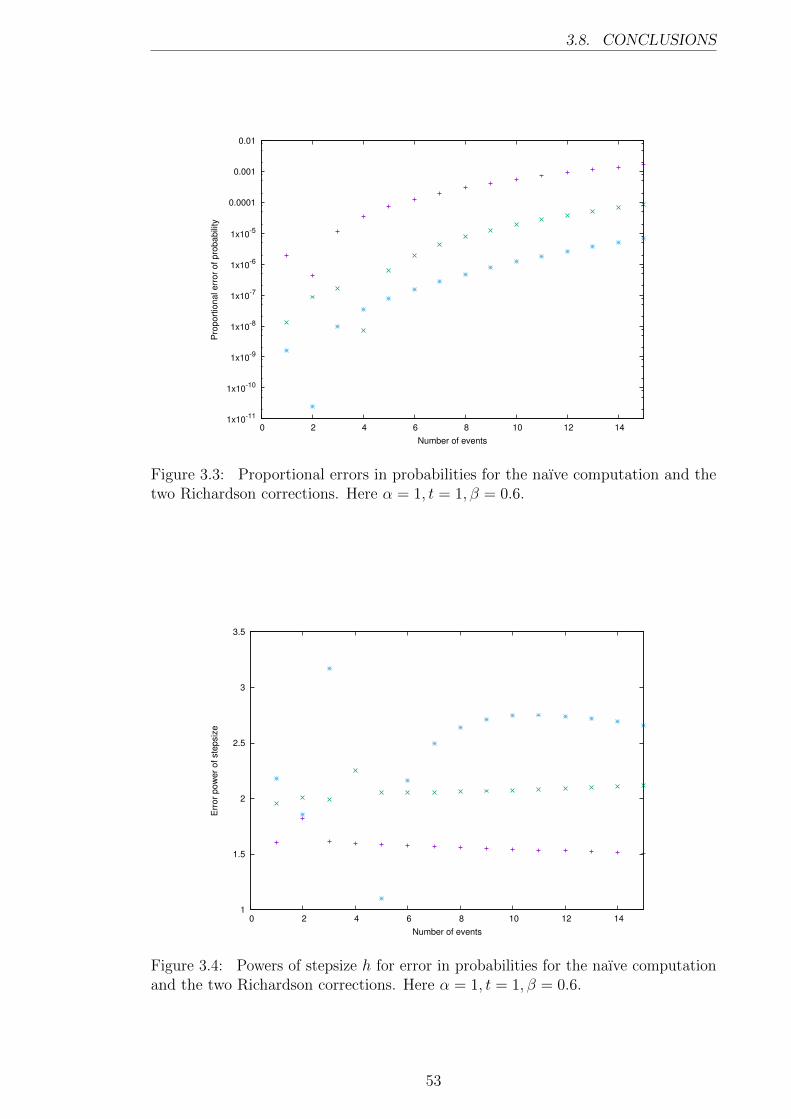
3.8. CONCLUSIONS

1x10-11

1x10-10

1x10-9

1x10-8

1x10-7

1x10-6

1x10-5

0.0001

0.001

0.01

0 2 4 6 8 10 12 14

Pro

port

ional err

or

of pro

babili

ty

Number of events


1

1.5

2

2.5

3

3.5

0 2 4 6 8 10 12 14

Err

or

pow

er

of ste

psiz

e

Number of events

Figure 3.4: Powers of stepsize h for error in probabilities for the naıve computationand the two Richardson corrections. Here α = 1, t = 1, β = 0.6.

53


1x10-8

1x10-7

1x10-6

1x10-5

0.0001

0.001

0.01

0 2 4 6 8 10 12 14

Pro

port

ional err

or

of pro

babili

ty

Number of events


54

Part II

Pre-Match Forecasting Models

and Algorithmic Trading

55

The second part of this thesis builds on the results derived in the first part to

derive two families of pre-match forecasting models and test them in an automated

trading (betting) strategy.

The first model uses the Weibull-based renewal process to build a team-based

model. We adopt the same approach used in the literature and break team strength

in an attack and defence parameter. The improvement introduced by the new

distribution has been found to be significant and positive returns were generated.

The material presented here was turned into a paper submitted to the International

Journal of Forecasting in October 2015.

The second Chapter uses players information collected in our database to derive

a player-based model, again using the Weibull renewal process. The predictive power

of the model was compared to bookmakers’ predictions and also tested in the same

betting strategy. Other application of the model are described. The results described

in this chapter will be submitted to the Journal of the Royal Statistical Society:

Series A (Statistics in Society) in March 2016.

57

CHAPTER

FOUR

A BIVARIATE WEIBULL COUNT MODEL FOR

ASSOCIATION FOOTBALL SCORES

abstract

This Chapter presents a forecasting model for association football scores. The

model uses a Weibull-inter-arrival times based count process and a copula to produce

a bivariate distribution for the number of goals scored by the home and away teams

in a match. We test the model against a variety of alternative models, including the

simpler Poisson distribution-based model and an independent version of our model.

The out-of-sample performance of our methodology is illustrated in a Kelly-type

betting strategy that is applied to the pre-match Win/Draw/Loss market and to

the Over/Under 2.5 goals market. The new model provides an improved fit to data

compared to previous models and results in positive returns to betting.

4.1 Introduction

Since the seminal paper by Maher (1982), much effort has been invested in

modelling the probability distribution of scores in association football. Maher’s

model assumes that the numbers of goals scored by each team in a football match

follow independent Poisson processes, and that the rates at which the teams can

expect to score goals are functions of the ability of the two teams to attack and

defend. Subsequent efforts have enhanced the Maher model in a variety of directions.

Dixon and Coles (1997) make two enhancements to Maher’s model: first, they allow

for dependence between the goals scored by the two teams and second, they address

the dynamic nature of teams’ abilities by using a time-decay function in the likelihood

so that more recent results affect a team’s estimated strength parameters more than

results further in the past. Rue and Salvesen (2000) address the dynamic nature of

teams’ abilities in a Bayesian framework, as does Owen (2011). Karlis and Ntzoufras

(2003) use a bivariate Poisson model with diagonal inflation so that the probabilities

59

CHAPTER 4. A BIVARIATE WEIBULL COUNT MODEL FOR ASSOCIATIONFOOTBALL SCORES

of draw scores are more than would be the case under the simple independent Poisson

model. Most recently Koopman and Lit (2015) use a state space model to allow

team strengths to vary stochastically with time.

These models all assume the basic scoring pattern in football follows a (time-

homogeneous) Poisson process. Perhaps this assumption is made more out of

convenience since, other than the negative binomial distribution, there are surprisingly

few natural alternatives.

Here, we propose using a count process derived when the inter-arrival times are

assumed to follow an independent and identically distributed Weibull distribution.

We refer to this model as the Weibull count distribution and, until recently, the form

of the distribution for the count process generated by non-exponential inter-arrival

times was not known. However, using the techniques discussed in Chapter 3 and the

references therein, new, more general, count process models can now be adopted.

The choice of the Weibull distribution is justified in Section 4.2. In addition to using

a Weibull count model we allow for dependence between the goals scored by the

two teams by employing a copula to generate a bivariate distribution allowing for

positive or negative dependence.

Our objective in this chapter is to build a model for the goals scored by the two

teams in a football match. Our model can be used to construct the probabilities of

score-lines in football matches and hence can be employed in betting market analysis

and, for example, to study market efficiency.

The computations and the graphs in this chapter were done with R (R Core Team,

2015) Countr. To speed up the computations, where necessary, parts of the code

were implemented in C++ using the infrastructure provided by Eddelbuettel and

Sanderson (2014).

The remainder of this chapter is structured as follows: in Section 4.2, we study

the distribution of the time between goals using survival analysis and competing risks

techniques. In Section 4.3 we present the Weibull count distribution, our bivariate

model and give our specification for its use when modelling the goals scored by the

two teams in a football match. Results of fitting our model to the last five seasons of

the English Premier League are presented in Section 4.4 and the performance of a

simple Kelly-based betting strategy described in Section 4.4.2. We conclude with

some closing remarks in Section 4.5.

4.2 Analysis of inter-arrival time between goals

4.2.1 Data

We obtained data on the results of matches in the English Premier League for

the five seasons from 2010/11 to 2014/15 inclusive from www.football-data.co.uk

(1900 games). The data also includes time of goals (in minutes) and pre-match odds

60

www.football-data.co.uk

4.2. ANALYSIS OF INTER-ARRIVAL TIME BETWEEN GOALS

from several bookmakers for the 1X2 (win, draw, lose) market and the over-under

2.5 goals market.

4.2.2 Time to first goal

We start by considering the the distribution of the time to first goal (the event).

We generalise the simplified situation studied in Nevo and Ritov (2013) to a more

realistic competing risks situation where the distribution of time to first goal is

studied together with the type of goal (home or away goal). The competing risks

process is described by the stochastic process (Xt)t∈[0,τ ] attached to Figure 4.1 where

τ can be thought of as the time (since kick-off) of the final whistle.

Figure 4.1: Time to first goal as a competing risks with scoring intensities α1(t)(home) and α2(t) (away).

(Xt)t∈[0,τ ], Xt ∈ {0, 1, 2} simply denotes the state of the match at time t ≥ 0 until

the first goal is scored at time T . Xt equals 0 (state 0− 0 in Figure 4.1 is coded 0

here) if the match is still scoreless at time t. The two potential competing events are

coded 1 (Xt equals 1 if a home goal has occured in [0, t] and hence the match score

would be 1− 0) and 2 (Xt equals 2 if an away goal has occured in [0, t] and hence

the match score would be 0− 1). In association football, all matches starts after the

referee blows the kick-off whistle and the score is 0− 0 at minute 0′ and hence

P(X0 = 0) = 1

The competing risks process moves out of the initial state 0 when a goal is scored at

time T and hence T can be defined as the period of time the match is goalless. In

formula,

T := inf t > 0|Xt 6= 0

T is often called the survival time or failure time (in the survival analysis literature).

If no goal is scored at the final whistle, the match is called ’censored’. We assume that

the match is randomly censored and that its censoring distribution is independent

61


of the distribution of T . This is a reasonable assumption in football as we do not

expect the referee to compute the additional time based on the time of goals or the

current score 1.

The key quantities when analysing competing risks data are the cause-specific

hazards αk(t), k = 1, 2 (team intensity of scoring) defined by

αk(t) = lim∆t→∞

P(t ≤ T < t+ ∆t , XT = k | T ≥ t)

∆t

(4.1)

Football fans can think about the cause-specific hazard as the probability that next

attack is successful (end up in a goal) for the associated team when the score is

still 0-0. The cause specific hazard contains all relevant information that can be

obtained from the data and anything that can be derived uniquely from the cause

specific hazard can be estimated. We also define the cumulative cause specific hazards

Ak(t) =∫ t

0α(u)du. Intuitively, the couple (hazard, cumulative hazard) can be seen

as an equivalent to the couple (density, cumulative distribution functions) and they

both share some properties. Similar to a density function, the hazard αks can be

virtually any nonnegative function. Besides, such as the cumulative distribution

function, the cumulative hazard function can be estimated straightforwardly from

the observed data (using counting process theory and the Nelson-Aalen estimator,

see for example (Andersen et al., 2012)). The hazard can then be recovered using

kernel-based methods as explained in (Muller and Wang, 1994). When estimating

the hazard for one team, the times to the goal scored by the other team are treated

as censored events. As commented by (Putter et al., 2007), this approach is correct

to estimate the cause-specific hazard but special care is needed when computing the

associated scoring probabilities. We refer interested readers to (Putter et al., 2007,

Section 3.1).

Figure 4.2 shows the nonparametric estimated scoring intensities (using the

muhaz() routine from the package with the same name (original by Kenneth Hess

and port by R. Gentleman, 2014) for the first goal together with two parametric

models : an exponential and a Weibull model with hazard function:

α(t) = λctc−1

with λ ∈ (0,+∞) being the scale parameter and c ∈ (0,∞) the shape parameter. The

hazard is monotonically increasing for c > 1, monotonically decreasing for c < 1, and

constant (and equal to λ) when c = 1 (the exponential case). The parametrisation

adopted here is the one used is (McShane et al., 2008) and is known as the proportional

hazard parametrisation. Figure 4.2 shows clearly that the exponential hazard is

not appropriate. It fails to catch the time-varying effect of the hazard and rather

estimates the ’average’ effect over time. The Weibull model describes the data

1In some sense, it is equivalent to assume a ’fair’ (not corrupted) referee

62

4.2. ANALYSIS OF INTER-ARRIVAL TIME BETWEEN GOALS

Distribution Deviance Parameters AIC

exponential 10593 1 10595Weibull 10564 2 10568

Table 4.1: Goodness of fit sum-mary for hazard of first goal forthe home team α1(t). Likelihoodratio test = 28.74 (p-value = 8.24 ·10−8, degrees of freedom (df) = 1).

Distribution Deviance Parameters AIC

exponential 8084 1 8086Weibull 8077 2 8081

Table 4.2: Goodness of fit sum-mary for hazard of first goal forthe away team α2(t). Likelihoodratio test = 7.70 (p-value = 5.52 ·10−3, df = 1).

0 20 40 60 80

0.01

20.

014

0.01

60.

018

0.02

0

time (min)

Haz

ard

0 10 20 30 40 50 60 70 80 90

Kernel density estimateexpweibull

0 20 40 60 80

0.00

80.

009

0.01

00.

011

0.01

20.

013

time (min)

Haz

ard

0 10 20 30 40 50 60 70 80 90

Kernel density estimateexpweibull

Figure 4.2: Scoring intensity for time to first goal by the home team (left) and theaway team (right).

relatively better as summarised in Tables 4.1 and 4.2 (at least for the first 60 minutes)

but fails to catch the subsequent decline in hazard seen in the data. In fact, the

Weibull distribution is either increasing or decreasing and hence cannot catch all

aspect of data generated from a non-monotonic hazard. At least one extra parameter

is needed to accommodate for that. Possible candidates distribution are for example

the generalised gamma (Cox et al., 2007) or the generalised F distribution (Cox, 2008).

A football model using a counting process based on generalised-gamma inter-arrival

times is an on-going research project but in this Chapter, we will focus on the Weibull

case.

4.2.3 Time to next goals

Time to next goals are slightly more challenging to study as they depend on time of

previous goals. We can still fit competing risks models with delayed entry time as explained

in Putter et al. (2007) or more generally a multi-state model which can be seen as a series

of nested competing risks experiments. One example is given in Figure 4.3 where we stop

following the game if the total number of goals is larger than 2.5 (3 or more).

The cumulative hazard for each transition can still be estimated nonparametrically

using the Nelson-Aalen estimators and the transition probabilities

63


Figure 4.3: Scoring process for the three first goals in a football match described bya multi-state model. Each circle represents a state of the match given by a scoreline.Arrows represent the possible transitions from one state to another. When the scoreis x-y, x is always the home team’s goals and y the away team’s goals. Thus a move’upwards’ on the diagram represents a home team goal and a move ’downwards’represents an away team goal.

Plj(s, t) = P(Xt = j|Xs = l, Past) can be computed in closed form if we are ready to

make the markov assumption for the process (Xt)t∈[0,τ ] using the Aalen-Johansen estimator

(Aalen and Johansen, 1978). Such model has been fitted to our data and the results are

summarised in Tables 4.3 and 4.4.

Globally, the Weibull model has been found to better describe the different transitions.

It is also worth noting that the few transitions where the Weibull has not been preferred

to the Exponential are ’rare’ events (not many transitions observed in our data) and hence

the result should be interpreted with care. The analysis of football data using multi-state

models is an interesting area of research and will be the subject of a future publication. It

was briefly introduced here to justify the merit of the use of Weibull distribution for the

inter-arrival time of goals.

64

4.3. A BIVARIATE WEIBULL COUNT PROCESS MODEL

Transition Distribution Deviance Parameters AIC LR-test/p-value

1 exponential 10593 1 10595 28.740-0 → 1-0 Weibull 10564 2 10568 8.24 · 10−8



7 exponential 2072 1 2074 0.0642-0 → 3-0 Weibull 2072 2 2076 8 · 10−1



Table 4.3: Goodness of fit summary for hazard of first three goals for the home team.In all the previous likelihood ratio tests the degrees of freedom are equal to one.

Transition Distribution Deviance Parameters AIC LR-test/p-value







Table 4.4: Goodness of fit summary for hazard of first three goals for the away team.In all the previous likelihood ratio tests the degrees of freedom are equal to one.

4.3 A Bivariate Weibull count process model

4.3.1 The Weibull count process model

McShane et al. (2008) first derived the probability distribution of the number of events

occurring in a count process driven by independent and identically distributed Weibull

inter-arrival times (this process is also known as a Weibull renewal process). They do so

by using a Taylor series expansion of the Weibull density, and expanding the exponential

components of the formula. They name the resulting count process the ‘Weibull count

model ’ and its probability mass function is given by

P(X(t) = x) =

∞∑j=x

(−1)x+j(λtc)jαxjΓ(cj + 1)

, (4.2)

where α0j = Γ(cj + 1)/Γ(j + 1), j = 0, 1, 2, . . . , and αx+1

j =∑j−1

m=x αxmΓ(cj − cm+ 1)/Γ(j −

m+1), for x = 0, 1, 2, . . . , for j = x+1, x+2, x+3, . . . . Alternative methods for computing

65


0 1 2 3 4 5 6

Home goals

Den

sity

0.0

0.1

0.2

0.3

0.4

0 1 2 3 4 5 6

Away goals

Den

sity

0.0

0.1

0.2

0.3

0.4

Fitted Weibull count distribution

Fitted Poisson distribution

Observed frequency

Figure 4.4: Histograms of home goals (left) and away goals (right) with the fittedPoisson and Weibull count models. The estimated parameters (for the weibull models)are, for the home team, λH = 1.50 (0.04), cH = 1.56 (0.03) and for the away team,λA = 1.10 (0.03) and cA = 0.85 (0.04), where the figures in parentheses are standarderrors.

the count probabilities have been described in Chapter 3 but the series expansion (with

Euler-van-Wijngaarden transformations) has been found to be the fastest and is the one

used here. All computation methods are collected in the package Countr available from

the Comprehensive R Archive Network.

Here, the observation unit is the match which we take as having a duration of 1 time

unit. The rate, λ, is thus the scoring rate per match.

Figure 4.4 shows the Weibull count model and the Poisson distribution fitted to the

goals scored by the home team (left) and the away team (right) in matches played in the

English Premier League during the five seasons from 2010-11 to 2014–15. Also shown

are the density histograms of home goals and away goals. Eyeballing the fit of the two

distributions suggests that the Weibull count model and the Poisson distribution provide

similar goodness-of-fit for home goals (although slightly better for the Weibull count

especially for the 0 count), whereas for away goals, it is clear that the Weibull count model

is an improvement. The χ2 goodness-of-fit test statistics for the fitted models shown in

Table 4.5 support this. In fact, they suggest that the Poisson distribution is not adequate

for either home or away goals, while the Weibull count model is appropriate.

Table 4.5: χ2 goodness-of-fit test statistics for the fitted Weibull count model andPoisson distribution to home goals and away goals.

Home Goals Away Goals

χ2 df p-value χ2 df p-valueWeibull count model 7.65 4 0.10 6.59 4 0.16Poisson distribution 13.23 5 0.002 23.5 5 0.0002

We now present a bivariate distribution based on the Weibull count model and include

some modifications that can be used for forecasting the results of football matches.

66

4.3. A BIVARIATE WEIBULL COUNT PROCESS MODEL

4.3.2 Using a copula to generate a bivariate model

The existence of some sort of dependence between the goals scored by two teams in a

football match is widely accepted. However, the exact specification of the dependence is less

clear. For example, Dixon and Coles (1997) find evidence of dependence by studying the

difference in the empirical joint distribution of goals scored by the two teams and the implied

joint distribution under the hypothesis that the two random variables are independent

(i.e. the product of the marginal distributions). Having confirmed the distributions are

not independent, they impose an ad hoc correction to their bivariate Poisson distribution.

Karlis and Ntzoufras (2003) use a diagonally inflated distribution to account for the fact

that draw results are observed more frequently than they would be under the bivariate

Poisson model (although only positive dependence can be captured by the bivariate Poisson

distribution). Here, we follow McHale and Scarf (2011) who choose to allow for any

potential dependence between the goals scored by the two teams by using a copula to ‘glue’

together the two marginal distributions of goals scored.

A copula, C, is a multivariate distribution with all univariate marginal distributions

being uniform on the unit interval, [0, 1]. In other words, C is the distribution of a random

vector with uniform marginals. The power of using a copula approach for modelling

dependence comes from a theorem due to Sklar (See for example Carley and Taylor (2002)

for a recent proof.) that states that the joint cumulative distribution function F of any

pair of random variables (Y1, Y2) may be written in the form

F (y1, y2) = C(F1(y1), F2(y2)), (y1, y2) ∈ <2,

where F1 and F2 are marginal cumulative distribution functions and C is a copula.

Here we want to join two marginal distributions and in this bivariate case, there are a

plethora of copulas to choose from. We choose the Frank’s copula which belongs to the

flexible family of Archimedean copulas and allows for the full range of dependence so that

the correlation can range from −1 to 1. The Frank copula is given by

C(u, v) = −1

κln

(1 +

(e−κu − 1)(e−κv − 1)

e−κ − 1

),

where κ ∈ < is the dependence parameter.

To construct our bivariate Weibull count model we use the Weibull count probability

mass function given by (4.2) to first calculate the cumulative distribution functions,

F1(y1;λ1) and F2(y2;λ2). Using the copula C(u, v;κ) to glue these marginals together,

the likelihood function for the parameter vector (λ1, c1, λ2, c2, κ) given the ith pair of

observations (y1i, y2i) is

L(λ1, c1, λ2, c2, κ; y1i, y2i) = P(Y1 = y1i, Y2 = y2i)

= C(F1(y1i), F2(y2i))− C(F1(y1i − 1), F2(y2i))−

C(F1(y1i), F2(y2i − 1)) + C(F1(y1i − 1), F2(y2i − 1)).

(4.3)

The log-likelihood, `(λ1, c1, λ2, c2, κ; y1,y2) =∑n

i=1 logL, for a sample of n football matches

67


can be maximised using standard numerical optimisation routines.

We note that Frank’s copula nests the independence case (κ = 0) so that a test of

whether κ is equal to 0 is equivalent to testing the assumption of independence.

4.3.3 A Model for goals

Since Maher (1982) first gave his specification for modelling the goals scored by the two

teams in a football match, many researchers have followed suit. Adapting the specification

to our bivariate model is simple due to the presence of the rate parameter, λ, in the

distribution function given in equation (4.2). As in Maher (1982) we let the rate parameter

for home team i playing against away team j (λHi,j) be

log(λHi,j) = αi + βj + γ,

where αi is the attack strength (the higher the value of α, the stronger is the attack) of

team i, βj is the defence strength (the smaller the value of β, the stronger is the defence)

of team j and γ is a home advantage parameter. The away team’s scoring rate (λAi,j) is

given by

log(λAi,j) = αj + βi.

To prevent the model from being over-parameterised, we impose the contraint

1

n

n∑i=1

αi = 0

where n is the total number of teams in the data.

The above model is static in that the team strength parameters are not allowed to

vary with time. This is not a good approximation. For example, Baker and McHale (2015)

present a time varying model for team strengths and find that the strengths do indeed vary

over time as, for example, teams buy and sell players, injuries occur and runs of good and

bad form happen. In the forecasting literature there have been two approaches to allowing

time-varying team strengths.

First, one can build a model in which the team strengths are assumed to vary stochasti-

cally, such as in Crowder et al. (2002), Owen (2011) or Koopman and Lit (2015). However,

on top of being computationally intensive and fraught with numerical instabilities, this

approach needs a model for their evolution, such as the autogressive model in Crowder

et al. (2002) and Koopman and Lit (2015) and the normal prior in Owen (2011). This

model is necessarily ad hoc and cannot be validated in practice because the estimated

parameters (the team strengths) are not ‘observable’ quantities.

Second, one can adopt a time decay factor in the likelihood function so that more recent

matches have greater weight in estimating the team strength parameters than matches

further in the past. Implicitly one is assuming that the results of each team are indicative

of that team’s changing strength — a seemingly intuitive and reasonable assumption to

make. This is the approach adopted in Dixon and Coles (1997) and is how we deal with

the problem here.

68

4.4. RESULTS

Using an exponential weighting function, our ‘pseudo-likelihood’, L, at time t is given

by

Lt(κ, c, α, β) =∏k∈At

e−ξ(t−tk)L,

where tk is the time when match k was played, At = {k : tk < t} is the subset of all matches

played up to, but not including, time t and L is as given in equation (4.3). The parameter

ξ cannot be estimated by maximising the likelihood. Dixon and Coles (1997) select the ξ

that maximises

S(ξ) =N∑k=1

(δHk log pHk + δAk log pAk + δDk log pDk ),

where δHk = 1 if match k is a home win (else δHk = 0), and pHk , pAk and pDk are the maximum

likelihood estimates of a home win, an away win and draw respectively. We modify this

approach as our model is perhaps ‘wasted’ testing it against only the 1X2 (home win, draw,

away win) market. Rather, we choose ξ to maximise the following objective function which

includes the over-under 2.5 goals market

T (ξ) =

N∑k=1

(δHk log pHk + δAk log pAk + δDk log pDk + γO2.5k log pO2.5

k + γU2.5k log pU2.5

k ), (4.4)

where γO2.5k = 1 if there are more than 2.5 goals in match k and γU2.5

k = 1 if there are

fewer than 2.5 goals in match k and pO2.5k and pU2.5

k are the model implied probabilities of

there being more than or less than 2.5 goals in match k. Figure 4.5 shows a plot of (4.4) as

ξ varies from 0 to 0.008 and there is a clear maximum at ξ = 0.002 and this is the value we

use throughout. Following Dixon and Coles (1997) we use a half-week as the unit of time.

They estimate a value of 0.0065 which is of the same order of magnitude of our estimated

value of ξ.

4.4 Results

Before using our model as the basis of a betting strategy, we first take a look at the

estimated team strengths and some model fit diagnostics.

4.4.1 Estimated team strengths

To show our results we fitted the model to all five seasons of results data to the end

of the 2014–15 season. The estimated distribution parameters c in equation (4.2) are

cH = 1.070 (7.29×10−4) for the home team and cA = 1.010 (8.54×10−4) for the away team

(standard errors in parentheses). The estimated value of the dependence parameter in the

copula is κ = −0.39 (3.53× 10−3), so that the value of Kendall’s τ is -0.043 suggesting a

negative (and statistically significant) dependence. Lastly, the estimated home advantage

is γ = 0.33 (8.93× 10−4).

The standard errors have been computed using the boostrap method described in Efron

(1992) in which 500 replicate datasets of identical size to the original data were generated

by sampling from the original data with replacement. Note that if one tries to compute the

69


0.000 0.002 0.004 0.006 0.008

−31

6.4

−31

6.2

−31

6.0

−31

5.8

−31

5.6

−31

5.4

Time−Decay ξ

T(ξ

)

Figure 4.5: Selecting the decay factor ξ by maximizing the objective function T (ξ)defined in (4.4). The maximum occurs at ξ = 0.002

standard errors using the pseudo-likelihood misleading results may be produced. In fact,

teams who competed only for the first seasons in the Premier League (Birmingham City

and Blackpool for example) will have large standard errors value (due to the weighting

scheme applied). The standard errors reported in Table 4.6 where therefore computed using

the ’true’ likelihood instead of the ’pseudo’ one. The estimated team strength parameters,

α (attack) and β (defence), for our model are in agreement with what football fans can

expect. Teams who are know to perform well (Arsenal, Manchester City, Chelsea, ...) have

the largest attacking and the smallest (negative) defensive coefficients.

4.4.2 Model diagnostics and a Kelly betting strategy

We discuss both in-sample and out-of-sample performance of our main model and

compare it with the performance of three other models, an independent Poisson model, an

independent Weibull count model and a Frank copula-induced bivariate Poisson model.

Using these three models as benchmarks enables us to gauge where any out-performance may

be originating (for example, an improvement in goodness-of-fit may come from modelling

the dependence structure using a copula or it may come from modelling the counts using a

Weibull count model rather than a Poisson distribution).

Table 4.7 shows the log-likelihood, the number of model parameters and the AIC

for each of the four models under consideration. Although the copula-induced bivariate

Weibull count model has more parameters, it is the best fitting model based on the AIC. It

is noteworthy that the change from Poisson to Weibull count distribution improves the

AIC by approximately 3, and the change from independence to copula-induced dependence

improves the AIC by approximately 4. As such, it looks like the overall improvement of our

model comes equally from the copula-based dependence and from the use of the Weibull

70

4.4. RESULTS

Table 4.6: Estimated team strength parameters, based on the full five seasons matches.Larger α’s indicate stronger attack, smaller β’s stronger defence.

Team α (s.e.) β (s.e.)Arsenal 0.410 (0.055) -0.150 (0.074)Aston Villa -0.157 (0.070) 0.198 (0.065)Birmingham City -0.291 (0.160) 0.147 (0.135)Blackburn Rovers -0.032 (0.101) 0.343 (0.090)Blackpool 0.130 (0.132) 0.471 (0.118)Bolton Wanderers 0.004 (0.100) 0.313 (0.092)Burnley -0.486 (0.183) 0.076 (0.140)Cardiff City -0.344 (0.171) 0.412 (0.120)Chelsea 0.391 (0.054) -0.305 (0.081)Crystal Palace -0.138 (0.109) 0.015 (0.104)Everton 0.103 (0.062) -0.130 (0.073)Fulham -0.017 (0.073) 0.199 (0.071)Hull City -0.258 (0.116) 0.067 (0.102)Leicester City 0.024 (0.143) 0.140 (0.137)Liverpool 0.328 (0.056) -0.063 (0.071)Manchester City 0.529 (0.051) -0.329 (0.080)Manchester United 0.470 (0.053) -0.212 (0.076)Newcastle United 0.024 (0.065) 0.205 (0.062)Norwich City -0.154 (0.089) 0.236 (0.078)Queens Park Rangers -0.203 (0.056) 0.302 (0.056)Reading -0.088 (0.088) 0.392 (0.078)Southampton 0.123 (0.079) -0.044 (0.089)Stoke City -0.130 (0.069) -0.011 (0.069)Sunderland -0.161 (0.070) 0.086 (0.066)Swansea City 0.020 (0.072) 0.052 (0.075)Tottenham Hotspur 0.236 (0.058) -0.023 (0.070)West Bromwich Albion -0.006 (0.065) 0.174 (0.065)West Ham United -0.089 (0.076) 0.120 (0.072)Wigan Athletic -0.116 (0.089) 0.282 (0.077)Wolverhampton Wanderers -0.119 (0.106) 0.411 (0.088)

count distribution.

Table 4.7: Comparison of the four models for football scores fitted (in-sample) to thePremier League data.

log-likelihood params AICCopula Weibull Count Model -5471.97 64 11071.93

Copula Poison Model -5474.86 62 11073.72Independent Weibull Count Model -5475.19 63 11076.38

Independent Poisson Model -5478.10 61 11078.21

We now test the same four models against the betting market. There is a vast array

of work in the economics literature examining the efficiency of the betting market on

football, and, on the whole, there is agreement that the market is efficient in that it is

not possible to accrue ‘superior’ returns (see, for example, Snowberg and Wolfers (2010)).

71


Thus, comparing the probabilities implied in the betting market with those produced by

the model is a simple, but informative guide to the model’s effectiveness. Figure 4.6 shows

scatter plots of the average bookmaker implied probabilities for home win, draw and away

win versus the corresponding model probabilities for the 2014–15 season. In general there

is a high level of agreement between the two, though for high probability events (strong

favourites) there is some tendency for the market to estimate a higher probability than

the model. This is likely to be evidence of the famous ‘longshot bias’ — a phenomenon

witnessed across many sports and many betting markets whereby bettors accept poor value

odds on strong favourites (see, for example, Direr (2013)).

0.0 0.2 0.4 0.6 0.8 1.0

0.0

0.2

0.4

0.6

0.8

1.0

Pr(home win), average odds

Pr(

hom

e w

in),

mod

el

0.0 0.2 0.4 0.6 0.8 1.0

0.0

0.2

0.4

0.6

0.8

1.0

Pr(draw), average odds

Pr(

draw

win

), m

odel

0.0 0.2 0.4 0.6 0.8 1.0

0.0

0.2

0.4

0.6

0.8

1.0

Pr(away win), average oddsP

r(aw

ay w

in),

mod

el

Figure 4.6: Bookmaker implied probabilities (rescaled to sum to 1) versus modelprobabilities for home win, draw and away win.

Figure 4.7 shows scatter plots of the average bookmaker probabilities of over (under) 2.5

goals1 in the match versus the corresponding model implied probabilities for the 2014–15

season. There seems to be a much weaker relationship between the model and the market.

Further, there is some evidence that the market assigns a higher probability to more than

2.5 goals than the model does. From conversations with industry traders, this may be

because of a bias not studied in the academic literature, in that bettors prefer to bet on an

exciting match with lots of goals, than to be pessimistic and bet on a dull match with few

goals.

0.0 0.2 0.4 0.6 0.8 1.0

0.0

0.2

0.4

0.6

0.8

1.0

Pr(over 2.5 goals), average odds

Pr(

over

2.5

goa

ls),

mod

el

0.0 0.2 0.4 0.6 0.8 1.0

0.0

0.2

0.4

0.6

0.8

1.0

Pr(under 2.5 goals), average odds

Pr(

unde

r 2.

5 go

als)

, mod

el

Figure 4.7: Bookmaker implied probabilities (rescaled to sum to 1) versus modelprobabilities for over/under 2.5 goals.

We now turn to the ‘true test’ of our forecasting model: betting. Our betting simulation

is out-of-sample: team strengths are estimated using results prior to the match to be bet

1The over-under 2.5 goals market is a popular bet for punters in which the bookmaker offersodds on there being more than, or less than, 2.5 goals in the match, in total.

72

4.4. RESULTS

on. We use the first four and a half seasons results leaving the final 190 games of the

2014–15 season to bet on. After each week of matches have been played, we re-estimate

the team strengths by dropping the first week’s matches and adding the ‘new’ week’s

set of results. As a consequence of the efficient markets hypothesis, we would consider a

return of near the market over-round as evidence that a model is working well. We use the

average odds available on two markets: the 1X2 (home win, draw, away win) market, and

the over-under 2.5 goals market. During the last half of the 2014–15 season, the average

over-rounds on the two markets were 4.9% and 5.7% respectively. By testing our model

against the over-under market we are gaining an understanding of the model’s performance

in predicting what it was designed to forecast - goals. If we were to test the model against

only the 1X2 market, we would be disregarding the main output from the model - the

probabilities of each and every possible scoreline.

Our investment strategy is based on the Kelly Criterion (Kelly, 1956). The Kelly

criterion is borne from a desire to maximise long-run log-utility and it results in an

investment strategy where the bettor invests a fraction f of his overall wealth

f =(b+ 1)p− 1

b,

where p is the bettor’s estimate of the probability of an event (e.g. the home team winning

the game), and b is the (fractional) odds offered by the bookmaker (where 1/(b+ 1) can be

interpreted loosely as the bookmaker’s implied probability of the event occurring).

We allow a maximum of 10 units per bet and use the Kelly criterion to decide on what

fraction of our 10 units is staked. Effectively we reset our bankroll to 10 after each bet.

An additional ‘protection’ was also introduced: we restrict ourselves to ‘quality bets’ when

the expected value of any bet is above a threshold. For each game, there are five possible

events to bet on: home win, draw, away win, over 2.5 goals and under 2.5 goals. For event

type A, we only bet if

EV (A) = P (A)×Odds(A)− 1 > t,

where t is a threshold parameter and effectively serves to protect the investment strategy

when the bookmaker knows more than the model. Experimentation led us to use t = 0.15

which is a good compromise between betting too much (and losing) and placing a reasonable

number of bets. Table 4.8 shows the out-of-sample returns to 1X2 betting on matches in

the final half (190 games) of the 2014–15 season and Table 4.9 shows the out-of-sample

returns to betting on the over-under 2.5 goals market for the same 190 games.

Table 4.8: Summary of results when betting on the 1X2 market.

Model Number Number of Gross Net Total Totalof bets winning bets return return staked return

Copula Weibull Count 34 10 35.65 1.55 34.10 4.6 %Independent Weibull Count 44 11 41.41 -0.44 41.86 -1.1 %

Copula Poisson Model 45 11 40.38 -1.86 42.24 -4.4 %Independent Poisson Model 45 10 37.22 -2.81 40.03 -7 %

In both cases the copula Weibull count model produces the highest returns: 4.6% in

73


Table 4.9: Summary of results when betting on the over-under 2.5 goals market.

Model Number Number of Gross Net Total Totalof bets winning bets return return staked return

Copula Weibull Count Model 23 15 51.81 12.03 39.78 30 %Copula Poisson Model 21 13 46.58 10.54 36.04 29 %

Independent Poisson Model 22 13 48.16 9.88 38.28 26 %Independent Weibull Model 26 15 53.41 8.58 44.83 19 %

the case of the 1X2 market and 30% in the over-under market. In general, the returns are

lower for the 1X2 market. This may be because the 1X2 market is more ‘efficient’. Perhaps

this is because traders have better expertise and more experience of compiling 1X2 odds

because it is the oldest, and most commonly bet on market.

We also note the seemingly small number of games bet on. This is not unusual and

in fact, we bet on a relatively high proportion of games. For example, Koopman and Lit

(2015) place just 50 bets over two seasons, equating to a bet rate of 6.6 per game. Here,

we have a bet rate of 34/190 = 17.9% per game on the 1X2 market and 23/190 = 12.1%

on the over-under 2.5 goals market.

Obtaining returns that are superior and positive in both the 1X2 and over-under 2.5

markets, is interesting for two reasons. First, we take the results as validation of our model,

and second, and more profoundly, there are implications for market efficiency, which may

be the subject of future research.

4.5 Discussion

In this chapter we have studied a new model for bivariate counts to predict the score

distribution in football matches. Our model assumes that the distribution of inter-arrival

time for goals is Weibull, rather than exponential (the latter is implied when using the

Poisson distribution). We induce dependency between the two marginals using a Frank

copula. We test this bivariate Weibull count model against three alternative models both

in-sample and out-of-sample and the bivariate Weibull count model provides a superior fit

to results data from the English Premier League.

Perhaps most interesting is the finding that our model attains positive returns in

both the 1X2 and over-under 2.5 goals betting markets. However, it is worth noting that

although we can ‘beat the bookmakers’, we are picking and choosing a relatively small

number of matches to bet on. A bookmaker must produce competitive odds for an entire

league fixture list. To do so is a more challenging task and requires intimate knowledge

of the leagues, teams and players involved. Hence, in the betting industry, bookmakers

remain reliant on a system in which both statistical models and traders work in tandem to

produce odds. However, the model presented here may prove to be of use to bookmakers.

For example, we believe that bookmakers estimate a supremacy rating for one team over

another in a match and an expected number of goals in the match. Bookmakers could

use these two variables, which are based on intimate knowledge of the form of the teams

and the players actually playing for each team, as inputs to our model. The 1X2 markets

74

4.5. DISCUSSION

will still be priced the same but by better estimating the goals distribution, more accurate

prices for the subsidiary markets will be produced.

An alternative to our approach to relaxing the (time-homogeneous) Poisson assumption,

is to assume that only the time to first goal (first inter-arrival for each scoring process)

is Weibull distributed and to model the dependence between the two first arrival times

(TH and TA) with an (archimedian) copula (see Tuerlinckx, 2004). Although appealing,

this approach suffers from two major drawbacks. First, identifiability is not guaranteed as

the observable data (min(TH , TA)) does not allow us to verify whether TH and TA are

dependent or independent. An immediate consequence is that the model parameters cannot

be estimated uniquely from the (log)-likelihood (We refer to Kalbfleisch and Prentice (2011,

Section 8.2.4) for a proof and in depth discussion or identifiability). Second, closed formula

for the final bivariate count are only obtained if the Gumbel’s copula is used, which does

not allow to model the full range of dependence. For these reasons, this method was not

pursued here but it maybe the subject of future research.

In the next Chapter, we bridge the gap between the statistical model and traders by

incorporating player skills into our model. Using knowledge on the identity of the players

on each team (and their abilities) should avoid the need for estimating time-varying team

strengths as the key component of the dynamic nature of team strengths is the changing

lineup of the team. If accurate player ratings are used as inputs to the model, such an

approach should produce much improved forecasts as it will better capture the expected

scoring intensities of each team (we refere readers to Chapter 5 to see the answer).

75

CHAPTER

FIVE

A PLAYER BASED MODEL FOR ASSOCIATION

FOOTBALL SCORES

abstract

This Chapter presents a player-based model for football scores which takes into account

the abilities of the players on each team. The advantage of this approach is that the

dynamic nature of team strengths are incorporated into the model. We test our model

against the bookmakers predictions and in a Kelly-type betting strategy that is applied

to the pre-match Win/Draw/Loss market and to the Over/Under goals market. The

new model provides an improved fit to data compared to previous models and results

in significant positive returns to betting. The model is also used to answer some useful

questions related to the ’nature’ of the game.

5.1 Introduction

Models for the predicting the results of football matches are typically based on the

identity of the two teams and estimating each team’s strength (often split into two: attack

strength and defence strength) based on past match results. In recent times the focus

of such models has been on allowing for these strengths to vary with time. For example,

Dixon and Coles (1997) apply a down-weighting in the likelihood function so that matches

played further in the past influence a team’s estimated strength less than matches played

more recently; Baker and McHale (2015) assume team strengths vary deterministically

over a long time period; and Crowder et al. (2002), Owen (2011), and Koopman and Lit

(2015) adopt models that allow the strengths to vary stochastically from match to match.

Although work has been done on allowing team strengths to vary, there has been little

attention paid to why team strengths vary and what the physical mechanism is which

drives these variations in strengths from match to match and season to season. It seems

likely that the reasons for the dynamic nature of team strengths fall into two categories:

first, the identity of the players making up the team varies, and second, the form of the

individual players varies as players go through good and bad patches. We refer to these

mechanisms as ‘line-up’ and ‘form’ respectively. In this chapter we include both of these

77

CHAPTER 5. A PLAYER BASED MODEL FOR ASSOCIATION FOOTBALLSCORES

mechanisms which drive the time-varying team strengths in a model for predicting the

outcome of football matches. We do so by including information on the playing ability

of the players on the pitch for each team. Because our model is driven by the strengths

of those players actually on the pitch, it deals with the first source of variation in team

strengths (‘line-up’), by using information on the line-up of players on the pitch. Further,

we account for the short-term ‘form’ of players by adjusting the long-term ability ratings

using match-by-match ratings of players published in newspapers. Adjusting the long-term

ability ratings using these short-term match ratings therefore deals with the second source

of team strength dynamics: player form.

5.2 Data

The data requirements for our model are non-trivial, and this is perhaps a major reason

for why this type of model has not been published in the past. First, we need the results

data and this was obtained from www.football-data.co.uk for the top tier of football in

England, the Premier League, for the seven and half seasons from 2009-2010 until week 20

of season 2015-2016. Second, we need the identities of the players on the pitch for each

game. This was scraped from the website www.line-ups.com for all the games in our

results data set.

Next, we need to obtain player ability ratings. There are several possibilities and

several authors have produced models for rating players (see, for example, McHale et al.

(2012a)). We refer the reader to Chapter 2 for a detailed description of the players data

used and how it was obtained. Here, we simply provide two further simple tests of whether

the player ratings are likely to be informative in a model for predicting match outcomes.

First, we note that the team with the highest total player ratings goes on to win in 51%

of matches1. Second we use the sum of player ratings for the two teams as covariates in

an ordered logistic regression model for match outcome (the possible outcomes are win,

draw, loss). The results are shown in Table 5.1. The estimated coefficients on the two

player strength variables are strongly statistically significant (the coefficient on the sum of

the ratings for the home team players is larger in magnitude than the sum of the player

ratings for the away team because of the home advantage effect).

Table 5.1: Results of ordinal regression fit to explain match outcome as a function ofthe sum of each team’s player ratings.

Coefficient (s.e.)

Sum of home player ratings 0.177 (0.011)Sum of away player ratings -0.141 (0.011)Threshold 1 1.680Threshold 2 2.918

Although the player ratings from video games are updated each week in recognition

of changing form, as we shall see there is a faster moving short-term effect in a player’s

1Given there are three possible outcomes in football, this is significantly higher than would beexpected if there was no information in the player ratings.

78

www.football-data.co.uk

www.line-ups.com

5.3. A PLAYER-LEVEL MODEL FOR SCORES

performance level which we call player ‘form’. In order to take into account a player’s

form and these short-term changes in a player’s performances, we also use the player

ratings system presented in McHale et al. (2012a) and has been used as the official player

ratings system of the Premier League for the last nine years. A full description of this

player ratings system falls beyond the scope of this chapter and so we provide only a

brief description. For each game of the season, each player on the pitch receives a rating

score based on the actions (passes, tackles, shots, goals, red cards, and so on) he performs

during a match. Some actions are rewarded more highly than others; for example, a cross

is worth more than a pass in the player’s own half. Whilst other actions are negatively

rewarded, such as red cards. These ratings are much more volatile than the video game

ratings discussed above, and are more responsive to good (and bad) runs of form. This is

exactly the characteristics of short-term performance levels that we are looking to capture.

5.3 A Player-level model for scores

Our basic model for the scoreline in a football match is a bivariate Weibull count model

first described in Chapter 4 (Section 4.3) (see also Boshnakov et al. (2016a)).

Following Maher (1982) and others since (for example, Dixon and Coles (1997), and

Koopman and Lit (2015)), the rate parameters in (4.2) are functions of the attack and

defence abilities of the two teams competing. Specifically, the rate parameter for home

team i playing against away team j in match m is given by

log(λim) = αim + βjm + γ, (5.1)

where αim is the attack strength of team i in match m, βjm is the defence strength of team

j in match m and γ is a home advantage parameter. The away team’s scoring rate is given

by

log(λjm) = αjm + βim. (5.2)

Typically, αim and βim are assumed to depend only on the team, and not be a function

of the players abilities playing in match m. We now present our extension to this model so

that player information can be included.

5.3.1 Including player-level information

To incorporate the player ratings in the model there are many specifications possible.

Here we present two options and in each of them, we let the α’s and β’s in (5.1) and (5.2)

be functions of the player ratings. Before discussing any adjustements made to the overall

ratings to account for player form, we present our two basic model specifications. Our first

specification is the ‘simplest’ most intuitive specification, whilst the other specification

is our best performing model allowing for the subtleties of football, and how players in

different positions affect the outcome of a match.

The simple specification is such that for team i in match m playing at home against

79


team j, we let the attack strength of the team be given by

αim = α11∑p=1

Sip/11, (5.3)

where Sip is the overall score of player p of team i and the sum is taken over all players on

team i (p = 1, . . . , 11) in match m and α is a coefficient to be estimated. Similarly we let

defensive strength of the opposition team be given by

βjm = β11∑p=1

Sjp/11, (5.4)

where β is a coefficient to be estimated. This model is extremely simple as it assumes

all players contribute equally to attack and defence. Of course, this may be an over-

simplification since some players specialise in contributing to attack rather than defence,

or vice versa. However, its use here is to demonstrate that the player ratings are indeed

informative and to provide a baseline model for our main model.

Our ‘full’ model makes two key enhancements to the basic model above. First, we allow

for the possibility that players may specialise and not necessarily be as good at defending

as they are at attacking, or vice versa. Second, we allow the contribution of the different

positions on the team to contribute to α and β differently.

To allow the contribution of a player’s ratings to the team’s attack and defence strengths

to vary depending on the playing position of the player, we compute two ratings for each

player. Instead of using the player’s overall rating when calculating both α and β (as in

equations (5.3) and (5.4)), we use the information in the video game databases to compute

(i) a rating for the player’s ability to attack, which we denote by Sp, (and use this when

calculating the team’s α); and (ii) a rating for the player’s ability to defend, which we

denote by Sp, (and use this when calculating the team’s β).

Next, we allow the contribution to the attack and defence strengths of the team to vary

depending on the different positions. We consider five categories of ‘position’: goalkeeper

(gk), centre-backs (cb), full-backs (fb), midfielders (mf) and forwards (fw).

Combining these two refinements, the attacking strength of team i, playing in match

m against team j is given by a weighted average of the attacking ‘strength’ of each line as

follows:

αim =αfwS

fwim + αmf S

mfim + αfbS

fbim + αcbS

cbim + αgkS

gkim

11, (5.5)

where αfw, αmf , αfb, αcb, and αgk are weights to be estimated, and Sfwim , Smfim , Sfbim,

Scbim and Sgkim are the sum of the attacking ratings for the players playing as forwards,

midfielders, full-backs, centre-backs and the goalkeeper respectively, on team i in match m.

Similarly, the defensive strength of team j in the same match is given by

βjm =βfwS

fwjm + βmf S

mfjm + βfbS

fbjm + βcbS

cbjm + βgkS

gkjm

11, (5.6)

where βfw, βmf , βfb, βcb, and βgk are again coefficients to be estimated, and Sfwim , Smfim ,

Sfbim, Scbim and Sgkim are the sum of the defensive scores for the players playing as forwards,

80

5.3. A PLAYER-LEVEL MODEL FOR SCORES

midfielders, full-backs, centre-backs and the goalkeeper respectively, on team j in match m.

The specification adopted in our full model takes into account the formation of the

team since the player’s rating depends on his position and hence on the formation the team

is playing. Further, this specification is also able to account for both: players playing in

unfamiliar positions, and for players to contribute to the attack or defence efforts to lesser

or greater extents depending on their position on the pitch.

Having discussed our two basic model specifications, we now turn our attention to

including player ‘form’ in the model.

5.3.2 Excess performance

The ratings used in the previous Section can be seen as a measure of the players’

long-term ability. An ability is by definition ‘stable’ in time. Even though each players’

overall ability ratings are updated each week by the video game manufacturers, the ratings

score is not particularly sensitive to short-term changes in form. Consider, for example,

the evolution of Jamie Vardy’s overall rating, which is plotted as the solid circles in Figure

5.1. As expected, his good performances in the first half of the 2015-2016 season resulted

in an increase in his overall rating ability, going from 67 to 75.

● ●●●●●●●●●●●●●●●●●●●●●●●●●●●●●

●

●●

●●●●●●●●●●●●●●●●●●●●●●

●●●●●●●●●●●●●●●●● ●●●●●●●●●●●●●●●

●●●●●●●●●●●●●●●●●●●●●●●●●●●●●●●●●●●●●●●●●●●●●●●●●●●●●

●

●●

●●●●●

●●

●●●

●●●●●●●●●●●●●

2012 / 20132012 / 20132012 / 20132012 / 20132012 / 20132012 / 20132012 / 20132012 / 20132012 / 20132012 / 20132012 / 20132012 / 20132012 / 20132012 / 20132012 / 20132012 / 20132012 / 20132012 / 20132012 / 20132012 / 20132012 / 20132012 / 20132012 / 20132012 / 20132012 / 20132012 / 20132012 / 20132012 / 20132012 / 20132012 / 20132012 / 20132012 / 20132012 / 20132012 / 20132012 / 20132012 / 20132012 / 20132012 / 20132012 / 20132012 / 20132012 / 20132012 / 20132012 / 20132012 / 20132012 / 20132012 / 20132012 / 20132012 / 20132012 / 20132012 / 20132012 / 20132012 / 20132012 / 20132012 / 20132012 / 20132012 / 20132012 / 20132012 / 20132012 / 20132012 / 20132012 / 20132012 / 20132012 / 20132012 / 20132012 / 20132012 / 20132012 / 20132012 / 20132012 / 20132012 / 20132012 / 20132012 / 20132012 / 20132012 / 20132012 / 20132012 / 20132012 / 20132012 / 20132012 / 20132012 / 20132012 / 20132012 / 20132012 / 20132012 / 20132012 / 20132012 / 20132012 / 20132012 / 20132012 / 20132012 / 20132012 / 20132012 / 20132012 / 20132012 / 20132012 / 20132012 / 20132012 / 20132012 / 20132012 / 20132012 / 20132012 / 20132012 / 20132012 / 20132012 / 20132012 / 20132012 / 20132012 / 20132012 / 20132012 / 20132012 / 20132012 / 20132012 / 20132012 / 20132012 / 20132012 / 20132012 / 20132012 / 20132012 / 20132012 / 20132012 / 20132012 / 20132012 / 20132012 / 20132012 / 20132012 / 20132012 / 20132012 / 20132012 / 20132012 / 20132012 / 20132012 / 20132012 / 20132012 / 20132012 / 20132012 / 20132012 / 20132012 / 20132012 / 20132012 / 20132012 / 20132012 / 20132012 / 20132012 / 20132012 / 20132012 / 20132012 / 20132012 / 20132012 / 20132012 / 20132012 / 20132012 / 20132012 / 20132012 / 20132012 / 20132012 / 20132012 / 20132012 / 20132012 / 20132012 / 20132012 / 20132012 / 20132012 / 20132012 / 20132012 / 20132012 / 20132012 / 2013 2013 / 20142013 / 20142013 / 20142013 / 20142013 / 20142013 / 20142013 / 20142013 / 20142013 / 20142013 / 20142013 / 20142013 / 20142013 / 20142013 / 20142013 / 20142013 / 20142013 / 20142013 / 20142013 / 20142013 / 20142013 / 20142013 / 20142013 / 20142013 / 20142013 / 20142013 / 20142013 / 20142013 / 20142013 / 20142013 / 20142013 / 20142013 / 20142013 / 20142013 / 20142013 / 20142013 / 20142013 / 20142013 / 20142013 / 20142013 / 20142013 / 20142013 / 20142013 / 20142013 / 20142013 / 20142013 / 20142013 / 20142013 / 20142013 / 20142013 / 20142013 / 20142013 / 20142013 / 20142013 / 20142013 / 20142013 / 20142013 / 20142013 / 20142013 / 20142013 / 20142013 / 20142013 / 20142013 / 20142013 / 20142013 / 20142013 / 20142013 / 20142013 / 20142013 / 20142013 / 20142013 / 20142013 / 20142013 / 20142013 / 20142013 / 20142013 / 20142013 / 20142013 / 20142013 / 20142013 / 20142013 / 20142013 / 20142013 / 20142013 / 20142013 / 20142013 / 20142013 / 20142013 / 20142013 / 20142013 / 20142013 / 20142013 / 20142013 / 20142013 / 20142013 / 20142013 / 20142013 / 20142013 / 20142013 / 20142013 / 20142013 / 20142013 / 20142013 / 20142013 / 20142013 / 20142013 / 20142013 / 20142013 / 20142013 / 20142013 / 20142013 / 20142013 / 20142013 / 20142013 / 20142013 / 20142013 / 20142013 / 20142013 / 20142013 / 20142013 / 20142013 / 20142013 / 20142013 / 20142013 / 20142013 / 20142013 / 20142013 / 20142013 / 20142013 / 20142013 / 20142013 / 20142013 / 20142013 / 20142013 / 20142013 / 20142013 / 20142013 / 20142013 / 20142013 / 20142013 / 20142013 / 20142013 / 20142013 / 20142013 / 20142013 / 20142013 / 20142013 / 20142013 / 20142013 / 20142013 / 20142013 / 20142013 / 20142013 / 20142013 / 20142013 / 20142013 / 20142013 / 20142013 / 20142013 / 20142013 / 20142013 / 20142013 / 20142013 / 20142013 / 20142013 / 20142013 / 2014 2014 / 20152014 / 20152014 / 20152014 / 20152014 / 20152014 / 20152014 / 20152014 / 20152014 / 20152014 / 20152014 / 20152014 / 20152014 / 20152014 / 20152014 / 20152014 / 20152014 / 20152014 / 20152014 / 20152014 / 20152014 / 20152014 / 20152014 / 20152014 / 20152014 / 20152014 / 20152014 / 20152014 / 20152014 / 20152014 / 20152014 / 20152014 / 20152014 / 20152014 / 20152014 / 20152014 / 20152014 / 20152014 / 20152014 / 20152014 / 20152014 / 20152014 / 20152014 / 20152014 / 20152014 / 20152014 / 20152014 / 20152014 / 20152014 / 20152014 / 20152014 / 20152014 / 20152014 / 20152014 / 20152014 / 20152014 / 20152014 / 20152014 / 20152014 / 20152014 / 20152014 / 20152014 / 20152014 / 20152014 / 20152014 / 20152014 / 20152014 / 20152014 / 20152014 / 20152014 / 20152014 / 20152014 / 20152014 / 20152014 / 20152014 / 20152014 / 20152014 / 20152014 / 20152014 / 20152014 / 20152014 / 20152014 / 20152014 / 20152014 / 20152014 / 20152014 / 20152014 / 20152014 / 20152014 / 20152014 / 20152014 / 20152014 / 20152014 / 20152014 / 20152014 / 20152014 / 20152014 / 20152014 / 20152014 / 20152014 / 20152014 / 20152014 / 20152014 / 20152014 / 20152014 / 20152014 / 20152014 / 20152014 / 20152014 / 20152014 / 20152014 / 20152014 / 20152014 / 20152014 / 20152014 / 20152014 / 20152014 / 20152014 / 20152014 / 20152014 / 20152014 / 20152014 / 20152014 / 20152014 / 20152014 / 20152014 / 20152014 / 20152014 / 20152014 / 20152014 / 20152014 / 20152014 / 20152014 / 20152014 / 20152014 / 20152014 / 20152014 / 20152014 / 20152014 / 20152014 / 20152014 / 20152014 / 20152014 / 20152014 / 20152014 / 20152014 / 20152014 / 20152014 / 20152014 / 20152014 / 20152014 / 20152014 / 20152014 / 20152014 / 20152014 / 20152014 / 20152014 / 20152014 / 20152014 / 20152014 / 20152014 / 20152014 / 20152014 / 20152014 / 20152014 / 20152014 / 2015

64

68

72

76

12−12 06−13 12−13 06−14 12−14 06−15 12−15Date

scor

e

● score

Jamie Vardy Score Evolution

●

●

●●●

●

●

●

●

●

●

●

●

●

●

●

●

●

●

●

●

●

●

●

●

●

●

●

●

●

●

●

●●

●

●

●

●

●

●

● ●

●

●

●

●

●

●

●●● ● ● ●● ●●●

●

●

●

● ●

●●

●

●

●

● ●

● ● ●●

●● ●

●● ●

● ●

● ●● ● ●● ●●

2013 / 20142013 / 20142013 / 20142013 / 20142013 / 20142013 / 20142013 / 20142013 / 20142013 / 20142013 / 20142013 / 20142013 / 20142013 / 20142013 / 20142013 / 20142013 / 20142013 / 20142013 / 20142013 / 20142013 / 20142013 / 20142013 / 20142013 / 20142013 / 20142013 / 20142013 / 20142013 / 20142013 / 20142013 / 20142013 / 20142013 / 20142013 / 20142013 / 20142013 / 20142013 / 20142013 / 20142013 / 20142013 / 20142013 / 20142013 / 20142013 / 20142013 / 20142013 / 20142013 / 20142013 / 2014 2014 / 20152014 / 20152014 / 20152014 / 20152014 / 20152014 / 20152014 / 20152014 / 20152014 / 20152014 / 20152014 / 20152014 / 20152014 / 20152014 / 20152014 / 20152014 / 20152014 / 20152014 / 20152014 / 20152014 / 20152014 / 20152014 / 20152014 / 20152014 / 20152014 / 20152014 / 20152014 / 20152014 / 20152014 / 20152014 / 20152014 / 20152014 / 20152014 / 20152014 / 20152014 / 20152014 / 20152014 / 20152014 / 20152014 / 20152014 / 20152014 / 20152014 / 20152014 / 20152014 / 20152014 / 2015

60

70

80

90

100

02−15 08−15Date

Rat

ing

"Expected" ● Expected

● Observed

Jamie Vardy Performance Rating

Figure 5.1: Jamie Vardy’s overall score evolution between August 2012 and January2016 (left) compared to his observed and expected rating between August 2014 andJanuary 2016 (right).

However, despite this increase, a rating of 75 is below the league average (as can be

seen in Table 2.2), and is much lower than the top striker in the league, Sergio Aguero (88).

Such a low overall ability rating cannot explain the number of goals he scored between

August and December 2015. During this period, Vardy was massively over-performing and

acting as a ‘stronger player’. Intuition suggests that the forecasting power of a player-based

model should be able to respond to ‘form’ more sensitively than the raw overall ability

rating in figure 5.1 depicts. A similar argument can be given in the opposite direction for

Diego Costa, for example, who was under-performing for the first half of the season.

We now use the EA SPORTS PPI match ratings to adjust the video game overall

81


ratings to account for short-term form. To do so, we use a model to relate the two ratings

so that for a player of a certain overall rating, we can ‘predict’ the expected performance

rating in a match. Using this expected performance rating, we can calculate whether the

player has under, or over-performed in a match, conditional on the player’s overall rating.

Let ξi be the short-term player performance rating obtained in match i, and Si be his

(long-term) overall rating at the match date. We first divide each rating by 100 to get a

number between 0 and 1 and then apply a logit transformation to ξi and Si to get numbers

on the whole real line. We then fit the linear regression:

logit(ξ/100) = τ0 + τS logit(S/100). (5.7)

A separate model was fitted for each of the positions goalkeeper, fullbacks, central-defenders,

central midfielders, wide midfielders, and forwards. All coefficients were found to be

statistically significant at any conventional level. We can now use this model to calculate

a predicted performance rating given a player’s overall rating; we call this the expected

performance (rating). Figure 5.1 (right) shows the resulting relationship for Jamie Vardy.

It is evident that Vardy was playing pretty much as one would expect for a player of his

overall rating up to February 2015 (if not under-performing). Then, after a short break,

began to consistently over-perform (the blue circles lie above the expected performance

red circles) for someone of his overall rating. This over-performance has continued into the

first half of 2015/2016.

We now use this simple model to compute the performance differential or excess

performance δt defined by:

δt = ξobst − ξt

where ξobst is the average performance rating obtained by the player in matches played

during the current season before time t and ξt is the expected score obtained from model

(5.7) given the player’s overall rating St at time t. We then use this performance differential

to ‘adjust’ the player’s overall rating, to take account of the short-term under-, or over-

performance. To do so, we compute the performance differential for every player for every

match played and then use an exponential weighting scheme to give more importance to

recent matches. The adjusted overall rating is given by:

Sadjt = St × exp(ρδt)

where ρ is a coefficient to be estimated and Sadjt is the new adjusted score. These new

adjusted overall ratings were used in the model specifications described in the previous

section and, as we show in the following sections provided an improvement to using the

unadjusted overall ratings (straight from the video games). In total then we have four

models: simple model specifications with unadjusted and adjusted player ratings, and full

model specifications with unadjusted and adjusted player ratings.

82

5.4. RESULTS

5.4 Results

We now present the results of fitting the four models to the data. All four models are

based on the idea of estimating the scoring rates of the two teams using the specification

in equations (5.1) and (5.2). The first two models we present then use the specifications

given in equations (5.3) and (5.4) for α and β respectively, but one uses the unadjusted

overall player ratings, whilst the other uses the adjusted overall player ratings (adjusted

to take account of short-term form, as described above). We call these models simple

unadjusted and simple adjusted. The final two specifications use the unadjusted and

adjusted position specific ratings but use the specifications in equations (5.5) and (5.6) for

α and β respectively. We call these models full adjusted and full adjusted. The parameter

estimates are shown in Table 5.2.

simple full

unadjusted adjusted unadjusted adjusted

α 0.056(2.23 · 10−3) 0.057(2.27 · 10−3)β 0.055(2.27 · 10−3) 0.056(2.31 · 10−3)

αfw 0.060(3.49 · 10−3) 0.061(3.23 · 10−3)αmf 0.069(5.15 · 10−3) 0.069(4.91 · 10−3)αfb 0.050(1.08 · 10−2) 0.053(1.78 · 10−2)αcb 0.066(9.00 · 10−3) 0.066(6.12 · 10−3)αgk −0.028(3.10 · 10−2) −0.026(2.78 · 10−2)βfw 0.049(3.21 · 10−3) 0.05(3.41 · 10−3)βmf 0.068(6.43 · 10−3) 0.069(5.63 · 10−3)βfb 0.040(1.78 · 10−3) 0.042(2.71 · 10−3)βcb 0.046(8.61 · 10−3) 0.0467.75 · 10−3)βgk 0.570(3.36 · 10−2) 0.06(2.13 · 10−2)

c1 1.01(2.66 · 10−2) 1.02(2.90 · 10−2) 1.02(2.97 · 10−2) 1.02(1.27 · 10−2)c2 0.97(2.87 · 10−3) 0.97(2.90 · 10−2) 0.97(3.23 · 10−2) 0.97(2.03 · 10−2)κ −0.38(1.12 · 10−1) −0.39(1.15 · 10−1) −0.35(1.31 · 10−1) −0.36(1.61 · 10−1)γ 0.31(3.10 · 10−2) 0.32(3.09 · 10−2) 0.31(3.56 · 10−2) 0.31(2.51 · 10−2)

ρ 0.036(1.24 · 10−2) 0.039(1.12 · 10−2)

Log-lik −7189.9 −7186.2 −7123.1 −7119.1

Table 5.2: Estimated parameters for the different specifications. Bootstrap standarderrors based on 500 samples are presented in parentheses.

There are several observations to be made from Table 5.2. First, the home advantage

parameter is almost invariant to the choice of model specification - home teams score at a

rate approximately e0.31 = 1.36 higher than that of away teams. The dependence parameter

κ is remarkably stable with respect to specification too, at around -0.37 suggesting there is,

as other authors have found, negative dependence between the number of goals scored by

the two teams. c1 and c2 are close to 1 suggesting the univariate distributions are close to

Poisson, but in the case of the away team (c2) this is rejected.

For the simple models, it is interesting to note that the coefficients on the sum of

the player’s ratings (be it unadjusted or adjusted) are almost equal. This suggests that

improving the quality of a player (adding ratings points) affects the team’s rate of scoring

83


and rate of conceding goals almost equally. This perhaps verifies that the video game

ratings are unbiased in their interpretation of the relevance of attacking skills and defending

skills in constructing a player’s rating.

Moving to the full model specifications, we notice first that the full specification

improves the likelihood in both cases. Concentrating now on the unadjusted overall ratings

column (the implications drawn from considering the adjusted ratings are qualitatively the

same), it is interesting to consider the relative magnitudes of the estimated coefficients.

The largest coefficients for both attacking and defending rates are on the central midfielders

(0.066 and 0.068 respectively). This suggests that improving the central midfielders is the

most efficient way to improve both the teams attacking and defending capabilities.

It is perhaps surprising to see that the second largest coefficient for the team’s attacking

ability is on the centre-backs rating (0.066). We believe this is because teams with high

quality centre-backs ‘trust’ those players to deal with the opposition attackers, so that the

rest of the team can concentrate on scoring. Lastly, we note the negative coefficient on the

goalkeeper’s contribution to the team’s ability to attack. We believe this reflects teams

with good goalkeepers tends to try keeping (even a short) advantage in score rather than

trying to score more goals, consequently ending up scoring fewer goals.

5.4.1 Goodness of fit

To examine the goodness-of-fit of the models we first discuss the in-sample properties

before presenting some out-of-sample diagnostics. Table 5.3 gives the log-likelihoods and

the corresponding Akaike Information Criteria (AIC) for the four models. As noticed

before, the full model gives a better description to the data. Besides, in both the simple

and full specification, using the adjusted overall player ratings improves the model fit.

Table 5.3: In-sample diagnostics for the four fitted models.

log-likelihood AIC

Model unadjusted adjusted unadjusted adjusted

simple -7189.9 -7186.2 14391.8 14386.4full -7123.1 -7119.1 14274.2 14268.3

Before turning our attention to out of sample goodness-of-fit measures, we first consider

the issue of whether the model needs to be refitted over and over again as new matches are

played. Recall that for the original Maher model, or the Dixon and Coles model, the team

parameters (attack and defence abilities) need to be re-estimated as new match results are

added to the data. In practice, this means re-estimating the model after each round of

matches. For our model, it is less clear if this is necessary. The team strengths are direct

functions of the player ratings, and these are not estimated from the results data. The

only reason to re-estimate the parameters would be if one believed the contributions of

the different positions (e.g. central midfielders vs goalkeepers) were changing over time.

This may be the case if the style of football was changing over time. To investigate this,

we fitted the model to the data starting from the 2009-10 season up to the start of the

84

5.4. RESULTS

2014-15 season. Then we refitted the model for every week up to December 2015.

Figure 5.2 shows the evolution of the parameter estimates for γ, αmf and βmf as new

information is added to the fitting sample. The evolution of the home advantage parameter

γ is the least stable of all parameters in that there is some evidence that it is decreasing.

However, given the long-term known existence of home advantage, we think that this

is more likely a nuance of the data rather than a genuine reduction in the effect.1 The

evolution of the other parameters in the figures (and the ones not shown) are similar in

that there is very little change in the estimated values. Based on these findings, we do

not think there is a need to refit the model after each round of matches. However, if one

wanted to do so, fitting our model is much faster than refitting a Dixon and Coles type

model and is therefore possible, and practical.

0.30

0.32

0.34

0.36

0.38

Date

γ

0.05

00.

055

0.06

00.

065

0.07

00.

075

0.08

0

Date

α mf

0.06

00.

065

0.07

00.

075

0.08

0

Date

β mf

Aug−14 Oct−14 Dec−14 Feb−15 Apr−15 Jun−15 Aug−15 Oct−15 Dec−15

Figure 5.2: Evolution of parameters as new data is added to the fitting sample.

Given the seemingly stable parameters of the model, the process we propose for assessing

the out-of-sample performance of the model is to fit the model to data starting from the

2009-2010 season up to and including the 2013-2014 season. This leaves one and a half

season’s of data (570 matches) to examine out-of-sample predictive power.

1Home advantage has been detected throughout the history of football (see Baker and McHale(2015)) and it is unlikely that over this 18 month period it would suddenly start to decrease.

85


Calibration

Calibration can be intuitively seen as a way to visualise how often a model is right or

wrong. In fact, a perfectly calibrated model knows how often it is right or wrong; when it

predicts an event with 80% confidence, the event should occur 80% of the time. Whilst

perfect accuracy for football forecasting models is probably an unachievable goal, perfect

calibration is, in theory, a more realistic target, since a model that has imperfect accuracy

could, in principle, be perfectly calibrated. Although popular in quantitative finance, the

notion of calibration (and recalibration) has never been investigated (to the best of our

knowledge) in the sports forecasting literature.

In this section, we propose to directly evaluate the calibration of our model’s posterior

prediction distribution using the 570 matches in our out-sample. For each event forecasted,

we visualise the model performance graphically by plotting the calibration curves (also

known as reliability plots).

Consider a binary probabilistic prediction problem, which consists of binary labels and

probabilistic predictions for them. Each instance has a ground-truth label y ∈ {0, 1} and

an associated predicted probability q ∈ [0, 1] generated by the model, where q represents

the model’s posterior probability of the instance having a positive label (y = 1). The

calibration curve is simply a plot of the label frequency, P(y = 1|q), versus predicted

probability. However, computing P(y = 1|q) requires an infinite amount of data and hence

approximation methods are needed to perform the calibration analysis. We follow here

Tukey’s (Tukey et al., 1961) approach and divide the prediction space by ‘halves’: we

split the data into upper and lower halves, then split those halves, then split the extreme

halves recursively. Compared to equal-width binning, this allows visual inspection of tail

behaviour without devoting too many graphical elements to the bulk of the data. The

calibration curve provides finer grained insight into the calibration behaviour in different

prediction ranges. A perfectly calibrated curve would coincide with the y = x line, so

that the empirical frequency of an event equalled the model estimated probability. When

the curve lies above the diagonal, the model is pessimistic in that it under-estimates the

probability of the event occurring; and when it is below the diagonal, the model is optimistic

in that it over-estimates the probability of the event occurring.

The calibration curves for the simple model predicting outcomes in the 1X2 market

can be found in Figure 5.3 and for the full model in figure 5.4. Overall it appears that

both models are ‘well-calibrated’. The home win prediction tends to be slightly pessimistic

in the lower bins (less than 30%) and slightly optimistic in the higher ones (greater than 70

%). The draw predictions are similar with a more pronounced pessimistic tendency in the

lower bins. The away win prediction shows the best calibration with a small pessimistic

behaviour in the upper bins for the full model (although not significant).

The situation is similar for the over-under market and for brevity we do not show the

curves here. The models are globally well calibrated with a tendency to be optimistic in

higher bins (greater than 60% for the under prediction) and slightly pessimistic in the

lower bins (less than 30 % for the under prediction).

86

5.4. RESULTS

●●●● ●●

● ●●●

● ●

●

●

● ●●● ●

●

●

● ●●

●

●

● ●

●●●

● ●● ●

●

●●

●

● ●

●●

●●

●

●

●

●

●●

● ● ●● ● ●●●

● ● ●

●

●

● ●

●●

●

●

●

● ●

● ●

●

● ●

●

● ●

●

●●

●

●

●

●●

●● ●

●

●

●

●

● ●●

●

●

●

●

●●●

●

●

●

●

●●

●

●

●

●

●

●●

●

●

● ●

●● ●

●

●●

●

●

●●●●

●

● ● ●

●

● ●

●●

●

●●●

● ●● ● ●● ●●●

●

●●

●● ●●

●

● ●●● ●●

●

●●

● ●●

●

●

● ●

● ●●●

●

●

●

●

● ●

● ●●●

●●

● ●

●

● ●●

●● ●

●

●

●

●● ●

●

●

●

● ●●●

● ●●

●

●●● ●

●

● ●●

● ●●

●●

●

●

● ● ● ●●

●●

●●●● ●

●

●

● ● ●

●● ●

●

● ●

● ●

●●

● ●

●

●

●

●

● ●

●

●

●

●● ●

●●

●

●● ●

●

●

●

●

●●

●

●● ●

●

● ●

●● ●

●

●●●

●

●

●

● ●●

● ●

●

●

●

●● ●

●●● ●

●●

●●

●

●●

●

●●

●

●

●

●

● ●

● ●● ●●

●

●

●

● ● ●

● ●

●●

● ●

●

● ●

●

●● ●

●

●

● ●

●

● ●

● ● ●● ●

●

● ●

●● ●

●

● ●

●

●

●●

●

●

●

●

● ●

●●

●

●

●

● ●

●●● ●

●●● ●

● ● ●

● ●

● ● ● ●●

●

●

●

●●●

●

●

●

●

●

●●

● ●

● ●● ●●● ●

●

●●●

●●

●

●●

●

●

● ●●●

●●

● ●

●

●●

●●

●

●

●●

●● ●●●

●

●

●

●

●

● ●●●

● ●

●

● ●

●

●

●

●●

●

●●●

●

●● ●● ● ●●

● ●●

● ●●

●● ●

●

● ●

●

●

●

●●

● ●

●

● ●●

●

●

●●●

● ● ●

●● ●

●●

●

●

●

●●

● ●●●

● ●

●

●● ● ● ●

●● ●

●●

●

● ●●

●

●

●● ●● ●

●●

●

● ●

●

●

●

●

●

●●

● ●●● ●●●

●

●

● ● ●●●

● ●●

●●●

●

●

●

●● ●

● ●●

● ●●

●

●

●

●

● ●

●

●

●

●● ●●

● ●

●

●●

● ●

●● ●

●

● ●●

● ●● ●

●

●

●

●

●●

● ●●

●

●

●

●

●●

●

● ●

●

●●

●● ●

●●

●

● ●● ●

●●●

● ●

●● ● ●

●

●

● ●

●

●

●●

●●

●●

● ●● ●

●● ●

●●● ●

● ●●

●

●● ●●

●●

●

● ●

● ● ●

●● ●

● ●

●

● ●●

●

●

●●

● ●

●●●

●

●

●●

●

●●

●●● ● ●

●

● ● ●●● ●●●

●

●

● ●

●●●●●

● ●

●●

●●

●

●●●

●●

●

● ●

●●

● ● ●● ● ●

●

●

●●

●●

● ●● ● ●●●●

● ●● ●

● ●

● ●

●

●●●

●● ● ●

●

●●

●

●

●

●

●

●

●● ●

●

●

●

● ●●

●

●●

●

● ●

●

● ●

●

●

●●

● ●

●●

●

●

●

● ● ●

● ●●●

●

● ●

●

●●

●

●

● ●

●● ●●●

● ●

● ●

●

● ●

●● ●

●

●●●●

●

● ●●

● ●

●

●● ●●

●

●

●

●●●● ●

●

●

●

●●● ● ●

●

●●● ●● ●

● ●

● ● ●● ●●

●

● ●●

●

●●

● ●

● ●

● ●

●

● ●

●

●

●●

●●

●

●

●

●

●

●

●

●

● ●

● ●

●

●

●

●

●

●

●● ●

●●●

●●●● ●

●

●

●

●

● ● ●

● ●

●

● ●

●●

●●

●

●

●

●

●

● ●

●

●

●●

●

●

●●

●● ●●●

●

●

●

● ●●

●●

●

●

●

●

●●

●

●●

● ●

●

●

●

●●

●

●

●●

●

● ●

●

● ●

● ● ●

●

●●

●

●

●● ●

●

●

●

●

●●

●●●

●● ●

●● ●

●●●

●

●

●●●

●●● ●

●

● ● ●● ●

● ●●●

●●● ● ●● ●

● ●

●

●

● ●

● ●● ●

●

●

●

● ●

●

●

●

●●

●●

● ● ●

●

● ●

●

● ●

● ●

●

●●●

●

● ●

● ●

● ● ●●

●●● ●

●●● ●● ●

●●

●

●

● ●● ●

●●

●

●

● ●●●

● ●

● ●

●●

●

●

● ● ●●●

●● ● ●● ●

●●

●

●● ●

● ●

● ●

●

● ●

●

● ●

●●

●● ●● ● ●

●

●●

●

● ●

●

● ●

●

●

●● ●

●

●

●

● ●

●● ●●

●

●

●●

●

●

●

● ●

●

●

●

● ● ●

● ●● ●●

●

●●● ●

● ● ● ●●

●● ●● ●

●

●

● ●

●

●

●

●●

●

●

●●

● ●●

● ●

●

●●

●

●●

●

●

●

● ●●

●●

●

●●

●●

●

●●●●

●

● ●

●

●

●

● ●

●

●● ●●●●

●

●

●

●

●

●

●●

●

●

●●●

●

●●

●

●● ●● ●

●

●●

●● ●

●● ●

●● ●

● ●●

●

●●

● ● ●●● ●

●

●● ●

●

●

●

●● ●

●

● ●●

● ●●

●

●

●

● ●

●

●

● ●●● ● ●●

●●

●

●●

● ●● ●●

● ●

● ●

●

●

●● ●●

●

●

●

● ●●

●

●

●

● ● ●● ●●

●

● ●

●

●

●

●●

●

●

● ●● ●

● ●

●

● ●

●

●

●

● ●●● ●●

●

●●●

●

●●●

●

● ●

●

●

●

●

●

●

● ●

●● ● ●

●

●

●

● ●

●

● ●● ●

● ●

●

● ●

● ●●

●

● ●

●● ●

●●

● ●●●

●

●●

●●

●

●●

●

●●

●

●●

●

● ●●

●

●

●

● ●

●●

●

●

●

●

● ● ●●

●

●

●

●

●●

●●

●

●●

● ●●

●● ●

●

● ●●●●

●●

●

● ●● ●

●

●

●

● ●●

●

●

●

●

●

●

●●

●● ●●●

● ●

●

●● ●

●●

●●

●

●●●

●●●● ●● ●

●

● ●●

●● ●●

●

● ●

● ●

●●

●

● ● ●

●

●

● ●●

●

●

●●● ● ●●●

●●●

● ●● ● ● ●●

●

●●

●●

● ●● ●●

● ●

● ●

●●

●

● ●

●

● ●

●● ● ●●

● ●

●

●●

●●

●

●● ●

●●

●

●●

●●

●

● ●

● ● ●

●●

● ●●

●●

● ●

●● ●

● ●

●

●

●

●

●

●●

● ●●

●

●

●

●●●

●

●● ●●

●

●

●

●

●

●

● ●●● ●

● ●●

●

●

●●● ●

● ●● ●

● ●●

●

●●

●●●●

● ●● ●●●

● ●

●

●● ●

●●●

●

●● ●●

●●

●

●

●

●

●

●

●

● ●

●

●

●● ●

●

●

● ●

●

●

●

● ●● ● ●●

●

●

●

● ●

●●●

●

●●

●●

●

●

●●

● ●

●●

●

● ●

●●

●● ●

● ●●

●

●

●●

● ●●

●

● ● ●●●●

●

●● ●

●

●● ●

●

●●

●●

● ● ●●

● ●

●

●

● ●●

●

● ●

●

●●●

●

● ●

●

● ● ●● ● ●

●

● ●

●●

● ●

●●

●

●●

●

●

●

●●

●

●●●●

●●

● ●●●

●●

●

●

●

●

●

●

●

●●● ●

●

●

●

●

● ●

●●

●

● ●●

●

●

●

●

●

●

●

●● ●

●●

●

●●

●

●

●●●

● ●●

● ●●

●

●

●

●●

● ●

●●

● ●

●● ● ●

●● ●●

●

● ●

●

●● ●

●● ●

●●

●

●

● ●

●●● ●●

● ●● ● ●●

●

●

●

●

●

●

●

●● ●

●

●●

●

●●

●

●

●

●

●

●●

●

●

●

●

● ●●

●

●

● ●

●

●

●

●●● ●●●

●

●

●

●●● ●

● ●● ●

●

●

●● ●● ●

●

●● ●● ●

●

●

●●● ●

●

●

●● ● ●

●

●

●

●

●

● ●●●

●● ●●

●

●● ● ●

●●

● ●

●

● ●

● ● ●

● ●● ●

●

●

●

●

●

●●

●

●

●

●

●● ●●

● ●●● ●●

●●

●●

●

●

●● ●●●●

●

●

●

●

●● ● ● ●

● ●● ● ●

●

● ●●●

●●

●

● ● ●

●

● ●● ●

●●

●

● ●●

●

●

●

●

●

●

● ●

●

●

●● ●● ●

●

●

●

●

●●

●●

● ●●● ●

●● ●●

●

●● ●● ● ● ●

●

●●●●

● ●●

● ●● ● ●● ●● ●●● ●●

●

● ●●

●● ●

●

● ●●●

●

●

●

●

●

● ●

●●●● ●●

●

●

● ●

●

● ●●

●●● ●● ●

● ●

●●● ●

●

●

●

●●

●

●

●

●

●

●●

●

● ●

● ●●

● ● ● ●●●

●

●

●

●

● ●●

●● ●

● ●●●

● ●●●

●●

●● ●

●

●

●

●

●

●●

● ●

●● ●●

●● ●

●

●

●●● ●

●

●●

● ●

● ●

●

● ●●

●

● ●●

●

●●●

●

●

●●

●● ●

● ●● ●

●

●

●●

●

●

● ●

●

●

● ●

0.2 0.4 0.6 0.8

0.0

0.2

0.4

0.6

0.8

1.0

simple unadjusted: Home prediction

model probability

empi

rical

freq

uenc

y

● ● ● ●

●

●

●

●

●

●●

●

●

●

● ●

●

●

● ● ●●

● ● ● ●

●

●

●

●

●

●●

●

●

●

● ●

●

●

● ● ●●

● ●●● ● ●●● ● ●●● ●●●●● ●●

●

●● ●● ●● ●●

● ●

● ●● ●● ●● ● ●●● ●● ●●●● ●●

●

●●●● ●●● ●● ● ● ●●●●●

●

●●

●

●

●●

●●

●

●●

●

● ●●● ●

●

● ●● ●●

● ●

●

●

●

●

●● ●

●

●● ●

● ●●

●●●

●

● ●

●

●●●

●

● ●

●

●

●●

● ●● ● ●●● ●

● ●● ●

●● ●●●● ● ●●

●

●● ●

●

●

●●

●

●● ●●

● ● ●● ●● ●

●

●●● ●● ●●● ●

● ● ●

●

●

●●

●●●

● ●●● ●●●

●●

●●● ●

●●

●

●●

●● ●● ● ●

●

● ●●

●

●

●

●●● ●

●●

●●

●

●●

●

● ●

●●

●● ●

● ●

●

●

● ●●● ●

● ●

● ● ●● ●

●

●

● ●

●● ●●● ●●●

●

● ● ● ●● ●●

●

●● ●● ● ● ● ● ●

●

●

●

●

●

●●●

●

●● ●● ●●

●

●● ●

●

● ●● ●● ●

●

● ●●

●

●●

●

● ●● ●●

●

●● ●● ●

● ●

●●

●

●

● ●

●

●

●

●

●● ●

●

●

●

●●●● ● ●

●

●●

● ●

●● ● ●●

●

● ●● ● ●●

●

●●● ●●● ● ●● ●●

●● ●

●

●●

●●● ●

●

● ●● ●

●

● ●● ●

●

●●●

●

●

●

●● ● ●

●

●

●

●●

●

●

●●●

●

●

●

●

●

●

●

●

●●● ●

●

● ●

●●

●●●

● ●

●

●

●

●

● ●● ● ●

●

●

●● ●

●● ●●

●

●

●

●● ●

●

● ●●● ●● ● ●● ●

●

●● ●● ●●

●●

●

●

● ●● ●

● ●

●

●

●

●

●

●

●

● ● ●●

●●● ● ●● ●● ●● ●●● ● ●

●

● ● ●● ●

●● ●

●

●

● ● ●

●●●

● ●● ●●●

●

●

●●

●● ● ●

●

●● ●● ●●●● ●● ●

●

●

●

●●●● ● ●● ●● ●● ●●

●

● ●●

●

●

●

● ●● ●●● ●●

●

● ●

●●● ●

●● ●

● ●

● ● ●● ●● ●●● ● ●

●●

● ●● ●●●

●

●

●

● ● ● ●●● ●

●●

●●

●

●

●

●

●

●

●

●● ●●

●

●● ●

● ●

●● ●● ●

●

● ●

●

●●

●

●

●●

●●●

●

●● ●

●

●

●

● ●●

● ●

● ●●● ●● ●

●

●●● ●● ●●●●

● ● ●

● ●●

● ● ●●

●● ●●● ●●●

●●

● ●

●

●●●

● ●●

●●● ●●● ●● ●

●

●●● ● ●●

●

● ● ●●●

●

●

●

●●● ●

●● ●

●

● ●

●● ●●● ● ●

●

●

●

●●

●

●● ●

●

● ● ● ●●● ●

●

● ●● ●

●

●

●●

●● ● ●●

●

●●●●● ● ● ●

●●

●

●

●● ● ●●

●

●●● ●●●

●

● ●

●

● ●●

●

●● ●

●

●

●

● ● ● ●● ● ●●

●●

●● ●● ●● ● ●

●

● ●● ●●●●● ● ●

●

● ●

●

●●

●

●●

●

●● ● ●

●●

●●● ●

●

● ● ● ●●● ●● ● ●●●●● ●●

●

●

●●

●●●●●

●

●●

●

●● ●● ●

●

●

●●

●

● ●●●

●

●

●●

●

●●

●●●

● ●● ●●●● ●● ●● ●●

●

●●

●

●

●

●● ●● ●

●

●

●

●● ● ●●●●

●

● ●●

●

●

●

●

●

●● ●● ● ●

●●

●

●

●● ●●●●●● ●●●●

●

●●

●

●● ●

●

●●

●

●● ●●

●

●●●● ●●●●

●

●●● ●

●

● ● ●●● ●

●

● ●

●

● ●

●

● ●●● ●● ●

●

● ●● ●● ● ●●●

● ●

●

●

●●●

●

●

●

●● ●● ●● ●●

●

● ●● ●

● ●

●

●

● ● ●●

●

● ●●●

●● ●●

●●● ●●

●

●●

● ● ●

●● ● ●

●

● ●● ●●

●

●● ●● ● ●

●

● ●●

●

● ●● ● ●● ●●●

●

●●

● ●●

●

●●

●●

●

●

●

●● ●●●

● ●● ●

●

●

● ●●●

●

● ●

●

● ● ●● ●● ●

●

●●

●

●● ●

●

●●

●● ●

●● ●●● ●● ●● ●

● ●●

●●

●●

●●

●

●●

●

● ●●

●

●

● ●●

●

●

● ●

● ●

●●

●

●● ●●● ● ●● ● ●●

●

●

●

●

●

● ●

●

●

●

●●

●

●

●

●●●●

● ●

● ●●

● ●

● ●● ●●● ●

●

●●

●

● ●● ●● ●● ●● ●

●

●

●

● ●● ● ●

●

● ●●●

●

●●

●

● ●●

●

●●●● ● ●● ●

●

●●●●

●●

● ●●●● ● ●●

● ● ●●

●●● ●●

●

●●● ●

● ●

●●

● ●

● ●

● ● ●●

●

●●

● ●●

●

●

●

●●●

●●

●●

●

●● ●● ● ●●●● ●● ●● ●●●● ●●● ● ●●

●

●●●●

●

● ●●● ●● ●● ●

●

●●

●

● ●● ●● ●● ● ●●● ●

●

●● ●●

●

●

●●

●●

●

●

● ●

● ●

●

●●

●

●● ● ●

● ●

●

●

●● ●● ●●●

● ●

●

●

●●●

●

●●

●

●

●

●

●

● ●

●

●● ●●●

●

● ●● ● ●●● ●

●

●●

●

●

●

● ●

●

●●●●● ● ●● ●

●

●●

●●

●● ●

●●

●● ● ●●● ●●●●

● ●

●

●

●●

● ●

● ●● ● ● ●● ● ●●● ● ●● ● ●

●

● ●● ●●

●

● ● ●● ●●

●

●● ●

● ●●

●● ●●●●●●

●

●● ●●

●

● ●●● ●

●

●

●

●

●

●

● ●

● ●● ●●

●

●●

●

●●●● ●

●

●

● ●

● ●●● ●● ●●

●

●● ●● ●

●

● ●● ● ●● ●

●

● ● ●

●

●

●

●● ●

●

●

● ●

●

●

● ●●●● ●

●●

● ●

●

● ●● ● ●● ● ●

●

●

● ●

●● ●

●

● ● ●●●

●

●● ●●

●

●● ●● ●● ● ●●● ●● ●● ●

●

● ●

●

●● ●

●

●●●

●●

●● ●

●

● ●● ●

●

● ●●

●

● ● ●●● ●

● ●

●●

●

●

●

●

●

●

●

●

●

●● ●●●●

●

●● ● ●● ● ●●●

●

● ● ●● ●

●

●●●● ●● ● ●

●

● ●●●● ●● ● ● ●●●

●

●●● ●●

●

● ●● ●

●

●● ●● ●●●● ●● ●●● ●●●● ●

●

●●●●

● ●●

● ●●● ●● ●● ● ●●● ●

●

● ●●● ● ●● ● ●● ●●

● ●

● ●● ●

●

●● ●● ● ● ●

●

●

●

●● ●

●

●● ●●

●

● ●

●●

●

●●

● ●

●

●●

●

●● ●●

●

●

●

●

●

● ●●

●

●●

●

● ●●

●● ●

●● ●

●●

● ●●

●

● ●

●

● ●● ●

●

● ●

●

● ●● ● ●● ●● ● ●

●

● ●

●

● ●●

●

●

●

● ●

●

● ●●

●

●●

●

●● ●●

●

●●●

●

●

●

●● ●●● ●

●

● ●● ● ●

●●

●● ●

● ●

●● ● ●

●

● ●● ●●●●

●

●

●●

●● ● ●

●

●● ●● ●●

●

●

●

● ●●●

●

●● ●●● ●

●

●● ●● ●● ● ●●● ●●

●

●

●

●

●●

●

●

●●

●

●

●

●

● ●

●

●

●

●

●● ●

●

● ●

●

● ●● ●●● ●●● ●● ●

● ●

●●●● ●● ●● ● ●

●

●

●

●

●

●

● ●●

●●● ●●● ●●

● ●

●

●

● ● ●

●

●●

● ●

●● ●● ●●● ●●●

●

●●● ● ●● ● ●● ●●● ●

●

●

●

● ●● ● ●● ●● ●● ●●●● ● ●● ● ●

●

●●

●

● ●

●

● ●

●

● ●● ● ●● ●●●● ●

● ●

●●● ●

● ●●

●●● ●●● ● ●●●● ●●● ●● ● ●

●

●

●

● ● ●●

●

● ●

●

● ●

●

●

●

● ●● ● ●

●

●● ● ●● ●●

● ●

●

●

●● ● ●●● ●

● ●

●●●● ●

●● ●●

● ●

●

●

● ● ●

● ●● ●●

●

● ●● ● ●● ● ●

●

●● ●● ●●● ●

●●●

●●●●●

●

●● ●

●

●●●

●

● ●● ●

●●●

●

●

● ● ●●

●

●● ● ● ●●●● ●● ●●

●●

●

●

●●●●

●

●● ● ●●

●

●● ●●

●●

● ●● ● ● ●

●

●●● ● ●●

●

●●

●●●●

● ●●

●

●

●●

●● ●

● ●

●● ●

●

●●

●

●● ●● ●● ●●

●

●

●

●●

● ●●

●● ●● ●●

●

● ●● ●●

●

●

●

●

0.10 0.15 0.20 0.25

0.0

0.2

0.4

0.6

0.8

1.0

simple unadjusted: Draw prediction

model probability

empi

rical

freq

uenc

y

●● ● ●

●

● ●

●●

●● ●●

●

●●

●

●

●

●●●●● ● ●

●

● ●

●●

●● ●●

●

●●

●

●

●

●●●

● ● ● ●● ●

●● ● ●

●●

●

●

●●● ●● ● ●

●● ●

●

●

●● ● ●

●

●● ●●

●

● ●

●

●●

● ●

● ●

●

●

●

● ●

●

●●● ●●● ● ●

●●●

●

●

●●●

●

● ●●●● ●● ●●●● ●●

●

● ● ●●

●

● ●

●

●● ●●●● ●● ●●●

●

● ● ● ●●

●

●● ● ● ● ●

●

●● ● ● ●● ●●● ●●

●

● ●

●

●● ●● ● ●

●●●

●

●●

●● ●●● ● ●

●

●●

●

●● ● ●●

● ●

● ●● ● ●●●● ●● ●

●

● ● ●● ●● ●●● ●● ●

●

●

●

●

●

●● ●●

● ●

● ● ●●● ●●

●

● ●●

●

●●● ●● ●● ●●●● ● ●●

●

● ●

● ●

●●

●

● ●●● ●● ● ●● ●●●● ● ● ●● ● ● ●● ● ● ●●

●

● ●●

●

●●

●

●● ●

●●

●

●

● ●●●

●

●

●

● ●●

●

●● ●

●

●●

●

● ●●●

●

● ●●● ●●

●

●

●

●

● ● ●

●●●

●●

●●● ●●

●

● ●● ●

● ●●

● ●● ●●

●

●●● ●● ● ●● ●●

●

●

●

●

●

●

●

●

●●

●●●● ●●●

●

●● ●● ●●

●

●

●

● ●

●●

●●● ●●

●

●● ● ●●● ●● ●

●

● ●●●

●

●

●

● ● ●

●

● ●●●

●

●

●

●●● ●● ●

●

● ●● ●

●

●● ● ● ●● ●

●

● ●●●

●

●

●

● ●● ●●

●● ●

●●● ●

●

●●●

●

● ●● ● ●● ●

●

● ●

●

● ●●

●

● ●●●

● ●

● ●● ● ●

●

● ●●

●

●● ●● ●● ● ●

●

●

●

●● ●● ●

●

●● ●

●

● ●●●

●

●● ●

●● ●

● ●●

●

●●

●

●●● ●

●●

●●● ●● ●● ●● ●●●● ●●

● ●

●● ●●● ●● ● ●●

●

●

●●●●●

● ●●

●

●● ●

●●

●

●

● ●● ●●

● ●

●

●

●●

●

● ● ●●

●

●● ●●● ●● ●●

●

●●● ●●● ●● ●

●

●

●

●

● ●●

●● ●

●

● ●●

●

●

●

●● ●● ●● ●● ●

●●

● ● ●●● ●

●

● ● ●

●

● ●● ●● ●●

●

●● ● ●● ●

●

●● ●

●

●●

●

● ●● ●● ●●●

●

●

●

●

●

●● ● ● ●●● ●●●

●

●

●

●●

●

● ●

● ●

●●

●

● ●●● ●●● ● ●●●● ●

●

● ●● ●● ●●

●

● ●●● ● ●● ●●

●

●● ●

●

●

●

●●●

● ● ●

●●● ●

●

● ●●

●

●

●●

●

●

●● ●

●

● ●

●

●

●

●●

● ●

●

●

●●●●

●

● ● ●● ● ●

● ●

●

●

●● ●

●●

●

●

●● ●

●

● ●

●

●●●●●● ● ● ● ●●

●

● ●●

●●

● ●

● ●

● ●●● ●● ●●●

●

● ●●

● ●

● ● ●●

●● ●

●

● ●

● ●● ●

●●

●

●

●●

●

● ● ●

●

●

●

●●●

●●

●

●

●●

●

● ●

●

● ● ●●

● ●

● ●

●

●●

●

●●

●●

● ●●

●

● ● ●●

●

●● ●

●

● ●● ●

● ●

●

●

● ●

● ●

●

●

●

●

●

●

●

●

●● ● ● ● ●●

●

●●● ●

●●

●● ●●

●● ●

●

● ●

●●

●●

●● ● ●● ●●●

●

● ●

●

●● ● ●●

●

●

●●

●● ●●

●

● ●● ●

●

●●● ●

● ● ●

●● ●● ●

●

●●●

●●

●

●●

●● ●

●

● ●●

●

● ●

●

● ●● ●

●

●●

●

●●● ●●

●

● ● ●●●

●

●●

●

●

●

● ●●● ●●

●

● ●●

● ●

●

●

●●● ●●

●

●●

●●●

● ● ●● ●● ●● ●● ●●

● ●

● ● ●

● ●

● ● ●●

●

● ●● ●● ● ●

●

●

●●

●

●

●● ●● ●●● ●

●

●

●●

● ●●●●

●

● ●

●

●● ●● ● ●

●

●●

●

●● ● ●

●

● ●●●

●

●●

●

●● ●

●

●● ●●● ●● ●●●

●

●

●

● ●●● ● ● ●●

●

●● ●

●

● ●

● ●

●● ●

●

●

●● ●

●●● ●

●

● ●● ●

●

●● ●

●

● ●●● ●●

● ●

● ● ●●●● ●●●

●

●●

●

●● ●

●

●

●

●●● ●●

●

● ●●●

●

● ●

●

●●●

●

●

●

●●

●

●

●

●● ●● ● ●● ● ●● ●● ●●●●

●

● ●

● ●

● ● ●

●●

●●●● ● ●

●●

●

●

●

●

●●

●

●

●

● ● ●● ●

●

●● ●

●

● ●

● ●

● ●

●

● ●●

●●

● ● ●

●

● ●

● ●

●●

●● ●

● ●●●

●

●

●●

●

●●

● ● ● ●●

●

●

●

●● ●●

●

●● ●

●

● ● ●●

●

●● ●●● ● ●● ●●●

●

● ● ●●●●

●

● ●

●

●●● ● ●●

●

● ●●

●

●

●

●●●

●

●● ●

●●

●●

●

●

●

●●

●

●● ● ●●● ●●

●

● ●

●

●● ●● ●

●●

●●

●

● ●

●● ●

●● ●●●

●

● ●● ●●

● ●

●

●

● ●

●

●

●

●● ●● ● ●● ●●

●●

● ●●● ●●

●●

●

●●

●● ●

●

●●

●

●

●

●

●●

● ●●

●

●

●

●●

● ●

●

●

● ●● ●

●

● ●

● ●●

●●

●

●●

●

●

●

● ●●● ●● ● ●●● ● ●

●

● ●

● ●

●● ●● ●

●

● ● ●●

●● ●

●

●

●

●●

● ●

●

●

●

●

●

●

● ●

●

●

● ●● ●

●●

●

●

●●● ●● ●● ●

●●●● ●

●● ● ●● ●● ●●

●

●● ●●● ● ●●●● ●● ●● ● ●●

●

● ●

●●

●●

●

●●● ●

●

●●● ●● ●● ● ●● ●

● ●

●

●

●

●●

●●

●

●●

●●

● ●● ●● ● ●●● ●

●

●

● ● ●

●● ● ●●

●●

●

● ●

●

● ●

● ●

●

●

●

● ●●●

●

●● ●

●

●● ●●●

● ●

●

● ●

●●

●

● ●

● ●

●

● ●●

● ●●● ● ●

●

●

●

●●●● ● ●●● ●●

●

●●

●

●

●

●● ●●

●

●

●

● ● ●●

●

●● ● ●

●

●●●

●

●

●

●

●

●

●

● ●●● ● ●●

●● ●

●●● ● ●●

●

●

●●

●● ●

●

● ●●

● ● ●

●● ●● ● ●

●●

●●

●●

● ● ●●● ●● ● ●

●

●

●

●

●

●

●

●

●●

●

●

● ●●

●

●

●

● ●

●

●

●

● ●●

● ●

●

●

●

●●

● ● ●

●

● ●●

●

●

●

● ●

●●

● ●

●

●● ● ●● ●●

●

●

●

●

●

● ●

●●

●● ●

●● ●

●

●

●

● ●

●●

●

●●● ●●● ● ●

●●

● ●●

●

● ●

●

●● ●

●

●

●

●

●

● ●

●

●

●

●● ●

●●

●●●● ●

●

●● ● ●● ●

●

●●● ●●● ●● ●

● ●

●● ● ●●

●

● ●●

●

● ● ●●

● ●

●●

●

●●●● ●

●

●

●●

● ●

●

● ●● ●●

● ●●

● ● ●● ●

●

●

●

● ●●●● ●●

●

●

●

●●

●

●●

●●

●● ●

●

●● ● ●● ●● ●●

●

● ●● ●

●

●● ●

●

● ●

●

● ● ●● ● ●

● ●●● ●

●

●

●

●

●

●

● ●

●

● ●● ●● ●

●

●● ●●● ● ●● ● ●● ●● ●●●

●

●●

●

●

● ● ●● ● ●

●

●

●● ●

●●

●● ●●

●

●

● ●

●

●

● ●●

●

● ●●●

●

● ● ●●

●

● ● ●

●

● ●

●

●● ●

●

● ●

●

● ●● ●

●

● ●●● ●

●

●●

●

●●

●●●

●● ●● ●●● ●

●

● ●

●

●

●

●

● ●● ●

●● ● ●● ●

●

●● ●●●

●

●

● ●

●

●

●

●

●

●

● ●●●●

●

● ●

●●

●

●

● ● ●● ●

●

●●●

●

●●●●

● ●

●

●● ●

●● ●●●

●

●●●●

●

●

● ●

● ●● ●

●

● ●

●

●●● ● ●●

● ●

● ● ●●

●● ●●●●

●● ●

● ●

●● ● ●● ●●

● ●

●

●

● ● ●

● ●

●

●●

●● ●●

●

●● ● ●●●

●

●

●

●●

● ●

●●●

●

●

●

●● ●●● ●●

●●●

●

●

●●

●

● ●●●●●

● ●

● ● ●

●

●

● ●

●

●●

●● ●

●

●●

●

●

●

●

●

● ●●● ●

●●

●●● ●● ●●

● ●

● ●

● ●

● ●

●

●

●

●

●

●●● ●●● ●● ●● ●● ●●

●●

●● ●●●

●

● ●

●

●

●

●

●●●

●

●●

● ●● ●●● ●● ●● ●●

●

●●

●

●

●

●● ●● ●

●

0.0 0.2 0.4 0.6 0.8

0.0

0.2

0.4

0.6

0.8

1.0

simple unadjusted: Away prediction

model probability

empi

rical

freq

uenc

y

●● ●●

● ●

●● ●

●●

●

●●

●

●

●

●

●

●

●

●●● ●●

● ●

●● ●

●●

●

●●

●

●

●

●

●

●

●

●

●●●● ●●

● ●●●

● ●

●

●

● ● ●● ●

●

●

● ●●

●

●

● ●

●●●

● ●● ●

●

●●

●

● ●

●●

●●

●

●

●

●

●●

● ● ●● ● ●●●

● ● ●

●

●

● ●

●●

●

●

●

● ●

● ●

●

● ●

●

● ●

●

●●

●

●

●

●●

●● ●

●

●

●

●

● ●●

●

●

●

●

●●●

●

●

●

●

●●

●

●

●

●

●

●●

●

●

● ●

●● ●

●

●●

●

●

●●●●

●

● ●●

●

● ●

●●

●

●●●

● ●● ● ●● ●●●

●

●●

●● ●●

●

● ●●● ●●

●

●●

● ●●

●

●

● ●

● ●●●

●

●

●

●

● ●

● ●●●

●●

● ●

●

● ●●

●● ●

●

●

●

●● ●

●

●

●

● ●●●

● ●●

●

●●● ●

●

● ●●

● ●●

●●

●

●

● ● ● ●●

●●

●●●● ●

●

●

● ● ●

●● ●

●

● ●

● ●

●●

● ●

●

●

●

●

● ●

●

●

●

●● ●

●●

●

●● ●

●

●

●

●

●●

●

●● ●

●

● ●

●● ●

●

●●●

●

●

●

● ●●

● ●

●

●

●

●● ●

● ●● ●

●●

●●

●

●●

●

●●

●

●

●

●

● ●

● ●● ●●

●

●

●

● ● ●

● ●

●●

● ●

●

● ●

●

●● ●

●

●

● ●

●

● ●

● ● ●● ●

●

● ●

●● ●

●

● ●

●

●

●●

●

●

●

●

● ●

●●

●

●

●

● ●

●●● ●

●●● ●

● ● ●

● ●

● ● ● ●●

●

●

●

●●●

●

●

●

●

●

●●

● ●

● ●● ●●●●

●

●●●

●●

●

●●

●

●

● ●●●

●●

● ●

●

●●

●●

●

●

●●

●● ●●●

●

●

●

●

●

● ●● ●

● ●

●

● ●

●

●

●

●●

●

●●●

●

●● ●● ● ●●

● ●●

● ●●

●● ●

●

● ●

●

●

●

●●

● ●

●

● ●●

●

●

●●●

● ● ●

●● ●

●●

●

●

●

● ●

● ●●●

● ●

●

●● ● ● ●

●● ●

●●

●

● ● ●

●

●

●● ●● ●

●●

●

● ●

●

●

●

●

●

●●

● ●● ● ●● ●

●

●

● ● ●●●

● ●●

●●●

●

●

●

●● ●

● ●●

● ●●

●

●

●

●

● ●

●

●

●

●● ●●

● ●

●

●●

● ●

●● ●

●

● ●●

● ●● ●

●

●

●

●

●●

● ●●

●

●

●

●

●●

●

● ●

●

●●

●● ●

●●

●

● ●● ●

●●●

● ●

●● ● ●

●

●

● ●

●

●

●●

●●

●●

● ●● ●

●● ●

●●●●

● ●●

●

●● ●●

●●

●

● ●

● ● ●

●● ●

● ●

●

● ●●

●

●

●●

●●

●●●

●

●

●●

●

●●

●●● ● ●

●

● ● ●●● ●●●

●

●

● ●

●● ●●●

● ●

●●

●●

●

●●●

●●

●

● ●

●●

● ● ●● ● ●

●

●

●●

●●

● ● ● ● ●●●●

● ●● ●

● ●

● ●

●

●●●

●● ● ●

●

●●

●

●

●

●

●

●

●● ●

●

●

●

● ●●

●

●●

●

● ●

●

● ●

●

●

●●

● ●

●●

●

●

●

● ● ●

● ●●●

●

● ●

●

●●

●

●

● ●

●● ●●●

● ●

● ●

●

● ●

●● ●

●

●●● ●

●

● ●●

● ●

●

●● ●●

●

●

●

●●●● ●

●

●

●

●●● ● ●

●

●●● ●● ●

● ●

● ● ●● ●●

●

● ●●

●

●●

● ●

● ●

● ●

●

● ●

●

●

●●

●●

●

●

●

●

●

●

●

●

●●

● ●

●

●

●

●

●

●

●● ●

● ●●

●●●● ●

●

●

●

●

● ● ●

● ●

●

● ●

● ●

●●

●

●

●

●

●

●●

●

●

●●

●

●

●●

●● ●● ●

●

●

●

● ●●

●●

●

●

●

●

●●

●

●●

● ●

●

●

●

●●

●

●

●●

●

● ●

●

● ●

● ● ●

●

●●

●

●

●● ●

●

●

●

●

●●

●●●

●● ●

●● ●

●●●

●

●

●●●

● ●● ●

●

● ● ●● ●

● ● ●●

●●● ● ●● ●

● ●

●

●

● ●

● ●● ●

●

●

●

● ●

●

●

●

●●

●●

● ● ●

●

● ●

●

● ●

●●

●

●● ●

●

● ●

● ●

● ● ●●

●●● ●

●●● ●● ●

●●

●

●

● ●● ●

●●

●

●

● ●●●

●●

● ●

●●

●

●

● ● ●●●

●● ● ●● ●

●●

●

●● ●

● ●

● ●

●

● ●

●

● ●

●●

●● ●● ● ●

●

●●

●

● ●

●

● ●

●

●

● ● ●

●

●

●

● ●

●● ●●

●

●

●●

●

●

●

● ●

●

●

●

● ● ●

● ●● ●●

●

●●● ●

● ● ● ●●

●● ●● ●

●

●

● ●

●

●

●

●●

●

●

●●

● ●●

● ●

●

●●

●

●●

●

●

●

● ●●

●●

●

●●

●●

●

●● ●●

●

● ●

●

●

●

● ●

●

●● ●●●●

●

●

●

●

●

●

● ●

●

●

●●●

●

●●

●

●● ●● ●

●

●●

●● ●

●● ●

●● ●

● ●●

●

●●

● ● ●●● ●

●

●● ●

●

●

●

●● ●

●

● ●●

● ●●

●

●

●

● ●

●

●

● ●●● ● ●●

●●

●

●●

● ●● ●●

● ●

● ●

●

●

●● ●●

●

●

●

● ●●

●

●

●

● ● ●● ●●

●

● ●

●

●

●

●●

●

●

● ●● ●

● ●

●

● ●

●

●

●

● ●●● ●●

●

●●●

●

●●●

●

● ●

●

●

●

●

●

●

● ●

●● ● ●

●

●

●

● ●

●

● ●● ●

● ●

●

● ●

● ●●

●

● ●

●● ●

●●

● ●●●

●

●●

●●

●

●●

●

●●

●

●●

●

● ●●

●

●

●

● ●

●●

●

●

●

●

● ● ●●

●

●

●

●

●●

● ●

●

●●

● ●●

●● ●

●

● ●●●●

●●

●

● ●● ●

●

●

●

● ●●

●

●

●

●

●

●

●●

●● ●●●

● ●

●

●● ●

● ●

●●

●

●●●

●●●● ●● ●

●

● ●●

●● ●●

●

● ●

● ●

●●

●

● ● ●

●

●

● ●●

●

●

●●● ● ●●●

●●●

● ●● ● ● ●●

●

●●

●●

● ●● ●●

● ●

● ●

●●

●

● ●

●

● ●

●● ● ●●

● ●

●

●●

●●

●

●● ●

●●

●

●●

●●

●

● ●

● ● ●

●●

● ●●

●●

● ●

●● ●

● ●

●

●

●

●

●

●●

● ●●

●

●

●

●●●

●

●● ●●

●

●

●

●

●

●

● ●●● ●

● ●●

●

●

●●● ●

● ●● ●

● ●●

●

●●

● ●●●

● ●● ●●●

● ●

●

●● ●

●●●

●

●● ●●

●●

●

●

●

●

●

●

●

● ●

●

●

●● ●

●

●

● ●

●

●

●

● ●● ● ●●

●

●

●

● ●

●●●

●

●●

●●

●

●

●●

● ●

●●

●

● ●

●●

●● ●

● ●●

●

●

●●

● ●●

●

● ● ●●●●

●

●● ●

●

●● ●

●

● ●

●●

● ● ●●

● ●

●

●

● ●●

●

● ●

●

●●●

●

● ●

●

● ● ●● ●●

●

● ●

●●

● ●

●●

●

●●

●

●

●

●●

●

●●●●

●●

●●●●

●●

●

●

●

●

●

●

●

●●● ●

●

●

●

●

● ●

●●

●

● ●●

●

●

●

●

●

●

●

●● ●

●●

●

●●

●

●

●● ●

● ●●

● ●●

●

●

●

●●

● ●

●●

● ●

●● ● ●

●● ●●

●

● ●

●

●● ●

●● ●

●●

●

●

● ●

●●● ●●

● ●● ● ●●

●

●

●

●

●

●

●

●● ●

●

●●

●

●●

●

●

●

●

●

●●

●

●

●

●

● ●●

●

●

● ●

●

●

●

●●● ●●●

●

●

●

●●● ●

● ●● ●

●

●

●● ●● ●

●

●● ●● ●

●

●

●●● ●

●

●

●● ● ●

●

●

●

●

●

● ●●●

●● ●●

●

●● ● ●

●●

● ●

●

● ●

● ● ●

● ●● ●

●

●

●

●

●

●●

●

●

●

●

●● ●●

● ●●● ●●

●●

●●

●

●

●● ●●●●

●

●

●

●

●● ● ● ●

● ●● ● ●

●

● ●●●

●●

●

● ● ●

●

● ●● ●

●●

●

● ●●

●

●

●

●

●

●

●●

●

●

●● ●● ●

●

●

●

●

●●

●●

● ●●● ●

●● ●●

●

●● ●● ● ● ●

●

● ●●●

● ●●

● ●●● ●● ●● ● ●● ●●

●

● ●●

●● ●

●

● ●●●

●

●

●

●

●

● ●

●●● ● ●●

●

●

● ●

●

● ●●

●●● ●● ●

● ●

●● ● ●

●

●

●

●●

●

●

●

●

●

●●

●

● ●

● ●●

● ● ● ●●●

●

●

●

●

● ●●

●● ●

● ●●●

● ●●●

●●

● ● ●

●

●

●

●

●

●●

● ●

● ● ●●

●● ●

●

●

●●● ●

●

●●

● ●

● ●

●

● ●●

●

● ●●

●

● ●●

●

●

●●

●● ●

● ●● ●

●

●

●●

●

●

● ●

●

●

● ●

0.2 0.4 0.6 0.8

0.0

0.2

0.4

0.6

0.8

1.0

simple adjusted: Home prediction

model probability

empi

rical

freq

uenc

y

● ● ●

● ●

●

●

●

●

●●

●

●

●●

●

●

●

● ● ● ●

● ● ●

● ●

●

●

●

●

●●

●

●

●●

●

●

●

● ● ● ●

● ●●● ● ●●● ● ●●● ●●●●● ●●

●

●● ●● ●● ●●

● ●

● ●● ●●●● ● ●●● ●● ●●●● ●●

●

●●●● ●●● ●● ● ● ●●●●●

●

●●

●

●

●●

●●

●

●●

●

● ●●● ●

●

● ●● ●●

● ●

●

●

●

●

●● ●

●

●● ●

● ●●

●●●

●

● ●

●

●●●

●

● ●

●

●

●●

● ●● ● ●●● ●

● ● ● ●

●● ●●●● ● ●●

●

● ● ●

●

●

●●

●

●● ●●

● ● ●● ●● ●

●

●● ● ●● ●●● ●

● ●●

●

●

●●

●●●

● ●●● ●●●

●●

●●● ●

●●

●

●●

●● ●● ● ●

●

● ●●

●

●

●

●● ● ●

●●

●●

●

●●

●

● ●

●●

●● ●

●●

●

●

● ●●● ●

● ●

● ● ●● ●

●

●

● ●

●● ●●● ●●●

●

● ● ● ●● ●●

●

●● ●● ● ● ● ● ●

●

●

●

●

●

●●●

●

●● ●● ●●

●

●● ●

●

●●● ●● ●

●

● ●●

●

●●

●

● ●● ●●

●

●● ●● ●

● ●

●●

●

●

●●

●

●

●

●

●● ●

●

●

●

●●●● ● ●

●

●●

● ●

●● ● ●●

●

● ●● ● ●●

●

●●● ●●● ● ●● ●●

●● ●

●

●●

●●● ●

●

● ●● ●

●

● ●● ●

●

●●●

●

●

●

● ● ● ●

●

●

●

●●

●

●

● ●●

●

●

●

●

●

●

●

●

● ●● ●

●

● ●

●●

●●●

●●

●

●

●

●

● ●● ● ●

●

●

●● ●

●● ●●

●

●

●

●● ●

●

● ●●● ●● ● ●● ●

●

● ●●● ●●

●●

●

●

● ●● ●

● ●

●

●

●

●

●

●

●

● ● ●●

●●● ● ●● ●● ●● ●●● ● ●

●

● ● ●● ●

●● ●

●

●

● ● ●

●●●

● ●● ●●●

●

●

●●

●● ● ●

●

●● ●● ●●●● ●● ●

●

●

●

●●●● ● ●● ●● ●● ●●

●

● ●●

●

●

●

● ●● ●●● ●●

●

● ●

●● ● ●

●● ●

● ●

● ● ●● ●● ●●● ● ●

●●

● ●● ●●●

●

●

●

● ● ● ●●●●

●●

●●

●

●

●

●

●

●

●

●● ●●

●

●● ●

● ●

●● ●● ●

●

● ●

●

●●

●

●

●●

●●●

●

●● ●

●

●

●

● ●●

● ●

● ●●● ●● ●

●

●●● ●● ●● ●●

● ● ●

● ●●

● ● ●●

●● ●●● ●●●

●●

● ●

●

●●●

● ●●

●●● ●● ● ●● ●

●

●●● ● ●●

●

● ● ●●●

●

●

●

●●● ●

●● ●

●

● ●

●● ●●●● ●

●

●

●

●●

●

●● ●

●

●● ● ●●● ●

●

● ●● ●

●

●

●●

●● ● ●●

●

●●●●● ●● ●

●●

●

●

●● ● ●●

●

●●● ●●●

●

● ●

●

● ●●

●

●● ●

●

●

●

● ●● ●● ● ●●

●●

●● ●● ●● ● ●

●

● ●● ●●●●● ● ●

●

● ●

●

●●

●

●●

●

●● ● ●

●●

●●● ●

●

● ● ● ●●● ●● ● ●●●●● ●●

●

●

● ●

●●●●●

●

●●

●

●● ●● ●

●

●

●●

●

● ●●●

●

●

●●

●

●●

●●●

● ●● ●●●●●● ●● ●●

●

●●

●

●

●

●● ●● ●

●

●

●

●● ● ●●●●

●

● ●●

●

●

●

●

●

●● ●● ● ●

●●

●

●

●● ●●● ●●● ●●●●

●

● ●

●

●● ●

●

●●

●

● ● ●●

●

●●●● ● ●●●

●

●●● ●

●

● ● ●●● ●

●

● ●

●

● ●

●

● ●●● ●●●

●

● ●● ●● ● ●●●

● ●

●

●

●●●

●

●

●

●● ●● ●● ●●

●

● ●● ●

● ●

●

●

● ● ●●

●

● ●●●

●● ●●

●●● ● ●

●

● ●

● ● ●

●● ● ●

●

● ●● ●●

●

●● ●● ● ●

●

● ●●

●

● ●● ● ●● ●●●

●

●●

● ● ●

●

●●

● ●

●

●

●

●● ●●●

● ●● ●

●

●

● ●●●

●

●●

●

● ● ●● ●● ●

●

●●

●

●● ●

●

●●

●● ●

●● ●●● ●● ●● ●

● ●●

●●

●●

●●

●

●●

●

● ●●

●

●

● ●●

●

●

● ●

● ●

●●

●

●● ●●● ● ●● ● ●●

●

●

●

●

●

● ●

●

●

●

●●

●

●

●

●●●●

● ●

● ●●

● ●

● ●● ●●● ●

●

●●

●

● ●●●● ●● ●● ●

●

●

●

● ●● ● ●

●

● ●●●

●

● ●

●

● ●●

●

●● ●● ● ●● ●

●

●●●●

●●

● ●●●●● ●●

● ● ●●

●●● ●●

●

●●● ●

● ●

●●

● ●

● ●

● ● ●●

●

●●

● ●●

●

●

●

●●●

●●

●●

●

●● ●● ● ●●●● ●● ●● ●●●● ●●● ● ●●

●

●●●●

●

● ●●● ●● ●● ●

●

●●

●

● ●● ●● ●● ● ●●● ●

●

●● ●●

●

●

●●

●●

●

●

● ●

● ●

●

●●

●

●● ●●

● ●

●

●

●● ●● ●●●

● ●

●

●

●●●

●

●●

●

●

●

●

●

● ●

●

●● ●●●

●

● ●● ● ●●● ●

●

●●

●

●

●

● ●

●

●●●●● ● ●● ●

●

●●

●●

● ● ●

●●

●● ● ●●●● ●●●

●●

●

●

●●

● ●

● ●● ● ● ●● ● ●●● ● ●● ● ●

●

●●● ●●

●

● ● ● ● ●●

●

●● ●

● ●●

●● ●●●●● ●

●

●● ●●

●

● ●●● ●

●

●

●

●

●

●

● ●

● ●● ●●

●

●●

●

●●●● ●

●

●

● ●

● ●●● ●● ●●

●

●● ● ● ●

●

● ●● ● ●● ●

●

●● ●

●

●

●

●● ●

●

●

● ●

●

●

● ●●● ● ●

●●

● ●

●

● ●● ● ●●● ●

●

●

●●

●● ●

●

●● ●●●

●

●● ●●

●

●● ●● ●● ●●●● ●● ●● ●

●

● ●

●

●● ●

●

●●●

●●

●● ●

●

● ●● ●

●

● ●●

●

● ● ●●● ●

● ●

●●

●

●

●

●

●

●

●

●

●

●● ●●●●

●

●● ● ●● ● ●●●

●

● ●●● ●

●

●●●● ●● ● ●

●

● ●● ●● ●● ● ● ● ●●

●

●●● ●●

●

● ●● ●

●

●● ●● ●●●● ●● ●●● ●●●● ●

●

●●●●

● ●●

● ●●● ●● ●● ● ●●● ●

●

● ●●● ● ●● ● ●● ●●

● ●

● ●● ●

●

●● ●● ● ● ●

●

●

●

●● ●

●

●● ●●

●

● ●

●●

●

●●

● ●

●

●●

●

●● ●●

●

●

●

●

●

● ●●

●

●●

●

● ●●

●● ●

● ●●

●●

● ●●

●

● ●

●

● ●● ●

●

● ●

●

● ● ● ● ●● ●● ● ●

●

●●

●

● ●●

●

●

●

● ●

●

● ●●

●

●●

●

●● ●●

●

●●●

●

●

●

●● ●●● ●

●

● ●● ●●

●●

●● ●

● ●

●● ● ●

●

● ●● ●●●●

●

●

●●

●● ● ●

●

●● ●● ●●

●

●

●

● ●●●

●

●● ●●● ●

●

●● ●●●● ● ●●● ●●

●

●

●

●

●●

●

●

●●

●

●

●

●

● ●

●

●

●

●

●● ●

●

●●

●

● ●● ●●● ●●● ●● ●

● ●

●●●● ●● ●● ● ●

●

●

●

●

●

●

● ●●

●●● ●●● ●●

● ●

●

●

● ● ●

●

●●

● ●

●● ●● ●●● ●●●

●

●●● ●●● ● ●● ●●● ●

●

●

●

● ●● ● ●● ●● ●● ●●●● ● ●● ● ●

●

●●

●

● ●

●

● ●

●

● ●● ●●● ●●●● ●

● ●

●●● ●

● ●●

●●● ● ●● ● ●●●● ●● ● ●● ● ●

●

●

●

● ● ●●

●

● ●

●

● ●

●

●

●

● ●● ● ●

●

●● ● ●● ●●

● ●

●

●

●● ● ●●● ●

●●

● ●●● ●

●● ●●

● ●

●

●

●● ●

● ●● ●●

●

● ●● ● ●● ● ●

●

●● ●● ●●● ●

●●●

●●●●●

●

●● ●

●

●●●

●

● ●● ●

●●●

●

●

● ● ●●

●

●● ●● ●●●● ●● ●●

●●

●

●

● ●●●

●

●● ● ●●

●

●● ●●

●●

● ●● ● ●●

●

●●● ● ●●

●

●●

●●●●

● ●●

●

●

●●

●● ●

● ●

●● ●

●

●●

●

● ● ●●●● ●●

●

●

●

●●

● ●●

●● ●● ●●

●

● ●● ●●

●

●

●

●

0.10 0.15 0.20 0.25

0.0

0.2

0.4

0.6

0.8

1.0

simple adjusted: Draw prediction

model probability

empi

rical

freq

uenc

y

● ● ● ●

●

●

●

● ●

● ●●●●

●

●

●

●

●

●

●●● ● ● ●

●

●

●

● ●

● ●●●●

●

●

●

●

●

●

●●

● ● ● ●● ●

●● ● ●

●●

●

●

●●● ●● ● ●

●● ●

●

●

●● ● ●

●

●● ●●

●

● ●

●

●●

● ●

● ●

●

●

●

● ●

●

●●● ●●● ● ●

●●●

●

●

●●●

●

● ●●●● ●● ●●●● ●●

●

● ● ●●

●

● ●

●

●● ● ●●● ●● ●●●

●

● ● ● ●●

●

●● ● ● ● ●

●

●● ● ● ●● ●●● ●●

●

● ●

●

●● ● ● ●●

●●●

●

●●

● ● ●●● ● ●

●

●●

●

●● ● ●●

● ●

● ●● ● ●●●● ●● ●

●

● ● ●●●● ●●● ●● ●

●

●

●

●

●

●● ●●

● ●

● ● ●●● ●●

●

● ●●

●

●●● ●● ●● ●●● ● ● ●●

●

● ●

● ●

●●

●

● ●●● ●●● ●● ●●●● ● ● ●● ● ● ●● ● ● ●●

●

● ●●

●

●●

●

●● ●

●●

●

●

● ●●●

●

●

●

● ●●

●

●● ●

●

●●

●

● ●●●

●

● ●●● ●●

●

●

●

●

● ● ●

●●●

●●

●●● ●●

●

● ●● ●

● ●●

● ●● ●●

●

●●● ●● ● ●● ●●

●

●

●

●

●

●

●

●

●●

●●●● ●●●

●

●● ●● ●●

●

●

●

● ●

●●

●●● ●●

●

●● ● ●●● ●● ●

●

● ●●●

●

●

●

●● ●

●

●●●●

●

●

●

●● ● ●● ●

●

● ●● ●

●

●● ● ● ●● ●

●

● ●●●

●

●

●

● ●●●●

●● ●

●●● ●

●

●●●

●

● ●● ● ●● ●

●

● ●

●

● ●●

●

● ●●●

● ●

● ●● ● ●

●

● ●●

●

●● ●● ●● ● ●

●

●

●

●● ●● ●

●

●● ●

●

● ●●●

●

●● ●

●● ●

● ●●

●

●●

●

● ●● ●

●●

●●● ●● ●● ●● ●●● ● ●●

● ●

●● ●●● ●● ● ●●

●

●

●●●●●

● ●●

●

●● ●

●●

●

●

● ●● ●●

● ●

●

●

●●

●

● ● ●●

●

●● ●●● ●● ●●

●

●● ● ●●● ●● ●

●

●

●

●

● ●●

●● ●

●

● ●●

●

●

●

●● ●● ●● ●● ●

●●

● ● ●●● ●

●

● ● ●

●

● ●● ●● ●●

●

●● ● ●● ●

●

●● ●

●

●●

●

●●● ●● ●●●

●

●

●

●

●

●● ● ● ●●● ●●●

●

●

●

●●

●

● ●

● ●

● ●

●

● ●●● ●●● ● ●●●● ●

●

● ●● ●● ●●

●

● ●●● ● ●● ●●

●

●● ●

●

●

●

●●●

●● ●

●●● ●

●

● ●●

●

●

●●

●

●

●● ●

●

● ●

●

●

●

●●

● ●

●

●

●●●●

●

● ● ●●● ●

● ●

●

●

●● ●

●●

●

●

●● ●

●

● ●

●

●●●●●● ●● ● ●●

●

● ●●

●●

● ●

● ●

● ●●● ●● ●●●

●

● ●●

● ●

● ● ●●

●● ●

●

● ●

● ●● ●

●●

●

●

●●

●

● ● ●

●

●

●

●●●

●●

●

●

●●

●

● ●

●

● ● ●●

● ●

●●

●

●●

●

●●

●●

● ●●

●

● ● ●●

●

●● ●

●

● ●● ●

● ●

●

●

● ●

● ●

●

●

●

●

●

●

●

●

●● ● ● ● ●●

●

●●● ●

●●

●● ●●

●● ●

●

● ●

●●

●●

●● ● ●● ●●●

●

● ●

●

●● ● ●●

●

●

● ●

●● ●●

●

●●● ●

●

●●● ●

● ● ●

●●● ●●

●

●●●

●●

●

●●

●● ●

●

● ●●

●

● ●

●

● ●● ●

●

●●

●

●●● ●●

●

● ● ●●●

●

●●

●

●

●

● ●●● ●●

●

● ●●

● ●

●

●

●●● ●●

●

●●

●●●

● ● ●● ●● ●● ●● ●●

● ●

● ● ●

● ●

● ● ●●

●

● ●● ●● ● ●

●

●

●●

●

●

●● ●● ●●● ●

●

●

●●

● ●●●●

●

● ●

●

●● ●● ● ●

●

●●

●

●● ● ●

●

● ●●●

●

●●

●

●● ●

●

●● ●●● ●● ●●●

●

●

●

● ●●● ● ● ●●

●

●● ●

●

● ●

● ●

●● ●

●

●

●● ●

●●● ●

●

● ●● ●

●

●● ●

●

● ●●● ●●

● ●

● ● ●●●● ●● ●

●

●●

●

●● ●

●

●

●

●●● ●●

●

● ●●●

●

● ●

●

●●●

●

●

●

●●

●

●

●

●● ●● ● ●● ● ●● ●● ●●●●

●

● ●

● ●

●● ●

●●

●●●● ● ●

●●

●

●

●

●

●●

●

●

●

● ● ●● ●

●

●● ●

●

● ●

● ●

● ●

●

● ●●

●●

● ● ●

●

● ●

● ●

●●

●● ●

● ●●●

●

●

●●

●

● ●

● ● ● ●●

●

●

●

●● ●●

●

●● ●

●

● ● ●●

●

●● ●●● ● ●● ●●●

●

● ● ●●●●

●

● ●

●

●●● ● ●●

●

● ●●

●

●

●

●●●

●

●●●

●●

●●

●

●

●

●●

●

●● ● ●●● ●●

●

● ●

●

●● ●● ●

●●

●●

●

● ●

●● ●

●● ●●●

●

● ●● ●●

● ●

●

●

● ●

●

●

●

●● ●●● ●● ●●

●●

● ●●● ●●

●●

●

●●

●● ●

●

●●

●

●

●

●

●●

● ●●

●

●

●

●●

● ●

●

●

● ●● ●

●

● ●

● ●●

●●

●

●●

●

●

●

● ●●● ●● ● ●●● ● ●

●

●●

● ●

●●●● ●

●

● ● ●●

●● ●

●

●

●

●●

● ●

●

●

●

●

●

●

● ●

●

●

●●● ●

●●

●

●

●●● ● ● ●● ●

●●● ● ●

●● ● ●● ●● ●●

●

●● ●●● ● ●● ●● ●● ●● ● ●●

●

● ●

●●

●●

●

●●● ●

●

●●● ●● ●● ● ●● ●

● ●

●

●

●

●●

●●

●

●●

●●

● ●● ●● ● ●●● ●

●

●

● ● ●

● ● ● ●●

●●

●

● ●

●

● ●

●●

●

●

●

● ●●●

●

●●●

●

●● ●●●

● ●

●

● ●

●●

●

● ●

● ●

●

● ●●

● ●●● ● ●

●

●

●

●●●● ● ●●● ●●

●

●●

●

●

●

●● ●●

●

●

●

● ● ●●

●

●● ●●

●

●●●

●

●

●

●

●

●

●

● ●●● ● ●●

●● ●

●●● ●●●

●

●

●●

●● ●

●

● ●●

● ● ●

●● ●● ● ●

●●

●●

●●

● ● ●●● ●● ● ●

●

●

●

●

●

●

●

●

●●

●

●

● ●●

●

●

●

●●

●

●

●

● ●●

● ●

●

●

●

●●

● ● ●

●

● ●●

●

●

●

● ●

●●

● ●

●

●● ● ●● ●●

●

●

●

●

●

● ●

●●

●● ●

●● ●

●

●

●

● ●

●●

●

●●● ●●● ● ●

●●

● ●●

●

● ●

●

●● ●

●

●

●

●

●

● ●

●

●

●

●● ●

● ●

●●●● ●

●

●● ● ●● ●

●

●●● ●●● ● ● ●

● ●

●● ●●●

●

● ●●

●

● ● ●●

● ●

●●

●

●●●● ●

●

●

●●

● ●

●

● ●● ●●

● ●●

● ● ●● ●

●

●

●

●●●●● ●●

●

●

●

●●

●

●●

● ●

●● ●

●

●● ● ●● ●● ●●

●

● ●● ●

●

●● ●

●

● ●

●

● ● ●● ● ●

● ●●● ●

●

●

●

●

●

●

● ●

●

● ●● ●● ●

●

●● ●●● ● ● ●● ●● ●● ●●●

●

●●

●

●

●● ●● ● ●

●

●

●● ●

●●

●● ●●

●

●

● ●

●

●

● ●●

●

● ●●●

●

● ● ●●

●

● ● ●

●

● ●

●

●● ●

●

● ●

●

● ●● ●

●

● ●●● ●

●

●●

●

●●

●●●

●● ●● ●●● ●

●

● ●

●

●

●

●

● ●● ●

●● ● ●● ●

●

●● ●●●

●

●

● ●

●

●

●

●

●

●

● ●●●●

●

● ●

●●

●

●

● ● ●● ●

●

●●●

●

●●●●

● ●

●

●● ●

●● ●●●

●

●●●●

●

●

● ●

● ●● ●

●

● ●

●

●●● ● ●●

● ●

● ● ●●

●● ●●●●

●●●

● ●

●● ● ●● ● ●

● ●

●

●

●● ●

● ●

●

●●

●● ●●

●

●● ● ●●●

●

●

●

●●

● ●

●●●

●

●

●

●● ●●● ●●

●●●

●

●

●●

●

●●●●●●

● ●

● ● ●

●

●

● ●

●

●●

●● ●

●

●●

●

●

●

●

●

● ●●● ●

●●

●●● ●● ●●

● ●

● ●

●●

● ●

●

●

●

●

●

●●● ●●● ●● ●● ●● ●●

●●

●● ●●●

●

● ●

●

●

●

●

●●●

●

●●

● ●● ●●● ●● ●● ●●

●

●●

●

●

●

●● ●● ●

●

0.0 0.2 0.4 0.6 0.8

0.0

0.2

0.4

0.6

0.8

1.0

simple adjusted: Away prediction

model probability

empi

rical

freq

uenc

y

●●● ●●

●

●●

●

●●

●

●●

●

●

●

●

●

●

● ●●●● ●●

●

●●

●

●●

●

●●

●

●

●

●

●

●

● ●

Figure 5.3: Calibration Curve for the simple model predicting outcomes in the 1X2market. The size of the circles are proportional to the bin count.

●●● ● ●●

● ●●●

● ●

●

●

● ● ●● ●

●

●

● ●●

●

●

● ●

●●●

● ●● ●

●

●●

●

● ●

●●

●●

●

●

●

●

●●

● ● ●● ● ●●●

● ● ●

●

●

● ●

●●

●

●

●

● ●

● ●

●

● ●

●

● ●

●

●●

●

●

●

●●

●● ●

●

●

●

●

● ●●

●

●

●

●

●●●

●

●

●

●

●●

●

●

●

●

●

●●

●

●

● ●

●● ●

●

●●

●

●

●● ●●

●

● ● ●

●

● ●

●●

●

● ●●

● ●● ● ●● ●●●

●

●●

●● ●●

●

● ● ●● ●●

●

●●

● ●●

●

●

● ●

● ●●●

●

●

●

●

● ●

●●●●

●●

● ●

●

● ●●

●● ●

●

●

●

●● ●

●

●

●

● ●●●

● ●●

●

●●● ●

●

● ●●

● ●●

●●

●

●

● ●● ●●

●●

●●●● ●

●

●

● ● ●

●● ●

●

●●

● ●

●●

● ●

●

●

●

●

● ●

●

●

●

●● ●

●●

●

●● ●

●

●

●

●

●●

●

●● ●

●

● ●

●●●

●

●●●

●

●

●

● ●●

● ●

●

●

●

●● ●

●●● ●

●●

●●

●

●●

●

●●

●

●

●

●

● ●

● ●● ●●

●

●

●

● ●●

● ●

●●

● ●

●

● ●

●

● ● ●

●

●

● ●

●

●●

● ● ●● ●

●

● ●

●● ●

●

● ●

●

●

●●

●

●

●

●

● ●

●●

●

●

●

● ●

●●● ●

●●● ●

● ● ●

● ●

● ● ● ●●

●

●

●

●●●

●

●

●

●

●

●●

● ●

● ●● ●●●●

●

●●●

● ●

●

●●

●

●

● ●●●

●●

● ●

●

●●

●●

●

●

●●

●● ●●●

●

●

●

●

●

● ●●●

● ●

●

● ●

●

●

●

●●

●

●●●

●

●● ●● ● ●●

● ●●

● ●●

●● ●

●

● ●

●

●

●

●●

● ●

●

● ●●

●

●

●●●

● ● ●

●● ●

●●

●

●

●

● ●

● ● ●●

●●

●

●● ● ● ●

●● ●

●●

●

● ●●

●

●

●● ●● ●

●●

●

● ●

●

●

●

●

●

●●

● ●●● ●●●

●

●

● ● ●●●

● ●●

●●●

●

●

●

●● ●

● ●●

● ●●

●

●

●

●

● ●

●

●

●

●● ●●

● ●

●

●●

● ●

●● ●

●

● ●●

● ●● ●

●

●

●

●

●●

● ●●

●

●

●

●

●●

●

● ●

●

●●

●● ●

●●

●

● ●● ●

●●●

● ●

●● ● ●

●

●

● ●

●

●

●●

●●

●●

● ●● ●

●● ●

●●●●

● ●●

●

●● ●●

●●

●

● ●

● ● ●

●● ●

● ●

●

● ●●

●

●

●●

● ●

●●●

●

●

●●

●

●●

●●●● ●

●

● ● ●●● ●● ●

●

●

● ●

●●●●●

● ●

●●

●●

●

●● ●

● ●

●

● ●

●●

●● ●● ● ●

●

●

●●

●●

● ●● ● ●●●●

●●● ●

● ●

● ●

●

●●●

●● ● ●

●

●●

●

●

●

●

●

●

●● ●

●

●

●

● ●●

●

●●

●

● ●

●

● ●

●

●

●●

● ●

●●

●

●

●

● ● ●

● ●●●

●

● ●

●

●●

●

●

● ●

●● ● ●●

● ●

● ●

●

● ●

●● ●

●

●●●●

●

● ●●

● ●

●

●● ●●

●

●

●

●●●● ●

●

●

●

● ●● ● ●

●

●●● ●● ●

● ●

● ●●● ●●

●

● ●●

●

●●

● ●

● ●

● ●

●

● ●

●

●

●●

●●

●

●

●

●

●

●

●

●

● ●

● ●

●

●

●

●

●

●

●● ●

●●●

●●●● ●

●

●

●

●

● ● ●

● ●

●

● ●

● ●

●●

●

●

●

●

●

● ●

●

●

●●

●

●

●●

●● ●● ●

●

●

●

● ●●

●●

●

●

●

●

●●

●

●●

● ●

●

●

●

●●

●

●

●●

●

● ●

●

● ●

● ● ●

●

●●

●

●

●● ●

●

●

●

●

●●

●●●

●● ●

●● ●

●●●

●

●

●●●

●●● ●

●

● ● ●● ●

● ● ●●

●●● ● ●● ●

● ●

●

●

● ●

● ●● ●

●

●

●

● ●

●

●

●

●●

●●

● ● ●

●

● ●

●

● ●

● ●

●

●●●

●

● ●

●●

● ● ●●

●●● ●

●●● ●● ●

●●

●

●

● ●● ●

●●

●

●

● ●●●

● ●

● ●

●●

●

●

● ● ●●●

●● ● ●● ●

●●

●

●● ●

● ●

● ●

●

●●

●

● ●

●●

●● ●● ● ●

●

●●

●

● ●

●

● ●

●

●

● ● ●

●

●

●

● ●

● ● ●●

●

●

●●

●

●

●

● ●

●

●

●

● ● ●

● ●● ●●

●

●●● ●

● ● ● ●●

●● ●● ●

●

●

● ●

●

●

●

●●

●

●

●●

● ●●

● ●

●

●●

●

●●

●

●

●

● ●●

●●

●

●●

●●

●

●●●●

●

● ●

●

●

●

● ●

●

●● ●●●●

●

●

●

●

●

●

●●

●

●

●●●

●

●●

●

●● ●● ●

●

●●

●● ●

●● ●

●● ●

● ●●

●

●●

● ● ●●● ●

●

●● ●

●

●

●

●● ●

●

● ●●

●●●

●

●

●

● ●

●

●

● ●●● ● ●●

●●

●

● ●

● ●● ●●

●●

● ●

●

●

●● ●●

●

●

●

●●●

●

●

●

● ● ●● ●●

●

● ●

●

●

●

●●

●

●

● ●● ●

● ●

●

● ●

●

●

●

● ●●● ●●

●

●●●

●

●●●

●

● ●

●

●

●

●

●

●

● ●

●●● ●

●

●

●

● ●

●

● ●● ●

● ●

●

● ●

● ●●

●

● ●

●● ●

●●

● ●●●

●

●●

●●

●

●●

●

●●

●

●●

●

● ●●

●

●

●

● ●

●●

●

●

●

●

● ● ●●

●

●

●

●

●●

●●

●

●●

● ●●

●● ●

●

●●● ●●

● ●

●

● ●● ●

●

●

●

● ●●

●

●

●

●

●

●

●●

●● ●●●

● ●

●

● ●●

●●

●●

●

●●●

●●●● ●● ●

●

● ●●

●●●●

●

● ●

● ●

●●

●

● ● ●

●

●

● ●●

●

●

●●● ● ●●●

● ●●

● ●●● ●●●

●

●●

●●

● ●● ●●

● ●

● ●

●●

●

● ●

●

● ●

●● ● ●●

● ●

●

●●

●●

●

●● ●

●●

●

●●

●●

●

●●

●● ●

●●

● ●●

●●

● ●

●● ●

● ●

●

●

●

●

●

●●

● ●●

●

●

●

●●●

●

●● ●●

●

●

●

●

●

●

● ● ●● ●

● ●●

●

●

●●● ●

● ●● ●

● ●●

●

●●

● ●●●

● ●● ●●●

● ●

●

●● ●

●●●

●

●● ●●

●●

●

●

●

●

●

●

●

● ●

●

●

●● ●

●

●

● ●

●

●

●

● ●●● ●●

●

●

●

● ●

●●●

●

●●

●●

●

●

●●

● ●

●●

●

● ●

●●

●● ●

● ●●

●

●

●●

● ●●

●

● ● ●●●●

●

●● ●

●

●● ●

●

●●

●●

● ● ●●

● ●

●

●

● ●●

●

● ●

●

●●●

●

●●

●

● ● ● ● ●●

●

● ●

●●

● ●

●●

●

●●

●

●

●

●●

●

●●●●

●●

●●● ●

●●

●

●

●

●

●

●

●

●●● ●

●

●

●

●

● ●

●●

●

● ● ●

●

●

●

●

●

●

●

●● ●

●●

●

●●

●

●

●● ●

● ●●

● ●●

●

●

●

●●

●●

●●

● ●

●● ● ●

●● ●●

●

● ●

●

●● ●

●● ●

●●

●

●

● ●

●●● ●●

● ●● ● ●●

●

●

●

●

●

●

●

●● ●

●

●●

●

●●

●

●

●

●

●

●●

●

●

●

●

● ●●

●

●

● ●

●

●

●

●●● ●●●

●

●

●

●●● ●

● ●● ●

●

●

●● ●●●

●

●● ●● ●

●

●

●●● ●

●

●

●● ● ●

●

●

●

●

●

● ●●●

●● ●●

●

●● ●●

●●

● ●

●

● ●

● ● ●

● ●● ●

●

●

●

●

●

●●

●

●

●

●

●● ●●

● ●●● ● ●

●●

●●

●

●

●● ●●●●

●

●

●

●

●● ● ● ●

● ●● ●●

●

● ●●●

●●

●

●● ●

●

● ● ● ●

●●

●

● ●●

●

●

●

●

●

●

● ●

●

●

●● ●● ●

●

●

●

●

●●

●●

● ●●● ●

●● ●●

●

●● ●● ● ● ●

●

●● ●●

● ●●

● ●● ● ●● ●● ●●● ●●

●

● ●●

●● ●

●

● ●●●

●

●

●

●

●

● ●

●●●● ●●

●

●

● ●

●

● ●●

●●● ●● ●

● ●

●● ● ●

●

●

●

●●

●

●

●

●

●

●●

●

● ●

● ●●

● ● ●● ●●

●

●

●

●

● ●●

● ● ●

● ●●●

● ●●●

●●

●● ●

●

●

●

●

●

●●

● ●

● ●●●

●● ●

●

●

● ● ● ●

●

●●

● ●

●●

●

● ●●

●

● ●●

●

●●●

●

●

●●

●● ●

● ●●●

●

●

●●

●

●

● ●

●

●

● ●

0.2 0.4 0.6 0.8

0.0

0.2

0.4

0.6

0.8

1.0

full unadjusted: Home prediction

model probability

empi

rical

freq

uenc

y

● ● ● ●

●

●

●● ●

●●

●●

●

● ●

●● ●

●● ●

● ● ● ●

●

●

●● ●

●●

●●

●

● ●

●● ●

●● ●

● ●● ● ●●●● ● ●● ● ●●●●● ●●

●

●● ●● ●● ●●

● ●

● ●● ●● ●● ● ● ●● ●● ●● ●● ●●

●

●●●● ●●● ● ● ● ●● ● ●●●

●

●●

●

●

●●

●●

●

●●

●

● ● ●● ●

●

● ●● ●●

● ●

●

●

●

●

●● ●

●

●● ●

● ●●

●●●

●

● ●

●

● ●●

●

●●

●

●

●●

● ●● ● ●● ● ●

● ●●●

●● ●●● ● ● ●●

●

●● ●

●

●

●●

●

●● ●●

● ● ●● ●● ●

●

●●● ●● ●●● ●

● ● ●

●

●

●●

● ●●

● ●●● ●●●

● ●

●●● ●

●●

●

●●

●● ●● ● ●

●

● ●●

●

●

●

●●● ●

● ●

●●

●

●●

●

● ●

●●

●● ●

●●

●

●

● ●●● ●

● ●

● ● ●● ●

●

●

● ●

●● ●●● ● ●●

●

● ● ● ●● ●●

●

●● ●● ●● ● ● ●

●

●

●

●

●

●●●

●

● ● ●● ●●

●

●● ●

●

● ●● ●● ●

●

● ●●

●

●●

●

● ●● ●●

●

●● ●● ●

● ●

● ●

●

●

●●

●

●

●

●

●● ●

●

●

●

●● ●● ● ●

●

●●

● ●

●● ● ●●

●

●●● ● ●●

●

●● ● ●●● ● ●● ●●

●● ●

●

● ●

●● ●●

●

● ●● ●

●

● ●● ●

●

●●●

●

●

●

● ● ● ●

●

●

●

●●

●

●

●●●

●

●

●

●

●

●

●

●

● ●● ●

●

● ●

●●

●●●

● ●

●

●

●

●

●●● ● ●

●

●

●● ●

●● ●●

●

●

●

●● ●

●

● ●●● ●● ● ●● ●

●

● ●●● ● ●

●●

●

●

● ●● ●

● ●

●

●

●

●

●

●

●

● ● ●●

●●● ●●● ●● ● ● ●●● ● ●

●

● ●●● ●

●● ●

●

●

● ● ●

● ●●

● ●●● ●●

●

●

●●

●●● ●

●

●● ● ● ●●●● ●●●

●

●

●

●●●● ● ●● ●● ●● ● ●

●

● ●●

●

●

●

●●● ● ●● ● ●

●

● ●

● ●●●

●● ●

● ●

● ● ●● ●● ●●● ● ●

● ●

● ●● ● ●●

●

●

●

● ● ● ●●● ●

●●

●●

●

●

●

●

●

●

●

●● ●●

●

●● ●

● ●

●● ●● ●

●

● ●

●

●●

●

●

●●

● ●●

●

● ● ●

●

●

●

● ● ●

● ●

● ●●● ●● ●

●

●● ● ●●●● ●●

● ●●

● ●●

● ● ●●

●● ● ●● ●●●

● ●

● ●

●

●●●

● ●●

●●● ●● ● ●● ●

●

●●●● ● ●

●

● ● ● ● ●

●

●

●

●●● ●

●● ●

●

●●

●● ●●● ● ●

●

●

●

●●

●

●● ●

●

●● ●● ●● ●

●

● ●●●

●

●

●●

●●● ●●

●

●● ●●● ● ●●

● ●

●

●

●● ● ●●

●

●● ● ●● ●

●

● ●

●

● ●●

●

●● ●

●

●

●

●● ●●● ● ●●

●●

●● ●● ●● ● ●

●

● ●● ●● ●●● ● ●

●

● ●

●

●●

●

●●

●

●● ● ●

●●

● ●● ●

●

● ● ● ●●● ●● ● ●●●●● ●●

●

●

●●

●●●●●

●

● ●

●

●● ●● ●

●

●

●●

●

● ●●●

●

●

●●

●

●●

●●●

● ●● ●●●●●● ●●●●

●

●●

●

●

●

●● ●● ●

●

●

●

●●● ●●●●

●

● ●●

●

●

●

●

●

● ● ●●● ●

●●

●

●

●● ●●● ●●● ● ●●●

●

● ●

●

●● ●

●

●●

●

● ● ●●

●

● ● ●● ●●●●

●

●● ●●

●

● ● ●●● ●

●

● ●

●

● ●

●

● ●●● ●●●

●

●●● ●● ● ●●●

● ●

●

●

●●●

●

●

●

●● ●● ●● ●●

●

● ●●●

● ●

●

●

● ●●●

●

● ●●●

●● ● ●

●●● ● ●

●

● ●

● ● ●

●● ● ●

●

●●● ●●

●

●●●● ● ●

●

● ●●

●

● ●● ● ●● ●●●

●

●●

● ●●

●

●●

● ●

●

●

●

●● ● ●●

●●● ●

●

●

● ●●●

●

●●

●

● ● ●● ●● ●

●

●●

●

●● ●

●

●●

● ●●

●● ●●● ● ● ●●●

● ●●

●●

●●

●●

●

●●

●

● ●●

●

●

● ●●

●

●

● ●

●●

●●

●

● ●●●● ●●● ● ●●

●

●

●

●

●

● ●

●

●

●

●●

●

●

●

●●●●

● ●

● ●●

● ●

● ●● ●●● ●

●

●●

●

● ● ●●● ● ● ●● ●

●

●

●

● ●● ●●

●

● ●●●

●

●●

●

● ●●

●

●●●● ● ●● ●

●

●● ●●

●●

● ●●●● ● ●●

● ● ●●

●●● ●●

●

●● ● ●

● ●

●●

●●

● ●

●●●●

●

●●

● ●●

●

●

●

● ●●

●●

●●

●

●● ●● ●●● ●● ●● ● ● ●● ●● ●●● ● ●●

●

●●●●

●

● ●●● ● ●●● ●

●

●●

●

● ●● ●● ●●● ●●● ●

●

●● ●●

●

●

● ●

●●

●

●

● ●

● ●

●

●●

●

●● ●●

●●

●

●

●● ●● ●●●

●●

●

●

●●●

●

●●

●

●

●

●

●

● ●

●

●● ●●●

●

●●● ● ●●● ●

●

●●

●

●

●

● ●

●

● ●●●● ● ●● ●

●

● ●

●●

●● ●

●●

●● ● ● ●●● ●●●

● ●

●

●

●●

● ●

● ●● ● ● ●● ● ●●● ● ●● ● ●

●

●●● ●●

●

● ● ● ●●●

●

●● ●

● ●●

●● ●● ●●●●

●

●● ●●

●

● ● ●● ●

●

●

●

●

●

●

● ●

● ●● ●●

●

●●

●

● ● ● ● ●

●

●

● ●

● ●●● ●● ●●

●

●● ●●●

●

● ●● ● ●● ●

●

●●●

●

●

●

●● ●

●

●

● ●

●

●

● ●● ●● ●

●●

● ●

●

●●● ● ●● ● ●

●

●

● ●

●● ●

●

●● ●●●

●

●● ● ●

●

●● ●● ●● ●● ●● ●● ●● ●

●

● ●

●

●● ●

●

●●●

●●

● ●●

●

● ●● ●

●

●●●

●

● ● ●●● ●

●●

●●

●

●

●

●

●

●

●

●

●

●● ●●●●

●

●●● ●● ● ●●●

●

● ● ●● ●

●

●●●● ●●● ●

●

● ●● ●● ●● ● ● ● ●●

●

● ●● ●●

●

● ●●●

●

●● ●● ●●●● ● ● ●●● ●●● ● ●

●

● ●●●

● ●●

● ●●● ●● ●● ● ●●● ●

●

●●●● ●●● ● ●●●●

● ●

● ●● ●

●

●● ●● ● ● ●

●

●

●

●● ●

●

●● ●●

●

● ●

●●

●

●●

●●

●

●●

●

●● ●●

●

●

●

●

●

● ●●

●

●●

●

● ●●

● ●●

● ●●

●●

● ●●

●

● ●

●

● ●● ●

●

● ●

●

● ● ● ●●●●● ●●

●

●●

●

● ●●

●

●

●

●●

●

● ●●

●

●●

●

●● ●●

●

●●●

●

●

●

● ● ●●● ●

●

● ●● ●●

●●

●● ●

●●

●●● ●

●

●●●● ●●●

●

●

●●

● ●● ●

●

●●●● ●●

●

●

●

●●●●

●

●● ● ●● ●

●

● ● ●●● ● ●● ●● ●●

●

●

●

●

●●

●

●

●●

●

●

●

●

● ●

●

●

●

●

●● ●

●

● ●

●

●●● ●●●● ●● ●● ●

● ●

● ●●● ●●●● ● ●

●

●

●

●

●

●

●● ●

● ●● ● ●● ●●

● ●

●

●

● ● ●

●

●●

● ●

●● ●● ●● ●●●●

●

●●● ● ●● ● ●● ●●● ●

●

●

●

● ●● ● ●● ●● ●● ●●●● ● ●●● ●

●

●●

●

● ●

●

● ●

●

● ●● ● ●● ● ●●● ●

● ●

●●● ●

●●●

●●● ●●● ● ●● ●● ●● ● ●● ●●

●

●

●

● ● ●●

●

● ●

●

● ●

●

●

●

● ●● ● ●

●

●● ● ●● ●●

● ●

●

●

●● ● ● ●● ●

● ●

●●●● ●

●● ● ●

● ●

●

●

● ●●

● ●● ●●

●

● ●● ● ●●● ●

●

●● ●● ●●● ●

● ●●

●●●●●

●

●● ●

●

● ●●

●

● ●● ●

●●●

●

●

● ● ●●

●

●●● ● ●●●● ●● ●●

●●

●

●

● ●●●

●

●● ● ● ●

●

●● ●●

●●

●●● ●● ●

●

●●● ● ●●

●

●●

● ● ●●

● ●●

●

●

●●

●● ●

●●

●● ●

●

●●

●

●● ●● ●● ● ●

●

●

●

● ●

● ●●

●● ●● ●●

●

●●●●●

●

●

●

●

0.05 0.10 0.15 0.20 0.25 0.30

0.0

0.2

0.4

0.6

0.8

1.0

full unadjusted: Draw prediction

model probability

empi

rical

freq

uenc

y

● ● ● ●

●

● ●

●●

● ● ●●●●

●●

●

● ●

●

●● ● ● ●

●

● ●

●●

● ● ●●●●

●●

●

● ●

●

●

● ● ●●● ●

●● ● ●

●●

●

●

●●● ●● ● ●

●● ●

●

●

●● ● ●

●

●● ●●

●

● ●

●

●●

● ●

● ●

●

●

●

● ●

●

●●● ●●● ● ●

●● ●

●

●

●●●

●

● ●●●● ●● ●●●● ●●

●

● ● ●●

●

● ●

●

●● ●●●● ●● ●● ●

●

● ● ● ●●

●

●● ● ● ●●

●

●● ● ●●● ●●● ●●

●

● ●

●

●● ●● ●●

●●●

●

●●

● ● ●●● ● ●

●

●●

●

●● ● ●●

● ●

● ●● ● ●●●● ●● ●

●

● ● ●● ●● ●●● ●● ●

●

●

●

●

●

●● ●●

● ●

● ● ●●● ●●

●

● ●●

●

●●● ●● ●● ●●●● ● ●●

●

● ●

● ●

●●

●

● ●●● ●● ● ●● ●● ●● ● ●●● ● ● ●● ●● ●●

●

● ●●

●

●●

●

●● ●

●●

●

●

● ●●●

●

●

●

● ●●

●

●● ●

●

●●

●

● ●●●

●

● ●●● ●●

●

●

●

●

● ● ●

●●●

●●

●●● ●●

●

● ●●●

● ●●

● ●● ●●

●

●● ● ●● ● ●● ●●

●

●

●

●

●

●

●

●

●●

●●●● ●●●

●

●● ●●●●

●

●

●

● ●

● ●

●●● ●●

●

●● ● ●●● ●●●

●

● ●●●

●

●

●

●● ●

●

● ●●●

●

●

●

●●● ●●●

●

● ●● ●

●

●●● ● ●● ●

●

● ●●●

●

●

●

● ●● ●●

●● ●

●●● ●

●

●●●

●

● ●● ● ●● ●

●

● ●

●

● ●●

●

● ●●●

● ●

● ●● ● ●

●

● ●●

●

●● ● ●●● ● ●

●

●

●

●● ●● ●

●

●● ●

●

● ●●●

●

●● ●

●● ●

● ●●

●

●●

●

● ●● ●

●●

●●● ●● ●● ● ● ●●●● ●●

● ●

●● ● ●● ●●● ●●

●

●

●●●●●

● ●●

●

●● ●

● ●

●

●

● ●● ●●

● ●

●

●

●●

●

● ● ●●

●

●● ● ●● ● ●●●

●

●●● ●●● ●● ●

●

●

●

●

● ●●

●● ●

●

● ●●

●

●

●

●● ●● ●● ●● ●

●●

● ● ●●● ●

●

● ● ●

●

● ●● ●● ● ●

●

●● ● ●● ●

●

●● ●

●

●●

●

● ●● ●●●●●

●

●

●

●

●

●● ● ● ●●●●●●

●

●

●

●●

●

● ●

● ●

● ●

●

● ●●● ●●● ● ● ●●● ●

●

● ●● ●● ●●

●

● ●●● ● ●● ●●

●

●● ●

●

●

●

●●●

● ● ●

●●● ●

●

● ●●

●

●

●●

●

●

●● ●

●

● ●

●

●

●

●●

● ●

●

●

●●● ●

●

● ● ●● ●●

●●

●

●

●● ●

● ●

●

●

●● ●

●

● ●

●

●●● ●●● ● ●● ●●

●

● ●●

●●

● ●

● ●

● ●●● ●● ●●●

●

● ●●

● ●

● ● ●●

●● ●

●

● ●

● ●● ●

●●

●

●

●●

●

● ● ●

●

●

●

●●●

●●

●

●

●●

●

● ●

●

● ● ●●

● ●

●●

●

●●

●

●●

●●

● ●●

●

● ● ● ●

●

●● ●

●

● ●● ●

● ●

●

●

● ●

● ●

●

●

●

●

●

●

●

●

●● ● ● ● ●●

●

●●● ●

● ●

●● ●●

●● ●

●

● ●

●●

●●

●● ●●●●● ●

●

● ●

●

●● ● ●●

●

●

●●

●● ●●

●

● ●●●

●

●● ● ●

● ●●

●● ● ●●

●

●●●

●●

●

●●

●● ●

●

●●●

●

● ●

●

● ●● ●

●

●●

●

● ●● ●●

●

● ● ●●●

●

●●

●

●

●

● ●●● ●●

●

● ●●

● ●

●

●

● ●● ●●

●

●●

●●●

● ● ●● ●● ●● ●● ●●

● ●

● ● ●

● ●

● ● ●●

●

● ●● ●● ● ●

●

●

●●

●

●

●● ●● ●●● ●

●

●

●●

● ●●●●

●

● ●

●

●● ●● ● ●

●

●●

●

●● ● ●

●

● ●●●

●

●●

●

●● ●

●

●● ● ●● ●● ● ●●

●

●

●

● ● ●● ● ● ●●

●

●● ●

●

● ●

● ●

●● ●

●

●

●● ●

●●● ●

●

● ● ● ●

●

●● ●

●

● ●●● ●●

● ●

● ● ●●●● ●● ●

●

●●

●

●● ●

●

●

●

●●● ●●

●

● ●●●

●

● ●

●

●●●

●

●

●

●●

●

●

●

●●●● ● ●● ● ●●●● ● ●●●

●

● ●

● ●

●● ●

●●

●●●● ● ●

●●

●

●

●

●

●●

●

●

●

● ●●● ●

●

●● ●

●

● ●

● ●

● ●

●

● ●●

●●

● ● ●

●

● ●

● ●

●●

● ●●

● ●●●

●

●

●●

●

●●

● ● ● ●●

●

●

●

●● ●●

●

●● ●

●

● ● ●●

●

●● ●●● ● ●● ●● ●

●

● ● ●● ●●

●

● ●

●

●●● ● ●●

●

● ●●

●

●

●

●●●

●

●●●

●●

● ●

●

●

●

●●

●

●● ● ●●● ●●

●

● ●

●

●● ●● ●

● ●

●●

●

● ●

●● ●

●● ●●●

●

● ●● ●●

● ●

●

●

● ●

●

●

●

●● ●● ● ●● ●●

●●

● ●●● ●●

●●

●

●●

●● ●

●

●●

●

●

●

●

●●

● ●●

●

●

●

●●

● ●

●

●

● ●● ●

●

● ●

● ●●

●●

●

●●

●

●

●

● ●●● ●● ● ●●● ● ●

●

● ●

● ●

●●●● ●

●

● ● ●●

●● ●

●

●

●

●●

● ●

●

●

●

●

●

●

● ●

●

●

●●● ●

●●

●

●

●●● ●● ●● ●

●● ●● ●

●● ● ●●●● ●●

●

●● ●●● ● ●●●● ●● ●● ● ●●

●

● ●

● ●

● ●

●

●●● ●

●

●● ● ●● ●● ● ●● ●

●●

●

●

●

●●

●●

●

●●

●●

● ●● ●● ● ●●● ●

●

●

● ● ●

●● ● ●●

●●

●

● ●

●

● ●

● ●

●

●

●

● ●●●

●

●● ●

●

●● ●●●

● ●

●

● ●

●●

●

● ●

● ●

●

● ●●

● ●●● ● ●

●

●

●

●● ●● ● ●●● ●●

●

●●

●

●

●

●● ●●

●

●

●

● ● ●●

●

●● ●●

●

●●●

●

●

●

●

●

●

●

● ●●●● ●●

●● ●

●●● ● ●●

●

●

●●

●● ●

●

● ●●

● ● ●

●● ●● ● ●

●●

●●

●●

● ● ●●● ●● ● ●

●

●

●

●

●

●

●

●

●●

●

●

● ●●

●

●

●

● ●

●

●

●

● ●●

● ●

●

●

●

●●

● ● ●

●

● ●●

●

●

●

● ●

●●

● ●

●

●● ● ●● ●●

●

●

●

●

●

● ●

●●

●● ●

●●●

●

●

●

● ●

●●

●

●●● ●●● ● ●

●●

● ●●

●

● ●

●

●● ●

●

●

●

●

●

● ●

●

●

●

●●●

● ●

●●●● ●

●

●● ● ●● ●

●

●●● ●●● ● ● ●

● ●

●● ●● ●

●

● ●●

●

● ● ●●

● ●

●●

●

●●●● ●

●

●

●●

● ●

●

● ●● ●●

● ●●

● ● ●● ●

●

●

●

●●●●● ●●

●

●

●

●●

●

● ●

● ●

●● ●

●

●● ● ●● ●●●●

●

● ●● ●

●

●●●

●

● ●

●

● ● ●● ● ●

● ●●● ●

●

●

●

●

●

●

● ●

●

● ●● ●●●

●

●● ●●● ● ● ●● ●● ●● ●●●

●

●●

●

●

● ● ●● ● ●

●

●

●● ●

●●

●● ●●

●

●

● ●

●

●

●●●

●

● ●●●

●

● ● ●●

●

● ● ●

●

● ●

●

●● ●

●

● ●

●

● ●● ●

●

● ●●● ●

●

●●

●

●●

●●●

●● ●● ●●● ●

●

● ●

●

●

●

●

● ●● ●

●● ● ●●●

●

●● ●●●

●

●

●●

●

●

●

●

●

●

● ●●●●

●

● ●

● ●

●

●

● ● ●● ●

●

● ●●

●

●●●●

● ●

●

●● ●

●● ●●●

●

●●●●

●

●

● ●

● ●● ●

●

● ●

●

●●● ● ●●

● ●

● ● ●●

●● ●●●●

●● ●

● ●

●● ● ●● ●●

● ●

●

●

● ● ●

● ●

●

●●

●● ●●

●

●● ● ●●●

●

●

●

●●

● ●

● ●●

●

●

●

●● ●●● ●●

●●●

●

●

●●

●

●●●●●●

● ●

● ● ●

●

●

● ●

●

●●

●● ●

●

●●

●

●

●

●

●

● ●●● ●

●●

●●● ● ● ●●

● ●

● ●

● ●

● ●

●

●

●

●

●

●●● ●● ● ●● ●● ●● ●●

●●

●● ●●●

●

● ●

●

●

●

●

●● ●

●

● ●

● ●● ●●● ●● ●● ●●

●

●●

●

●

●

●● ●● ●

●

0.0 0.2 0.4 0.6

0.0

0.2

0.4

0.6

0.8

1.0

full unadjusted: Away prediction

model probability

empi

rical

freq

uenc

y

●● ●

●

●

●

●●

●●

●●

●

●●

●

●

● ●

● ●●

●● ●

●

●

●

●●

●●

●●

●

●●

●

●

● ●

● ●●

●●● ● ●●

● ●●●

● ●

●

●

● ● ●● ●

●

●

● ●●

●

●

● ●

●●●

● ●● ●

●

●●

●

● ●

●●

●●

●

●

●

●

●●

● ● ●● ● ●●●

● ●●

●

●

● ●

●●

●

●

●

● ●

● ●

●

● ●

●

● ●

●

●●

●

●

●

●●

●● ●

●

●

●

●

● ●●

●

●

●

●

●●●

●

●

●

●

●●

●

●

●

●

●

●●

●

●

● ●

●● ●

●

●●

●

●

●● ●●

●

● ● ●

●

● ●

●●

●

● ●●

● ●● ● ●● ●●●

●

●●

●● ●●

●

● ● ●● ●●

●

●●

● ●●

●

●

● ●

● ●●●

●

●

●

●

● ●

● ●●●

●●

● ●

●

● ●●

●● ●

●

●

●

●● ●

●

●

●

● ●●●

● ●●

●

●●● ●

●

● ●●

● ●●

● ●

●

●

● ● ● ●●

●●

●●●● ●

●

●

● ● ●

●● ●

●

●●

● ●

●●

● ●

●

●

●

●

● ●

●

●

●

●● ●

●●

●

●● ●

●

●

●

●

●●

●

●● ●

●

● ●

●●●

●

●●●

●

●

●

● ●●

● ●

●

●

●

●● ●

● ●● ●

●●

●●

●

●●

●

●●

●

●

●

●

● ●

● ●● ●●

●

●

●

● ●●

● ●

●●

● ●

●

● ●

●

● ● ●

●

●

● ●

●

●●

● ● ●● ●

●

● ●

●● ●

●

● ●

●

●

●●

●

●

●

●

● ●

●●

●

●

●

● ●

●●● ●

●●● ●

● ● ●

● ●

● ● ● ● ●

●

●

●

●●●

●

●

●

●

●

●●

● ●

● ●● ●●●●

●

●●●

● ●

●

●●

●

●

● ●●●

●●

● ●

●

●●

●●

●

●

●●

●● ●●●

●

●

●

●

●

● ●●●

● ●

●

● ●

●

●

●

●●

●

●●●

●

●● ●● ● ●●

● ●●

● ●●

●● ●

●

● ●

●

●

●

●●

● ●

●

● ●●

●

●

●●●

● ● ●

●● ●

●●

●

●

●

● ●

● ● ●●

● ●

●

● ● ● ● ●

●● ●

●●

●

● ● ●

●

●

●● ●● ●

●●

●

● ●

●

●

●

●

●

●●

● ●●● ●●●

●

●

● ●●●●

● ●●

●●●

●

●

●

●● ●

● ●●

● ●●

●

●

●

●

● ●

●

●

●

●● ●●

● ●

●

●●

● ●

●● ●

●

● ●●

● ●● ●

●

●

●

●

●●

● ●●

●

●

●

●

●●

●

● ●

●

●●

●● ●

●●

●

● ●● ●

●●●

● ●

●● ● ●

●

●

● ●

●

●

●●

●●

●●

● ●● ●

●● ●

●●●●

● ●●

●

●● ●●

●●

●

● ●

● ● ●

●● ●

● ●

●

● ●●

●

●

●●

● ●

●●●

●

●

●●

●

●●

●●●● ●

●

● ● ●●● ●● ●

●

●

● ●

●● ●● ●

● ●

● ●

●●

●

●● ●

● ●

●

● ●

●●

●● ●● ● ●

●

●

●●

●●

● ● ● ● ●●●●

● ●● ●

● ●

● ●

●

●●●

●● ● ●

●

●●

●

●

●

●

●

●

●● ●

●

●

●

● ●●

●

●●

●

● ●

●

● ●

●

●

●●

● ●

●●

●

●

●

● ● ●

● ●●●

●

● ●

●

●●

●

●

● ●

●● ● ●●

● ●

● ●

●

● ●

●● ●

●

●●●●

●

● ●●

● ●

●

●● ●●

●

●

●

●●●● ●

●

●

●

● ●● ●●

●

●●● ●● ●

● ●

● ●●● ●●

●

● ●●

●

●●

● ●

● ●

● ●

●

● ●

●

●

●●

●●

●

●

●

●

●

●

●

●

●●

● ●

●

●

●

●

●

●

●● ●

●●●

●●●● ●

●

●

●

●

● ● ●

● ●

●

● ●

● ●

●●

●

●

●

●

●

●●

●

●

●●

●

●

●●

●● ●● ●

●

●

●

● ●●

●●

●

●

●

●

●●

●

●●

● ●

●

●

●

●●

●

●

●●

●

● ●

●

● ●

● ● ●

●

●●

●

●

●● ●

●

●

●

●

●●

●●●

●● ●

●● ●

●●●

●

●

●●●

● ●● ●

●

● ● ●● ●

● ● ●●

●●● ● ●● ●

● ●

●

●

● ●

● ●● ●

●

●

●

● ●

●

●

●

●●

●●

● ● ●

●

● ●

●

● ●

●●

●

●● ●

●

● ●

●●

●● ●●

●●● ●

●●● ●● ●

●●

●

●

● ●● ●

●●

●

●

● ●●●

● ●

● ●

●●

●

●

●● ●●●

●● ● ●● ●

●●

●

●● ●

● ●

● ●

●

●●

●

● ●

●●

●● ●● ● ●

●

●●

●

● ●

●

● ●

●

●

● ● ●

●

●

●

● ●

●● ●●

●

●

●●

●

●

●

● ●

●

●

●

● ● ●

● ●● ●●

●

●●● ●

● ● ● ●●

● ● ●● ●

●

●

● ●

●

●

●

●●

●

●

●●

● ●●

● ●

●

●●

●

●●

●

●

●

● ●●

●●

●

●●

●●

●

●●●●

●

● ●

●

●

●

● ●

●

●● ●●●●

●

●

●

●

●

●

● ●

●

●

●●●

●

●●

●

●● ●● ●

●

●●

●● ●

●● ●

●● ●

● ●●

●

●●

● ● ●●● ●

●

●● ●

●

●

●

●● ●

●

● ●●

● ●●

●

●

●

● ●

●

●

● ●●● ● ●●

●●

●

● ●

● ●● ●●

●●

● ●

●

●

●● ●●

●

●

●

●●●

●

●

●

● ● ●● ●●

●

● ●

●

●

●

●●

●

●

● ●● ●

● ●

●

● ●

●

●

●

● ●●● ●●

●

●●●

●

●●●

●

● ●

●

●

●

●

●

●

● ●

●●● ●

●

●

●

● ●

●

● ●● ●

● ●

●

● ●

● ●●

●

● ●

●● ●

●●

● ●●●

●

● ●

●●

●

● ●

●

●●

●

●●

●

● ●●

●

●

●

● ●

●●

●

●

●

●

● ● ●●

●

●

●

●

●●

● ●

●

●●

● ●●

●● ●

●

●●●●●

●●

●

● ●● ●

●

●

●

● ●●

●

●

●

●

●

●

●●

●● ●●●

● ●

●

● ●●

●●

●●

●

●●●

●●●● ●● ●

●

● ●●

●●●●

●

●●

● ●

●●

●

● ● ●

●

●

● ●●

●

●

●●● ● ●●●

●●●

● ●●● ●●●

●

●●

●●

● ●● ●●

● ●

● ●

●●

●

● ●

●

● ●

●● ● ●●

● ●

●

●●

●●

●

●● ●

●●

●

●●

●●

●

●●

●● ●

●●

●●●

●●

● ●

●● ●

● ●

●

●

●

●

●

●●

● ●●

●

●

●

●●●

●

●● ●●

●

●

●

●

●

●

● ● ●● ●

● ●●

●

●

●●● ●

● ●● ●

● ●●

●

●●

● ●●●

●●● ●●●

● ●

●

●● ●

●●●

●

●● ●●

●●

●

●

●

●

●

●

●

● ●

●

●

●● ●

●

●

● ●

●

●

●

● ●● ● ●●

●

●

●

● ●

●●●

●

●●

●●

●

●

●●

● ●

●●

●

● ●

●●

●● ●

● ●●

●

●

●●

● ●●

●

● ● ●●●●

●

●● ●

●

●● ●

●

● ●

●●

●● ●●

● ●

●

●

● ●●

●

● ●

●

●● ●

●

●●

●

● ● ● ● ●●

●

● ●

●●

● ●

●●

●

●●

●

●

●

●●

●

●●●●

●●

●●● ●

●●

●

●

●

●

●

●

●

●●● ●

●

●

●

●

● ●

●●

●

● ● ●

●

●

●

●

●

●

●

●● ●

●●

●

●●

●

●

●● ●

● ●●

● ●●

●

●

●

●●

●●

●●

● ●

●● ● ●

●● ●●

●

● ●

●

●● ●

●● ●

●●

●

●

● ●

●●● ●●

● ●● ● ●●

●

●

●

●

●

●

●

●● ●

●

●●

●

●●

●

●

●

●

●

●●

●

●

●

●

● ●●

●

●

● ●

●

●

●

● ●● ●●●

●

●

●

●●● ●

● ●●●

●

●

●● ●● ●

●

●● ●● ●

●

●

●●● ●

●

●

●● ● ●

●

●

●

●

●

● ●●●

●● ●●

●

●● ●●

●●

● ●

●

● ●

● ● ●

● ●● ●

●

●

●

●

●

●●

●

●

●

●

●● ●●

● ●●● ●●

●●

●●

●

●

●● ●●●●

●

●

●

●

●● ● ● ●

● ●● ●●

●

● ●● ●

●●

●

●● ●

●

● ● ● ●

●●

●

● ●●

●

●

●

●

●

●

● ●

●

●

●● ●● ●

●

●

●

●

●●

●●

● ●●● ●

●● ●●

●

●● ●● ● ● ●

●

●● ●●

● ●●

● ●●● ●● ●● ●●● ●●

●

● ●●

●● ●

●

● ●●●

●

●

●

●

●

● ●

●●● ● ●●

●

●

● ●

●

● ●●

●●● ●● ●

● ●

●● ●●

●

●

●

●●

●

●

●

●

●

●●

●

● ●

● ●●

● ● ●● ●●

●

●

●

●

● ●●

● ● ●

● ●●●

● ●●●

●●

●● ●

●

●

●

●

●

●●

● ●

● ●●●

●● ●

●

●

● ●● ●

●

●●

● ●

●●

●

● ●●

●

● ●●

●

● ●●

●

●

●●

●● ●

● ●● ●

●

●

●●

●

●

● ●

●

●

● ●

0.2 0.4 0.6 0.8

0.0

0.2

0.4

0.6

0.8

1.0

full adjusted: Home prediction

model probability

empi

rical

freq

uenc

y

● ● ● ●

●

●

●

●

●

●●

●

●

●●

●●

●

● ● ● ●

● ● ● ●

●

●

●

●

●

●●

●

●

●●

●●

●

● ● ● ●

● ●● ● ●●●● ● ●●● ●●●●● ●●

●

●● ●● ●● ●●

● ●

● ●● ●●●● ● ● ●● ●● ●● ●● ●●

●

●●●● ●●● ● ● ● ●● ● ●●●

●

●●

●

●

●●

●●

●

●●

●

● ● ●● ●

●

● ●● ●●

● ●

●

●

●

●

●● ●

●

●● ●

● ●●

●●●

●

● ●

●

● ●●

●

●●

●

●

●●

● ●● ● ●● ● ●

● ●●●

●● ●●●● ● ●●

●

●● ●

●

●

●●

●

●● ●●

● ● ●● ●● ●

●

●●● ●● ●●● ●

● ● ●

●

●

●●

● ●●

● ●●● ●●●

● ●

●●● ●

●●

●

●●

●● ●● ● ●

●

● ●●

●

●

●

●●● ●

● ●

●●

●

●●

●

● ●

●●

●● ●

●●

●

●

● ●●● ●

● ●

● ● ●● ●

●

●

● ●

●● ●●● ● ●●

●

● ● ● ●● ●●

●

●● ●● ●● ● ● ●

●

●

●

●

●

●●●

●

● ● ●● ●●

●

●● ●

●

●●● ●● ●

●

● ●●

●

●●

●

● ●● ● ●

●

●● ●● ●

● ●

● ●

●

●

●●

●

●

●

●

●● ●

●

●

●

●●●● ● ●

●

●●

● ●

●● ● ●●

●

●●● ● ●●

●

●● ● ●●● ● ●● ●●

●● ●

●

● ●

●● ●●

●

● ●● ●

●

● ●● ●

●

●●●

●

●

●

● ● ● ●

●

●

●

●●

●

●

●●●

●

●

●

●

●

●

●

●

● ●● ●

●

● ●

●●

●●●

● ●

●

●

●

●

●●● ● ●

●

●

●● ●

●● ●●

●

●

●

●● ●

●

● ●●● ●● ● ●● ●

●

● ●●● ● ●

●●

●

●

● ●● ●

● ●

●

●

●

●

●

●

●

● ● ●●

●●● ●●● ●● ●● ●●● ● ●

●

● ●●● ●

●● ●

●

●

● ● ●

● ●●

● ●●● ●●

●

●

●●

●●● ●

●

●● ● ● ●●●● ●● ●

●

●

●

●●●● ● ●● ●● ●● ●●

●

● ●●

●

●

●

●●● ● ●● ● ●

●

● ●

● ●●●

●● ●

● ●

●● ●● ●● ●●● ● ●

● ●

● ●● ● ●●

●

●

●

● ● ● ●●● ●

●●

●●

●

●

●

●

●

●

●

●● ●●

●

●● ●

● ●

●● ●● ●

●

● ●

●

●●

●

●

● ●

● ●●

●

● ● ●

●

●

●

● ● ●

● ●

● ●●● ●● ●

●

●● ● ●●●● ●●

● ●●

● ●●

● ● ●●

●● ● ●● ●●●

● ●

● ●

●

●●●

● ●●

●●● ●● ● ●● ●

●

●●●● ●●

●

● ● ● ● ●

●

●

●

●●● ●

●● ●

●

●●

●● ●●●● ●

●

●

●

●●

●

●● ●

●

●● ●● ●● ●

●

● ●●●

●

●

●●

●●● ●●

●

●●●●● ●●●

● ●

●

●

●● ● ●●

●

●● ● ●●●

●

● ●

●

● ●●

●

●● ●

●

●

●

●● ●●● ● ●●

●●

●● ●● ●● ● ●

●

● ●● ●● ●●● ● ●

●

● ●

●

●●

●

●●

●

●● ● ●

●●

● ●● ●

●

● ● ●●●● ●● ● ●●● ●● ●●

●

●

● ●

●●●●●

●

● ●

●

●● ●● ●

●

●

●●

●

● ●●●

●

●

●●

●

●●

●●●

● ●● ●●● ●●● ● ●●●

●

●●

●

●

●

●● ●● ●

●

●

●

●●● ●●●●

●

● ●●

●

●

●

●

●

●● ●●● ●

●●

●

●

●● ●●● ●●● ● ●●●

●

● ●

●

●● ●

●

●●

●

● ● ●●

●

● ● ●● ●●●●

●

●● ●●

●

● ● ●●● ●

●

● ●

●

● ●

●

● ●●● ●●●

●

●●● ●● ● ●●●

● ●

●

●

●●●

●

●

●

●● ●● ●● ●●

●

● ●● ●

● ●

●

●

● ●●●

●

● ●●●

●● ● ●

●●● ● ●

●

● ●

● ● ●

●● ● ●

●

● ●● ●●

●

●● ●● ● ●

●

● ●●

●

● ●● ● ●● ●●●

●

●●

● ●●

●

●●

● ●

●

●

●

●● ● ●●

●● ● ●

●

●

● ●●●

●

●●

●

● ● ●● ●● ●

●

●●

●

●● ●

●

●●

● ●●

●● ●●● ● ● ●●●

● ●●

●●

●●

●●

●

●●

●

● ●●

●

●

● ●●

●

●

● ●

●●

●●

●

● ● ●●● ●●● ● ●●

●

●

●

●

●

● ●

●

●

●

●●

●

●

●

●●●●

● ●

● ●●

● ●

● ●● ●●● ●

●

●●

●

● ● ●●● ●● ●● ●

●

●

●

● ●● ●●

●

● ●●●

●

●●

●

● ●●

●

●●●● ● ●● ●

●

●● ●●

●●

● ●●●●● ●●

● ● ●●

●●● ●●

●

●● ● ●

● ●

●●

●●

● ●

●● ●●

●

●●

● ●●

●

●

●

● ●●

●●

●●

●

●● ●● ●●● ●● ●● ● ● ●● ●● ●●●● ●●

●

●●●●

●

● ●●● ● ●●● ●

●

●●

●

● ●● ●● ●●● ●●● ●

●

●● ●●

●

●

● ●

●●

●

●

● ●

● ●

●

●●

●

●● ●●

●●

●

●

●● ●● ●●●

●●

●

●

●●●

●

●●

●

●

●

●

●

● ●

●

●● ●●●

●

●●● ● ●●● ●

●

●●

●

●

●

● ●

●

● ●●●● ● ●● ●

●

● ●

●●

●● ●

●●

●● ● ● ●●● ●●●

● ●

●

●

●●

● ●

● ●● ●● ●● ● ●●● ● ●●● ●

●

●● ● ●●

●

● ● ● ●●●

●

●● ●

● ●●

●● ●●●●●●

●

●● ●●

●

● ● ●● ●

●

●

●

●

●

●

● ●

● ●● ●●

●

●●

●

● ● ●● ●

●

●

● ●

● ●●● ●● ●●

●

●● ● ●●

●

● ●● ● ●● ●

●

●● ●

●

●

●

●● ●

●

●

● ●

●

●

● ●●●● ●

●●

● ●

●

●●●● ●● ● ●

●

●

●●

●● ●

●

●● ●●●

●

●● ● ●

●

●● ●● ●● ●● ●● ●● ●● ●

●

● ●

●

●● ●

●

●●●

●●

● ●●

●

● ●● ●

●

●●●

●

● ● ● ●● ●

●●

●●

●

●

●

●

●

●

●

●

●

●● ●●●●

●

●●● ●● ● ●●●

●

● ● ●● ●

●

●●●● ●●● ●

●

● ●● ● ● ●● ● ● ● ●●

●

● ●● ●●

●

● ●●●

●

●● ●● ●●●● ● ● ●●● ● ●● ● ●

●

● ●●●

● ●●

● ●●● ●● ●● ● ●●● ●

●

● ●●● ●●● ● ●●●●

● ●

● ●● ●

●

●● ●● ● ● ●

●

●

●

●● ●

●

●● ●●

●

● ●

●●

●

●●

●●

●

●●

●

●● ●●

●

●

●

●

●

● ●●

●

●●

●

● ●●

● ●●

● ●●

●●

● ● ●

●

● ●

●

● ●● ●

●

● ●

●

● ● ●●●●●● ●●

●

●●

●

● ●●

●

●

●

●●

●

● ●●

●

●●

●

●● ●●

●

●●●

●

●

●

● ● ●●● ●

●

● ●● ●●

●●

●●●

●●

●● ● ●

●

●●●● ●●●

●

●

●●

● ●● ●

●

●●●● ●●

●

●

●

●●● ●

●

●● ● ●● ●

●

● ● ●●● ● ●● ●● ●●

●

●

●

●

●●

●

●

●●

●

●

●

●

● ●

●

●

●

●

●● ●

●

● ●

●

●●● ●●●● ●● ●● ●

● ●

● ●●● ●●●● ● ●

●

●

●

●

●

●

● ● ●

● ●● ● ●● ●●

● ●

●

●

● ● ●

●

●●

● ●

●● ●● ●●●●● ●

●

●●● ● ●●● ●● ●●● ●

●

●

●

● ●● ● ●● ●● ●● ●●●● ● ●●● ●

●

●●

●

● ●

●

● ●

●

● ●● ● ●● ● ●●● ●

● ●

●●● ●

●●●

●●● ● ●● ● ●● ●● ●● ● ●● ●●

●

●

●

● ● ●●

●

● ●

●

● ●

●

●

●

● ●● ● ●

●

●● ● ●● ●●

● ●

●

●

●● ● ●●● ●

● ●

● ●●● ●

●● ● ●

● ●

●

●

● ●●

● ●● ●●

●

● ●● ● ●● ● ●

●

●● ●● ●●● ●

●●●

●●● ●●

●

●● ●

●

● ●●

●

● ●● ●

●●●

●

●

● ● ●●

●

●●●● ●●●● ●● ●●

●●

●

●

● ●●●

●

●● ● ● ●

●

●● ●●

●●

●●● ●● ●

●

●●● ● ●●

●

●●

●● ●●

● ●●

●

●

●●

●● ●

●●

●● ●

●

●●

●

●● ●● ●● ●●

●

●

●

● ●

● ●●

●● ●● ●●

●

●●●●●

●

●

●

●

0.10 0.15 0.20 0.25 0.30

0.0

0.2

0.4

0.6

0.8

1.0

full adjusted: Draw prediction

model probability

empi

rical

freq

uenc

y

● ● ● ●

●

●

●

●●

● ●●●●

●

●

●

●

● ●

●

●● ● ● ●

●

●

●

●●

● ●●●●

●

●

●

●

● ●

●

●

● ● ●●● ●

●● ● ●

●●

●

●

●●● ●● ● ●

●● ●

●

●

●● ● ●

●

●● ●●

●

● ●

●

●●

● ●

● ●

●

●

●

● ●

●

●●● ●●● ● ●

●● ●

●

●

●●●

●

●●●●● ●● ●●●● ●●

●

● ● ●●

●

● ●

●

●●● ●●● ●● ●● ●

●

● ● ● ●●

●

●● ● ●● ●

●

●● ● ●●● ●●● ●●

●

● ●

●

●● ●● ●●

●●●

●

●●

● ● ●●● ● ●

●

●●

●

●● ● ●●

● ●

● ●● ● ●●●● ●● ●

●

● ● ●●●● ●●● ●● ●

●

●

●

●

●

●● ●●

● ●

● ● ●●● ●●

●

● ●●

●

●●● ●● ●● ●●● ● ● ●●

●

● ●

● ●

●●

●

● ●●● ●●● ●● ●●●● ● ● ●● ● ● ●● ●● ●●

●

● ●●

●

●●

●

●● ●

●●

●

●

● ●●●

●

●

●

● ●●

●

●● ●

●

●●

●

● ●●●

●

● ●●● ●●

●

●

●

●

● ● ●

●●●

●●

●●● ●●

●

● ●● ●

● ●●

● ●● ●●

●

●● ● ●● ● ●● ●●

●

●

●

●

●

●

●

●

●●

●●●● ●●●

●

●● ●●●●

●

●

●

● ●

●●

●●● ●●

●

●● ● ●●● ●●●

●

● ●●●

●

●

●

●● ●

●

● ●●●

●

●

●

●● ● ●● ●

●

● ●● ●

●

●●● ● ●● ●

●

● ●●●

●

●

●

● ●● ●●

●● ●

●●● ●

●

●●●

●

● ●● ● ●● ●

●

● ●

●

● ●●

●

● ●●●

● ●

● ●● ● ●

●

● ●●

●

●● ●●●● ● ●

●

●

●

●● ●● ●

●

●● ●

●

● ●●●

●

●● ●

●● ●

● ●●

●

●●

●

● ●● ●

●●

●●● ●● ●● ● ● ●●●● ●●

● ●

●● ● ●● ●●● ●●

●

●

●●●●●

● ●●

●

●● ●

●●

●

●

● ●● ●●

● ●

●

●

●●

●

● ● ●●

●

●● ● ●● ● ●●●

●

●● ● ●●● ●● ●

●

●

●

●

● ●●

●● ●

●

● ●●

●

●

●

●● ●● ●● ●● ●

●●

● ● ●●● ●

●

●● ●

●

● ●● ●● ● ●

●

●● ● ●● ●

●

●● ●

●

●●

●

● ●● ●●●●●

●

●

●

●

●

●● ● ● ●●● ●●●

●

●

●

●●

●

● ●

● ●

● ●

●

● ●●● ●●● ● ● ●●● ●

●

● ●● ●● ●●

●

● ●●● ● ●● ●●

●

●● ●

●

●

●

●●●

●● ●

●●● ●

●

● ●●

●

●

●●

●

●

●● ●

●

● ●

●

●

●

●●

● ●

●

●

●●● ●

●

● ● ●● ●●

●●

●

●

●● ●

●●

●

●

●● ●

●

● ●

●

●●●●●● ● ●● ●●

●

● ●●

●●

● ●

● ●

● ●●● ●● ●●●

●

● ●●

● ●

● ● ●●

●● ●

●

● ●

● ●● ●

●●

●

●

●●

●

● ● ●

●

●

●

●●●

●●

●

●

●●

●

● ●

●

● ● ●●

● ●

●●

●

●●

●

●●

●●

● ●●

●

● ● ●●

●

●● ●

●

● ●● ●

● ●

●

●

● ●

● ●

●

●

●

●

●

●

●

●

●● ● ● ● ●●

●

●●● ●

● ●

●● ●●

●● ●

●

● ●

●●

●●

●● ●●● ●● ●

●

● ●

●

●● ● ●●

●

●

● ●

●● ●●

●

●●● ●

●

●●● ●

● ● ●

●●● ●●

●

●●●

●●

●

●●

●● ●

●

●●●

●

● ●

●

● ●● ●

●

●●

●

● ●● ●●

●

● ● ●● ●

●

●●

●

●

●

● ●●● ●●

●

● ●●

● ●

●

●

● ●● ●●

●

●●

●●●

● ● ●● ●● ●● ●● ●●

● ●

● ● ●

● ●

● ● ●●

●

● ●● ●● ● ●

●

●

●●

●

●

●● ●● ●●● ●

●

●

●●

● ●●●●

●

● ●

●

●● ●● ● ●

●

●●

●

●● ● ●

●

● ●●●

●

●●

●

●● ●

●

●● ●●● ●● ●●●

●

●

●

● ● ●● ● ●●●

●

●● ●

●

● ●

● ●

●● ●

●

●

●● ●

●●● ●

●

●● ● ●

●

●● ●

●

● ●●● ●●

● ●

● ● ●●●● ●● ●

●

●●

●

●● ●

●

●

●

●●● ●●

●

● ●●●

●

● ●

●

●●●

●

●

●

●●

●

●

●

●●●● ● ●● ● ●●●● ● ●●●

●

● ●

● ●

●● ●

●●

●●●● ● ●

●●

●

●

●

●

●●

●

●

●

● ●●● ●

●

●● ●

●

● ●

● ●

● ●

●

● ●●

●●

●● ●

●

● ●

● ●

●●

● ●●

● ●●●

●

●

●●

●

●●

● ● ● ●●

●

●

●

●● ●●

●

●● ●

●

● ● ●●

●

●● ●●● ● ●● ●●●

●

● ● ●● ●●

●

● ●

●

●●● ● ●●

●

● ●●

●

●

●

●●●

●

●●●

●●

● ●

●

●

●

●●

●

●● ● ●●● ●●

●

● ●

●

●● ●● ●

●●

●●

●

● ●

●● ●

●● ●●●

●

● ●● ●●

● ●

●

●

● ●

●

●

●

●● ●● ● ●● ●●

●●

● ●●● ●●

●●

●

●●

●● ●

●

●●

●

●

●

●

●●

● ●●

●

●

●

●●

● ●

●

●

● ●● ●

●

● ●

● ●●

●●

●

●●

●

●

●

●●●● ●● ● ●●● ● ●

●

●●

● ●

●●●● ●

●

● ● ●●

●● ●

●

●

●

●●

● ●

●

●

●

●

●

●

● ●

●

●

●●● ●

●●

●

●

●●● ●● ●● ●

●● ●● ●

●● ● ●● ●● ●●

●

●● ●●● ● ●● ●● ●● ●● ● ●●

●

● ●

● ●

● ●

●

●●● ●

●

●● ● ●● ●● ● ●● ●

●●

●

●

●

●●

●●

●

●●

●●

● ●● ●● ● ●●● ●

●

●

● ● ●

●● ● ●●

●●

●

● ●

●

● ●

● ●

●

●

●

●●●●

●

● ●●

●

●● ●●●

● ●

●

● ●

●●

●

● ●

● ●

●

● ●●

● ●●● ● ●

●

●

●

●● ●● ● ●●● ●●

●

●●

●

●

●

●● ●●

●

●

●

● ● ●●

●

●● ●●

●

●●●

●

●

●

●

●

●

●

● ●●●● ●●

●● ●

●●● ● ●●

●

●

●●

●● ●

●

● ●●

● ● ●

●● ●● ● ●

●●

●●

●●

● ● ●●● ●● ● ●

●

●

●

●

●

●

●

●

●●

●

●

● ●●

●

●

●

● ●

●

●

●

● ●●

● ●

●

●

●

●●

● ● ●

●

● ●●

●

●

●

● ●

●●

● ●

●

●● ● ●● ●●

●

●

●

●

●

● ●

●●

●● ●

●●●

●

●

●

● ●

●●

●

●●● ●●● ● ●

●●

● ●●

●

● ●

●

●● ●

●

●

●

●

●

● ●

●

●

●

●●●

● ●

●●●● ●

●

●● ● ●● ●

●

●●● ●●● ● ● ●

● ●

●● ●● ●

●

● ●●

●

● ● ●●

● ●

●●

●

●●●● ●

●

●

●●

● ●

●

● ●● ●●

● ●●

● ● ●● ●

●

●

●

●●●●● ●●

●

●

●

●●

●

● ●

● ●

●● ●

●

●● ● ●● ●● ●●

●

● ●● ●

●

●●●

●

● ●

●

● ● ●● ● ●

● ●●● ●

●

●

●

●

●

●

● ●

●

● ●● ●●●

●

●● ●●● ● ● ●● ●● ●● ●●●

●

●●

●

●

●● ●● ● ●

●

●

●● ●

●●

●● ●●

●

●

● ●

●

●

● ●●

●

● ●●●

●

● ● ●●

●

● ● ●

●

● ●

●

●● ●

●

● ●

●

● ●● ●

●

● ●●● ●

●

●●

●

●●

●●●

●● ●● ●●● ●

●

● ●

●

●

●

●

● ●● ●

●● ● ●●●

●

●● ●●●

●

●

●●

●

●

●

●

●

●

● ●●●●

●

● ●

●●

●

●

● ●●● ●

●

●●●

●

●●●●

● ●

●

●● ●

●● ●●●

●

●●●●

●

●

● ●

● ●● ●

●

● ●

●

●●● ● ●●

● ●

● ● ●●

●● ●●●●

●● ●

● ●

●● ● ●● ●●

● ●

●

●

●● ●

● ●

●

●●

●● ●●

●

●● ● ●●●

●

●

●

●●

● ●

●●●

●

●

●

●● ●●● ●●

●●●

●

●

●●

●

●●●●●●

● ●

● ● ●

●

●

● ●

●

●●

●● ●

●

●●

●

●

●

●

●

● ●●● ●

●●

●●● ● ● ●●

● ●

● ●

● ●

● ●

●

●

●

●

●

●●● ●● ● ●● ●● ●● ●●

●●

●● ●●●

●

● ●

●

●

●

●

●● ●

●

●●

● ●● ●●● ●● ●● ●●

●

●●

●

●

●

●● ● ● ●

●

0.0 0.2 0.4 0.6

0.0

0.2

0.4

0.6

0.8

1.0

full adjusted: Away prediction

model probability

empi

rical

freq

uenc

y

●● ● ●

●

● ●

●

●

●●

●

●

●

●

●

●

●

●

●

● ●

●● ● ●

●

● ●

●

●

●●

●

●

●

●

●

●

●

●

●

● ●

Figure 5.4: Calibration Curve for the full model predicting outcomes in the 1X2market. The size of the circles are proportional to the bin count.

87


Scoring rules

In order to compare and benchmark these models against other models, we use scoring

rules. Specifically, we use the Brier score and the log-score to compare the models’ predictive

abilities for both the 1X2 and the over-under market, and the ‘rank probability score’

(RPS) for the 1X2 market. The RPS is said to be a particularly appropriate scoring rule

for evaluating probability forecasts of ordered variables (Murphy and Winkler, 1970), and

was first used in the football forecasting literature in Constantinou and Fenton (2012b)

who recommends that the RPS should be the preferred scoring rule for 1X2 markets.

Tables 5.4 and 5.5 1 show the scores for our four models for the 1X2 market and the

over-under market respectively. The best model on the both markets is the full adjusted

model according to all scoring rules.

Model Brier RPS log

full unadjusted 0.5855 0.2028 -0.3771full adjusted 0.5838 0.2020 -0.3775

simple unadjusted 0.5893 0.2052 -0.3778simple adjusted 0.5875 0.2043 -0.3781

Bet365 0.5967 0.2049 -0.3974Betfair 0.5967 0.2049 -0.3910

Average odds 0.5961 0.2046 -0.4023Maximum odds 0.5967 0.2049 -0.3950

Table 5.4: Scoring rules for thefour models and bookmakers im-plied probabilities applied to the1X2 market.

Model Brier log-score

full unadjusted 0.4724 -0.6177full adjusted 0.4722 -0.6176

simple unadjusted 0.4729 -0.5790simple adjusted 0.4728 -0.5785

Bet365∗

Betfair 0.4875 -0.5853Average odds 0.4889 -0.5950

Maximum odds 0.4891 -0.5912

Table 5.5: Scoring rules for thefour models and bookmakers im-plied probabilities applied to theover-under 2.5 goals market.

In the next section we use the model for betting, but before doing so we calculate the

three scores for the bookmaker implied probabilities. We use four different ‘bookmakers’:

Bet365, Betfair, average odds, and maximum available odds and collects the result in

Tables 5.4 and 5.5.

For the 1X2 market (Table 5.4), all four models are better than each of the four

bookmakers, and other than for the average odds, the four models are better according to

the RPS too. These results are particularly important - for the 1X2 market, the models

presented here attain better scores than the models used by the bookmakers.

For the over-under market, a similar story is seen (see Table 5.5) - the models are

out-scoring the bookmakers models and all four models score better than all four of the

bookmakers. Again, this is an important and significant result, both as a signal that our

model is good, and wider implications for studies of market efficiency.

5.4.2 Betting

In the previous section we showed that our models achieved better results than the

bookmakers according to three scoring rules: the Brier Score, the rank probability score,

1Bet365 Over/Unders odds data are not available in our database.

88

5.4. RESULTS

and the log-score. We now use the models to bet with and investigate what returns on

investment are obtained. We focus on the 1X2 market, and the over-under 3.5 goals market.

Our investment strategy is based on the Kelly Criterion (Kelly, 1956) and is the same

as the one used in Boshnakov et al. (2016a). The Kelly criterion is borne from a desire

to maximise long-run log-utility and it results in an investment strategy where the bettor

invests a fraction f of his overall wealth

f =(b+ 1)p− 1

b,

where p is the bettor’s estimate of the probability of an event (e.g. the home team winning

the game), and b is the (fractional) odds offered by the bookmaker (where 1/(b+ 1) can be

interpreted loosely as the bookmaker’s implied probability of the event occurring).

We allow a maximum of 10 units per bet and use the Kelly criterion to decide on what

fraction of our 10 units is staked. Effectively we reset our bankroll to 10 after each bet.

An additional ‘protection’ was also introduced: we restrict ourselves to ‘quality bets’ when

the expected value of any bet is above a threshold. For each game, there are five possible

events to bet on: home win, draw, away win, over 3.5 goals and under 3.5 goals. For event

type A, we only bet if

EV (A) = P (A)×Odds(A)− 1 > t,

where t is a threshold parameter and effectively serves to protect the investment strategy

when the bookmaker knows more than the model. The effect of using different thresholds is

studied in Figure 5.5 for our simple model with adjusted overall player ratings1 when used

to bet on the 1X2 market. The right hand panel shows that applying a higher threshold

resulted in a smaller number of value bets placed. But, crucially, the left hand panel shows

that the return achieved on the investment increases with an increase in the threshold

from t = 0 to t ≈ 0.5 before decreasing as t increases further. Also shown on the figure are

confidence intervals for the return based on bootstrapping the matches from our out-sample

of 570 games. It is good news that for t > 0.07 even the lower band of the confidence

interval is above 0.

We now discuss the returns to betting for each of the two markets: 1X2 and over-under

3.5 goals.

1X2 results

The results of betting with our four models are given in Table 5.6. We apply three

thresholds: 0, 0.3 and 0.7. Given the literature on forecasting in football, these returns are

quite frankly astonishing, especially given the high number of bets being placed. Koopman

and Lit (2015) for example place just 50 bets over two seasons for example.

In addition to looking at the returns to investment, we believe, as in finance, it is

important to consider the Sharpe ratio. The Sharpe ratio is a measure for calculating

risk-adjusted returns and is defined as the rate of return per unit of volatility. Just as

in finance, we calculate the Sharpe ratio as the return divided by the standard deviation

1We chose to use the simple model purely for computational reasons, especially when computingthe bootstrap standard errors.

89


●

●

●

●

●●

●

●

●

●

●

0

10

20

30

0.0 0.2 0.4 0.6Threshold

retu

rn(%

)● return (%)

Model(1b) 1X2 betting performance

●

●

●

●

●

●

●

●

●

●

●

200

400

600

800

0.0 0.2 0.4 0.6Threshold

num

ber

of b

ets

plac

ed

● number of bets placed

Figure 5.5: Influence of applying different thresholds on the betting performance ofthe simple model with adjusted player ratings for the 1X2 market.

of the return (and then annualise the result, i.e, multiply by√

252). A general rule of

thumb is that a Sharpe ratio of 1 or higher is considered good (and the higher the better

as the investment is achieving higher returns at lower risk). As can be seen in Table 5.6,

although betting with no threshold results in very high returns, it is also associated with a

low Sharpe ratio of less than 1. The most attractive Sharpe ratios are observed with the

threshold is set to 0.3, for all four models.

Table 5.6: Betting strategy results for the 1X2 market. For each model the resultsare shown for three values of the threshold: 0, 0.3 and 0.7. Also given are the Sharperatios.Model Bets Bets % success Total Final Profit Return (%) Sharpe Threshold

placed won staked bank ratio

simple 801 313 39.08 290.42 299.45 9.03 3.11 0.70 0simple 266 70 26.32 159.54 185.60 26.06 16.33 7.14 0.3simple 61 9 14.75 42.83 49.37 6.53 15.25 6.83 0.7simple, adj 798 304 38.10 282.00 294.46 12.47 4.42 2.43 0simple, adj 248 64 25.81 147.91 172.53 24.62 16.65 7.11 0.3simple, adj 51 8 15.69 37.26 44.13 6.87 18.44 6.74 0.7full 796 308 38.69 319.89 339.88 19.98 6.25 0.20 0full 300 81 27.00 196.89 229.13 32.24 16.38 7.51 0.3full 89 17 19.10 71.94 88.63 16.69 23.21 5.20 0.7full, adj 796 311 39.07 312.50 334.97 22.48 7.19 1.10 0full, adj 288 81 28.12 184.53 222.75 38.22 20.71 7.53 0.3full, adj 86 16 18.60 68.54 81.88 13.34 19.46 5.20 0.7

Over-under markets

The results for betting in the over-under 2.5 goals market are shown in Table 5.7 1.

Again, the returns attained are very promising, and unless the threshold is set to 0.7, the

number of bets placed is reasonably large. As for the 1X2 market, the most attractive

1The results for the over-under 1.5 and 3.5 goals can be found in Appendix 4

90

5.5. OTHER APPLICATIONS: WHERE WOULD A NEW TEAM FINISH INTHE PREMIER LEAGUE?

Sharpe ratios are observed for a threshold of 0.3 with the full model with adjusted players

rating being the one achieving the highest Sharpe ratios.

Model Bets Bets % success Total Final Profit Return (%) Sharpe Thresholdplaced won staked bank ratio

simple 826 370 44.79 189.23 200.93 11.70 6.18 11.10 0.00simple 143 36 25.17 36.10 42.60 6.50 18.01 9.20 0.30simple 36 11 30.56 3.50 4.70 1.20 34.29 1.30 0.70simple, adj 799 379 47.43 191.70 205.93 14.23 7.42 12.00 0.00simple, adj 134 46 34.33 40.10 43.20 3.10 7.73 6.70 0.30simple, adj 33 10 30.30 4.50 5.40 0.90 20.00 2.00 0.70full 801 423 52.81 198.50 218.40 19.90 10.03 10.80 0.00full 140 48 34.29 39.12 42.02 2.90 7.41 12.10 0.30full 40 14 35.00 6.70 7.15 0.45 6.72 0.90 0.70full, adj 811 444 54.75 201.40 224.80 23.40 11.62 10.70 0.00full, adj 123 51 41.46 46.34 50.24 3.90 8.42 13.20 0.30full, adj 36 9 25.00 8.90 9.80 0.90 10.11 1.50 0.70

Table 5.7: Betting strategy results for the over-under 2.5 goals market. For eachmodel the results are shown for three values of the threshold: 0, 0.3 and 0.7. Alsogiven are the Sharpe ratios.

5.5 Other applications: where would a new team

finish in the Premier League?

In addition to computational advantages over the team-based model, another major

advantage of using a player-based model to predict the outcome of football matches is that

there is more opportunity to “experiment” with ‘what if?’ scenarios. In this section we

look at the general question of how adding a new team to the current English Premier

League might impact the status quo. . .

A long-standing debate in the British media is that of the strength of the two power-

houses of Scottish football: Celtic and Rangers. Almost cyclically the debate arises as to

how these teams would fare if they played in the English Premier League. Using our model

for the outcome of a single match, we can calculate the expected number of league points (3

points for a win, 1 for a draw and 0 for a loss) for a team as E(points) = 3P (win)+1P (draw),

where P (win) is the probability of a win and P (draw) is the probability of a draw. Having

calculated this for a single match, it is possible to calculate it for an entire season.

We perform this experiment for two teams - we place the 2014-15 Celtic team and the

2014-15 Paris Saint Germain (PSG) team into the English Premier League. We selected

the strongest line-ups of the 22 teams (the 20 teams that did actually compete, plus Celtic

and PSG) and played a league in which each team played 42 matches (a home and away

match against each of the other 21 teams).

An alternative to generating the expected points for each match and then summing

these over all matches is to simulate the season by generating the goals scored by each

team in each match. In this way, more questions can be investigated. For example, we can

ask what the probability of each team winning the league is, or of making the top four, or

91


of being relegated. Further, we can examine the goals for and against. Table 5.8 shows the

results of simulating the league 1000 times. The figures in parentheses in the final column

are the expected number of points using the formula, not using simulations. Of course, as

the number of simulations rises, the two figures will converge.

R Team P W D L GF GA GD Pts

1 Paris Saint Germain 42 23.60 9.67 8.73 75.75 41.29 34.46 80.46 (80.17)2 Manchester City 42 23.30 9.73 8.97 75.08 41.76 33.32 79.63 (79.53)3 Chelsea 42 23.30 9.70 9.01 74.94 42.06 32.87 79.59 (79.50)4 Manchester United 42 22.44 9.88 9.68 72.54 43.17 29.38 77.19 (76.89)5 Arsenal 42 21.15 10.24 10.61 69.44 45.72 23.73 73.68 (73.43)6 Tottenham Hotspur 42 18.39 10.54 13.07 62.12 50.25 11.87 65.71 (66.17)7 Liverpool 42 18.02 10.74 13.24 61.55 50.93 10.61 64.79 (64.70)8 Everton 42 17.64 10.57 13.79 60.55 51.91 8.65 63.48 (63.49)9 Southampton 42 15.80 10.69 15.51 56.50 55.88 0.62 58.09 (58.09)

10 Stoke City 42 15.73 10.64 15.63 56.27 56.03 0.24 57.83 (57.52)11 Swansea City 42 15.21 10.87 15.92 55.08 56.89 -1.82 56.50 (56.70)12 Newcastle United 42 14.14 10.71 17.15 52.66 59.94 -7.27 53.13 (52.94)13 Crystal Palace 42 13.92 10.82 17.25 52.26 59.97 -7.71 52.59 (52.34)14 West Ham United 42 13.62 10.79 17.59 51.59 60.43 -8.83 51.66 (52.18)15 Leicester City 42 13.54 10.80 17.66 51.40 60.68 -9.28 51.43 (51.74)16 Aston Villa 42 12.85 10.69 18.46 50.21 63.25 -13.04 49.23 (49.31)17 Sunderland 42 12.18 10.64 19.18 48.51 64.53 -16.01 47.17 (47.32)18 West Bromwich Albion 42 11.63 10.54 19.83 47.34 65.44 -18.10 45.43 (45.56)19 Norwich City 42 11.59 10.36 20.05 47.41 66.23 -18.82 45.12 (45.29)20 Watford 42 11.02 10.41 20.57 46.02 67.89 -21.87 43.48 (43.76)21 Celtic 42 10.14 10.25 21.61 44.43 70.61 -26.18 40.66 (40.57)22 Bournemouth 42 8.40 9.53 24.07 40.62 77.44 -36.82 34.73 (34.62)

Table 5.8: Expected league table using the simple model with adjusted player ratingsgenerated using 1000 simulations using the current English Premier League teams,and adding Paris Saint Germain (France) and Celtic (Scotland). Expected pointscomputed using the theoretical formulae are given in parenthesis.

The results suggest that Celtic would be fighting to survive relegation whilst PSG

would be at the other end of the table, battling to win the league title. One caveat we

should say is that this would almost certainly not be Celtic’s long term situation if they

were to join the English Premier League because they have a large fan base, and with the

injection of income that would come with joining the richest football league in the world,

Celtic would be able to buy better players and would rise up the league. It is noteworthy

that in the 2014-15, with this modified league, that Leicester City is expected to finish in

around 15th position. At the time of writing, Leicester are top of the league in the 2015-16

season with less than a third of the season remaining. As everybody in the footballing

world thinks - our model confirms that Leicester are massively outperforming expectations.

Of increasing interest in the English Premier League is the battle not only for the league

title, but to finish in one of the top four places and to qualify for the UEFA Champions

League - Europe’s elite competition. Our simulations can not only be used to answer the

question “what is the probability of a team winning the league?”, but also questions like

92

5.6. CLOSING REMARKS

“what is the probability of a team finishing in the top 4?”. Table 5.9 shows the results of

our simulations.

The team favourite to win the title would be, somewhat controversially for the English

game, PSG, with Manchester City second favourites.

Table 5.9: Probability (%) of winning the English Premier League, finishing in thetop 3, 4 or 5, or finishing in the bottom 4. Results are based on using the simplemodel with adjusted player ratings to simulate the league 1000 times. Two additionalteams have been added to the league: Paris Saint Germain (France) and Celtic(Scotland).

Team First Top3 Top4 Top5 bottom4

Arsenal 7.10 31.40 49.80 66.60 0.10Aston Villa 0.00 0.10 0.10 0.50 23.60

Bournemouth 0.00 0.00 0.00 0.00 87.30Celtic 0.00 0.00 0.00 0.00 64.10

Chelsea 23.50 62.60 78.10 88.50 0.10Crystal Palace 0.00 0.30 0.80 1.50 13.20

Everton 0.30 5.20 10.00 18.10 0.70Leicester City 0.00 0.10 0.40 1.10 13.30

Liverpool 0.70 5.50 12.30 22.60 0.30Manchester City 24.80 63.10 76.70 87.60 0.00

Manchester United 13.60 52.20 69.70 81.60 0.00Newcastle United 0.00 0.20 0.70 1.60 10.40

Norwich City 0.00 0.00 0.00 0.10 40.50Paris Saint Germain 28.70 68.80 80.00 88.50 0.00

Southampton 0.00 1.30 3.50 7.10 4.80Stoke City 0.10 1.00 2.20 5.10 3.10

Sunderland 0.00 0.00 0.00 0.20 30.10Swansea City 0.00 0.60 2.10 4.10 4.20

Tottenham Hotspur 1.20 7.60 13.20 23.90 0.10Watford 0.00 0.00 0.00 0.00 51.10

West Bromwich Albion 0.00 0.00 0.00 0.20 39.10West Ham United 0.00 0.00 0.40 1.10 13.90

5.6 Closing remarks

In this chapter we have presented a new type of model for forecasting the results

of football matches. The model is a ‘player-based’ model as opposed to the previously

published ‘team-based’ models of Maher (1982) and Dixon and Coles (1997) for example.

Player-based models rely heavily on data, but have several advantages over team-based

models. First, there is no need to worry about time varying team strengths - the mechanism

which causes the dynamics is modelled directly, that is, the changing lineups of the teams,

and the changing short-term form of the players. Second, there is no need to re-estimate

the model after each round of matches. Admittedly, the model is data hungry but thanks

to the video gaming community, databases of player ratings now exist, and access to these

93


should become easier in the future.

We have demonstrated the goodness-of-fit of the model both in-sample and out-of-

sample. Scoring rules suggest the model performs very well compared to bookmakers, and

even when we perform the sternest test of all forecasting models, the results are positive

- literally since we achieve positive returns to betting on both the 1X2 market and the

over-under 3.5 goals market.

We believe this is the first of a new generation of forecasting models for football. As

far as we know, there is no such work in any team sport, let alone football, on using the

identity and ratings of the players in the teams to forecast the result. Our results have

implications in economics studies of market efficiency, and to the practice of trading in

football. For example, the player-based model may reduce, at least to some extent, the

reliance of bookmakers on expert traders to adjust predictions from a team-based model in

light of information about the actual line-up of players, say when a star player is injured.

Currently the traders are typically required to adjust model probabilities subjectively. Our

player-based model does this automatically.

We close with some thoughts on other uses of the model. Of course, this methodology

could be applied to other team sports; ice-hockey being an obvious choice due to the

similarities in scoring and team make-ups. But also, the model could be used to develop

recruitment tools for football clubs and to predict the potential impact a new player might

have on a club’s results.

94

CONCLUSION

In this thesis, we described a new generation of pre-match forecasting models for

association football. The models are based on a flexible family of counting processes that

generalises the Poisson model, systematically used in the literature. We first present a

team-based model using the flexible new family of distributions before presenting our

player-based model. Both models were tested in an algorithmic tading (betting) strategy.

In both cases, the models generated significant positive return to investment (betting).

The key quantity in models for estimating the number of counts (goals) is the hazard

(intensity of scoring). Our first contribution was to relax the constant hazard assumption

made in the Poisson case and make it time dependent. In fact, the intensity of scoring

has been shown to vary with time (due to tiredness of players for example) and hence

allowing it to vary with time looks like a sensible thing to do. Nevertheless, the independent

assumption made by renewal process is questionable and it is likely that the hazard is

also score (state) dependent as teams certainly adapt their strategy based on the current

score and the time remaining to play. Rather than trying to build more flexible renewal

processes based on more general hazard function (the generalised gamma for example), we

believe that the competing risks and multi-state techniques briefly mentioned in Chapter 4

offer a promising research path for future work. In fact, this family of models makes it

possible to incorporate information on the current score and covariates can be included in

a parametric or semi-parametric way.

Multi-state models can also provide dynamic predictions using techniques described in

van Houwelingen and Putter (2011) and hence could even be used for in-play betting. The

only issue with this type of models is that predictions are not available in a closed form

(unless the Markov assumption is made) and simulations are needed to obtain forecasts.

Depending on the model complexity, the computation times may prove to render the models

impractical for use in live-betting. Nevertheless, pre-match predictions do not suffer from

this time constraint and hence multi-state models are certainly worthy of investigation.

The exploration of multi-state models will form the subject of future research.

The incorporation of player information in the hazard model is also a novelty. Perhaps,

the main advantage of this approach is to be able to quantify the effect of missing players.

The usual way to deal with this issue in the betting industry was to rely on the expertise

of traders to account for this effect ‘manually’. We believe that our model provides

practitioners with a more ‘robust’ way to deal with this problem as the adjustment is

based on historical (data based) evidence rather than subjectivity. Of course, in saying

95

CONCLUSION

this, the assumption we are making is that the players’ ratings produced by the expert

scouts are accurate. It is certainly fair to question this assumption but we think that we

have demonstrated in this work that these player ratings do indeed have ‘information’ in

them and hence can be used as a valid input into forecasting models. Nevertheless, expert

traders will always be needed to ‘adjust’ the model predictions for information it does

not take into account. For example, the model does not incorporate information on any

injuries to players. Despite adjusting the player ratings with a measure of his ‘current

form’, players playing with an injury are certainly likely to under-perform and hence their

rating should be further down-weighted.

Finally, the betting strategy used to test both models is rather simple and is made in an

‘ideal world’ assumption where the trader (punter) can access the quoted odds immediately

with no size (volume) limitation. Whilst this assumption may be realistic for small stakes

(although the immediate execution of the trade is more questionable), it is certainly not

true for professional practice where larger volumes are required. In fact, most of the large

Asian exchanges (where large volume can be accessed) do not have reliable APIs and trades

are still executed by human intervention (via brokers contacted by phone or skype for

example). This is clearly an issue if automated betting strategies are to be implemented.1

For the time being, fully automated trading (betting) strategies are certainly not the best

way to proceed. We believe that the trained expert traders, backed by a powerful statistical

model, remains the preferred way to achieve high returns on the sports trading market.

1Some companies in the UK are starting to use automated betting strategies to do high frequencyarbitrage in football and tennis although there is no reliable estimation of what market size theyare competing for.

96

BIBLIOGRAPHY

Aalen, O. O. and Johansen, S. (1978). An empirical transition matrix for non-homogeneous

markov chains based on censored observations. Scandinavian Journal of Statistics, pages

141–150.

Andersen, P. K., Borgan, O., Gill, R. D., and Keiding, N. (2012). Statistical models based

on counting processes. Springer Science & Business Media.

Baker, R., Boshnakov, G., Kharrat, T., and McHale, I. (2016). Countr: an R package to

generate flexible count models. Journal of Statistical Software.

Baker, R. and Kharrat, T. (2016). Event count distributions from renewal processes: fast

computation of probabilities. Journal of Business & Economic Statistics.

Baker, R. D. and McHale, I. G. (2015). Time varying ratings in association football: the

all-time greatest team is.. Journal of the Royal Statistical Society: Series A (Statistics

in Society), 178(2):481–492.

Boshnakov, G. and Kharrat, T. (2016). StableEstim: an R package for estimating the stable

laws parameter and running monte carlo simulations. Journal of Statistical Software.

Boshnakov, G., Kharrat, T., and McHale, I. (2016a). A bivariate weibull count model for

association football scores. International Journal of Forecasting.

Boshnakov, G., Kharrat, T., and McHale, I. (2016b). A player based model for association

football scores. Journal of the Royal Statistical Society: Series A (Statistics in Society).

Cameron, A. C. and Trivedi, P. K. (2013). Regression analysis of count data, volume 53.

Cambridge university press.

Carley, H. and Taylor, M. (2002). A new proof of sklaraAZs theorem. In Distributions

with given marginals and statistical modelling, pages 29–34. Springer.

Chambers, J. (2008). Software for data analysis: programming with R. Springer.

Chaudhry, M. L., Yang, X., and Ong, B. (2013). Computing the distribution function of

the number of renewals. American Journal of Operations Research, 3(03):380.

97

BIBLIOGRAPHY

Constantinou, A. C. and Fenton, N. E. (2012a). Evidence of an (intended) inefficient

association football gambling market. Under Review, Draft available at: http://www.

constantinou. info/downloads/evidenceOfInefficiency. pdf.

Constantinou, A. C. and Fenton, N. E. (2012b). Solving the problem of inadequate scoring

rules for assessing probabilistic football forecast models. Journal of Quantitative Analysis

in Sports, 8(1).

Cox, C. (2008). The generalized f distribution: an umbrella for parametric survival analysis.

Statistics in medicine, 27(21):4301–4312.

Cox, C., Chu, H., Schneider, M. F., and Munoz, A. (2007). Parametric survival analysis

and taxonomy of hazard functions for the generalized gamma distribution. Statistics in

medicine, 26(23):4352–4374.

Crowder, M., Dixon, M., Ledford, A., and Robinson, M. (2002). Dynamic modelling and

prediction of english football league matches for betting. Journal of the Royal Statistical

Society: Series D (The Statistician), 51(2):157–168.

De Pril, N. (1985). Recursions for convolutions of arithmetic distributions. Astin Bulletin,

15(02):135–139.

Direr, A. (2013). Are betting markets efficient? evidence from european football champi-

onships. Applied Economics, 45(3):343–356.

Dixon, M. and Robinson, M. (1998). A birth process model for association football matches.

Journal of the Royal Statistical Society: Series D (The Statistician), 47(3):523–538.

Dixon, M. J. and Coles, S. G. (1997). Modelling association football scores and inefficiencies

in the football betting market. Journal of the Royal Statistical Society: Series C (Applied

Statistics), 46(2):265–280.

Dixon, M. J. and Pope, P. F. (2004). The value of statistical forecasts in the uk association

football betting market. International Journal of Forecasting, 20(4):697–711.

Eddelbuettel, D. and Francois, R. (2011). Rcpp: Seamless R and C++ integration. Journal

of Statistical Software, 40(8):1–18.

Eddelbuettel, D. and Sanderson, C. (2014). Rcpparmadillo: Accelerating r with high-

performance c++ linear algebra. Computational Statistics and Data Analysis, 71:1054–

1063.

Efron, B. (1992). Bootstrap methods: another look at the jackknife. Springer.

Feller, W. (1970). An introduction to probability theory and its applications, volume 2.

John Wiley & Sons.

Greene, W. H. (2011). Econometric Analysis (7th ed.). Prentice Hall.

98

BIBLIOGRAPHY

Johnson, N. L., Kemp, A. W., and Kotz, S. (2005). Univariate discrete distributions,

volume 444. John Wiley & Sons.

Jose, K. and Abraham, B. (2013). A counting process with gumbel inter-arrival times for

modeling climate data. Journal of Environmental Statistics, 4(5).

Jose, K. K. and Abraham, B. (2011). A count model based on mittag-leffler inter-arrival

times. Statistica, 71(4):501–514.

Kalbfleisch, J. D. and Prentice, R. L. (2011). The statistical analysis of failure time data,

volume 360. John Wiley & Sons.

Karlis, D. and Ntzoufras, I. (2003). Analysis of sports data by using bivariate poisson models.

Journal of the Royal Statistical Society: Series D (The Statistician), 52(3):381–393.

Kelly, J. L. (1956). A new interpretation of information rate. Bell System Technical Journal,

35(4):917–926.

Koopman, S. J. and Lit, R. (2015). A dynamic bivariate poisson model for analysing and

forecasting match results in the english premier league. Journal of the Royal Statistical

Society: Series A (Statistics in Society), 178(1):167–186.

Lai, C.-D. (2014). Generalized Weibull Distributions. Springer.

Lang, D. T. (2007). R as a web client–the rcurl package. Journal of Statistical Software,

http://www. jstatsoft. org.

Lang, D. T. (2015). Xml: Tools for parsing and generating xml within r and s-plus. CRAN.

Lomnicki, Z. (1966). A note on the weibull renewal process. Biometrika, 53(3-4):375–381.

Maher, M. J. (1982). Modelling association football scores. Statistica Neerlandica, 36(3):109–

118.

McHale, I. G. and Scarf, P. (2011). Modelling the dependence of goals scored by opposing

teams in international soccer matches. Statistical Modelling, 11(3):219–236.

McHale, I. G., Scarf, P., and Folker, D. (2012a). On the development of a soccer player

performance rating system for the english premier league. Interfaces, 42(4):339–351.

McHale, I. G., Scarf, P. A., and Folker, D. E. (2012b). On the development of a soccer player

performance rating system for the english premier league. Interfaces, 42(4):339–351.

McShane, B., Adrian, M., Bradlow, E. T., and Fader, P. S. (2008). Count models based on

weibull inter-arrival times. Journal of Business & Economic Statistics, 26(3).

Mullahy, J. (1986). Specification and testing of some modified count data models. Journal

of Econometrics, 33:341–365.

Muller, H.-G. and Wang, J.-L. (1994). Hazard rate estimation under random censoring

with varying kernels and bandwidths. Biometrics, pages 61–76.

99

BIBLIOGRAPHY

Murphy, A. H. and Winkler, R. L. (1970). Scoring rules in probability assessment and

evaluation. Acta psychologica, 34:273–286.

Nevo, D. and Ritov, Y. (2013). Around the goal: examining the effect of the first goal

on the second goal in soccer using survival analysis methods. Journal of Quantitative

Analysis in Sports, 9(2):165–177.

Ooms, J. (2014). The jsonlite package: A practical and consistent mapping between json

data and r objects. arXiv:1403.2805 [stat.CO].

original by Kenneth Hess, S. and port by R. Gentleman, R. (2014). muhaz: Hazard Function

Estimation in Survival Analysis. R package version 1.2.6.

Owen, A. (2011). Dynamic bayesian forecasting models of football match outcomes

with estimation of the evolution variance parameter. IMA Journal of Management

Mathematics, 22:99–113.

Prentice, R. L. (1974). A log gamma model and its maximum likelihood estimation.

Biometrika, 61(3):539–544.

Press, W. H., Teukolsky, S. A., Vetterling, W. T., and Flannery, B. P. (2007). Numerical

recipes: The art of scientific computing (3rd ed.). Cambridge university press.

Putter, H., Fiocco, M., Geskus, R., et al. (2007). Tutorial in biostatistics: competing risks

and multi-state models. Statistics in medicine, 26(11):2389.

R Core Team (2015). R: A Language and Environment for Statistical Computing. R

Foundation for Statistical Computing, Vienna, Austria.

Rue, H. and Salvesen, O. (2000). Prediction and retrospective analysis of soccer matches in

a league. Journal of the Royal Statistical Society: Series D (The statistician), 49:399–418.

Snowberg, E. and Wolfers, J. (2010). Explaining the favorite-longshot bias: is it risk-love

or misperceptions? Journal of Political Economy, 118:723?746.

Stacy, E. W. (1962). A generalization of the gamma distribution. The Annals of Mathe-

matical Statistics, pages 1187–1192.

Titman, A., Costain, D., Ridall, P., and Gregory, K. (2015). Joint modelling of goals

and bookings in association football. Journal of the Royal Statistical Society: Series A

(Statistics in Society), 178(3):659–683.

Tuerlinckx, F. (2004). A multivariate counting process with weibull-distributed first-arrival

times. Journal of Mathematical Psychology, 48:65–79.

Tukey, J. W. et al. (1961). Curves as parameters, and touch estimation. In Proceedings of

the Fourth Berkeley Symposium on Mathematical Statistics and Probability, Volume 1:

Contributions to the Theory of Statistics. The Regents of the University of California.

UK Parliament, T. (1960). Betting and gaming act 1960. London: The Stationary Office.

100

BIBLIOGRAPHY

van Houwelingen, H. and Putter, H. (2011). Dynamic prediction in clinical survival analysis.

CRC Press.

Volf, P. (2009). A random point process model for the score in sport matches. IMA Journal

of Management Mathematics, 20(2):121–131.

Wickham, H. (2014). Advanced R. CRC Press.

Wickham, H. (2015). stringr: Simple, Consistent Wrappers for Common String Operations.

R package version 1.0.0.

Wickham, H. and Chang, W. (2016). devtools: Tools to Make Developing R Packages

Easier. R package version 1.10.0.

Winkelmann, R. (1995). Duration dependence and dispersion in count-data models. Journal

of Business & Economic Statistics, 13(4):467–474.

Winkelmann, R. (2013). Econometric analysis of count data. Springer Science & Business

Media.

101

Appendices

103

APPENDIX

ONE

R STYLE GUIDE

“ Good coding style is like using correct punctuation. You can manage

without it, but it sure makes things easier to read.

”Hadley Wickham, 2015

The following guidelines describe the style we use in our R coding. They are highly

inspired from Google’s R Style guide 1, with few tweaks.

Summary: R Style Rules

1. File Name: end in .R, no spacing

2. Identifiers: variableName (preferred to variable.name reserved to S3 methods),

FunctionName, S4 SlotName and cteConstantName

3. Line Length: maximum 80 characters

4. indentation: four spaces, no tabs

5. Spacing

6. Curly Braces: first on same line, last on own line

7. else: surround else with braces

8. Assignment: use <-, not =

9. General Layout and Ordering

10. Commenting Guidelines

11. Function Definitions and Calls

12. Function Documentation

1https://google-styleguide.googlecode.com/svn/trunk/Rguide.xml

105

https://google-styleguide.googlecode.com/svn/trunk/Rguide.xml

APPENDIX 1. R STYLE GUIDE

13. TODO Style: TODO(username)

14. Data save it in RData format

Summary: R Language Rules

• attach: avoid using it.

• Functions: errors should be raised using stop().

• Objects and Methods: avoid S3 objects and methods when possible; never mix

S3 and S4.

Notation and Naming

File Names

File names should end in .R and, of course, be meaningful; avoid underscores.

GOOD: ExtractLineUp.R

BAD: foo.R

Identifiers

Don’t use underscores ( ) in identifiers. Identifiers should be named according to the

following conventions.

• The preferred form for local variable names is variableName but all lower case letters

and words separated with dots (variable.name) are also accepted.

GOOD: urlMat

OK: urlmat, url.mat

BAD: url_mat Exception Methods are allowed to start with get and then follow

previous convention: getGoalsTime

• Function names have initial capital letters and no dots (FunctionName):

GOOD: ExtractLineUpFromUrl

BAD: extractlineups

Exception: S4 methods can start with get, for example getObjectAsMatrix.

• S4 slots have initial capital letters and no dots (SlotName):

GOOD: ShotPower

BAD: shotpower

• Constants are named like functions but with an initial cte: cteUrls

• Names of function arguments follows convention of local variables.

Line Length

The maximum line length is 80 characters.

106

Indentation

When indenting your code, use 4 spaces. Never use tabs or mix tabs and spaces.

Exception: when a line break occurs inside parentheses, align the wrapped line with the

first character inside the parenthesis.

Spacing

Place spaces around all binary operators (=, +, -, <-, etc.).

Exception: Spaces around =’ s are optional when passing parameters in a function call. Do

not place a space before a comma, but always place one after a comma.

GOOD: is.na(as.numeric(res[1, "AG"]))

BAD: ExtractTournamentUrls <- function(Seasons,tourn="La_Liga",saveFile=TRUE)

Place a space before left paranthesis, except in a function call.

GOOD: if (debug)

BAD: if(debug)

Extra spacing (i.e., more than one space in a row) is okay if it improves alignment of equals

signs or arrows (<-).

GOOD:

> plot(x = 1:10,

+ y = 1:10,

+ ylim = c(0, 10),

+ ylab = "x=y")

Do not place spaces around code in parentheses or square brackets.

Exception: Always place a space after a comma.

Curly Braces

An opening curly brace should never go on its own line; a closing curly brace should

always go on its own line. You may omit curly braces when a block consists of a single

statement; however, you must consistently either use or not use curly braces for single

statement. blocks.

GOOD:

if (is.null(x) {

x <- 2

}

xor

if (is.null(x)

x <- 2

Always begin the body of a block on a new line.

BAD:

if (is.null(x) x <- 2

if (is.null(x) {x <- 2 }

107


Surround else with braces

An else statement should always be surrounded on the same line by curly braces.

if (is.null(x) {

xx <- runif(1, 0, 1)

} else {

xx <- round(x)

}

Assignment

Use <-, not =, for assignment.

Semicolons

Do not terminate your lines with semicolons or use semicolons to put more than one

command on the same line.

Organization and General layout

1. Copyright statement comment

2. Author comment

3. File description comment, including purpose of program, inputs, and outputs

4. source() and library() statements

5. Function definitions

6. Executed statements, if applicable (e.g., print, plot)

7. Unit tests should go in a separate file named originalfilename_test.R

Commenting Guidelines

Comment your code.

Entire commented lines should begin with ## if placed inside a function definition.

Short comments can be placed after code preceded by two spaces, #, and then one space.

roxygen2 comments should be used as much as possible.

Function Definitions and Calls

Function definitions should first list arguments without default values, followed by

those with default values.

In both function definitions and function calls, multiple arguments per line are allowed;

line breaks are only allowed between assignments

GOOD:

108

> PredictCTR <- function(query, property, num.days,

+ show.plot = TRUE) {

+ }

BAD

> PredictCTR <- function(query, property, num.days, show.plot =

+ TRUE){

+

+ }

Assign NULL to eventually missing arguments. Ideally, unit tests should serve as sample

function calls (for shared library routines).

Function Documentation

Functions should contain roxygen2 comments section before the definition. The

comments should be descriptive enough that a user can use the function without reading

any of the function’s code.

> #' Stop the code for some time.

> #'

> #' \code{waitSomeTime} stops \code{min} minutes before

> #' carrying the execution.

> #'

> #' This function is used during scraping. Some web

> #' site does not allow for automatic succesive requests

> #' and hence requests maybe cancelled.

> #' Delaying the succesive requests can solve the problem.

> #'

> #' @param min The code execution stops for \code{min} minutes

> #' @examples

> #' \donotrun{

> #' waitSomeTime(1)

> #' }

> waitSomeTime <- function(min = 1) {

+ waitT <- 60 * min

+ doPrint <- TRUE

+

+ print(paste("~~~~~ waiting", min ,"min ~~~~"))

+ Sys.sleep(waitT)

+ }

TODO Style

Use a consistent style for TODOs throughout your code.

TODO(username): Explicit description of action to be taken.

109


Data

Save data object in RData format, especially if it is meant to be shipped in a package

(and loaded with data()). For other purposes, and when it is possible, RDS format is

preferred.

Language

attach

The possibilities for creating errors when using attach are numerous. Avoid it.

Functions

Errors should be raised using stop().

Objects and Methods

S3 methods are more interactive and flexible but S4 methods are more formal and

rigorous. Use S4 objects and methods unless there is a strong reason to use S3 objects

or methods. Avoid mixing S3 and S4; it is bad style and requires extra effort to ensure

correct inheritance, even when possible. S3 methods dispatch on one argument only.

S4 Class

• ClassName is preferred but prefixClassName is acc4epted.

• MethodName and getMethodName are accepted.

• Use slots instead of representation.

• Use SlotName instead of slotName or slot.name.

• Constructors: If a unique constructor is defined, it should be nammed ClassName_-

cstr. If more than one, specification of each one should be included in the name,

for example PlayerFromUrl.

Concluding remarks

Use common sense and BE CONSISTENT. If you are editing code, take a few

minutes to look at the code around you and determine its style. If others use spaces around

their if clauses, you should, too. If their comments have little boxes of stars around them,

make your comments have little boxes of stars around them, too. The point of having style

guidelines is to have a common vocabulary of coding so people can concentrate on what

you are saying, rather than on how you are saying it. We present global style rules here so

people know the vocabulary. But local style is also important. If code you add to a file

looks drastically different from the existing code around it, the discontinuity will throw

readers out of their rhythm when they read it. Try to avoid this.

110

APPENDIX

TWO

APPENDIX TO CHAPTER 2

Skills Glossary

As mentioned in Section 2.3.2, player characteristics are gathered from a global network

of 1000 scouts all over Europe and they are required to rate (out of 100) specific criteria

for each player they are in charge of. Those criteria are organized into six families (plus

one specific family for goalkeepers) described in details below:

Attacking

• Crossing: how accurately the player crosses the ball.

• Finishing: the accuracy of shots from inside the penalty area.

• Heading Accuracy: the heading accuracy of the player for either a pass or a shot.

• Short Passing: how well a player performs a short pass to his team mate.

• Volleys: the accuracy and power of volleys at goal.

Technique

• Ball Control: the higher the value, the less likely the ball is to bounce away from

the player after controlling it.

• Curve: the higher the value the more curve/curl the player is capable of putting on

the ball. E.g. Beckham free kick.

• Dribbling: a higher value means the player will be able to keep better possession

of the ball whilst running with it under his control.

• Long Passing: how well a player performs a long pass in the air to his team mate.

• Free Kick Accuracy: the higher the value the better the accuracy of a direct free

kick on goal.

111

APPENDIX 2. APPENDIX TO CHAPTER 2

Movement

• Acceleration: the higher the value, the shorter the time needed to reach maximum

speed.

• Sprint Speed: how fast the player runs whilst at top speed.

• Agility: how agile the player is while moving or turning.

• Reactions: how quickly a player responds to a situation.

• Balance: the ability to maintain balance after a physical challenge.

Power

• Shot Power: how hard the player hits the ball when taking a shot at goal.

• Jumping: the higher the value, the higher the player can jump.

• Stamina: determines the rate at which a player will tire during a game.

• Strength: the higher the value, the more likely the player will win a physical

challenge.

• Long Shots: the accuracy of shots from outside the penalty area.

Mentality

• Aggression: the frequency and aggression of jostling, tackling and slide tackling.

• Penalties: the accuracy of shots from inside the penalty area.

• Positioning: the ability of a player to take up good positions during a game.

• Interceptions: how well the player reads and intercepts the opposition passes.

• Vision: the players awareness of the position of his team mates and opponents

around him.

Defending

• Marking: the ability to track and defend an opposing player.

• Sliding Tackle: the ability of the player to time sliding tackles so that they win

the ball rather than give away a foul.

• Standing Tackle: the ability of the player to time standing tackles so that they

win the ball rather than give away a foul.

112

GoalKeeping

• GK Diving: the ability to make a save whilst diving through the air.

• GK Handling: how cleanly the goalkeeper catches the ball and whether he can

hold on to it.

• GK Kicking: the length and accuracy of goal kicks, from out of the hands or on

the ground.

• GK One-On-Ones: the ability to prevent an opposition player from scoring in a

one-on-one situation.

• GK Positioning: the goalkeeper’s ability to position himself correctly when the

goal is under threat.

• GK Reflexes: the agility of the goalkeeper when making a save.

113


Positions Shortcuts Glossary

Short-name Long-name DescriptionGK goalkeeper the only player able to use his hands

to stop the ball inside the box.RB right back ”stationary” right defender, meaning

the majority of the player’s actionsare defensive in nature and the playerdoes not move around too much.

LB left back ”stationary” left defender.CB center back ”stationary” central defender.SW sweeper a middle defender who plays between

the defence and goalkeeper. Choosesthe safe/defensive option as he is thelast line of defence before the goal-keeper

RWB right wing back right defender who makes attackingruns up the wing.

LWB left wing back see RWB

CDM central defensive midfielder ”Holding Midfielder”, plays betweenthe midfielders and defenders. Playsa more defensive role as opposed toattacking.

CM central midfielder similar to CDM but more balanced be-tween offence/defence

RW right winger plays in the right side midfield, butmakes attacking runs down the wingoften.

LW left winger see RW

RM right midfielder similar to a RW but a little more bal-anced between offence/defence.

LM left back see RM

CAM central attacking midfielder ”player-maker”, a creative player whoplays higher on the pitch than theother midfielders. He is responsible ofproviding assists to the forward play-ers.

CF central forward similar to CAM but more involved inscoring and less involved in play mak-ing.

RF right forward similar to RW but slightly higher onthe pitch.

LF left forward see RF

ST striker a forward whose sole purpose is toscore goals, and they score the major-ity of the teams goals.

114

APPENDIX

THREE


Appendix A: addition chain method for computing

probabilities

The aim is to find the mth convolution of the pdf in as few convolutions as possible.

The method works by convolving the pdf fi of i events occurring, using

fi+j(t) =

∫ t

0fi(u)fj(t− u) du (3.1)

and finally

Pm(t) =

∫ t

0fm(u)P0(t− u) du (3.2)

We need two work arrays: one (pdfn) for the n-th convolution of the pdf, initially set to

pdfn[j] = (F ((j − 1)h)− F (jh))/h, an approximation to f1, and repeatedly overwritten,

the other, q, to hold what will become the final pdf as it is being updated. Two routines

are needed to do the convolving: one for convolving the mth order pdf with itself, the other

for convolving two pdfs of different order. The symmetry of the integrand means that only

half the multiplications are required when doubling the order of the pdf.

To organize the calculation, we first find the binary decomposition of m. For example,

with m = 21, we would have 21 = 1 + 22 + 24. This can be translated into code as:

• set q to f1,

• apply (3.1) to obtain f2,

• then apply (3.1) to f2 to obtain f4,

• convolve q with f4 to obtain q as f5,

• apply (3.1)again to f4 to obtain f8 and f16,

• then convolve q with f16 to obtain f21.

• Finally, apply (3.2) to obtain P21(t).

115


This has required 6 convolutions and one evaluation, instead of 20 convolutions and one

evaluation.

The best case occurs when m = 2k, when k convolutions are needed, all order doublings.

The worst case occurs when m = 2k−1, when m =∑k−1

j=0 2j . Here all the pdfs f1, f2 · · · fk−1

must be convolved, giving a total of 2(k − 1) convolutions. This is still O(ln2(m)).

Appendix B: Richardson extrapolation

This technique can substantially reduce the required number of steps N . To derive a use-

ful extrapolation we start by considering the error of the extended midpoint approximation.

The error Ej is given by

Ej =

∫ jh

(j−1)hg(u) dF (u)− g{(j − 1/2)h}(F{jh} − F{(j − 1)h}). (3.3)

Expanding the integrand in a Taylor series g(u) ' g(u0) + g′. (u− u0) + (1/2)g′′. (u− u0)2,

where u0 = (j − 1/2)h and the derivatives are taken at u0.

Writing similarly the pdf f(u) = f(u0) + f ′. (u− u0) + (1/2)f ′′. (u− u0)2, we have for

the step error to the lowest order in h,

Ej = h3{f ′g′/12 + fg′′/24}. (3.4)

The proof follows:

We have that

g(u) ' g(u0) + g′. (u− u0) + (1/2)g′′. (u− u0)2,

so that

Ej =

∫ jh

(j−1)hg(u) dF (u)− g{(j − 1/2)h}(F{jh} − F{(j − 1)h})

=

∫ jh

(j−1)h(g′. (u− u0) + (1/2)g′′. (u− u0)2)f(u) du. (3.5a)

Expanding

f(u) ' f(u0) + f ′. (u− u0) + (1/2)f ′′. (u− u0)2

and substituting in (3.5a) we obtain

Ej '∫ jh

(j−1)h{g′. (u−u0)+(1/2)g′′. (u−u0)2}{f(u0)+f ′. (u−u0)+(1/2)f ′′. (u−u0)2} du.

116

The integrand I(u) is:

I(u) ' g(u0)(u− u0){g′. f(u0)} (3.6a)

+ (u− u0)2{g′. f ′ + (1/2)g′′. f(u0)} (3.6b)

Then we need to integrate each term in the previous equation between (j − 1)h and jh:

• Integration of Equation (3.6a) gives 0 by symmetry.

• Integration of Equation (3.6b) gives h3/12× {g′. f ′ + (1/2)g′′. f(u0)}

Therefore, using the definition of Ej in (3.3), we get the result in Equation (3.4).

Since there are N = t/h terms, this gives an error of O(h2). However, the first step

cannot be treated in this way, because uβ has a singularity at u = 0, which is therefore at

the radius of convergence of the Taylor expansion. We instead consider the the error of the

first term when F (u) is approximated as (αu)β, i.e. at small times u. Then the error E1

can be found from (3.3) without expanding out f as

E1 ' g′k1(β)(αh)β+1/α+ g′′k2(β)(αh)β+2/α2

where k1(β) and k1(β) are some functions of β that could be found exactly. This is O(hβ+1).

For β > 1, the O(h2) error dominates, but for β < 1 the error is O(hβ+1). Higher order

errors are of type O(hβ+n) and O(hnβ+1) for n > 1.

This affects what can be achieved by Richardson extrapolation. Two steps are advocated

using (3.5), so that 3 sets of convolutions are done with series lengths N, 2N, 4N . Let

a particular probability be A1, A2 and A3 from the convolutions (in order of increasing

length). Then the extrapolation used is: Define γ1 = β + 1, γ2 = 2 (the order does not

matter). Compute B1 = (2γ1A2 − A1)/(2γ1 − 1), B2 = (2γ1A3 − A2)/(2γ1 − 1). Finally,

the extrapolated probability is C1 = (2γ2B2 −B1)/(2γ2 − 1). We have removed the two

errors, leaving higher order errors: O(hβ+2) and O(h4). When β > 1/2, two extrapolations

leave an error of order min(1 + 2β, 2 + β, 4), which is at least O(h3). When β is small, say

0.1, there are many errors of similar orders, and Richardson extrapolation, although it

can improve accuracy, can not remove the low-order error. However, we believe that the

procedure recommended will generally be satisfactory, and if not, for low β one would have

to increase N .

The code that carries out the extrapolation also computes the minimum number of

exponentiations, because some of those for 4N can be re-used for 2N and N .

For studying the order of error, a very long convolution was used, with 20000 steps,

and errors computed taking this as correct (after Richardson extrapolation). The order of

error can be studied by carrying out three convolutions with N, 2N, 4N , and solving the 3

equations for γ. We then find

γ = lnS2 − S1

S3 − S2/ ln(2), (3.7)

117


where S1 = S + ahγ etc. The extrapolated value Se1 is

Se1 =S1S3 − S2

2

S1 + S3 − 2S2.

This is in fact the ‘Aitken acceleration’ of S1, sometimes used to speed up convergence of

series, where S1, S2, S3 would be successive partial sums. Press et al. (2007) recommend

writing it in the form

Se1 = S1 − (S1 − S2)2/(S1 + S3 − 2S2), (3.8)

which reduces rounding error.

Although this extrapolation improves the results when β < 1, the procedure recom-

mended is sometimes more accurate. However, one could use either. It can be seen from

(3.8) that unlike the recommended procedure, longer convolutions do not have more weight,

and that there is the potential for divide overflow and loss of accuracy in computing S.

It is possible in the same way to go further, and remove the next power of error,

β + 2. Equation (3.7) was applied to the probabilities C1, C2, C3. This requires 5 initial

computations, of A1 · · ·A5. The power of h remaining was roughly β + 2, but decreased

below this when β < 0.5. However, application of the Richardson extrapolation will reduce

error, even if the power of h used, γ2, is not correct, and the true power is γ1. It is easy to

show that error is reduced if γ2 ≥ γ1. Hence this third Richardson step will always reduce

the error further.

118

APPENDIX

FOUR


Betting strategy results for the over-under 1.5 mar-

ket



simple 712 379 53.23 190.10 201.10 11.00 5.79 10.50 0.00simple 124 32 25.81 35.40 42.00 6.60 18.64 9.00 0.30simple 32 10 31.25 3.90 5.40 1.50 38.46 2.10 0.70simple, adj 756 386 51.06 192.98 209.68 16.70 8.65 13.40 0.00simple, adj 111 33 29.73 40.90 45.20 4.30 10.51 5.70 0.30simple, adj 30 9 30.00 3.90 4.40 0.50 12.82 1.30 0.70full 701 411 58.63 180.10 197.50 17.40 9.66 11.80 0.00full 120 40 33.33 36.20 38.30 2.10 5.80 13.70 0.30full 39 13 33.33 5.10 6.00 0.90 17.65 0.70 0.70full, adj 786 412 52.42 222.90 256.40 33.50 15.03 7.20 0.00full, adj 139 56 40.29 23.30 26.10 2.80 12.02 14.50 0.30full, adj 32 11 34.38 6.50 7.15 0.65 10.00 3.10 0.70

119


Betting strategy results for the over-under 3.5 mar-

ket



simple 524 228 43.51 88.75 97.63 8.88 10.00 11.69 0simple 94 20 21.28 22.26 22.62 0.36 1.60 8.10 0.3simple 6 0 0.00 1.93 0.00 -1.93 -100.00 0.7simple, adj 521 228 43.76 88.25 96.71 8.45 9.58 11.63 0simple, adj 95 21 22.11 22.25 23.37 1.12 5.03 8.27 0.3simple, adj 6 0 0.00 1.93 0.00 -1.93 -100.00 0.7full 528 216 40.91 101.75 108.08 6.33 6.22 11.15 0full 121 26 21.49 33.63 31.07 -2.57 -7.64 8.03 0.3full 13 3 23.08 5.39 6.19 0.80 14.78 8.83 0.7full, adj 523 212.00 40.54 101.04 107.25 6.21 6.14 11.24 0full, adj 120 25.00 20.83 33.16 30.04 -3.12 -9.41 7.94 0.3full, adj 12 2.00 16.67 4.88 4.30 -0.58 -11.89 7.17 0.7

120

APPENDIX

FIVE

WORD COUNT: 26215

121

a journey across football modelling with application to

Documents