a graph-based computational framework for simulation … · a graph-based computational framework...

A Graph-Based Computational Framework for Simulation andOptimization of Coupled Infrastructure Networks

Jordan Jalving¶, Shrirang Abhyankar*, Kibaek Kim‡, Mark Hereld‡, Victor M. Zavala¶

¶Department of Chemical and Biological Engineering, University of Wisconsin-Madison,1415 Engineering Dr. Madison, WI 53706, USA*Energy Sciences Division, Argonne National Laboratory, 9700 S. Cass Avenue, Argonne, IL,USA‡Mathematics and Computer Science Division, Argonne National Laboratory, 9700 S. CassAvenue, Argonne, IL, USA

Abstract: We present a computational framework that facilitates the construction, instantia-tion, and analysis of large-scale optimization and simulation applications of coupled energynetworks. The framework integrates the optimization modeling package PLASMO and thesimulation package DMNetwork (built around PETSc). These tools use a common graph-based abstraction that enables us to achieve compatibility between data structures and tobuild applications that use network models of different physical fidelity. We also describehow to embed these tools within complex computational workflows using SWIFT, whichis a tool that facilitates parallel execution of multiple simulation runs and management ofinput and output data. We discuss how to use these capabilities to target coupled naturalgas and electricity systems.

Keywords: large-scale; optimization; graph; simulation; parallel; instantiation; workflows

1. Motivation

There is an increasing need to create optimization and simulation models to design, operate,and analyze interactions between infrastructure networks. This is technically challenging,as different infrastructures present different physical phenomena and constraints at differentscales. The nature of the equations describing such phenomena and numerical techniques toaddress them can be drastically different and complicates the creation of computational toolscapable of handling coupled systems. For instance, optimization of natural gas networksoften needs to capture slow transient effects using partial differential equations [4, 17, 6].Such dynamics result, from instance, from sudden withdrawals of natural gas that propagatethroughout the network and affect gas delivery to power plants and grid operations [11].

In this work, we present a computational framework that integrates powerful optimiza-

1

http://zavalab.engr.wisc.edu

tion, simulation, and workflow management tools: PLASMO , DMNetwork, and SWIFT. PLASMO isa graph-based algebraic modeling language that facilitates the construction of structured op-timization models and provides interfaces to large-scale parallel optimization solvers DSP[9] and PIPS-NLP [5], as well as off-the-shelf solvers (e.g., IPOPT [12]). DMNetwork is amodeling package that facilitates the implementation of network models and uses PETSclibraries to perform high-resolution dynamic simulations on parallel computers [1]. SWIFTis a scripting language that facilitates deployment and management of computational taskson high-performance computing environments [16]. By interfacing these capabilities, ourframework allows us to construct sophisticated applications for coupled infrastructure net-works and to leverage high-performance computing architectures. We demonstrate the ca-pabilities by using cases studies arising in the optimization and simulation of coupled natu-ral gas and electric networks.

We highlight that, seamless integration of different optimization and simulation tools isachieved by using a common graph-based abstraction in which infrastructure components arerepresented as nodes and edges. Such an abstraction facilitates the construction of complexhierarchical networks models (networks of networks) coupled at different levels, facilitatescollaboration by enabling model and data sharing and re-use, facilitates input-output datamanagement and transfer, and facilitates the construction of workflows to explore algorith-mic performance and to perform model validation and verification.

2. PLASMO

PLASMO (Platform for Scalable Modeling and Optimization) is a Julia-based modelingframework that facilitates the construction and analysis of structured optimization mod-els. To do this, it leverages a hierarchical graph abstraction wherein nodes and edges canbe associated with mathematical models and connectivity constraints (physical or logical).Given a graph structure with models and connections, PLASMO can produce either a pure(flattened) optimization model to be solved using any off-the-shelf optimization solvers suchas IPOPT [12], or it can communicate structures to parallel solvers such as DSP [9] or PIPS[5]. By using a graph abstraction, a model can be created in collaborative form where differ-ent modelers develop different components. The hierarchical graph abstraction also induceshierarchical data structures, which makes input and output data easier to parse and analyze.

2.1. Graph Abstraction

PLASMO incorporates a graph-based abstraction for model representation and interactionthat facilitates coupling of submodels without requiring underlying changes to those mod-els. To do this, the PLASMO graph associates individual models with nodes and edges anduses the graph topology to create coupling constraints among edges and neighbors to en-force physical or logical connections. Figure 1 illustrates the basic graph concept for a simplepower grid system. Within the figure, we present a graph topology of four nodes with as-

2



Graph TopologyGenerator

Model

BusModel

Load Model

Coupled Physical Systems

SupplyModel

JunctionModel

Demand Model

Grid System

Gas System

CouplingModel

CouplingModel

Generator Bus

Load

Load

JunctionSupply

Demand

Demand

Fig. 1: Adding model components to a graph topology

sociated physical models for a power grid bus, generator, and load. The bus is coupledto its neighbors through a coupling statement (explained later), which aggregates the loadand generator connected to the bus. In more practical applications, it is useful to organizea model into a hierarchy of such nodes themselves to create large hierarchical network sys-tems. This is straightforward given the PLASMO hierarchical graph object. Sub-systems canbe completely specified as illustrated in Figure 1, and then encapsulated into a node withina larger graph. Figure 2 illustrates a hierarchical graph containing two separate grid sys-tems (graphs) connected by a transmission line in the context of a network (parent graph).Graph hierarchy is accomplished while retaining the overall connectivity structure in subn-odes. This means that an equivalent graph can be constructed without the use of hierarchies,but it would not benefit from the coupling context across layers. The hierarchical structureautomatically differentiates between edges and nodes connected within a local graph andthose connected between subgraphs. Referencing Figure 2 again, the total degree of busone is equal to four, but at the regional level its total degree is only one (the edge with thepower line model). This abstraction makes it straightforward to develop models for smallersystems, and then connect nodes containing such smaller systems to larger systems at thetopology level of interest. Such a setting can be used to create networks that span local,regional, and national scales. In our simple example, for instance, bus one is coupled toa generator and two loads where the coupling defines total bus generation and load. It isthen coupled at the regional level to bus two, which defines the power balance across thebus. For massive problems, the graph abstraction can be used directly to perform partition-ing and aggregation tasks that can in turn be used to develop sophisticated decentralizedsolution schemes (e.g., neighbor-to-neighbor, price coordination). Partitioning, in particu-lar, induces problem structure that can be exploited by parallel solvers such as DSP[9] andPIPS-NLP[5].

3



Grid System 1

Generator Bus

Load

Load

Grid System 2

Bus

Load

Load

Load

Hierarchal GridNetwork

Tie-LineModel

Fig. 2: Connecting components across subgraphs

2.2. Model Construction

PLASMO models are constructed in the Julia [3] language building upon the JuMP (Juliafor Mathematical Programming)[7] framework. Julia is a high-level, high-performance pro-gramming language for technical computing with speeds comparable to pure C/C++. JuMPis an optimization package written in Julia that contains an abstract model object for mod-eling general mathematical programs with interfaces to off-the-shelf optimization solverssuch as Ipopt and Gurobi. PLASMO builds on the core JuMP model object and associatedprocessing tools (e.g., automatic differentiation) for the construction of high-level and struc-tured models. This also allows PLASMO to manage input and solution data for individualmodeling objects.

PLASMO Function Descriptiongraph = Graph() Creates a PLASMO graphnode = Node(g::Graph) ornode = Node(g::Graph,m::Model)

Adds a node to Graph g.Sets the node model if provided.

edge = Edge(g::Graph) oredge = Edge(g::Graph,m::Model)

Adds an edge to Graph g.Sets the edge model if provided.

node = addgraph(g::Graph,sg::Graph) Create a new node in graph containing a subgraphedges_in(g::Graph,node::Node) Retrieves the edges into node that are at the level of graphedges_out(g::Graph,node::Node) Retrieves the edges out of node that are at the level of

graphneighbors_in(g::Graph,node::Node) Retrieves the neighbors with edges into node that are at

the level of graphneighbors_out(g::Graph,node::Node) Retrieves the neighbors with edges out of node that are at

the level of graphsetmodel(ne::NodeOrEdge) Set the model for a node or edgesetcouplingfunction(ne::NodeOrEdge) Set the coupling function for a node or edge@couple() macro to perform quick node and edge couplings using

expressionsmodel = generatemodel(g::Graph) Create a flat optimization model from the graphstorecurrentsolution(g::Graph) Hold the current solution from the most recent modelsetcurrentsolution(g::Graph) Initialize node and edge models with current solution

Table 1 Core PLASMO functions

To demonstrate PLASMO model construction features, we develop component models forboth power grid and natural gas systems, and then combine them using functionality from

4



Table 1 to create hierarchical (networks of networks) systems representative of the physicalinfrastructure.

2.2.1. Example: Power Grid Model: For the power grid model, we focus on the well-knowneconomic dispatch problem. This problem is solved by ISOs to balance electric supplyand demand and to price electricity in intraday operations. Consider the following basiccontinuous-time economic dispatch problem:

min ϕgrid :=

∫ T

0

∑g∈G

αgi gi(τ)dτ (2.1a)

s.t.dgi(τ)

dτ= ri(τ), i ∈ G (2.1b)∑

i∈Gn

gi(τ)−∑j∈Dn

dj(τ) +∑

`∈Lrecn

f`(τ)−∑

`∈Lsndn

f`(τ) = 0, n ∈ N (2.1c)

Here, τ ∈ [0, T ] denotes the time dimension where T is the final time. We define the sets ofelectricity generators as G, the set of electrical loads asD, the set of network nodes asN , andthe set of transmission lines (links) as L. For each link ` ∈ T we denote snd(t) ∈ N as thesending node and rec(t) ∈ N as the receiving node. Using such notation we can constructthe sets Lrec

n and Lsndn , which denote the set of flows entering and leaving node n ∈ N . To

simplify the discussion, we do not show capacity, ramping, or DC flow constraints.In the context of the PLASMO graph, this formulation can be represented with four types

of model components: generators, loads, buses (nodes), and transmission lines (edges) be-tween buses. Each component has its own attributes (variables, objectives, and constraints).We can abstract the topology into a hierarchical graph as shown in Figure 2. Each bus is acentral node connected to generation and load nodes within its own low-level graph andconnected to other buses through tie lines within a higher level graph. Snippet 1 demon-strates the individual Julia functions for the different components of the economic dis-patch problem. For simple cases, models can be coupled without directly instantiating nodeand edge data structures using the @couple macro. Snippet 1 shows one way a bus couldbe coupled to its generators and loads.

5



Snippet 1: Building a Grid Model using PLASMO Graph and Modeling Components

1 # Build grid2 time = 1:N # define a time discretization to model dynamics3 grid = Graph()4 bus = busmodel()5 gen = genmodel()6 load1 = loadmodel()7 load2 = loadmodel()8 @couple(grid, [t=time], bus.busgen[t] == gen.Pgen[t])9 @couple(grid, [t=time], bus.busgen[t] == load1.Pload[t] + load2.Pload[t])

10

11 # A bus with generation and load12 function busmodel()13 m = Model()14 @variable(m,busgen[time]>= 0) #bus generation15 @variable(m,busload[time]>= 0) #bus load16 return m17 end18

19 # A generator model20 function genmodel()21 m = Model()22 @variable(m,0 <= Pgen[time] <= capacity) #power generation23 @variable(m,genCost)24 @constraint(m,genCost== sum{cost*Pgen[t],t = time}) #generation cost25 @constraint(m,ramp_ub[t = time[1:end-1]],Pgen[t+1]-Pgen[t] <= +max_ramp) #ramp limit26 @constraint(m,ramp_lb[t = time[1:end-1]],Pgen[t]-Pgen[t+1] >= -max_ramp) #ramp limit27 @objective(m,Min, genCost)28 return m29 end30

31 # A load model32 function loadmodel()33 m = Model()34 @variable(m,Pload[time] >= 0)35 return m36 end

We produce a complete grid system model from Figure 2 by coupling bus nodes on ahigher level graph (e.g., representing a regional grid) wherein the nodes are individual gridsystems (e.g., representing a local grid). Coupling expressions given directly between twomodels (or nodes) facilitates quick model building, but more complex models typically re-quire user defined coupling functions around nodes and edges. Snippet 2 simply definesa coupling function around the buses, and we provide the higher level graph to query theedges that connect across individual grid systems. By using a coupling function, a bus canbe coupled to an arbitrary number of generators and loads. This also facilitates mixing var-ious generator and load models around a bus. For example, it would be possible to modelmultiple types of generators subject to different sets of constraints. Similarly, we could alsohave defined different types of buses with different generators and loads. PLASMO providesflexibility to consider all these alternatives.

6



Snippet 2: Building a Grid Model using PLASMO Graph and Coupling Function

1 function couplegridnode(m::JuMP.Model,node::Node,graph::Graph)2 busgen = getvariable(node,:busgen)3 busload = getvariable(node,:busload)4 links_in = edges_in(graph,node)5 links_out = edges_out(graph,node)6 @constraint(m,powerbalance[t = time],7 0 == sum{getvariable(links_in[i],:P)[t],i = 1:n_edges_in(graph,node)}8 - sum{getvariable(links_out[i],:P)[t], i = 1:n_edges_out(graph,node)}9 + busgen[t] - busload[t])

10 end11 grid_network = Graph()12 addgraph(grid_region,grid_system) #add grid system as a node13 addgraph(grid_region,another_grid_system) #add another grid system with a bus and loads14 edge = Edge(grid_region,busnode,another_busnode) # define edge between systems15 setmodel(edge,tielinemodel()) #set the edge model to a tie-line16 setcouplingfunction(grid_region,busnode,couplegridnode)17 setcouplingfunction(grid_region,another_busnode,couplegridnode)

2.2.2. Example: Coupled Power Grid and Natural Gas Networks: The gas network can beabstracted in the same way as the power grid model. Junction nodes are analogous to thepower grid bus in that they receive gas from suppliers (generators) and send it to their re-spective demands (loads). At a higher level, junctions are connected to other junctions overlong distances by links (pipelines) which may or may not include compressor stations (ac-tive or passive). Mathematically, the gas network delivery problem can be summarized bythe set of equations shown in (2.2). The nonlinear transport equations (2.2b)-(2.2c) capturethe spatiotemporal dynamics of flow and pressure. The boundary conditions for the trans-port equations are given by (2.2e)-(2.2f), and the balance at each node is given by (2.2h).The junction node pressures are given by θn(·), n ∈ N . Symbols ∆θ`(·), ` ∈ La denote thecompressor pressure increments in the case of active links. θsnd(`)(·) and θsnd(`)(·) + ∆θ`(·)are hence, the inlet and outlet pressures for the compressors. The total compression powerfor the active links is given by (2.2i) and the costs of compression are αP

` . The gas supplyflows are denoted as si(·), the delivered gas demands are dj(·), the gas demand targets aredtargetj (·), and the actual delivered gas demands are denoted as dj(·). Symbol αd

j denotes thevalue of the delivered gas and αP

` is the cost of compression. The system seeks to maximizethe amount of gas delivered at the multiple demand locations while minimizing the totalcompression cost. We note that the variable names and notation used in the natural gasmodel conflict with those used in the power grid model. Such conflicts can be dealt with ina straightforward manner in PLASMO by modularizing (compartmentalizing) models. Withthis we also allow users to reuse existing modeling components. This is a useful featureof structured modeling as opposed to using off-the-shelf modeling languages that need to

7



embed all variables and constraints into a single model.

min ϕ :=

∫ T

0

(∑`∈La

αP` P`(τ)−

∑j∈D

αdjdj(τ)

)dτ (2.2a)

s.t.∂p`(x, τ)

∂τ+

1

A`

p`(x, τ)

ρ`(x, τ)

∂f`(x, τ)

∂x= 0, ` ∈ L, x ∈ X` (2.2b)

1

A`

∂f`(x, τ)

∂τ+∂p`(x, τ)

∂x+

8λ`π2D5

`

f`(x, τ)|f`(x, τ)|ρ`(x, τ)

= 0, ` ∈ L, x ∈ X` (2.2c)

p`(x, τ) = c2 · ρ`(x, τ), ` ∈ L, x ∈ X` (2.2d)

p`(L`, τ) = θrec(`)(τ), ` ∈ L (2.2e)

p`(0, τ) = θsnd(`)(τ), ` ∈ Lp (2.2f)

p`(0, τ) = θsnd(`)(τ) + ∆θ`(τ), ` ∈ La (2.2g)∑`∈Lrecn

f`(L`, τ)−∑

`∈Lsndn

f`(0, τ) +∑i∈Sn

si(τ)−∑j∈Dn

dj(τ) = 0, n ∈ N (2.2h)

P`(τ) = cp · T · f`(0, τ)

((θsnd(`)(τ) + ∆θ`(τ)

θsnd(`)(τ)

) γ−1γ

− 1

), ` ∈ La (2.2i)

0 ≤ dj(τ) ≤ dtargetj (τ), j ∈ D. (2.2j)

The implementation of the gas dynamics equations is relatively straightforward. Gassystems are connected across graphs as given in Figure 1. In the interest of modeling gasnetworks, we can use the same graph but embed different physical models to nodes to cre-ate different types of problem formulations. For instance, we can create steady-state anddynamic versions of pipelines. This gives us the ability to solve easier versions or subcom-ponents of a model to initialize (warm-start) more complicated ones. This again allows theuser to re-use a certain existing graph structure and just modify the nature of the physicalcomponent associated to a given node.

2.2.3. Example: Coupling Power Grid and Natural Gas Networks: Finally, the graph hi-erarchy facilitates coupling of interdependent network models. Extending the multi-levelsystem presented in Figure 2 for the electric grid, Snippet 3 shows how to couple the gridand gas networks using physical associations between grid generators and gas demands.The complete coupled grid-gas system is shown in Figure 3.

8



Gen Bus

Load

Load

Bus

Load

Load

Load

Supply Junction

Demand

Junction

Demand

Demand

Demand

Demand

PipelineModel

Cross NetworkCoupling

Fig. 3: Coupling grid and gas networks across PLASMO graph hierarchy

Snippet 3: Coupling Power Grid and Gas Network

1 function couple_gas_demand(m::JuMP.Model,edge::Edge,graph::Graph)2 gen_node = getconnectedfrom(edge)3 Pgend = getvariable(gen_node,:Pgend) #gas-fired generator requested gas4 demand_node = getconnectedto(edge)5 fdemand = getvariable(demand_node,:fdemand) #total gas demand6 fdeliver = getvariable(demand_node,:fdeliver) #gas delivered to generator7 @constraint(m,couple[t = time],fdemand[t] == Pgend[t] + eps)8 @constraint(m,limit[t = time], Pgend[t] <= fdeliver[t] - eps)9 end

10 # construct grid-gas model11 grid_gas_network = Graph() #create graph12 addgraph(grid_gas_network,grid_network) #add gas network as a node13 addgraph(grid_gas_network_network) #add grid network as a node14 edge = Edge(grid_gas_network,gennode,demandnode) #create an edge at the grid-gas level15 setcouplingfunction(grid_gas_network,edge,couple_gas_demand) #set coupling on tie line

2.3. Solving Models, Warm-Starting, and Navigating Results

PLASMO provides interfaces to the same solvers accessible through JuMP. From any givenPLASMO graph, it is possible to retrieve a flattened JuMP model that can be directly solvedwith off-the-shelf solvers. For example, Snippet 4 refers to building a gas network modelcontaining gas supplies, junctions, demands, and transport equations and solves it withIpopt. Furthermore, querying model results is as simple as querying nodes and edges bytraversing the hierarchical graph. Snippet 4 shows how node and edge variables can bedirectly queried from the solver solution.

9



Snippet 4: Solving a Gas Network Optimization Model

1 using Ipopt #use Ipopt to solve nonlinear program2 model = getmodel(gas_network) #builds and retrieves optimization model3 model.solver = IpoptSolver()4 solve(model) #gas_network stores references to solution values5 query_edge = getedge(gas_network,1) #get the first edge in a gas_network6 pressures = getvalue(query_edge,:px) #retrieves the pressure profile for the edge

Because solution data is organized within the graph structure itself, it is possible to ex-ploit the structure of the graph and develop solution strategies such as initializing (warm-starting) highly no-linear problems with more computationally tractable approximations.Figure 4 captures a possible workflow for initializing gas transport dynamics using a steadystate solution. Snippet 5 demonstrates how this is achieved in PLASMO using a single graphand swapping out link component models on the same edge (exchanging steady-state anddynamic transport equations).

Set steady state pipe transport

model

Solve steady state optimization

problem

Solve dynamic optimization

problem

Set dynamic pipe transport model

Fig. 4: Using PLASMO to implement a warm-starting optimization strategy

Snippet 5: Developing Warm-Starting Strategies with PLASMO

1 using PlasMO2 query_edge = get_edges(gas_network,1) #get edge in a gas_network3 setmodel(query_edge,ssactivelink()) #append steady-state transport equations4 ss_model = getmodel(gas_network) #create steady-state model5 solve(model) #solve steady-state model6 storecurrentsolution(gas_network) #store solution7 setmodel(query_edge,activelink())#append dynamic transport equations8 setcurrentsolution(query_edge)#use steady-state solution to initialize model9 dynamic_model = generatemodel(gas_network)#set dynamic model

10 solve(dynamic_model)#solve dynamic model

3. DMNetwork

Developing scalable simulation software for large-scale infrastructure networks is challeng-ing due to the underlying unstructured and irregular geometry of the problem. DMNetworkis a native programming framework in the PETSc [2] library that facilities expression ofnetwork problems and thereby reduces the application development time.

10



PETSc is an open source package for the numerical solution of large-scale applicationsand provides the building blocks for the implementation of large-scale application codes onparallel (and serial) computers. The wide range of sequential and parallel linear and nonlin-ear solvers, time-stepping methods, preconditioners, reordering strategies, flexible runtimeoptions, ease of code implementation, debugging options, and a comprehensive source codeprofiler have made PETSc an attractive experimentation platform for developing scientificapplications. Along with the numerical solvers, PETSc also provides abstractions throughthe DM class for managing the application geometry and data.

DMNetwork is a graph-based modeling framework. This is a subclass of the DM class thatprovides for managing geometry and data for unstructured grids, particularly suited fornetwork applications. Its built on top of the DMPlex subclass, a rewritten version of the Sieve[10] framework. Delving on three basic elements of any network: nodes, edges, and data,the framework provides abstractions for easily creating the network layout, partitioning,data movement, and utility routines for extracting connectivity information.

DMNetworkLayoutSetup()

DMNetworkAddComponent()DMNetworkAddNumVariables()

P0 P1

DMNetworkDistribute()

Setupgraph

Addphysics

Par44on

P0 P1

KSPSetDM/SNESSetDM/TSSetDM()KSPSolve()/SNESSolve()/TSSolve()

Solve

Fig. 5: Steps in creating, partitioning, and solving a network using DMNetwork

A key feature of this framework is that the user only needs to work with higher levelapplication specific abstractions while PETSc takes care of the underlying data manage-ment; a feature consistent with the PETSc philosophy. We now discuss the salient featuresof the DMNetwork framework next and list some of the utility routines. The core features ofDMNetwork are:

• Support for assigning different numbers of variables for any node or edge. This is par-ticularly important for networks that comprise of sub-networks having heterogenouscharacteristics.

• Any data, ‘component’ as we term it, can be attached with a node or edge. For example,the component could be edge weights or vertex weights for graph problems, or equa-tions describing the physical behavior of the component. Multiple components can be

11



attached to an edge or node. Note the same abstraction is used in PLASMO .

• Support for partitioning (called edge distribution) of the network graph using ParMetisor Chaco partitioners. Components associated with nodes/edges are also distributedto the appropriate processor when the network is partitioned.

• The framework can create the linear operator or compute derivatives to construct theJacobian for the network. Global (parallel) vectors and local vectors for residual evalu-ation can be created by DMNetwork.

• DMNetwork also keeps track of the global and local offsets for use in function evaluationor matrix assembly. It also stores information of the ‘ghost’ nodes (nodes that needto perform communication with other processors). In other words, once a network ispartitioned, DMNetwork automatically redefines local and global variables.

• While doing a calculation, most network applications require information about theedges connected to a node, and/or the nodes covering an edge. The framework pro-vides API routines to extract this information.

• Full compatibility with all PETSc’s linear (KSP), nonlinear (SNES), and time-stepping(TS) solvers. This allows simulation of both steady-state and dynamic models. Time-steppers are adaptive, so high-resolution simulations are possible. This is an advantageover PLASMO , in which a fixed time discretization scheme is often used to create coarsebut tractable optimization formulations.

Snippet 6 shows the main steps in creating a network object using DMNetwork for the gasnetwork simulation example. Once the network layout has been set up, the components areregistered with the network object via the function DMNetworkRegisterComponent() as shown inSnippet 7. This register mechanism provides an “inventory" of the components incident onthe network. As with PLASMO , such inventories can be re-used to create applications. Thecharacteristics or data of each component is defined by a struct. The gas network DM canthen be used with any of the PETSc’s linear (KSP), nonlinear (SNES), or time-stepping (TS)solvers.

Snippet 6: Gas network creation

1 /* Create an empty network object */2 DMNetworkCreate(PETSC_COMM_WORLD,&gasdm);3 /* Set number of nodes/links */4 DMNetworkSetSizes(gasdm,gasnet.nnode,gasnet.nlink,PETSC_DETERMINE,PETSC_DETERMINE);5 /* Add link connectivity */6 DMNetworkSetEdgeList(gasdm,links);7 /* Set up the network layout (no components added yet) */8 DMNetworkLayoutSetUp(gasdm);

12



Snippet 7: Gas network component addition

1

2 /* Register the components in the network */3 DMNetworkRegisterComponent(gasdm,‘‘nodeinfo’’,sizeof(struct _p_NODE),&componentkey[0]);4 DMNetworkRegisterComponent(gasdm,‘‘linkinfo’’,sizeof(struct _p_LINK),&componentkey[1]);5 DMNetworkRegisterComponent(gasdm,‘‘supinfo’’,sizeof(struct _p_SUPPLY),&componentkey[2]);6 DMNetworkRegisterComponent(gasdm,‘‘deminfo’’,sizeof(struct _p_DEMAND),&componentkey[3]);7

8 /* Add network components (node data, link data, supply data, demand data ) */9 int eStart, eEnd, vStart, vEnd,j;

10

11 DMNetworkGetEdgeRange(gasdm,&eStart,&eEnd);12 for(i = eStart; i < eEnd; i++) {13 /* Add the component to this edge */14 DMNetworkAddComponent(gasdm,i,componentkey[1],&gasnet.links[i-eStart]);15 /* Add the number of variables */16 DMNetworkAddNumVariables(gasdm,i,gasnet.links[i-eStart].Nx*gasnet.links[i-eStart].dof);17 }18

19 DMNetworkGetVertexRange(gasdm,&vStart,&vEnd);20 for(i = vStart; i < vEnd; i++) {21 DMNetworkAddComponent(gasdm,i,componentkey[0],&gasnet.nodes[i-vStart]);22 DMNetworkAddNumVariables(gasdm,i,2);CHKERRQ(ierr);23 /* Add supply component if the node has a supply */24 if (gasnet.nodes[i-vStart].nsup) {25 for (j=0; j < gasnet.nodes[i-vStart].nsup; j++) {26 DMNetworkAddComponent(gasdm,i,componentkey[2],&gasnet.supplies[gasnet.nodes[i-vStart].sup[j]]);27 }28 }29 /* Add demand component if the node has a demand */30 if (gasnet.nodes[i-vStart].ndem) {31 for (j=0; j < gasnet.nodes[i-vStart].ndem; j++) {32 DMNetworkAddComponent(gasdm,i,componentkey[3],&gasnet.demands[gasnet.nodes[i-vStart].dem[j]]);33 }34 }35 }36 DMNetworkSetUp(gasdm);

4. Workflows

Computational analysis often requires the execution of optimization and simulation modelsthat are dependent. For instance, the outputs from a model become inputs to another model.In some cases, models are often marginally different and instantiated with different sets ofdata, variables, constraints, or algorithmic parameters. For example in a recent power sys-tem study [8], several optimization models were solved with thousands of different windpower generation scenarios for a Western Electricity Coordinating Council (WECC) testsystem to evaluate the performance of a given network design. Efficient mechanisms areneeded to instantiate and manage multiple computational tasks.

As we have illustrated with the warm-starting example, PLASMO can use the graph struc-ture to efficiently instantiate models with different sets of variables, constraints, and param-eters. However, PLASMO does not enable task management in parallel computing environ-ments. Achieving efficient task management in large computing clusters is challenging be-cause it is necessary to communicate data and allocate appropriate processors to tasks. Toenable this, we interface PLASMO and DMNetwork with Swift. Swift [13] is a scriptinglanguage that creates and manages workflows automatically by specifying how a series of

13



computational tasks are executed. This workflow management tool also automates collec-tion and distribution of data to computing nodes. By using Swift, we can run large paralleljobs without modifying or adjusting PLASMO models and scripts.

Snippet 8: Swift script to run PLASMO Gas-Electric instances

1 type file;2 # ------ Inputs ------ #3 file runGas <"runGas.jl">;4 file runGrid <"runGrid.jl">;5 file runGasGrid <"runGasGrid.jl">;6 file initialGasInput <"initialGasInput.txt">;7 int n = 1; # Number of iterations for the decoupled systems8 # ------ Outputs ------ #9 file gasOutputs[];

10 file gridOutputs[];11 file coupled <"output/coupled.out">;12 file comparison <"output/comparison.out">;13 # ------ Applications ------ #14 app (file _out) PlaSMO_coupled (file _runfile) {15 julia @_runfile;16 }17 app (file _out) PlaSMO_decoupled (file _runfile, file _input) {18 julia @_runfile @_input;19 }20 app (file _out) CompareSystems (file _gas, file _grid, file _coupled) {21 julia @_gas, @_grid, @_coupled;22 }23 # ------ Workflow Elements ------ #24 # Iterate decoupled systems25 foreach i in [1:n] {26 # run gas model27 if i == 1 {28 gasInput = initialGasInput;29 } else {30 gasInput = gridOutputs[i-2];31 }32 # run grid model33 gasOutputs[i-1] = PlaSMO_decoupled(runGas, gasInput;34 gridOutputs[i-1] = PlaSMO_decoupled(runGrid, gasOutput);35 }36 # Run the coupled system37 coupled = PlaSMO_coupled(runGasGrid);38 # Compare the results39 comparison = CompareSystem(gasOutputs[n], gridOutputs[n], coupled);

Snippet 8 shows the Swift script lines to run a number of PLASMO models for gas andelectricity systems and analyze the results from the runs. Swift takes care of workflowmanagement by taking input files and parameters (lines 3-7), executing the runs (lines 25-39), and writing output files. In particular, if this runs on a cluster, the input files and theoutput files are collected and distributed to computing clusters required for running thePLASMO models. PLASMO models and a post-processing Julia script are modularized as ap-plications in lines 14-22. Applications PlaSMO_coupled and PlaSMO_decoupled instan-tiate and solve optimization models for the coupled gas-electricity system and decoupledsystems, respectively. Application CompareSystems runs a Julia script to visualize the re-sults as a post-processing step. We highlight that Swift directly identifies which tasks ofthe workflow are parallelizable and which ones are not; and automatically designs a suit-able workflow to be executed in a parallel cluster. The Swift workflow for the decoupledsetting is shown in Figure 6.

14



OptimizeGrid

Swift

Update gas demands

Update gas delivered

OptimizeGas

OptimizeGrid

Update gas demands


OptimizeGas

Low Resolution

High Resolution

Iterate

Iterate

Medium Resolution

OptimizeGrid

Update gas demands


OptimizeGas

Iterate

Fig. 6: Integration of PLASMO and Swift for instantiating a decoupled gas-electric instance.

5. Application Examples

We now demonstrate the application of PLASMO , DMNetwork, and Swift to two modelcases. We first illustrate how PLASMO can be used to construct and optimize a coarse gaspipeline compression optimization problem, and then validate the solution using a fine res-olution simulation in DMNetwork. In the second case, we use PLASMO to build an intercon-nected model of the Illinois gas and electrical networks. We implement a Swift workflowin which we simulate sequential (decoupled) and coordinated operations.

5.1. Gas Pipeline Optimization

We consider the gas compressor system from [14] sketched in Figure 7. This system is com-prised of 13 junctions, 12 pipelines, 10 compressors, one supply at the first junction, and onedemand at the last junction. The pressure at the supply is fixed at 34 bar, and the target

15



pressure at the demand node is between 39 and 41 bar. Suction pressures should be main-tained at 34 bar, and the nominal demand flow is 10x106 SCM/day. We build the modelin PLASMO using (2.2) and model components. Our objective is to develop an optimal gascompression policy subject to power and pressure constraints, and verify that the resultingsolution is physically feasible using a high resolution simulation. Each link is discretizedusing three spatial points to produce a coarse grid, and the full optimization model is pro-duced from the PLASMO graph. We solve the resulting nonlinear optimization problem us-ing IPOPT. The compression policies are then converted into DMNetwork data structuresfor high-fidelity simulation with PETSc. We use DMNetwork to run the simulation at ahigher spatial resolution with both 10 and 50 grid points per link. The validation resultsare illustrated in Figure 8, where we see that the PLASMO pressure profile is consistent withthe verified profile. This shows that, in practice, it is possible to construct a PLASMO graphto quickly solve a coarsened decision problem, and use the same model to verify physicalfeasibility.

ℓ12ℓ1

n1 n13n2

ℓ2

n12n3 n11

∆θℓ11

ℓ11θn13

θn1

θn2

∆θℓ3∆θℓ2

s

d

fℓ1(Lℓ1) = foutℓ11

pℓ2(0) = θn2+ ∆θℓ2

pℓ2(Lℓ2) = θn3 fℓ1(0) = f inℓ11

Fig. 7: Representation of a simple gas pipeline system

0 200 400 600 800 1000 1200Distance [km]

35

40

45

50

55

60

65

70

Pre

ssure

[bar]

DMNetwork - 10 pointsDMNetwork - 50 pointsPLASMO Solution - 3 points

Fig. 8: Coarse PLASMO optimization solution and verification using DMNetwork

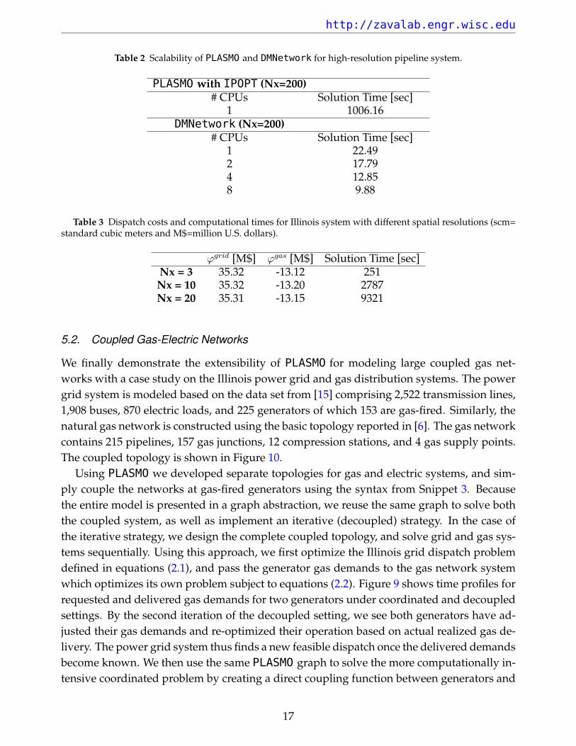
Table 2 shows the computational improvement of using high fidelity simulation to verifyour optimization problem. Using a high resolution of Nx =200 spatial mesh points and 24time points over a 24 hour horizon, the optimization problem takes over fifteen minutesto solve on an Intel(R) Core i7 CPU at 2.40GHz. The same optimization problem solvesin under three seconds using a coarse resolution of Nx =3 points per pipeline segment atthe same time resolution. For comparison, running a dynamic simulation using a Nx =200point discretization mesh in addition to a 96 point time resolution takes about 20 secondswith over a factor of 2 improvement using DMNetwork’s parallel simulation capabilities.

16



Table 2 Scalability of PLASMO and DMNetwork for high-resolution pipeline system.

PLASMO with IPOPT (Nx=200)# CPUs Solution Time [sec]

1 1006.16DMNetwork (Nx=200)

# CPUs Solution Time [sec]1 22.492 17.794 12.858 9.88

Table 3 Dispatch costs and computational times for Illinois system with different spatial resolutions (scm=standard cubic meters and M$=million U.S. dollars).

ϕgrid [M$] ϕgas [M$] Solution Time [sec]Nx = 3 35.32 -13.12 251

Nx = 10 35.32 -13.20 2787Nx = 20 35.31 -13.15 9321

5.2. Coupled Gas-Electric Networks

We finally demonstrate the extensibility of PLASMO for modeling large coupled gas net-works with a case study on the Illinois power grid and gas distribution systems. The powergrid system is modeled based on the data set from [15] comprising 2,522 transmission lines,1,908 buses, 870 electric loads, and 225 generators of which 153 are gas-fired. Similarly, thenatural gas network is constructed using the basic topology reported in [6]. The gas networkcontains 215 pipelines, 157 gas junctions, 12 compression stations, and 4 gas supply points.The coupled topology is shown in Figure 10.

Using PLASMO we developed separate topologies for gas and electric systems, and sim-ply couple the networks at gas-fired generators using the syntax from Snippet 3. Becausethe entire model is presented in a graph abstraction, we reuse the same graph to solve boththe coupled system, as well as implement an iterative (decoupled) strategy. In the case ofthe iterative strategy, we design the complete coupled topology, and solve grid and gas sys-tems sequentially. Using this approach, we first optimize the Illinois grid dispatch problemdefined in equations (2.1), and pass the generator gas demands to the gas network systemwhich optimizes its own problem subject to equations (2.2). Figure 9 shows time profiles forrequested and delivered gas demands for two generators under coordinated and decoupledsettings. By the second iteration of the decoupled setting, we see both generators have ad-justed their gas demands and re-optimized their operation based on actual realized gas de-livery. The power grid system thus finds a new feasible dispatch once the delivered demandsbecome known. We then use the same PLASMO graph to solve the more computationally in-tensive coordinated problem by creating a direct coupling function between generators and

17



demands. We warm-start the new nonlinear problem using the solution from the decoupledproblem. We have found this to be key to solve the coupled problem robustly. This is anotherbenefit of using PLASMO to generate warm-starting strategies. Figure 10 shows the spatialflow profiles throughout the gas system for the coupled and uncoupled problems at peaktime. Brighter links correspond to higher flows. We see that the coordinated setting (mid-dle) exhibits more homogeneous profiles compared to the decoupled setting (right). This isbecause coordination enables better balancing of pressures in the system, as discussed in [6].

0 5 10 15 20 250

1

2

3

4

Generator 1

Flow [SCM/h∗1

0−4

]

Iteration 1

0 5 10 15 20 250

1

2

3

4

Iteration 2

0 5 10 15 20 250

1

2

3

4

Coordinated

0 5 10 15 20 25Hour

0

1

2

3

4

5

6

7

8

Generator 2

Flow [SCM/h∗1

0−4

]

0 5 10 15 20 25Hour

0

1

2

3

4

5

6

7

8

0 5 10 15 20 25Hour

0

1

2

3

4

5

6

7

8

Fig. 9: Time profiles for requested and realized gas delivered for two Illinois power plants.

Fig. 10: Illinois grid and gas network (left), spatial flow profiles for coordinated dispatch(middle), and decoupled dispatch (right).

18



6. Conclusions

We have presented a computational framework that facilitates the construction, instantia-tion, and analysis of large-scale optimization and simulation applications of coupled energynetworks. The framework integrates the optimization modeling package PLASMO and thesimulation package DMNetwork (built around PETSc). We also describe how to embed thesetools within complex computational workflows using SWIFT, which is a tool that facilitatesparallel execution of multiple simulation runs and management of input and output data.We have found that the use of a common graph abstraction allows for seamless integrationof these tools. In addition, such an abstraction enables the creation of complex models incollaborative environments and facilitates the design of warm-starting and infrastructurecoordination strategies.

Acknowledgments

This material is based upon work supported by the U.S. Department of Energy, Office ofScience, under Contract No. DE-AC02-06CH11357.

7. References

[1] S. Abhyankar, B. Smith, H. Zhang, and A. Flueck. Using petsc to develop scalable appli-cations for next-generation power grid. In Proceedings of the first international workshopon High performance computing, networking and analytics for the power grid, pages 67–74.ACM, 2011.

[2] S. Balay, J. Brown, K. Buschelman, V. Eijkhout, W. D. Gropp, D. Kaushik, M. G. Knepley,L. C. McInnes, B. F. Smith, and H. Zhang. PETSc Web page. http://www.mcs.anl.gov/petsc, 2013.

[3] J. Bezanson, A. Edelman, S. Karpinski, and V. B. Shah. Julia: A fresh approach to nu-merical computing. arXiv, pages 1–37, 2015.

[4] R. G. Carter et al. Pipeline optimization: Dynamic programming after 30 years. In PSIGAnnual Meeting. Pipeline Simulation Interest Group, 1998.

[5] N. Chiang, C. G. Petra, and V. M. Zavala. Structured nonconvex optimization of large-scale energy systems using PIPS-NLP. In Proc. of the 18th Power Systems ComputationConference (PSCC), Wroclaw, Poland, 2014.

[6] N.-Y. Chiang and V. M. Zavala. Large-scale optimal control of interconnected naturalgas and electrical transmission systems. Applied Energy, 168:226–235, 2016.

[7] I. Dunning, J. Huchette, and M. Lubin. JuMP: A modeling language for mathematicaloptimization. arXiv:1508.01982 [math.OC], 2015.

19


http://www.mcs.anl.gov/petsc

http://www.mcs.anl.gov/petsc


[8] K. Kim, F. Yang, V. M. Zavala, and A. A. Chien. Data centers as dispatchable loads toharness stranded power. arXiv preprint arXiv:1606.00350, 2016.

[9] K. Kim and V. M. Zavala. Algorithmic innovations and software for the dual decompo-sition method applied to stochastic mixed-integer programs. Optimization Online, 2015.

[10] M. G. Knepley and D. A. Karpeev. Mesh algorithms for PDE with Sieve I: Mesh distribu-tion. Technical Report ANL/MCS-P1455-0907, Argonne National Laboratory, February2007. ftp://info.mcs.anl.gov/pub/tech_reports/reports/P1455.pdf.

[11] M. Shahidehpour, Y. Fu, and T. Wiedman. Impact of natural gas infrastructure on elec-tric power systems. Proceedings of the IEEE, 93(5):1042–1056, 2005.

[12] A. Wächter and L. T. Biegler. On the implementation of a primal-dual interior pointfilter line search algorithm for large-scale nonlinear programming. Mathematical Pro-gramming, 106:25–57, 2006.

[13] M. Wilde, M. Hategan, J. M. Wozniak, B. Clifford, D. S. Katz, and I. Foster. Swift: Alanguage for distributed parallel scripting. Parallel Computing, 37(9):633–652, 2011.

[14] V. M. Zavala. Stochastic optimal control model for natural gas networks. Computers &Chemical Engineering, 64:103–113, 2014.

[15] V. M. Zavala, A. Botterud, E. Constantinescu, and J. Wang. Computational and eco-nomic limitations of dispatch operations in the next-generation power grid. 2010 IEEEConference on Innovative Technologies for an Efficient and Reliable Electricity Supply, CITRES2010, pages 401–406, 2010.

[16] Y. Zhao, M. Hategan, B. Clifford, I. Foster, G. Von Laszewski, V. Nefedova, I. Raicu,T. Stef-Praun, and M. Wilde. Swift: Fast, reliable, loosely coupled parallel computation.In Services, 2007 IEEE Congress on, pages 199–206. IEEE, 2007.

[17] A. Zlotnik, M. Chertkov, and S. Backhaus. Optimal control of transient flow in naturalgas networks. In 2015 54th IEEE Conference on Decision and Control (CDC), pages 4563–4570. IEEE, 2015.

The submitted manuscript has been created by UChicago Argonne, LLC,Operator of Argonne National Laboratory (“Argonne”). Argonne, a U.S.Department of Energy Office of Science laboratory, is operated under Con-tract No. DE-AC02-06CH11357. The U.S. Government retains for itself, andothers acting on its behalf, a paid-up nonexclusive, irrevocable worldwidelicense in said article to reproduce, prepare derivative works, distributecopies to the public, and perform publicly and display publicly, by or onbehalf of the Government. The Department of Energy will provide publicaccess to these results of federally sponsored research in accordance withthe DOE Public Access Plan (http://energy.gov/downloads/doe-public-access-plan).

20


ftp://info.mcs.anl.gov/pub/tech_reports/reports/P1455.pdf

a graph-based computational framework for simulation … · a graph-based computational framework...

Documents