computational aspects of graph coloring and the quillen...

Computational Aspects of

Graph Coloring and the Quillen–Suslin Theorem

Troels Windfeldt

Department of Mathematical SciencesUniversity of Copenhagen

Denmark

Preface

This thesis is the result of research I have carried out during my time as aPhD student at the University of Copenhagen. It is based on four papers, theoverall topics of which are: Graph Coloring, The Quillen–Suslin Theorem, andSymmetric Ideals. The thesis is organized as follows.

Graph Coloring

Part 1 is, except for a few minor corrections, identical to the paper”Fibonacci Identities and Graph Colorings” (joint with C. Hillar, seepage 61), which has been accepted for publication in The FibonacciQuarterly. The paper introduces a simple idea that relates graphcoloring with certain integer sequences including the Fibonacci andLucas numbers. It demonstrates how one can produce identities in-volving these numbers by decomposing different classes of graphs indifferent ways. The treatment is by no means exhaustive, and thereshould be many ways to expand on the results presented in the paper.

Part 2 is an extended and improved version of the paper ”AlgebraicCharacterization of Uniquely Vertex Colorable Graphs” (joint withC. Hillar, see page 67), which has appeared in Journal of Combina-torial Theory, Series B. The paper deals with graph coloring from acomputational algebraic point of view. It collects a series of results inthe literature regarding graphs that are not k-colorable, and providesa refinement to uniquely k-colorable graphs. It also gives algorithmsfor testing (unique) vertex colorability. These algorithms are thenused to verify a counterexample to a conjecture of Xu concerninguniquely 3-colorable graphs without triangles.

i

The Quillen–Suslin Theorem

Part 3 is the manuscript ”Revisiting an Algorithm for the Quillen–SuslinTheorem”, which is still work in progress. It provides a new algo-rithm for the Quillen–Suslin Theorem in case of an infinite groundfield. The new algorithm follows the lines of an algorithm by Logarand Sturmfels, however, both theoretical and experimental evidencethat the new algorithm produces a much simpler output, is presented.This will hopefully facilitate its implementation in a computer alge-bra system.

Symmetric Ideals

Part 4 is an extended version of the short paper ”Minimal Generatorsfor Symmetric Ideals” (joint with C. Hillar, see page 82), which hasappeared in Proceedings of the American Mathematical Society. Thepaper settles a question regarding the minimal number of genera-tors for symmetric ideals in polynomial rings with infinitely manyindeterminates.

I would like to take this opportunity to thank my supervisor Henrik Schlichtkrullfor accepting me as his PhD student, for letting me pursue my own mathematicalinterests, and for supporting me all the way.

It has been a thrill working with my colleague and dear friend, Chris Hillar,who deserves a special thanks. I would also like to thank Niels Lauritzen andDavid Cox for many inspirational discussions on computational algebra.

Last, but not least, I thank my wife Gitte and daughter Emma for their contin-uous love and support.

Allerød,February 27, 2009, Troels Windfeldt.

ii

Contents

I Graph Coloring 1

1 Fibonacci Identities and Graph Colorings 2

1.1 Introduction . . . . . . . . . . . . . . . . . . . . . . . . . . . . . . 3

1.2 Identities . . . . . . . . . . . . . . . . . . . . . . . . . . . . . . . 6

1.3 Further Exploration . . . . . . . . . . . . . . . . . . . . . . . . . 8

2 Algebraic Characterization of UniquelyVertex Colorable Graphs 9

2.1 Introduction . . . . . . . . . . . . . . . . . . . . . . . . . . . . . . 10

2.2 Algebraic Preliminaries . . . . . . . . . . . . . . . . . . . . . . . 12

2.3 Characterization of Vertex Colorability . . . . . . . . . . . . . . . 14

2.4 Characterization of Unique Vertex Colorability . . . . . . . . . . 16

2.5 Algorithms for Testing (Unique) Vertex Colorability . . . . . . . 24

2.6 Verification of a Counterexample to Xu’s Conjecture . . . . . . . 27

2.7 Singular Libraries . . . . . . . . . . . . . . . . . . . . . . . . . 31

iii

II The Quillen–Suslin Theorem 37

3 Revisiting an Algorithm for the Quillen–Suslin Theorem 38

3.1 Introduction . . . . . . . . . . . . . . . . . . . . . . . . . . . . . . 39

3.2 Algorithm for the Unimodular Row Problem . . . . . . . . . . . 40

3.3 Complexity . . . . . . . . . . . . . . . . . . . . . . . . . . . . . . 44

3.4 Tricks and Drawbacks . . . . . . . . . . . . . . . . . . . . . . . . 47

III Symmetric Ideals 49

4 Minimal Generators for Symmetric Ideals 50

4.1 Introduction . . . . . . . . . . . . . . . . . . . . . . . . . . . . . . 51

4.2 Multisets and monomials . . . . . . . . . . . . . . . . . . . . . . 52

Bibliography 56

Summary in English 58

Summary in Danish 59

Papers to appear 60

Fibonacci Identities and Graph Colorings . . . . . . . . . . . . . . . . 61

Published papers 66

Algebraic Characterization of Uniquely Vertex Colorable Graphs . . . 67

Minimal Generators for Symmetric Ideals . . . . . . . . . . . . . . . . 82

iv

I

Graph Coloring

1

Part 1

Fibonacci Identities andGraph Colorings

We generalize both the Fibonacci and Lucas numbers to the context of graphcolorings, and prove some identities involving these numbers. As a corollary weobtain new proofs of some known identities involving Fibonacci numbers suchas

Fr+s+t = Fr+1Fs+1Ft+1 + FrFsFt − Fr−1Fs−1Ft−1.

2

1.1 Introduction

In graph theory, it is natural to study vertex colorings, and more specifically,those colorings in which adjacent vertices have different colors. In this case, thenumber of such colorings of a graph G is encoded by the chromatic polynomial ofG. This object can be computed using the method of “deletion and contraction”,which involves the recursive combination of chromatic polynomials for smallergraphs. The purpose of this note is to show how the Fibonacci and Lucasnumbers (and other integer recurrences) arise naturally in this context, andin particular, how identities among these numbers can be generated from thedifferent choices for decomposing a graph into smaller pieces.

We first introduce some notation. Let G be a undirected graph (possibly con-taining loops and multiple edges) with vertices V = {1, . . . , n} and edges E.Given nonnegative integers k and `, a (k, `)-coloring of G is a map

ϕ : V → {c1, . . . , ck+`},in which {c1, . . . , ck+`} is a fixed set of k+` “colors”. The map ϕ is called properif whenever i is adjacent to j and ϕ(i), ϕ(j) ∈ {c1, . . . , ck}, we have ϕ(i) 6= ϕ(j).Otherwise, we say that the map ϕ is improper. In somewhat looser terminology,one can think of {ck+1, . . . , ck+`} as coloring “wildcards”.

Let χG(x, y) be a function such that χG(k, `) is the number of proper (k, `)-colorings of G. This object was introduced by the authors of [DPT03] andcan be given as a polynomial in x and y (see Lemma 1.1.1). It simultane-ously generalizes the chromatic, independence, and matching polynomials of G.For instance, χG(x, 0) is the usual chromatic polynomial while χG(x, 1) is theindependence polynomial for G (see [DPT03] for more details).

We next state a simple rule that enables one to calculate the polynomial χG(x, y)recursively. In what follows, G\e denotes the graph obtained by removing theedge e from G, and for a subgraph H of G, the graph G\H is gotten fromG by removing H and all the edges of G that are adjacent to vertices of H.Additionally, the contraction of an edge e in G is the graph G/e obtained byremoving e and identifying as equal the two vertices sharing this edge.

Lemma 1.1.1. Let e be an edge in G, and let v be the vertex to which e contractsin G/e. Then,

χG(x, y) = χG\e(x, y)− χG/e(x, y) + y · χ(G/e)\v(x, y). (1.1.1)

3

Proof. The number of proper (k, `)-colorings of G\e which have distinct colorsfor the vertices sharing edge e is given by χG\e(k, `)−χG/e(k, `); these coloringsare also proper for G. The remaining proper (k, `)-colorings of G are preciselythose for which the vertices sharing edge e have the same color. This color mustbe one of the wildcards {ck+1, . . . , ck+`}, and so the number of remaining proper(k, `)-colorings of G is counted by ` · χ(G/e)\v(k, `).

With such a recurrence, we need to specify initial conditions. When G simplyconsists of one vertex and has no edges, we have χG(x, y) = x+ y, and when Gis the empty graph, we set χG(x, y) = 1 (consider G with one edge joining twovertices in (1.1.1)). Moreover, χ is multiplicative on disconnected components.This allows us to compute χG for any graph recursively.

In the special case when k = 1, there is also a way to calculate χG(1, y) byremoving vertices from G. Define the link of a vertex v to be the subgraphlink(v) of G consisting of v, the edges touching v, and the vertices sharing oneof these edges with v. Also if u and v are joined by an edge e, we define link(e)to be link(u) ∪ link(v) in G, and also we set deg(e) to be deg(u) + deg(v) − 2.We then have the following rules.

Lemma 1.1.2. Let v be any vertex of G, and let e be any edge. Then,

χG(1, y) = y · χG\v(1, y) + ydeg(v) · χG\link(v)(1, y), (1.1.2)

χG(1, y) = χG\e(1, y)− ydeg(e) · χG\link(e)(1, y). (1.1.3)

Proof. The number of proper (1, `)-colorings of G with vertex v colored with awildcard is ` · χG\v(1, `). Moreover, in any proper coloring of G with v coloredc1, each vertex among the deg(v) ones adjacent to v can only be one of the `wildcards. This explains the first equality in the lemma.

Let v be the vertex to which e contracts in G/e. From equation (1.1.2), we have

χG/e(1, y) = y · χ(G/e)\v(1, y) + ydeg(v) · χ(G/e)\link(v)(1, y).

Subtracting this equation from (1.1.1) with x = 1, and noting that deg(e) =deg(v) and G\link(e) = (G/e)\link(v), we arrive at the second equality in thelemma.

Let Pn be the path graph on n vertices and let Cn be the cycle graph, also onn vertices (C1 is a vertex with a loop attached while C2 is two vertices joined

4

by two edges). Fixing nonnegative integers k and ` not both zero, we define thefollowing sequences of numbers (n ≥ 1):

an = χPn(k, `),

bn = χCn(k, `).

(1.1.4)

As we shall see, these numbers are natural generalizations of both the Fibonacciand Lucas numbers to the context of graph colorings. The following lemma usesgraph decomposition to give simple recurrences for these sequences.

Lemma 1.1.3. The sequences an and bn satisfy the following linear recurrenceswith initial conditions:

a1 = k + `, a2 = (k + `)2 − k, an = (k + `− 1)an−1 + àn−2; (1.1.5)

b1 = `, b2 = (k + `)2 − k, b3 = a3 − b2 + à1, (1.1.6)

bn = (k + `− 2)bn−1 + (k + 2`− 1)bn−2 + `bn−3. (1.1.7)

Moreover, the sequence bn satisfies a shorter recurrence if and only if k = 0,k = 1, or ` = 0. When k = 0, this recurrence is given by bn = `bn−1, and whenk = 1, it is

bn = `bn−1 + `bn−2. (1.1.8)

Proof. The first recurrence follows from deleting an outer edge of the path graphPn and using Lemma 1.1.1. To verify the second one, we first use Lemma 1.1.1(picking any edge in Cn) to give

bn = an − bn−1 + àn−2. (1.1.9)

Let cn = bn+bn−1 = an+àn−2 and notice that cn satisfies the same recurrenceas an; namely,

cn = an + àn−2

= (k + `− 1)an−1 + àn−2 + ` ((k + `− 1)an−3 + àn−4)= (k + `− 1)(an−1 + àn−3) + `(an−2 + àn−4)= (k + `− 1)cn−1 + `cn−2.

(1.1.10)

It follows that bn satisfies the third order recurrence given in the statement ofthe lemma. Additionally, the initial conditions for both sequences an and bnare easily worked out to be the ones shown.

5

Finally, suppose that the sequence bn satisfies a shorter recurrence,

bn + rbn−1 + sbn−2 = 0,

and let

B =

b3 b2 b1b4 b3 b2b5 b4 b3

.

Since the nonzero vector [1, r, s]T is in the kernel of B, we must have that

0 = det(B) = −k2(k − 1)`((k + `− 1)2 + 4`).

It follows that for bn to satisfy a smaller recurrence, we must have k = 0, k = 1,or ` = 0. It is clear that when k = 0, we have bn = `n = `bn−1. When k = 1,we can use Lemma 1.1.2 to see that

bn+1 = `(an + `an−2),

and combining this with (1.1.9) gives the recurrence stated in the lemma.

When k = 1 and ` = 1, the recurrences given by Lemma 1.1.3 when appliedto the families of path graphs and cycle graphs are the Fibonacci and Lucasnumbers, respectively. This observation is well-known (see [Kos01, Examples4.1 and 5.3]) and was brought to our attention by Cox [Cox]:

χPn(1, 1) = Fn+2 and χCn

(1, 1) = Ln. (1.1.11)

Moreover, when k = 2 and ` = 1, the recurrence given by Lemma 1.1.3 whenapplied to the family of path graphs is the one associated to the Pell numbers:

χPn(2, 1) = Qn+1,

where Q0 = 1, Q1 = 1, and Qn = 2Qn−1 +Qn−2.

1.2 Identities

In this section, we derive some identities involving the generalized Fibonacci andLucas numbers an and bn using the graph coloring interpretation found here.

6

In what follows, we fix k = 1. In this case, the an and bn satisfy the followingrecurrences:

an = àn−1 + àn−2 and bn = `bn−1 + `bn−2.

Theorem 1.2.1. The following identities hold:

bn = àn−1 + `2an−3, (1.2.1)

bn = an − `2an−4, (1.2.2)

ar+s = àras−1 + `2ar−1as−2, (1.2.3)

ar+s = aras − `2ar−2as−2, (1.2.4)

ar+s+t+1 = àrasat + `3ar−1as−1at−1 − `4ar−2as−2at−2. (1.2.5)

Proof. All of the above identities follow from Lemma 1.1.2 when applied todifferent graphs (with certain choices of vertices and edges). To see the first twoequations, consider the cycle graph Cn and pick any vertex and any edge. Tosee the next two equations, consider the path graph Pr+s with v = r + 1 ande = {r, r + 1}.

r vertices t vertices

s vertices

ev

In order to prove the final equation in the statement of the theorem, considerthe graph G in the above figure. It follows from Lemma 1.1.2 that

àr+sat + `3ar−1as−1at−1 = ar+s+t+1 − `4ar−2as−2at−1.

7

Rearranging the terms and applying (1.2.4), we see that

ar+s+t+1 = àr+sat + `3ar−1as−1at−1 + `4ar−2as−2at−1

= `(aras − `2ar−2as−2)at + `3ar−1as−1at−1 + `4ar−2as−2at−1

= àrasat − `3ar−2as−2(àt−1 + àt−2)

+ `3ar−1as−1at−1 + `4ar−2as−2at−1

= àrasat + `3ar−1as−1at−1 − `4ar−2as−2at−2.

This completes the proof of the theorem.

Corollary 1.2.2. The following identities hold:

Ln = Fn+1 + Fn−1,

Ln = Fn+2 − Fn−2,

Fr+s = Fr+1Fs + FrFs−1,

Fr+s = Fr+1Fs+1 − Fr−1Fs−1,


Proof. The identities follow from the corresponding ones in Theorem 1.2.1 with` = 1 by making suitable shifts of the indices and using (1.1.11).

1.3 Further Exploration

In this note, we have produced recurrences and identities by decomposing differ-ent classes of graphs in different ways. Our treatment is by no means exhaustive,and there should be many ways to expand on what we have done here. For in-stance, is there a graph coloring proof of Cassini’s identity?

8

Part 2

Algebraic Charac-terization of UniquelyVertex Colorable Graphs

The study of graph vertex colorability from an algebraic perspective has intro-duced novel techniques and algorithms into the field. For instance, it is knownthat k-colorability of a graph G is equivalent to the condition 1 ∈ IG,k fora certain ideal IG,k ⊆ k[x1, . . . , xn]. In this paper, we extend this result byproving a general decomposition result for IG,k. This will allow us to give analgebraic characterization of uniquely k-colorable graphs. Our results also givealgorithms for testing (unique) vertex colorability. As an application, we verifya counterexample to a conjecture of Xu concerning uniquely 3-colorable graphswithout triangles.

9

2.1 Introduction

Let G be a simple, undirected graph with vertices V = {1, . . . , n} and edges E.Fix a positive integer k ≤ n, and let Ck = {c1, . . . , ck} be a k-element set. Eachelement of Ck is called a color. A (vertex) k-coloring of G is a map γ : V → Ck.We say that a k-coloring γ is proper if adjacent vertices receive different colors;otherwise γ is improper. The graph G is said to be k-colorable if there exists aproper k-coloring of G.

Let k be an algebraically closed field of characteristic not dividing k. We willbe interested in the following ideals of the polynomial ring k[x1, . . . , xn] over kin indeterminates x1, . . . , xn:

In,k =⟨xki − 1 : i ∈ V

⟩, (2.1.1)

and

IG,k = In,k +⟨xk−1i + xk−2

i xj + · · ·+ xixk−2j + xk−1

j : {i, j} ∈ E⟩. (2.1.2)

One should think of (the zeros of) In,k and IG,k as representing k-colorings andproper k-colorings of the graph G, respectively (see Section 2.3). The idea ofusing roots of unity and ideal theory to study graph coloring problems seemsto originate in Bayer’s thesis [Bay82], although it has appeared in many otherplaces. The following theorem establishes an important connection between thegraph ideal IG,k and the number of proper k-colorings of G.

Theorem 2.1.1. The vector space dimension of k[x1, . . . , xn]/IG,k over k equalsthe number of proper k-colorings of G.

This key theorem seems to have gone unnoticed in the literature. We present aproof of it in Section 2.3.

The ideals In,k and IG,k are also important because they, together with thegraph polynomial of G given by

fG =∏

{i,j}∈E,i<j

(xi − xj),

allow for an algebraic formulation of k-colorability. The following theorem col-lects some of the results in the series of works [AT92, Bay82, dL95].

10

Theorem 2.1.2. The following statements are equivalent:

(1) The graph G is not k-colorable.(2) The vector space dimension of k[x1, . . . , xn]/IG,k over k is zero.(3) The constant polynomial 1 belongs to the graph ideal IG,k.(4) The graph polynomial fG belongs to the ideal In,k.

The equivalence between (1) and (2) follows from Theorem 2.1.1. The equiva-lence between (1) and (3) is due to Bayer [Bay82, pp. 109–112] (see also Chapter2.7 of [AL94]). Alon and Tarsi [AT92] proved that (1) and (4) are equivalent,but also de Loera [dL95] have proved this using Grobner basis methods. Wegive a self-contained and simplified proof of Theorem 2.1.2 in Section 2.3, inpart to collect the many facts we need here.

We say that a graph is uniquely k-colorable if there is a unique proper k-coloringup to permutation of the colors. In this case, partitions of the vertices into sub-sets having the same color are the same for each of the k! proper k-coloringsof G. A natural refinement of Theorem 2.1.2 would be an algebraic characteri-zation of when a k-colorable graph is uniquely k-colorable. We provide such acharacterization.

Theorem 2.1.3. The following statements are equivalent:

(1) The graph G is uniquely k-colorable.(2) The vector space dimension of k[x1, . . . , xn]/IG,k over k is k!.(3) The polynomials g1, . . . , gn belong to the graph ideal IG,k.(4) The graph polynomial fG belongs to the ideal In,k : 〈g1, . . . , gn〉.

The polynomials g1, . . . , gn in (3) and (4) are given by (2.4.3) in Lemma 2.4.4for some proper k-coloring of G, and some complete set of representatives of thecolor classes.

Remark 2.1.4. It is important to point out that one need not have a properk-coloring of a given graph G (nor the polynomials g1, . . . , gn) in order to testif G is uniquely k-colorable using (2) of Theorem 2.1.3. This is only necessarywhen using (3) or (4).

11

The organization of this paper is as follows. In Section 2.2 we discuss some ofthe algebraic tools that will go into the proofs of our main results. Section 2.3is devoted to proofs of Theorems 2.1.1 and 2.1.2. In Section 2.4 we develop theconcept of coloring ideals, and use it to prove Theorem 2.1.3. Theorems 2.1.2and 2.1.3 give algorithms for testing k-colorability and unique k-colorability ofgraphs, and we discuss an implementation of them in Section 2.5. These al-gorithms we then use in Section 2.6 to verify a counterexample [AMS01] to aconjecture [Xu90] by Xu concerning uniquely 3-colorable graphs without tri-angles. In this section we also discuss the tractability of our algorithms. Wehope that they might be used to perform experiments for raising and settlingproblems in the theory of (unique) vertex colorability.

2.2 Algebraic Preliminaries

We briefly review the basic concepts of commutative algebra that will be usefulfor us here. We refer to [AL94, CLO07, CLO05, KR00] for more details.

Let I be an ideal of k[x1, . . . , xn]. The variety V (I) of I is the set of points inkn that are zeros of all the polynomials in I. Conversely, the vanishing idealI(V ) of a set V ⊆ kn is the ideal of those polynomials vanishing on all of V .These two definitions are related by way of V (I(V )) = V and I(V (I)) =

√I

(the latter equality is known as Hilbert’s Nullstellensatz), in which√I = {f : fn ∈ I for some n}

is the radical of I. The ideal I is said to be a radical ideal if it is equal to itsradical. The ideal I is said to be zero-dimensional if V (I) is finite.

Many arguments in commutative algebra and algebraic geometry are simplifiedwhen restricted to radical, zero-dimensional ideals (resp. multiplicity-free, finitevarieties), and those found in this paper are not exceptions. The following twofacts are useful in this regard.

Lemma 2.2.1. Let I ⊆ k[x1, . . . , xn] be a zero-dimensional ideal. If I containsa non-zero univariate square-free polynomial in each indeterminate then I is aradical ideal.

Proof. See [KR00, p. 250, Proposition 3.7.15].

12

Lemma 2.2.2. Let I ⊆ k[x1, . . . , xn] be a zero-dimensional ideal. The vectorspace dimension of k[x1, . . . , xn]/I over k is greater than or equal to the numberof points in the variety V (I). Furthermore, equality occurs if and only if I is aradical ideal.

Proof. See [CLO05, pp. 43–44, Theorem 2.10].

A term order ≺ for the monomials of k[x1, . . . , xn] is a well-ordering which ismultiplicative (u ≺ v =⇒ wu ≺ wv for monomials u, v, w) and for which theconstant monomial 1 is smallest. The leading monomial lm≺(f) of a polynomialf ∈ k[x1, . . . , xn] is the largest monomial in f with respect to ≺. The standardmonomials of I are those monomials which are not the leading monomial of anypolynomial in I.

Lemma 2.2.3. Let I ⊆ k[x1, . . . , xn] be an ideal, and let ≺ be a term order.The vector space k[x1, . . . , xn]/I over k is isomorphic to the vector space overk spanned by the standard monomials of I.

Proof. See [CLO07, p. 232, Proposition 4].

A finite subset G of an ideal I is said to be a Grobner basis for I (with respectto the term order ≺) if the leading ideal,

lm≺(I) = 〈lm≺(f) : f ∈ I〉 ,

is generated by the leading monomials of elements of G. It is called minimal if noleading monomial of g ∈ G divides any other leading monomial of polynomialsin G. Many of the properties of I and V (I) can be calculated by finding aGrobner basis for I, and such generating sets are fundamental for computation(including the algorithms presented in Section 2.5).

Finally, a useful operation on two ideals I and J is the construction of the colonideal I : J = {f ∈ k[x1, . . . , xn] : fJ ⊆ I}. If V and W are two varieties, thenthe colon ideal

I(V ) : I(W ) = I(V \W ) (2.2.1)

corresponds to a set difference. We conclude this section by noticing that

K ⊆ I : J ⇐⇒ J ⊆ I : K (2.2.2)

13

for ideals I, J , and K. The reader is referred to [CLO07, pp. 194–196] forproofs of these facts.

2.3 Characterization of Vertex Colorability

In what follows, the set Ck = {c1, . . . , ck} of colors will be the set of kth rootsof unity, and we shall freely speak of points in kn with all coordinates in Ck ask-colorings of G. In this case, a point γ = (γ1, . . . , γn) ∈ kn corresponds to acoloring of vertex i with color γi for i = 1, . . . , n. Furthermore, let Γn,k ⊆ knbe the set of all k-colorings of G, and let ΓG,k ⊆ kn be the set of all properk-colorings of G.

The next result will prove useful in simplifying many of the proofs in this sectionand the next one.

Lemma 2.3.1. In,k and IG,k are zero-dimensional radical ideals.

Proof. Equations (2.1.1) and (2.1.2) show that V (IG,k) ⊆ V (In,k) = Γn,k, whichmeans that In,k and IG,k are zero-dimensional.

If we let fi = xki − 1 then f ′i = kxk−1i 6= 0, since the characteristic of k does not

divide k. This shows that gcd(fi, f ′i) = 1 and so fi is square-free. It now followsfrom Lemma 2.2.1 that In,k is a radical ideal. The same argument works forIG,k, since In,k ⊆ IG,k.

Lemma 2.3.2. In,k and IG,k are the vanishing ideals of the set of all k-coloringsof G and the set of all proper k-colorings of G, respectively.

Proof. From Equation (2.1.1) it is clear that V (In,k) = Γn,k. Hilbert’s Nullstel-lensatz then tells us that In,k = I(Γn,k), since In,k is a radical ideal.

From Equation (2.1.2) it is not quite so obvious that V (IG,k) = ΓG,k. To seethis, first notice that V (IG,k) ⊆ V (In,k) = Γn,k. Next, let

hk−1{i,j} = xk−1

i + xk−2i xj + · · ·+ xix

k−2j + xk−1

j ,

and let γ = (γ1, . . . , γn) ∈ Γn,k be any k-coloring of G. If γ is improper thereexists an edge {i, j} ∈ E for which γi = γj . Then hk−1

{i,j}(γ) = kγk−1i 6= 0, since

14

the characteristic of k does not divide k. This shows that V (IG,k) ⊆ ΓG,k. Toget the reverse direction, notice that

(γi − γj)hk−1{i,j}(γ) = γki − γkj = 1− 1 = 0.

Hence, if γ is proper, we have hk−1{i,j}(γ) = 0 for all {i, j} ∈ E. This shows that

ΓG,k ⊆ V (IG,k). As before, Hilbert’s Nullstellensatz tells us that IG,k = I(ΓG,k),since IG,k is also a radical ideal.

We are now in a position to prove our first main theorem.

Proof of Theorem 2.1.1. According to Lemma 2.2.2, the vector space dimensionof k[x1, . . . , xn]/IG,k over k equals the number of points in the variety V (IG,k),since IG,k is a radical ideal. The result now follows since V (IG,k) is the set ofall proper k-colorings of G as a result of Lemma 2.3.2.

The next result describes a simple relationship between the ideals In,k and IG,k,and the graph polynomial fG.

Lemma 2.3.3. In,k : 〈fG〉 = IG,k.

Proof. The first step is to note that 〈fG〉 is a radical ideal. This follows from[CLO07, p. 180, Proposition 9], since fG is square-free. Hilbert’s Nullstellensatzthen implies that

〈fG〉 = I(V (〈fG〉)). (2.3.1)

Next, let γ = (γ1, . . . , γn) ∈ Γn,k be any k-coloring of G. It is clear thatfG(γ) = 0 if and only if γ is improper. Hence, we see that

Γn,k\V (〈fG〉) = ΓG,k. (2.3.2)

The result now follows from the string of equations:

In,k : 〈fG〉 = I(Γn,k) : 〈fG〉 by Lemma 2.3.2= I(Γn,k) : I(V (〈fG〉)) by Equation (2.3.1)= I(Γn,k\V (〈fG〉)) by Equation (2.2.1)= I(ΓG,k) by Equation (2.3.2)= IG,k by Lemma 2.3.2.

15

We now prove Theorem 2.1.2. We feel that it is the most efficient proof of thisresult.

Proof of Theorem 2.1.2.

(1)⇐⇒ (2): The graph G is not k-colorable if and only if the number of properk-colorings of G is zero. Theorem 2.1.1 shows that this happens if andonly if the vector space dimension of k[x1, . . . , xn]/IG,k over k is zero.

(2)⇐⇒ (3): The vector space dimension of k[x1, . . . , xn]/IG,k is zero if andonly if IG,k = k[x1, . . . , xn], which is the case if and only if the constantpolynomial 1 belongs to the graph ideal IG,k.

(3)⇐⇒ (4): Recall that In,k : 〈fG〉 = IG,k according to Lemma 2.3.3, andnotice that In,k : 〈1〉 = In,k by definition. The equivalence now followsfrom (2.2.2) with I = In,k, J = 〈fG〉, and K = 〈1〉.

2.4 Characterization of UniqueVertex Colorability

Let γ be any k-coloring of G. Any k-coloring of G that arises from γ by apermutation of the colors is said to be essentially identical to γ. Let ΓG,γ ⊆ knbe the set of all k-colorings of G that are essentially identical to γ. The vanishingideal I(ΓG,γ) is said to be the coloring ideal IG,γ associated to γ.

Our first result about coloring ideals is the following simple lemma, which is ananalogue of Lemma 2.3.1.

Lemma 2.4.1. IG,γ is a zero-dimensional radical ideal.

Proof. The variety V (IG,γ) = ΓG,γ is finite since there is only a finite numberof permutations of the k colors. Any vanishing ideal is a radical ideal.

16

In fact, it is not difficult to determine the exact number of k-colorings of G thatare essentially identical to γ. If γ uses ` ≤ k of the available colors, then thenumber of such k-colorings is

|ΓG,γ | =(k

`

)`!. (2.4.1)

The next result is similar to Lemma 2.3.3, but instead it decomposes the graphideal IG,k in terms of coloring ideals.

Lemma 2.4.2.⋂γ∈ΓG,k

IG,γ = IG,k.

Proof. If γ ∈ ΓG,k is a proper k-colorings of G, then all essentially identicalk-colorings of G are proper too. Hence, we see that

⋃

γ∈ΓG,k

ΓG,γ = ΓG,k. (2.4.2)

The result now follows from the string of equations:⋂

γ∈ΓG,k

IG,γ =⋂

γ∈ΓG,k

I(ΓG,γ) by definition

= I(ΓG,k) by Equation (2.4.2)= IG,k by Lemma 2.3.2.

For a subset U ⊆ V of vertices and a positive integer d, let hdU be the sum ofall monomials of degree d in the indeterminates {x` : ` ∈ U}. Also, let h0

U = 1.The polynomial hdU is obviously homogeneous of degree d, and symmetric in theindeterminates {x` : ` ∈ U}.

The following lemma is a very important ingredient in the proof of Lemma 2.4.4.

Lemma 2.4.3. If {i, j} ⊆ U , then

(xi − xj)hdU = hd+1U\{j} − hd+1

U\{i},

for all non-negative integers d.

17

Proof. The first step is to note that the polynomial xihdU +hd+1U\{i} is symmetric

in the indeterminates {x` : ` ∈ U}. This follows from the polynomial identity

hd+1U − hd+1

U\{i} = xihdU ,

and the fact that hd+1U is symmetric in the indeterminates {x` : ` ∈ U}. Let σ

be the transposition (i j), and note that

xihdU + hd+1

U\{i} = σ(xih

dU + hd+1

U\{i}

)= xjh

dU + hd+1

U\{j}.

This concludes the proof.

The next result is an important technical lemma that describes special sets ofgenerators for coloring ideals.

Lemma 2.4.4. Let γ be any k-coloring of G, and let {v1, . . . , v`} ⊆ V be anycomplete set of representatives of the color classes in which γ partitions V . Forany vertex i ∈ V , denote by v(i) the representative having the same color as i.The coloring ideal IG,γ associated to γ is generated by the polynomials g1, . . . , gndefined by

gi =

xkv1 − 1 if i = v1,

hk+1−j{v1,...,vj} if i = vj for any j > 1,

xi − xv(i) otherwise.

(2.4.3)

Moreover, the set G = {g1, . . . , gn} of polynomials form a minimal Grobner basisfor the ideal IG,γ with respect to any term order ≺ satisfying xv1 ≺ · · · ≺ xv`

,and xv(i) ≺ xi for all vertices i ∈ V \ {v1, . . . , v`}.

Proof. We begin by proving that I = 〈g1, . . . , gn〉 vanishes on all the k-coloringsof G that are essentially identical to γ. Suppose δ = (δ1, . . . , δn) ∈ ΓG,γ is sucha k-coloring of G. First of all, it is obvious that

gv1(δ) = δkv1 − 1 = 1− 1 = 0.

We will prove that also gv2 , . . . , gv`vanish on δ by establishing the following

stronger statement using induction on |U |:

hk+1−|U |U (δ) = 0 for all subsets U ⊆ {v1, . . . , v`} with |U | > 1. (∗)

18

In the case |U | = 2, we have U = {u1, u2}. It is easily verified that

(δu1 − δu2)hk−1U (δ) = δku1

− δku2= 1− 1 = 0.

Since U ⊆ {v1, . . . , v`}, we have δu1 6= δu2 and so hk−1U (δ) = 0. This shows

that (∗) holds for all subsets U ⊆ {v1, . . . , v`} with |U | = 2. In the generalcase, we have {u1, u2} ⊂ U . It now follows from Lemma 2.4.3 and the inductionhypothesis, that

(δu1 − δu2)hk+1−|U |U (δ) = h

k+1−|U\{u2}|U\{u2} (δ)− hk+1−|U\{u1}|

U\{u1} (δ) = 0.

As before, we have hk+1−|U |U (δ) = 0, and this completes the proof of (∗). Finally

we need to show that the remaining generators of I also vanish on δ. Thisfollows immediately from that fact that

gi(δ) = δi − δv(i) = 0,

since δ partitions V into the same color classes as γ does, and v(i) is the repre-sentative having the same color as i ∈ V . We have therefore now proved that Ivanishes on all the k-colorings of G that are essentially identical to γ, that is,I ⊆ IG,γ . It now follows immediately that

V (I) ⊇ V (IG,γ). (2.4.4)

We continue the proof by showing that the ideals I and IG,γ give rise to thesame variety. Let ≺ be any term order satisfying xv1 ≺ · · · ≺ xv`

, and xv(i) ≺ xifor all vertices i ∈ V \ {v1, . . . , v`}. By inspecting (2.4.3) we see that the leadingmonomial of gi is given by

lm≺(gi) =

{xk+1−ji if i = vj for any j ≥ 1,xi otherwise.

The leading monomials of g1, . . . , gn are therefore pairwise relatively prime. Itfollows that the set G = {g1, . . . , gn} of polynomials form a minimal Grobnerbasis for the ideal I with respect to the term order ≺ (see [AL94, Theorem 1.7.4and Lemma 3.3.1]). Furthermore, for each i = 1, . . . , n there is a g ∈ G withleading monomial that is a power of xi. This implies that V (I) is finite, that is,I is a zero-dimensional ideal (see [AL94, Theorem 2.2.7]).

The set of standard monomials of I with respect to ≺ is readily seen to be theset

S ={xαjvj

: αj < k + 1− j for j = 1, . . . , `}. (2.4.5)

19

The vector space k[x1, . . . , xn]/I is, according to Lemma 2.2.3, isomorphic tothe vector space over k spanned by S, that is,

k[x1, . . . , xn]/I ' spank S. (2.4.6)

We may now write

k(k − 1) · · · (k + 1− `) = |ΓG,γ | by Equation (2.4.1)= |V (IG,γ)| by definition≤ |V (I)| by (2.4.4)≤ dim k[x1, . . . , xn]/I by Lemma 2.2.2= dim spank S by (2.4.6)= k(k − 1) · · · (k + 1− `) by (2.4.5).

Hence, equality holds throughout. In particular, we have |V (IG,γ)| = |V (I)|which, together with (2.4.4), shows that the ideals I and IG,γ give rise to thesame variety, that is,

V (I) = V (IG,γ). (2.4.7)

Furthermore, we also see that the vector space dimension of k[x1, . . . , xn]/I overk equals the number of points in the variety V (I), and so I is a radical idealaccording to Lemma 2.2.2. Since IG,γ , by Lemma 2.4.1, is also a radical ideal,Equation (2.4.7) and Hilbert’s Nullstellensatz finally imply that I = IG,γ , whichthen concludes the proof.

We present three examples that demonstrate Lemma 2.4.4.

Example 2.4.5. Let G be the complete graph on n vertices, and let γ be anyproper n-coloring of G. The color classes each consist of a single vertex, and sowe may choose the representative vj = j for j = 1, . . . , n. The coloring idealassociated to γ is therefore given by

IG,γ =⟨xn1 − 1, xn−1

1 + xn−21 x2 + · · ·+ x1x

n−22 + xn−1

2 , . . . , x1 + · · ·+ xn⟩.

Example 2.4.6. Let G be the graph in Figure 2.1, and let γ be the indicated3-coloring of G. We may choose the set v1 = 12, v2 = 11, and v3 = 10 asrepresentatives of the color classes in which γ partitions V . The coloring ideal

20

Figure 2.1: A uniquely 3-colorable graph without triangles [CC93].

associated to γ is therefore given by

IG,γ = 〈x312 − 1, x7 − x12, x4 − x12, x3 − x12,

x211 + x11x12 + x2

12, x9 − x11, x6 − x11, x2 − x11,

x10 + x11 + x12, x8 − x10, x5 − x10, x1 − x10〉.

The generators form a minimal Grobner basis for the ideal IG,γ with respect toany term ordering with e.g. x12 ≺ · · · ≺ x1. The leading term (with respect tosuch a term order) of each polynomial is underlined. Notice that the leadingterms of the polynomials in each line correspond to the different color classes ofthis coloring of G.

The third example also demonstrates Lemma 2.4.2.

Example 2.4.7. Let G = ({1, 2, 3}, {{1, 2}, {2, 3}}) be the path graph on threevertices. There are essentially two proper 3-colorings of G: the one wherevertices 1 and 3 receive the same color, and the one where all the verticesreceive different colors. If we denote by γ1 the former, and by γ2 the latter, itfollows from Lemma 2.4.4 that

IG,γ1 =⟨x3

1 − 1, x21 + x1x2 + x2

2, x3 − x1

⟩,

IG,γ2 =⟨x3

1 − 1, x21 + x1x2 + x2

2, x1 + x2 + x3

⟩.

Lemma 2.4.2 predicts that the intersection IG,γ1 ∩ IG,γ2 is equal to the graph

21

ideal

IG,3 =⟨x3

1 − 1, x32 − 1, x3

3 − 1, x21 + x1x2 + x2

2, x22 + x2x3 + x2

3

⟩.

It is possible to verify this using the computer algebra system Singular asshown by the following piece of code. For more information about Singularand the libraries graph.lib and ideals.lib that are being used, the reader isreferred to Section 2.7.

> int n = 3;> ring R = 0, x(1..n), lp;> list G = pathgraph(n);> list gamma1 = 3, list(intvec(1,3), 2);> ideal I1 = I(G, gamma1);> I1;I1[1]=x(1)^3-1I1[2]=x(1)^2+x(1)*x(2)+x(2)^2I1[3]=-x(1)+x(3)> list gamma2 = 3, list(1, 2, 3);> ideal I2 = I(G, gamma2);> I2;I2[1]=x(1)^3-1I2[2]=x(1)^2+x(1)*x(2)+x(2)^2I2[3]=x(1)+x(2)+x(3)> groebner(intersect(I1, I2));_[1]=x(3)^3-1_[2]=x(2)^2+x(2)*x(3)+x(3)^2_[3]=x(1)^2+x(1)*x(2)-x(2)*x(3)-x(3)^2> groebner(I(G, 3));_[1]=x(3)^3-1_[2]=x(2)^2+x(2)*x(3)+x(3)^2_[3]=x(1)^2+x(1)*x(2)-x(2)*x(3)-x(3)^2

The two Grobner basis computations yield the same result, which means thetwo ideals IG,γ1 ∩ IG,γ2 and IG,3 are the same.

We are now ready to prove our characterization of uniquely k-colorable graphs.Before we begin though, we need the following elementary observation.

22

Lemma 2.4.8. If a graph G is k-colorable, then there exists a proper k-coloringof G that uses all k colors.

Proof. Suppose γ is a proper k-coloring of a graph G. If γ uses all k colors, thenwe are done. Now suppose γ uses only ` < k colors. Then ` < n so there mustbe two vertices with the same color. Give one of these one of the unused colors.The resulting k-coloring of G is still proper but uses `+ 1 colors. Continue thisway until a proper k-coloring of G that uses all k colors is reached.

Proof of Theorem 2.1.3.

(1)⇐⇒ (2): Suppose the graph G is uniquely k-colorable. By Lemma 2.4.8there exists a proper k-coloring of G that uses all k colors. Since Gis uniquely k-colorable, all other proper k-colorings of G are essentiallyidentical to this one. Thus, the number of proper k-colorings of G is k!and so, the result now follows from Theorem 2.1.1.

Conversely, suppose the vector space dimension of k[x1, . . . , xn]/IG,k overk is k!. Theorem 2.1.1 implies that G is k-colorable, and that the numberof proper k-colorings of G is k!. Lemma 2.4.8 then yields a proper k-coloring of G that uses all k colors and so, all other proper k-colorings ofG must be essentially identical to this one. This means that the graph Gis uniquely k-colorable.

(2)⇐⇒ (3): Suppose the vector space dimension of k[x1, . . . , xn]/IG,k over k isk!. Theorem 2.1.1 implies that G is k-colorable, and that the number ofproper k-colorings of G is k!. Lemma 2.4.8 then yields a proper k-coloringγ of G that uses all k colors. Furthermore, all other proper k-coloringsof G must be essentially identical to γ. Let the polynomials g1, . . . , gn begiven by (2.4.3) in Lemma 2.4.4 for some complete set {v1, . . . , v`} ⊆ Vof representatives of the color classes. Lemma 2.4.4 now shows that thecoloring ideal IG,γ is generated by the polynomials g1, . . . , gn. The resultnow follows from Lemma 2.4.2 which tells us that IG,γ = IG,k.

Conversely, suppose polynomials g1, . . . , gn are given by (2.4.3) in Lemma2.4.4 for some proper k-coloring γ of G, and some complete set of rep-resentatives of the color classes. Furthermore, suppose the polynomialsg1, . . . , gn belongs to the graph ideal IG,k. Lemma 2.4.4 implies thatthe coloring ideal IG,γ is generated by g1, . . . , gn. Hence, we must have

23

IG,γ ⊆ IG,k. Now, according to Lemma 2.4.2,⋂γ∈ΓG,k

IG,γ = IG,k, andso IG,γ = IG,k. This means that all proper k-colorings of G are essentiallyidentical to γ, and so Lemma 2.4.8 implies that γ uses all k colors. Hence,the number of proper k-colorings of G is k!. The result now follows fromTheorem 2.1.1.

(3)⇐⇒ (4): Recall that In,k : 〈fG〉 = IG,k according to Lemma 2.3.3. Theequivalence now follows from (2.2.2) with I = In,k, J = 〈fG〉, and K =〈g1, . . . , gn〉.

2.5 Algorithms for Testing (Unique)Vertex Colorability

In this section we describe the algorithms for testing (unique) vertex colorabilityimplied by Theorems 2.1.2 and 2.1.3. We do so through a series of examplesusing the computer algebra system Singular. The reader is referred to Sec-tion 2.7 for more information on Singular and the libraries graph.lib andideals.lib that are being used.

In the first three examples – the ones regarding vertex colorability – we use thenon-uniquely 3-colorable graph G1 = ({1, 2, 3, 4} , {{1, 2} , {1, 3} , {1, 4} , {2, 3}})as well as the not 3-colorable complete graph G2 = K4 on four vertices asexamples.

Example 2.5.1 (Testing if a graph is k-colorable using (2) of Theorem 2.1.2).The command vdim(groebner(I(G, k))); returns the vector space dimensionof k[x1, . . . , xn]/IG,k over k, which is zero if and only if the graph G is notk-colorable.

> int n = 4;> ring R = 0, x(1..n), lp;> list G1 = list(1..n, list(e(1,2),e(1,3),e(1,4),e(2,3)));> vdim(groebner(I(G1, 3)));12> list G2 = completegraph(n);

24

> vdim(groebner(I(G2, 3)));0

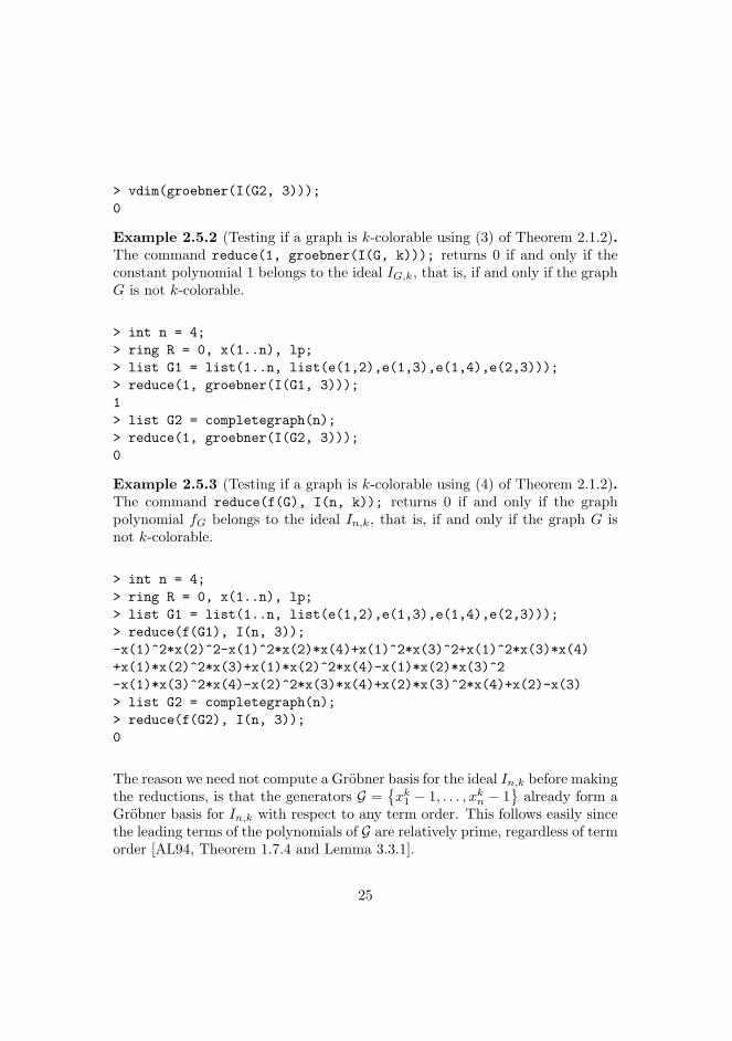
Example 2.5.2 (Testing if a graph is k-colorable using (3) of Theorem 2.1.2).The command reduce(1, groebner(I(G, k))); returns 0 if and only if theconstant polynomial 1 belongs to the ideal IG,k, that is, if and only if the graphG is not k-colorable.

> int n = 4;> ring R = 0, x(1..n), lp;> list G1 = list(1..n, list(e(1,2),e(1,3),e(1,4),e(2,3)));> reduce(1, groebner(I(G1, 3)));1> list G2 = completegraph(n);> reduce(1, groebner(I(G2, 3)));0

Example 2.5.3 (Testing if a graph is k-colorable using (4) of Theorem 2.1.2).The command reduce(f(G), I(n, k)); returns 0 if and only if the graphpolynomial fG belongs to the ideal In,k, that is, if and only if the graph G isnot k-colorable.

> int n = 4;> ring R = 0, x(1..n), lp;> list G1 = list(1..n, list(e(1,2),e(1,3),e(1,4),e(2,3)));> reduce(f(G1), I(n, 3));-x(1)^2*x(2)^2-x(1)^2*x(2)*x(4)+x(1)^2*x(3)^2+x(1)^2*x(3)*x(4)+x(1)*x(2)^2*x(3)+x(1)*x(2)^2*x(4)-x(1)*x(2)*x(3)^2-x(1)*x(3)^2*x(4)-x(2)^2*x(3)*x(4)+x(2)*x(3)^2*x(4)+x(2)-x(3)> list G2 = completegraph(n);> reduce(f(G2), I(n, 3));0

The reason we need not compute a Grobner basis for the ideal In,k before makingthe reductions, is that the generators G =

{xk1 − 1, . . . , xkn − 1

}already form a

Grobner basis for In,k with respect to any term order. This follows easily sincethe leading terms of the polynomials of G are relatively prime, regardless of termorder [AL94, Theorem 1.7.4 and Lemma 3.3.1].

25

In the last three examples – the ones regarding unique vertex colorability –we do not use the graph G2 = K4. Instead we replace it with the uniquely3-colorable graph G2 = ({1, 2, 3, 4} , {{1, 2} , {1, 3} , {1, 4} , {2, 3} , {2, 4}}).

Example 2.5.4 (Testing if a graph is uniquely k-colorable using (2) of Theo-rem 2.1.3). The command vdim(groebner(I(G, k))); returns the vector spacedimension of k[x1, . . . , xn]/IG,k over k, which is k! if and only if the graph G isuniquely k-colorable.

> int n = 4;> ring R = 0, x(1..n), lp;> list G1 = list(1..n, list(e(1,2),e(1,3),e(1,4),e(2,3)));> vdim(groebner(I(G1, 3)));12> list G2 = list(1..n, list(e(1,2),e(1,3),e(1,4),e(2,3),e(2,4)));> vdim(groebner(I(G2, 3)));6

Example 2.5.5 (Testing if a graph is uniquely k-colorable using (3) of The-orem 2.1.3). In this example we choose work with the proper 3-coloring γ ofboth G1 and G2 given by the partition {{1} , {2} , {3, 4}} of the set of vertices.Furthermore, the set {1, 2, 3} is chosen as the complete set of representatives ofthe color classes when constructing the polynomials g1, . . . , gn given by (2.4.3)in Lemma 2.4.4.

The command quotient(I(G, k), I(G, gamma)); returns a set of genera-tors of the colon ideal IG,k : IG,γ . The colon ideal equals the polynomial ringk[x1, . . . , xn] if and only if IG,γ ⊆ IG,k. Hence, the constant polynomial 1 be-longs to the colon ideal IG,k : IG,γ if and only if the polynomials g1, . . . , gnbelong to the graph ideal IG,k, that is, if and only if the graph G is uniquelyk-colorable.

> int n = 4;> ring R = 0, x(1..n), lp;> list gamma = 3, list(1, 2, intvec(3, 4));> list G1 = list(1..n, list(e(1,2),e(1,3),e(1,4),e(2,3)));> quotient(I(G1, 3), I(G1, gamma));_[1]=x(4)^3-1_[2]=x(3)^2+x(3)*x(4)+x(4)^2

26

_[3]=x(2)-x(4)_[4]=x(1)+x(3)+x(4)> list G2 = list(1..n, list(e(1,2),e(1,3),e(1,4),e(2,3),e(2,4)));> quotient(I(G2, 3), I(G2, gamma));_[1]=1

Example 2.5.6 (Testing if a graph is uniquely k-colorable using (4) of The-orem 2.1.3). In this example we choose work with the proper 3-coloring γ ofboth G1 and G2 given by the partition {{1} , {2} , {3, 4}} of the set of vertices.Furthermore, the set {1, 2, 3} is chosen as the complete set of representatives ofthe color classes when constructing the polynomials g1, . . . , gn given by (2.4.3)in Lemma 2.4.4.

The command reduce(f(G), groebner(quotient(I(n,k), I(G,gamma))));returns 0 if and only if the graph polynomial fG belongs to the ideal In,k : IG,γ ,that is, if and only if the graph G is uniquely k-colorable.

> int n = 4;> ring R = 0, x(1..n), lp;> list gamma = 3, list(1, 2, intvec(3, 4));> list G1 = list(1..n, list(e(1,2),e(1,3),e(1,4),e(2,3)));> reduce(f(G1), groebner(quotient(I(n, 3), I(G1, gamma))));-x(1)^2*x(2)^2-x(1)^2*x(2)*x(4)+x(1)^2*x(3)^2+x(1)^2*x(3)*x(4)+x(1)*x(2)^2*x(3)+x(1)*x(2)^2*x(4)-x(1)*x(2)*x(3)^2-x(1)*x(3)^2*x(4)-x(2)^2*x(3)*x(4)+x(2)*x(3)^2*x(4)+x(2)-x(3)> list G2 = list(1..n, list(e(1,2),e(1,3),e(1,4),e(2,3),e(2,4)));> reduce(f(G2), groebner(quotient(I(n, 3), I(G2, gamma))));0

2.6 Verification of a Counterexample to Xu’sConjecture

In [Xu90], Xu showed that if G is a uniquely k-colorable graph with |V | = nand |E| = m, then m ≥ (k − 1)n− k(k − 1)/2, and this bound is best possible.He went on to conjecture that if G is uniquely k-colorable with |V | = n andm = (k − 1)n − k(k − 1)/2, then G contains a k-clique. In [AMS01], thisconjecture was shown to be false for k = 3 and |V | = 24 using the graph

27

in Figure 2.2; however, the proof is somewhat complicated. We verified thatthis graph is indeed a counterexample to Xu’s conjecture using several of themethods described in Section 2.5. The fastest verification requires less thana second of processor time on a laptop PC with a 1.5 GHz Intel Pentium Mprocessor and 1.5 GB of memory running Windows Vista.

Figure 2.2: A counterexample to Xu’s conjecture [AMS01].

Below are the runtimes for the graphs in Figures 1 and 2. The term orders used isgiven using the usual Singular syntax: lp is the lexicographical ordering, Dp isthe degree lexicographical ordering, and dp is the degree reverse lexicographicalordering. All term orders ≺ used had x1 ≺ · · · ≺ xn. The symbol � indicatesthat the computation did not finish within 10 minutes.

In order to speed up the computations, basically two types of optimizationswere made to the algorithms described in Section 2.5:

(1) When computing a Grobner basis for the graph ideal IG,k in Example2.5.1, it helps to add the edges one at a time. This means that the com-mand vdim(groebner(I(G, k))); was replaced with the following pieceof code:

28

int i, j;ideal A = I(n, k);for (int l = 1; l <= size(E(G)); l++){i, j = E(G)[l];A = groebner(A + ideal(h(intvec(i,j), k - 1)));

}vdim(A);

Similar optimizations were made to the algorithms described in Examples2.5.2, 2.5.4, and 2.5.5.

(2) The number of terms in the graph polynomial fG when fully expandedmay be very large. In the algorithm described in Example 2.5.3, thereduction of the graph polynomial was therefore done iteratively. Thismeans that command reduce(f(G), I(n, k)); was replaced with thefollowing piece of code:

int i, j;poly p = 1;for (int l = 1; l <= size(E(G)); l++){i, j = E(G)[l];p = reduce((x(i) - x(j)) * p, I(n, k));

}p;

A similar optimization was made to the algorithm described in Example2.5.6.

29

Characteristic of k 0 2

Term order lp Dp dp lp Dp dp

Theorem 2.1.2 (2) 0.406 0.187 0.156 0.282 0.109 0.109Theorem 2.1.2 (3) 0.437 0.188 0.140 0.297 0.094 0.094Theorem 2.1.2 (4) 148.750 � � 43.797 558.844 �Theorem 2.1.3 (2) 0.437 0.187 0.156 0.298 0.125 0.109Theorem 2.1.3 (3) 0.453 0.204 0.171 0.297 0.157 0.108Theorem 2.1.3 (4) 161.813 � � 38.735 397.780 368.313

Runtimes in seconds for the graph in Figure 1.

Characteristic of k 0 2


Theorem 2.1.2 (2) 4.421 1.313 0.828 2.016 0.781 0.578Theorem 2.1.2 (3) 4.312 1.266 0.828 2.016 0.781 0.562Theorem 2.1.2 (4) � � � � � �Theorem 2.1.3 (2) 4.375 1.265 0.844 2.032 0.781 0.593Theorem 2.1.3 (3) 4.485 1.313 0.875 2.077 0.797 0.625Theorem 2.1.3 (4) � � � � � �

Runtimes in seconds for the graph in Figure 2.

Another way one might prove that a graph G is uniquely k-colorable is bycomputing the chromatic polynomial χG(x) and testing if it equals k! whenevaluated at x = k. This is actually possible for the graph in Figure 1. Maplereports that it has chromatic polynomial

x(x− 2)(x− 1)(x9 − 20x8 + 191x7 − 1145x6 + 4742x5

− 14028x4 + 29523x3 − 42427x2 + 37591x− 15563).

When evaluated at x = 3 we get the expected result 6 = 3!. Computing theabove chromatic polynomial took 94.83 seconds. Maple, on the other hand,was not able to compute the chromatic polynomial of the graph in Figure 2within 10 hours.

30

2.7 SINGULAR Libraries

The computer algebra system Singular1 is used extensively in this paper.Singular is especially designed for doing symbolic computations in algebra. Inparticular, it has some of the fastest routines for doing Grobner basis computa-tions which are central to the algorithms presented in this paper (see Sections2.5 and 2.6).

All the Singular examples presented in this paper use the libraries graph.liband ideals.lib described below. They are loaded with the commands:

LIB "graph.lib";LIB "ideals.lib";

Furthermore, we used the options:

option(redSB);option(noredefine);

The option redSB tells Singular to compute so-called reduced Grobner basesby default, while the option noredefine simply tells Singular not to give anywarning when variables are being redefined.

2.7.1 graph.lib

Singular does not have any built-in structures or routines for doing computa-tions with graphs. Hence, we have made our own structures.

A graph G = (V,E) is being represented by a list with two entries: V and E.The first entry V is of type intvec, which is an integer vector, while the latterentry E is of type list, which is a list of integer vectors each containing exactlytwo elements. For example, the complete graph K3 on three vertices is definedby:

1We used version 3–0–3 which is available free of charge at Singular’s homepagehttp://www.singular.uni-kl.de/.

31

intvec V = 1,2,3;list E = intvec(1,2), intvec(1,3), intvec(2,3);list K_3 = V, E;

A k-coloring of G is represented by a list with two entries: k, and a partitionP = {U1, . . . , U`} of the set V of vertices, where ` ≤ k. The first entry kis simply an integer, while the latter entry P is a list of integer vectors. Forexample, the unique proper 2-coloring γ of the path graph on four vertices isdefined by:

int k = 2;list P = intvec(1,3), intvec(2,4);list gamma = k, P;

The following code is the library graph.lib.

proc e(int i, int j){return(intvec(i, j));

}

proc graph(string G){if (G == "CC93"){intvec V = 1..12;list E = e(1,2), e(1,4), e(1,6), e(1,12), e(2,3), e(2,5),

e(2,7), e(3,8), e(3,10), e(4,9), e(4,11), e(5,6),e(5,9), e(5,12), e(6,7), e(6,10), e(7,8), e(7,11),e(8,9), e(8,12), e(9,10), e(10,11), e(11,12);

return(list(V, E));}if (G == "AMS01"){intvec V = 1..24;list E = e(1,2), e(1,4), e(1,6), e(1,12), e(2,3), e(2,7),

e(2,14), e(3,10), e(3,18), e(4,9), e(4,11), e(5,6),

32

e(5,9), e(5,12), e(6,7), e(6,10), e(7,8), e(7,11),e(7,15), e(8,9), e(8,12), e(10,11), e(10,14),e(10,22), e(11,12), e(13,14), e(13,16), e(13,18),e(13,24), e(14,15), e(14,19), e(15,22), e(16,21),e(16,23), e(17,18), e(17,21), e(17,24), e(18,19),e(18,22), e(19,20), e(19,23), e(20,21), e(20,24),e(22,23), e(23,24);

return(list(V, E));}

}

proc f(list G){int i, j;poly p = 1;for (int l = 1; l <= size(E(G)); l++){i, j = E(G)[l];p = p * (x(i) - x(j));

}return(p);

}

proc V(list G){return(G[1]);

}

proc E(list G){return(G[2]);

}

proc pathgraph(int n){list E;for (int i = 1; i < n; i++) { E = E + list(e(i, i + 1)); }return(list(1..n, E));

}

33

proc completegraph(int n){list E;for (int i = 1; i < n; i++){for (int j = i + 1; j <= n; j++) { E = E + list(e(i, j)); }

}return(list(1..n, E));

}

2.7.2 ideals.lib

Recall that for a subset U ⊆ V of vertices and a positive integer d, hdU is thesum of all monomials of degree d in the indeterminates {x` : ` ∈ U}. We mayalso express hdU as

hdU =d∑

l=0

xlihd−lU\{i}

for any i ∈ U . This is the expression used to construct hdU recursively in theprocedure h below. The following code is the library ideals.lib.

proc h(intvec U, int d){if (size(U) == 1) { return(x(U[1])^d); }poly p;for (int l = 0; l <= d; l++){p = p + x(U[1])^l * h(intvec(U[2..size(U)]), d - l);

}return(p);

}

proc v(list gamma, intvec U, int i){int j1, j2, j3, j4;for (j1 = 1; j1 <= size(gamma[2]); j1++)

34

{for (j2 = 1; j2 <= size(gamma[2][j1]); j2++){if (i == gamma[2][j1][j2]){for (j3 = 1; j3 <= size(gamma[2][j1]); j3++){

for (j4 = 1; j4 <= size(U); j4++){if (U[j4] == gamma[2][j1][j3]) { return(U[j4]); }

}}

}}

}}

proc g(list gamma, int i){int j;int k = gamma[1];int l = size(gamma[2]);intvec U;U[1] = gamma[2][1][1];for (j = 2; j <= l; j++) { U = U, gamma[2][j][1]; }if (i == U[1]) { return(x(U[1])^k - 1); }for (j = 2; j <= l; j++){if (i == U[j]) { return(h(intvec(U[1..j]), k + 1 - j)); }

}return(x(i) - x(v(gamma, U, i)));

}

proc I(expr1, expr2){int i, j;ideal A;if (typeof(expr1) == "int"){

35

int n = expr1;int k = expr2;for (i = 1; i <= n; i++) { A[i] = x(i)^k - 1; }return(A);

}list G = expr1;int n = size(V(G));if (typeof(expr2) == "int"){int k = expr2;for (int l = 1; l <= size(E(G)); l++){i, j = E(G)[l];A[l] = (x(i)^k - x(j)^k) / (x(i) - x(j));

}return(I(n, k) + A);

}list gamma = expr2;for (i = 1; i <= n; i++) { A[i] = g(gamma, i); }return(A);

}

36

II

The Quillen–SuslinTheorem

37

Part 3

Revisiting anAlgorithm for theQuillen–Suslin Theorem

We give a new constructive algorithm for the Quillen–Suslin Theorem in the im-portant case of an infinite ground field. The new algorithm follows the lines of analgorithm by Logar and Sturmfels, but differs in the way it constructs sequencesof polynomials and matrices that are central to the algorithm. The output ofthe two algorithms are not easily comparable, however, both theoretical and ex-perimental evidence that the new algorithm produces a much simpler output, ispresented. Some tricks that may potentially simplify the computations furtheras well as some drawbacks of the algorithms are also discussed.

38

3.1 Introduction

Let k be a field, and let k[x1, . . . , xn] be the polynomial ring over k in inde-terminates x1, . . . , xn. The following theorem, known as Serre’s Conjecture, iscentral in commutative algebra.

Theorem 3.1.1 (Serre’s Conjecture). Every finitely generated projective moduleover k[x1, . . . , xn] is free.

It was proved independently by Quillen and Suslin in 1976. We refer to the book[Lam06] by Lam for more information on Serre’s Conjecture and its history.

A matrix over a commutative ring is said to be unimodular if its maximalminors generate the unit ideal. Serre’s Conjecture is equivalent to the followingtheorem.

Theorem 3.1.2 (Quillen–Suslin). For every unimodular `×m matrix F (with` ≤ m) over k[x1, . . . , xn], there exists a unimodular m × m matrix U overk[x1, . . . , xn] such that

FU =

1 0 0 · · · 0. . .

.... . .

...0 1 0 · · · 0

.

For a commutative ring A, and a multiplicative closed subset S ⊆ A, let S−1Adenote the ring S−1A = {a/s : a ∈ A and s ∈ S}. In case S =

{s, s2, . . .

}for

some s ∈ A\ {0}, we simply write s−1A instead of S−1A.

In 1992, Logar and Sturmfels [LS92] gave a constructive algorithm for theQuillen–Suslin Theorem in case k = C. An analysis of the algorithm showsthat what is central for the construction of such a unimodular m×m matrix U ,is the ability to construct polynomials r1, . . . , rk ∈ k[x1, . . . , xn−1], and matricesUi over r−1

i k[x1, . . . , xn] for each i = 1, . . . , k such that

1. the polynomials r1, . . . , rk generate k[x1, . . . , xn−1],

2. the row fUi is over r−1i k[x1, . . . , xn−1], and

3. the matrix Ui is unimodular,

39

for any positive integer n, and any unimodular row f =(f1 · · · fm

)over

k[x1, . . . , xn].

The organization of this paper is as follows. In Section 3.2, we give a newconstructive algorithm for the Quillen–Suslin Theorem in the important case ofan infinite ground field k. We do so by constructing sequences of polynomialsr1, . . . , rk and matrices U1, . . . , Uk with the above three properties. The outputof the two algorithms are not easily comparable. The new algorithm, however,almost certainly produces a much simpler output. Theoretical and experimentalevidence to support this claim, is presented in Section 3.3. Finally, in Section 3.4,we discuss some tricks that may potentially simplify the computations furtheras well as some drawbacks of the algorithms.

3.2 Algorithm for theUnimodular Row Problem

The problem of constructing a unimodular m×m matrix U as in Theorem 3.1.2may be reduced to the following using induction (see [LS92] for details).

Problem 3.2.1 (Unimodular Row Problem). Given a unimodular row f =(f1 · · · fm

)over k[x1, . . . , xn], find a unimodular m × m matrix U over

k[x1, . . . , xn] such that fU =(

1 0 · · · 0).

Let A be a commutative ring, and suppose f =(f1 · · · fm

)is a uni-

modular row overA[x] in which f1 is monic. We begin by computing polynomialsg1, . . . , gm ∈ A[x] such that

f1g1 + · · ·+ fmgm = 1.

In case m = 2, the matrix U over A[x] defined by

U =(g1 −f2

g2 f1

)

satisfies fU =(

1 0). Hence, from now on, we may assume that m ≥ 3. We

will need the following result by Lombardi and Yengui.

40

Theorem 3.2.2 ([LY05, Corollary 3]). Let k = deg(f1) + 1 and suppose Acontains a set {a1, . . . , ak} such that the difference between any two elements isinvertible. Then 〈r1, . . . , rk〉 = A, where

ri = Res

f1, f2 + ai

m∑

j=3

fjgj

∈ A.

For our application, A will be a polynomial ring over an infinite field. Hence, wemay choose such a set {a1, . . . , ak}, and compute the resultants r1, . . . , rk ∈ Adefined in the theorem. If the resultant ri is zero for some i, it may simply bediscarded. Thus, we may assume, without loss of generality, that ri is nonzerofor i = 1, . . . , k. Furthermore, find s1, . . . , sk ∈ A such that

r1s1 + · · ·+ rksk = 1.

For each i = 1, . . . , k we now compute polynomials pi, qi ∈ A[x] such that

pif1 + qi

f2 + ai

m∑

j=3

fjgj

= ri,

and construct the following matrix Mi over A[x]:

Mi =

f1 f2 f3 · · · fm−qi pi 0 · · · 00 −aig3 1 · · · 0...

......

. . ....

0 −aigm 0 · · · 1

.

An obvious property of Mi which will be important later on, is that(

1 0 · · · 0)Mi = f. (3.2.1)

We claim that Mi has determinant ri. To see this, simply expand the determi-nant along the first row:

det(Mi) = pif1 − (−qi)f2 +m∑

j=3

(−1)1+j(−qi)fj((−1)j−1aigj) = ri.

Since ri is nonzero, Mi is invertible when considered as a matrix over r−1i A[x].

Hence, we let Ui = M−1i over r−1

i A[x].

41

Remark 3.2.3. Notice that in case ri is invertible, the matrix Ui is in fact overA[x], and satisfies fUi =

(1 0 · · · 0

).

It is straight forward to verify that Ui = Im − r−1i Ni , where Im is the m ×m

identity matrix, and Ni is the following matrix over A[x]:

Ni =

ri − pi f2 + ai∑mj=3 fjgj pif3 · · · pifm

− qi ri − f1 qif3 · · · qifm−aiqig3 −aif1g3 aiqif3g3 · · · aiqifmg3

......

.... . .

...−aiqigm −aif1gm aiqif3gm · · · aiqifmgm

.

This explicit expression of Ui may be useful when implementing the algorithmfor the Unimodular Row Problem described below, but we shall not need it. Wemay now construct the matrix ∆i over r−1

i A[y, z]:

∆i = Ui (y) · U−1i (y + z).

It is clear that ∆i has determinant 1, and that ∆i(y, 0) = Im. It follows from(3.2.1) that ∆i has the property

f(y)∆i = f(y + z). (3.2.2)

Recall that the matrix Mi is defined over A[x] and has determinant ri. SinceUi equals the adjoint of Mi divided by the determinant of Mi, we see that ri isa common denominator for all the entries of Ui. This means that ri is also acommon denominator for all the entries of ∆i. Expanding the matrix

∆i = Im + ∆i1z + ∆i2z2 + · · ·+ ∆idiz

di

as a polynomial in z with matrix coefficients over r−1i A[y] shows that replacing

z by riz yields a matrix ∆i(y, riz) over A[y, z]. We may now finally constructthe matrix V over A[x] as follows:

V = ∆1(x,−r1s1x)k∏

i=2

∆i

((1−

i−1∑

t=1

rtst

)x,−risix

).

It is clear that V has determinant 1. Furthermore, it follows from (3.2.2) that Vhas the property that, when multiplied by the unimodular row f , it will evaluate

42

f at x = 0:

fV = f(x− r1s1x)k∏

i=2

∆i

((1−

i−1∑

t=1

rtst

)x,−risix

)

= f

((1−

k∑

t=1

rtst

)x

)

= f(0).

The construction of V form the basis of the following algorithm for the Uni-modular Row Problem. In what follows, k is an infinite field.

Algorithm 3.2.4. With the above notation, we have the following algorithmfor the Unimodular Row Problem:

Input: A unimodular row f =(f1 · · · fm

)over k[x1, . . . , xn] with m ≥ 3.

Output: A unimodular m×m matrix U over k[x1, . . . , xn] such that

fU =(

1 0 · · · 0).

1. Let U := Im be the m×m identity matrix.

2. Let A := k[x1, . . . , xn−1] and x := xn, and consider f as a row over A[x].

3. Using Noether normalization, make a linear change of variables such thatf1 becomes monic, and update U accordingly.

4. Let k := deg(f1) + 1, and choose a set {a1, . . . , ak} ⊆ A such that thedifference between any two elements is invertible.

5. Compute polynomials g1, . . . , gm ∈ A[x] such that f1g1 + · · ·+ fmgm = 1.

6. For each i = 1, . . . , k do:

(a) Compute the resultant ri = Res(f1, f2 + ai

∑mj=3 fjgj

)∈ A.

(b) Compute pi, qi ∈ A[x] such that pif1 + qi

(f2 + ai

∑mj=3 fjgj

)= ri.

(c) If ri is invertible, let U := UUi and exit the algorithm.

7. Compute polynomials s1, . . . , sk ∈ A such that r1s1 + · · ·+ rksk = 1.

43

8. Let U := UV , and let f := fV .

9. Let n := n− 1, and go to step 2.

Proof. The algorithm will terminate once an invertible ri has been found. Thiswill happen sooner or later, since if n = 1 is reached, then r1, . . . , rk ∈ k willgenerate k by Theorem 3.2.2. Hence, there is some nonzero ri. It follows fromthe above construction of V and Remark 3.2.3 that the algorithm produces aunimodular m×m matrix such that fU =

(1 0 · · · 0

). We note that the

new row f in step 8 is again unimodular since fV = f(0), and

f1(0)g1(0) + · · ·+ fm(0)gm(0) = 1(0) = 1.

This completes the proof.

3.3 Complexity

We have seen that ri is a common denominator for all the entries of ∆i, whichimplies that by replacing z by riz, we get a matrix ∆i(y, riz) over A[y, z]. Inthe algorithm by Logar and Sturmfels we, however, need to replace z by rmi z inorder to get rid of the denominators. This has a huge impact on the resultingunimodular m × m matrix U . Not only because z in ∆i, when constructingV , gets replaced by rmi s

′ix instead of risix, but also because the polynomials

s′1, . . . , s′k needed in order for

rm1 s′1 + · · ·+ rmk s

′k = 1

also get much more complicated with bigger coefficients and higher degrees asa result. We shall now see an example of this.

Example 3.3.1. Let f =(x2

2 x21 + x2 x1x2 + x1 + x2 + 1

)be a row over

k[x1, x2]. We verify that f is indeed unimodular and compute the polynomialsg1, g2, g3 ∈ k[x1, x2] using a Grobner basis computation in Maple:

[> with(LinearAlgebra):[> with(Groebner):[> f := [x[2]^2, x[1]^2+x[2], x[1]*x[2]+x[1]+x[2]+1];[> g := Basis(f, plex(x[1],x[2]), output=extended)[2][];

44

We get the row g =(

2 + x2x21 − x2 − x2

1 −x2 + 1 −(x2 − 1)2(−1 + x1)),

and may verify that f (and g) is unimodular since f1g1 + f2g2 + f3g3 = 1. Welet k = 3, and choose a1 = 0, a2 = 1, and a3 = 2. Next we compute theresultant r1, and the polynomials p1, and q1:

[> a := [0, 1, 2];[> r[1] := resultant(f[1], f[2]+a[1]*f[3]*g[3], x[2]);[> pq := Basis([f[1], f[2]+a[1]*f[3]*g[3]],

plex(x[2]), output=extended)[2][];[> p[1] := pq[1]*r[1];[> q[1] := pq[2]*r[1];

This yields r1 = x41, p1 = 1, and q1 = −x2 + x2

1. Since r1 is not invertible, wecompute the resultant r2, and the polynomials p2, and q2:

[> r[2] := resultant(f[1], f[2]+a[2]*f[3]*g[3], x[2]);[> pq := Basis([f[1], f[2]+a[2]*f[3]*g[3]],

plex(x[2]), output=extended)[2][];[> p[2] := pq[1]*r[2];[> q[2] := pq[2]*r[2];

This then yields r2 = 1, p2 = x41 − x4

1x22 + x2

2x21 + x4

1x2 − x2 − x21 + 1, and

q2 = −x2x21 + 1. Since r2 is invertible, it follows from Remark 3.2.3 that U2

satisfies fU2 =(

1 0 0). We therefore compute U2:

[> M[2] := Matrix(3, 3, [[f[1], f[2], f[3]],[-q[2], p[2], 0], [0, -a[2]*g[3], 1]]);

[> U[2] := M[2]^(-1);

45

The result is the 3× 3 matrix U2 = (uij) in which

u11 = x41 − x4

1x22 + x2

2x21 + x4

1x2 − x2 − x21 + 1,

u21 = −x2x21 + 1,

u31 = (−1 + x2x21)(x2

2x1 − 2x1x2 + 2x2 − x22 − 1 + x1),

u12 = x21x

32 − x2

2x21 − x2x

21 + x2

2 − x32 − 1,

u22 = x22,

u32 = −x22(x2

2x1 − 2x1x2 + 2x2 − x22 − 1 + x1),

u13 = (x1x2 + x1 + x2 + 1)(−x41 + x4

1x22 − x2

2x21 − x4

1x2 + x2 + x21 − 1),

u23 = (x1x2 + x1 + x2 + 1)(−1 + x2x21),

u33 = x41x

22 − x4

2x41 + x4

2x21 + x3

2x41 − x3

2 − 2x22x

21 + x2

2 + x21 + x2 − x4

1x2.

One may also verify that this matrix has determinant 1, and so is indeed uni-modular. Notice that the entries of U2 have degree ranging from 2 to 8.

If we assume that k has characteristic zero, the algorithm by Logar and Sturm-fels, given the same input as before, produces another unimodular 3× 3 matrixwith entries

u11 = c1x911 x

42 + (635 terms),

u21 = −c1x891 x

62 + (714 terms),

u31 = c1x891 x

62 + (719 terms),

u12 = c1x921 x

42 + (645 terms),

u22 = −c1x901 x

62 + (727 terms),

u32 = c1x901 x

62 + (729 terms),

u13 = −c2x671 x

32 + (394 terms),

u23 = c2x651 x

52 + (303 terms),

u33 = −c2x651 x

52 + (303 terms),

in which

c1 = 75346795455490677117212220114576

+ 33696111280109816482971698230272√

5,c2 = 1780395043182825433742028

+ 796216849068911274481428√

5.

46

The degree of the entries of the above matrix range from 70 to 96. Thus, thealgorithm by Logar and Sturmfels leads to a tremendous growth in both thecoefficients as well as the degrees. Another unfortunate aspect is the introduc-tion of

√5 in the solution keeping in mind that we may view f as a row over

Q[x1, x2]. This is due to the fact the algorithm by Logar and Sturmfels onlyworks for an algebraically closed field k.

3.4 Tricks and Drawbacks

We conclude with some tricks that may potentially simplify the computationsneeded to find a unimodular m×m matrix U as in Theorem 3.1.2, when given aconcrete unimodular row f =

(f1 · · · fm

)over k[x1, . . . , xn]. Some draw-

backs of the algorithms are also discussed.

(1) If we compute polynomials g1, . . . , gm such that f1g1+· · ·+fmgm = 1, andone of the gj is a nonzero element of k, then U may easily be constructedas a product of elementary column operations matrices.

(2) Given f , we may try to divide each fj by {f1, . . . , fj−1, fj+1, . . . , fm} usingthe division algorithm. Suppose, for instance,

f1 = h2f2 + · · ·+ hmfm + r

for polynomials h2, . . . , hm not all zero, and a remainder r. The row f maythen easily be replaced by

(r f2 · · · fm

)using elementary column

operations. We may then try to divide f2, and so on. In the end we areleft with a unimodular row f ′ =

(f ′1 · · · f ′m

)which may hopefully

lead to a simpler output of Algorithm 3.2.4.

(3) For an elementary column operation matrix E, let Uf and UfE be theoutput produced by Algorithm 3.2.4 for the unimodular rows f and fE,respectively. It would be desirable to have UfE = UfE, however, this isnot the case. As an example we may interchange the first two columnsof f in Example 3.3.1. Algorithm 3.2.4 now produces a unimodular 3× 3matrix the entries of which have degree ranging from 25 to 28. This isalso a drawback of the algorithm by Logar and Sturmfels.

47

(4) The output of Algorithm 3.2.4 strongly depends on the choice of subset{a1, . . . , ak} made in each iteration. It is natural to prefer small valuesfor the ai in order to prevent coefficient growth. However, for a given uni-modular row, there might be some other choice for the ai that yields par-ticularly simple resultants. If so, Algorithm 3.2.4 may terminate sooner,hopefully producing a simpler output.

48

III

Symmetric Ideals

49

Part 4

Minimal Generators forSymmetric Ideals

Let R = k[X] be the polynomial ring in infinitely many indeterminates X over afield k, and let SX be the symmetric group of X. The group SX acts naturallyon R, and this in turn gives R the structure of a module over the group ringR[SX ]. A recent theorem of Aschenbrenner and Hillar states that the moduleR is Noetherian. We address whether submodules of R can have any number ofminimal generators, answering this question positively.

50

4.1 Introduction

Let R = k[X] be the polynomial ring in infinitely many indeterminates X over afield k, and let SX be the symmetric group of X. The group SX acts naturallyon R: if σ ∈ SX and f ∈ k[x1, . . . , x`] where xi ∈ X, then

σf(x1, x2, . . . , x`) = f(σx1, σx2, . . . , σx`) ∈ R. (4.1.1)

We say that an ideal I ⊆ R is symmetric if I is invariant under SX , that is, if

SXI = {σf : σ ∈ SX , f ∈ I} ⊆ I.

The action (4.1.1) naturally gives R the structure of a (left) module over the(left) group ring R[SX ] defined by

R[SX ] =

{finite∑

σ∈SX

rσσ : rσ ∈ R}.

Symmetric ideals are then simply the submodules of R. Aschenbrenner andHillar recently proved the following.

Theorem 4.1.1. Every symmetric ideal of R is finitely generated as an R[SX ]-module. In other words, R is a Noetherian R[SX ]-module.

Theorem 4.1.1 was motivated by finiteness questions in chemistry and algebraicstatistics (see the references in [AH07]).

The basic question whether a symmetric ideal is always cyclic (already askedby J. Schicho1) was left unanswered in [AH07]. Our result addresses a general-ization of this important issue.

Theorem 4.1.2. For every positive integer n, there are symmetric ideals of Rgenerated by n polynomials which cannot have fewer than n R[SX ]-generators.

At first glance, Theorem 4.1.2 is a bit surprising. If one picks even a singlepolynomial g ∈ R, the cyclic submodule 〈g〉 is very large, and it is not clearthat every submodule of R doesn’t arise in this way. Given a finite list of

1Private communication, 2006.

51

polynomials f1, . . . , fn, one could conceivably choose a sufficiently large enoughpositive integer N so that the number of unknowns in a system

f1 =∑

σ∈SN

r1σσg, r1σ ∈ R

...

fn =∑

σ∈SN

rnσσg, rnσ ∈ R

greatly outnumbers the number of equations, thereby (presumably) ensuring asolution for the riσ. Here SN denotes the set of permutations of {1, . . . , N}.

In what follows, we work with the setX = {x1, x2, x3, . . .}, although as remarkedin [AH07], this is not really a restriction. In this case, SX is naturally identifiedwith S∞, the permutations of the set of positive integers, and σxi = xσi forσ ∈ S∞.

4.2 Multisets and monomials

In this section, we provide the basic notation used in the proof of Theorem 4.1.2as well as the proof itself.

Formally, a multiset M = (A,m) is a set A along with a multiplicity functionm : A → Z which assigns to each element a ∈ A a nonnegative multiplicitym(a).

In what follows, the set A will always be the set of positive integers and m willbe a function with finite support; that is, m will be nonzero for only finitelymany elements of A. For notational simplicity, we will frequently view M as afinite set of positive integers with repetitions allowed as in M = {1, 1, 1, 2, 3, 3}.

Multisets are in natural bijection with monomials of R. Given a multiset M =(A,m), we can construct the monomial:

xM =∏

a∈Axm(a)a .

Conversely, given a monomial, the associated multiset is the set of indices ap-pearing in it, along with multiplicities.

52

Let M = (A,m) be a multiset and let a1, . . . , ak be the list elements of A withpositive multiplicity, arranged so that m(a1) ≥ · · · ≥ m(ak). The type of amultiset M (or the corresponding monomial) is the vector

λ(M) = (m(a1), . . . ,m(ak)).

For instance, the multiset M = {1, 1, 1, 2, 3, 3} has type λ(M) = (3, 2, 1). Theaction of S∞ on monomials coincides with the natural action of S∞ on multisetsM = (A,m): σM = (A, σm), in which σm : A→ Z is the function i 7→ m(σ−1i).It easy to see that the action of S∞ preserves the type of a monomial.

We also note that an infinite permutation acting on a polynomial may be re-placed with a finite one.

Lemma 4.2.1. Let σ ∈ S∞ and f ∈ R. Then there exists a positive integer Nand τ ∈ SN such that τf = σf .

Proof. Let S be the set of indices appearing in the monomials of f and let Nbe the largest integer in σS ∪ S. The injective function σ|S : S → {1, . . . , N}extends (nonuniquely) to a permutation τ ∈ SN such that τf = σf .

We will derive Theorem 4.1.2 is a direct corollary of the following result.

Theorem 4.2.2. Let G = {g1, . . . , gn} be a set of monomials of degree d withdistinct types and fix an n × n matrix C = (cij) over k of rank r. Then thesubmodule I = 〈f1, . . . , fn〉 of R generated by the n polynomials

fj =n∑

i=1

cijgi, j = 1, . . . , n

cannot have fewer than r R[S∞]-generators.

Proof. Suppose that p1, . . . , pk are generators for I = 〈f1, . . . , fn〉 with the fj asin the statement of the theorem; we prove that k ≥ r. Note that each nonzerofj is homogeneous of degree d. Since each pl ∈ I, it follows that each is alinear combination, over R[S∞], of monomials in G. Therefore, each monomialoccurring in pl has degree at least d, and, moreover, any degree d monomial inpl has the same type as one of the monomials in G.

53

Write each of the monomials in G in the form gi = xMifor multisets M1, . . . ,Mn

with corresponding distinct types λ1, . . . , λn. Then we can express each gene-rator pl in the following form:

pl =n∑

i=1

∑

λ(M)=λi

uilMxM + ql, (4.2.1)

in which uilM ∈ k with only finitely many of them nonzero, each monomialappearing in ql has degree greater than d, and the inner sum is over all multisetsM with type λi.

Since each polynomial in {f1, . . . , fn} is a finite linear combination of the pl, andsince only finitely many positive integers are indices of monomials appearing inp1, . . . , pk, it follows that we may pick a positive integer N large enough so thatall of these linear combinations can be expressed with coefficients in the subringR[SN ] (c.f. Lemma 4.2.1). Therefore, we have

fj =k∑

l=1

∑

σ∈SN

sljσσpl, (4.2.2)

for some polynomials sljσ ∈ R. Substituting the expressions found in (4.2.1)into (4.2.2) produces

fj =k∑

l=1

∑

σ∈SN

sljσ

n∑

i=1

∑

λ(M)=λi

uilMxσM + σql

=k∑

l=1

∑

σ∈SN

n∑

i=1

∑

λ(M)=λi

vljσuilMxσM + hj ,

in which each monomial appearing in hj ∈ R has degree greater than d andvljσ is the constant term of sljσ. Since each fj has degree d, we must have thathj = 0. It follows that

n∑

i=1

cijxMi=

k∑

l=1

∑

σ∈SN

n∑

i=1

∑

λ(M)=λi

vljσuilMxσM .

Next, for a fixed i, take the sum on each side in this last equation of the coeffi-

54

cients of monomials with the type λi. This produces the n2 equations:

cij =k∑

l=1

∑

σ∈SN

∑

λ(M)=λi

vljσuilM

=k∑

l=1

∑

λ(M)=λi

uilM

( ∑

σ∈SN

vljσ

)

=k∑

l=1

UilVlj ,

(4.2.3)

in whichUil =

∑

λ(M)=λi

uilM and Vlj =∑

σ∈SN

vljσ.

Let U be the n× k matrix (Uil) and similarly let V be the k × n matrix (Vlj).The n2 equations (4.2.3) can be viewed compactly as matrix multiplication:

c11 · · · c1n...

. . ....

cn1 · · · cnn

=

U11 · · · U1k

.... . .

...Un1 · · · Unk

V11 · · · V1n

.... . .

...Vk1 · · · Vkn

.

Considering the rank of both sides of the equation C = UV leads to the followingchain of inequalities:

r = rank(C) = rank(UV ) ≤ min{rank(U), rank(V )} ≤ min{n, k} ≤ k.

Therefore, we have k ≥ r, and this completes the proof.

Example 4.2.3. According to Theorem 4.2.2, the submodule I =⟨x1x2, x

21

⟩

of R cannot have fewer than two R[S∞]-generators. Thus, I is an example of anoncyclic symmetric ideal.

Proof of Theorem 4.1.2. Let gi = xi1x2 · · ·xn+1−i and apply Theorem 4.2.2 withC being the n× n identity matrix.

55

Bibliography

[AH07] Matthias Aschenbrenner and Christopher J. Hillar. Finite generationof symmetric ideals. Trans. Amer. Math. Soc., 359(11):5171–5192,2007.

[AL94] William W. Adams and Philippe Loustaunau. An introduction toGrobner bases, volume 3 of Graduate Studies in Mathematics. Amer-ican Mathematical Society, Providence, RI, 1994.

[AMS01] S. Akbari, V. S. Mirrokni, and B. S. Sadjad. Kr-free uniquely vertexcolorable graphs with minimum possible edges. J. Combin. TheorySer. B, 82(2):316–318, 2001.

[AT92] N. Alon and M. Tarsi. Colorings and orientations of graphs. Combi-natorica, 12(2):125–134, 1992.

[Bay82] David Allen Bayer. The Division Algorithm and the Hilbert Scheme.PhD thesis, Harvard University, Department of Mathematics, June1982.

[CC93] Chong-Yun Chao and Zhibo Chen. On uniquely 3-colorable graphs.Discrete Math., 112(1-3):21–27, 1993.

[CLO05] David A. Cox, John Little, and Donal O’Shea. Using algebraic geo-metry, volume 185 of Graduate Texts in Mathematics. Springer, NewYork, second edition, 2005.

[CLO07] David Cox, John Little, and Donal O’Shea. Ideals, varieties, and al-gorithms. Undergraduate Texts in Mathematics. Springer, New York,third edition, 2007. An introduction to computational algebraic geo-metry and commutative algebra.

56

[Cox] David Cox. Private communication, 2007.

[dL95] Jesus A. de Loera. Grobner bases and graph colorings. BeitrageAlgebra Geom., 36(1):89–96, 1995.

[DPT03] Klaus Dohmen, Andre Ponitz, and Peter Tittmann. A new two-variable generalization of the chromatic polynomial. Discrete Math.Theor. Comput. Sci., 6(1):69–89 (electronic), 2003.

[Kos01] Thomas Koshy. Fibonacci and Lucas numbers with applications. Pureand Applied Mathematics (New York). Wiley-Interscience, New York,2001.

[KR00] Martin Kreuzer and Lorenzo Robbiano. Computational commutativealgebra. 1. Springer-Verlag, Berlin, 2000.

[Lam06] T. Y. Lam. Serre’s problem on projective modules. Springer Mono-graphs in Mathematics. Springer-Verlag, Berlin, 2006.

[LS92] Alessandro Logar and Bernd Sturmfels. Algorithms for the Quillen-Suslin theorem. J. Algebra, 145(1):231–239, 1992.

[LY05] Henri Lombardi and Ihsen Yengui. Suslin’s algorithms for reductionof unimodular rows. J. Symbolic Comput., 39(6):707–717, 2005.

[Xu90] Shao Ji Xu. The size of uniquely colorable graphs. J. Combin. TheorySer. B, 50(2):319–320, 1990.

57

Summary in English

Part 1 introduces a simple idea that relates graph coloring with certain integersequences including the Fibonacci and Lucas numbers. It demonstrates how onecan produce identities involving these numbers by decomposing different classesof graphs in different ways. Part 2 deals with graph coloring from a compu-tational algebraic point of view. It collects a series of results in the literatureregarding graphs that are not k-colorable, and provides a refinement to uniquelyk-colorable graphs. It also gives algorithms for testing (unique) vertex colorabil-ity. Part 3 provides a new algorithm for the Quillen–Suslin Theorem in case ofan infinite ground field. The new algorithm follows the lines of an algorithm byLogar and Sturmfels, however, both theoretical and experimental evidence thatthe new algorithm produces a much simpler output, is presented. Part 4 settlesa question regarding the minimal number of generators for symmetric ideals inpolynomial rings with infinitely many indeterminates.

58

Summary in Danish

Del 1 introducerer en simpel ide som skaber en forbindelse mellem graffarvningog udvalgte følger af heltal herunder Fibonacci og Lucas tallene. Den demon-strerer hvorledes man kan producere identiteter, som involverer disse tal, ved atdekomponere forskellige familier af grafer pa forskellige mader. Del 2 omhand-ler graffarvning fra et beregningsmæssigt algebraisk synspunkt. Den samler enrække resultater fra litteraturen vedrørende grafer der ikke er k-farvbare, oggiver en specialicering til entydigt k-farvbare grafer. Den giver ligeledes algo-ritmer til at teste om en graf er (entydig) knudefarvbar. Del 3 giver en nyalgoritme for Quillen–Suslins sætning i tilfældet af et uendeligt grundlegeme.Den nye algoritme følger konstruktionen af en algoritme af Logar og Sturm-fels, men bade teoretiske og eksperimentielle argumenter der indikerer at dennye algoritme producerer et meget simplere output, bliver præsenteret. Del 4giver svaret pa et spørgsmal vedrørende det minimale antal frembringere forsymmetriske idealer i polynomiumsringe med uendeligt mange variable.

59

Papers to appear

60

FIBONACCI IDENTITIES AND GRAPH COLORINGS

CHRISTOPHER J. HILLAR AND TROELS WINDFELDT

Abstract. We generalize both the Fibonacci and Lucas numbers to the context of graphcolorings, and prove some identities involving these numbers. As a corollary we obtain newproofs of some known identities involving Fibonacci numbers such as


1. Introduction

In graph theory, it is natural to study vertex colorings, and more specifically, those col-orings in which adjacent vertices have different colors. In this case, the number of suchcolorings of a graph G is encoded by the chromatic polynomial of G. This object can becomputed using the method of “deletion and contraction”, which involves the recursive com-bination of chromatic polynomials for smaller graphs. The purpose of this note is to showhow the Fibonacci and Lucas numbers (and other integer recurrences) arise naturally in thiscontext, and in particular, how identities among these numbers can be generated from thedifferent choices for decomposing a graph into smaller pieces.

We first introduce some notation. Let G be a undirected graph (possibly containing loopsand multiple edges) with vertices V = {1, . . . , n} and edges E. Given nonnegative integersk and �, a (k, �)-coloring of G is a map

ϕ : V → {c1, . . . , ck+�},in which {c1, . . . , ck+�} is a fixed set of k+� “colors”. The map ϕ is called proper if wheneveri is adjacent to j and ϕ(i), ϕ(j) ∈ {c1, . . . , ck}, we have ϕ(i) �= ϕ(j). Otherwise, we say thatthe map ϕ is improper. In somewhat looser terminology, one can think of {ck+1, . . . , ck+�}as coloring “wildcards”.

Let χG(x, y) be a function such that χG(k, �) is the number of proper (k, �)-colorings ofG. This object was introduced by the authors of [2] and can be given as a polynomial inx and y (see Lemma 1.1). It simultaneously generalizes the chromatic, independence, andmatching polynomials of G. For instance, χG(x, 0) is the usual chromatic polynomial whileχG(x, 1) is the independence polynomial for G (see [2] for more details).

We next state a simple rule that enables one to calculate the polynomial χG(x, y) recur-sively. In what follows, G\e denotes the graph obtained by removing the edge e from G, andfor a subgraph H of G, the graph G\H is gotten from G by removing H and all the edgesof G that are adjacent to vertices of H. Additionally, the contraction of an edge e in G isthe graph G/e obtained by removing e and identifying as equal the two vertices sharing thisedge.

The first author is supported under a National Science Foundation Postdoctoral Fellowship.

MAY 2008/2009 1

THE FIBONACCI QUARTERLY

Lemma 1.1. Let e be an edge in G, and let v be the vertex to which e contracts in G/e.Then,

χG(x, y) = χG\e(x, y)− χG/e(x, y) + y · χ(G/e)\v(x, y). (1.1)

Proof. The number of proper (k, �)-colorings of G\e which have distinct colors for the verticessharing edge e is given by χG\e(k, �)− χG/e(k, �); these colorings are also proper for G. Theremaining proper (k, �)-colorings of G are precisely those for which the vertices sharing edgee have the same color. This color must be one of the wildcards {ck+1, . . . , ck+�}, and so thenumber of remaining proper (k, �)-colorings of G is counted by � · χ(G/e)\v(k, �). �

With such a recurrence, we need to specify initial conditions. When G simply consists ofone vertex and has no edges, we have χG(x, y) = x + y, and when G is the empty graph,we set χG(x, y) = 1 (consider G with one edge joining two vertices in (1.1)). Moreover, χis multiplicative on disconnected components. This allows us to compute χG for any graphrecursively.

In the special case when k = 1, there is also a way to calculate χG(1, y) by removingvertices from G. Define the link of a vertex v to be the subgraph link(v) of G consisting ofv, the edges touching v, and the vertices sharing one of these edges with v. Also if u and vare joined by an edge e, we define link(e) to be link(u)∪ link(v) in G, and also we set deg(e)to be deg(u) + deg(v)− 2. We then have the following rules.

Lemma 1.2. Let v be any vertex of G, and let e be any edge. Then,

χG(1, y) = y · χG\v(1, y) + ydeg(v) · χG\link(v)(1, y), (1.2)

χG(1, y) = χG\e(1, y)− ydeg(e) · χG\link(e)(1, y). (1.3)

Proof. The number of proper (1, �)-colorings of G with vertex v colored with a wildcard is� ·χG\v(1, �). Moreover, in any proper coloring of G with v colored c1, each vertex among thedeg(v) ones adjacent to v can only be one of the � wildcards. This explains the first equalityin the lemma.

Let v be the vertex to which e contracts in G/e. From equation (1.2), we have

χG/e(1, y) = y · χ(G/e)\v(1, y) + ydeg(v) · χ(G/e)\link(v)(1, y).

Subtracting this equation from (1.1) with x = 1, and noting that deg(e) = deg(v) andG\link(e) = (G/e)\link(v), we arrive at the second equality in the lemma. �

Let Pn be the path graph on n vertices and let Cn be the cycle graph, also on n vertices(C1 is a vertex with a loop attached while C2 is two vertices joined by two edges). Fixingnonnegative integers k and �, not both zero, we define the following sequences of numbers(n ≥ 1):

an = χPn(k, �),

bn = χCn(k, �).(1.4)

As we shall see, these numbers are natural generalizations of both the Fibonacci and Lucasnumbers to the context of graph colorings. The following lemma uses graph decompositionto give simple recurrences for these sequences.

2 VOLUME 46/47, NUMBER 2


Lemma 1.3. The sequences an and bn satisfy the following linear recurrences with initialconditions:

a1 = k + �, a2 = (k + �)2 − k, an = (k + �− 1)an−1 + �an−2; (1.5)

b1 = �, b2 = (k + �)2 − k, b3 = a3 − b2 + �a1, (1.6)

bn = (k + �− 2)bn−1 + (k + 2�− 1)bn−2 + �bn−3. (1.7)

Moreover, the sequence bn satisfies a shorter recurrence if and only if k = 0, k = 1, or � = 0.When k = 0, this recurrence is given by bn = �bn−1, and when k = 1, it is

bn = �bn−1 + �bn−2. (1.8)

Proof. The first recurrence follows from deleting an outer edge of the path graph Pn andusing Lemma 1.1. To verify the second one, we first use Lemma 1.1 (picking any edge in Cn)to give

bn = an − bn−1 + �an−2. (1.9)

Let cn = bn + bn−1 = an + �an−2 and notice that cn satisfies the same recurrence as an;namely,

cn = an + �an−2

= (k + �− 1)an−1 + �an−2 + � ((k + �− 1)an−3 + �an−4)

= (k + �− 1)(an−1 + �an−3) + �(an−2 + �an−4)

= (k + �− 1)cn−1 + �cn−2.

(1.10)

It follows that bn satisfies the third order recurrence given in the statement of the lemma.Additionally, the initial conditions for both sequences an and bn are easily worked out to bethe ones shown.

Finally, suppose that the sequence bn satisfies a shorter recurrence,

bn + rbn−1 + sbn−2 = 0,

and let

B =

⎡⎣

b3 b2 b1

b4 b3 b2

b5 b4 b3

⎤⎦ .

Since the nonzero vector [1, r, s]T is in the kernel of B, we must have that

0 = det(B) = −k2(k − 1)�((k + �− 1)2 + 4�).

It follows that for bn to satisfy a smaller recurrence, we must have k = 0, k = 1, or � = 0. Itis clear that when k = 0, we have bn = �n = �bn−1. When k = 1, we can use Lemma 1.2 tosee that

bn+1 = �(an + �an−2),

and combining this with (1.9) gives the recurrence stated in the lemma. �When k = 1 and � = 1, the recurrences given by Lemma 1.3 when applied to the families

of path graphs and cycle graphs are the Fibonacci and Lucas numbers, respectively. Thisobservation is well-known (see [3, Examples 4.1 and 5.3]) and was brought to our attentionby Cox [1]:

χPn(1, 1) = Fn+2 and χCn(1, 1) = Ln. (1.11)

MAY 2008/2009 3

THE FIBONACCI QUARTERLY

Moreover, when k = 2 and � = 1, the recurrence given by Lemma 1.3 when applied to thefamily of path graphs is the one associated to the Pell numbers:

χPn(2, 1) = Qn+1,

where Q0 = 1, Q1 = 1, and Qn = 2Qn−1 + Qn−2.

2. Identities

In this section, we derive some identities involving the generalized Fibonacci and Lucasnumbers an and bn using the graph coloring interpretation found here. In what follows, wefix k = 1. In this case, the an and bn satisfy the following recurrences:

an = �an−1 + �an−2 and bn = �bn−1 + �bn−2.

Theorem 2.1. The following identities hold:

bn = �an−1 + �2an−3, (2.1)

bn = an − �2an−4, (2.2)

ar+s = �aras−1 + �2ar−1as−2, (2.3)

ar+s = aras − �2ar−2as−2, (2.4)

ar+s+t+1 = �arasat + �3ar−1as−1at−1 − �4ar−2as−2at−2. (2.5)

Proof. All the identities in the statement of the theorem follow from Lemma 1.2 when appliedto different graphs (with certain choices of vertices and edges). To see the first two equations,consider the cycle graph Cn and pick any vertex and any edge. To see the next two equations,consider the path graph Pr+s with v = r + 1 and e = {r, r + 1}.

r vertices t vertices

s vertices

ev

In order to prove the final equation in the statement of the theorem, consider the graph Gin the above figure. It follows from Lemma 1.2 that

�ar+sat + �3ar−1as−1at−1 = ar+s+t+1 − �4ar−2as−2at−1.

Rearranging the terms and applying (2.4), we see that

ar+s+t+1 = �ar+sat + �3ar−1as−1at−1 + �4ar−2as−2at−1

= �(aras − �2ar−2as−2)at + �3ar−1as−1at−1 + �4ar−2as−2at−1

= �arasat − �3ar−2as−2(�at−1 + �at−2)

+ �3ar−1as−1at−1 + �4ar−2as−2at−1

= �arasat + �3ar−1as−1at−1 − �4ar−2as−2at−2.

This completes the proof of the theorem. �

4 VOLUME 46/47, NUMBER 2


Corollary 2.2. The following identities hold:

Ln = Fn+1 + Fn−1,

Ln = Fn+2 − Fn−2,

Fr+s = Fr+1Fs + FrFs−1,

Fr+s = Fr+1Fs+1 − Fr−1Fs−1,


Proof. The identities follow from the corresponding ones in Theorem 2.1 with � = 1 bymaking suitable shifts of the indices and using (1.11). �

3. Further Exploration

In this note, we have produced recurrences and identities by decomposing different classesof graphs in different ways. Our treatment is by no means exhaustive, and there should bemany ways to expand on what we have done here. For instance, is there a graph coloringproof of Cassini’s identity?

References

[1] D. Cox, Private communication, 2007.[2] K. Dohmen, A. Ponitz, and P. Tittmann, A New Two-Variable Generalization of the Chromatic Poly-

nomial, Discrete Math. Theor. Comput. Sci., 6.1 (2003) 69–89.[3] T. Koshy, Fibonacci and Lucas Numbers with Applications, Pure and Applied Mathematics (New York),

Wiley Interscience, NY, 2001.

MSC2000: 05C15, 05A19, 05C38

Department of Mathematics, Texas A&M University, College Station, TX 77843E-mail address: [email protected]

Department of Mathematical Sciences, University of Copenhagen, DenmarkE-mail address: [email protected]

MAY 2008/2009 5

Published papers

66

Journal of Combinatorial Theory, Series B 98 (2008) 400–414

www.elsevier.com/locate/jctb

Algebraic characterization ofuniquely vertex colorable graphs ✩

Christopher J. Hillar a, Troels Windfeldt b

a Department of Mathematics, Texas A&M University, College Station, TX 77843, USAb Department of Mathematical Sciences, University of Copenhagen, Denmark

Received 22 June 2006

Available online 27 September 2007

Abstract

The study of graph vertex colorability from an algebraic perspective has introduced novel techniquesand algorithms into the field. For instance, it is known that k-colorability of a graph G is equivalent to thecondition 1 ∈ IG,k for a certain ideal IG,k ⊆ k[x1, . . . , xn]. In this paper, we extend this result by provinga general decomposition theorem for IG,k . This theorem allows us to give an algebraic characterization ofuniquely k-colorable graphs. Our results also give algorithms for testing unique colorability. As an appli-cation, we verify a counterexample to a conjecture of Xu concerning uniquely 3-colorable graphs withouttriangles.© 2007 Elsevier Inc. All rights reserved.

Keywords: Vertex coloring; Gröbner basis; Colorability algorithm; Uniquely colorable graph

1. Introduction

Let G be a simple, undirected graph with vertices V = {1, . . . , n} and edges E. The graphpolynomial of G is given by

fG =∏

{i,j}∈E,i<j

(xi − xj ).

✩ The work of the first author was supported under a National Science Foundation Graduate Research Fellowship. Thework of the second author was partially supported by Rejselegat for Matematikere. This work was conducted during theSpecial Semester on Gröbner Bases, February 1–July 31, 2006, organized by RICAM, Austrian Academy of Sciences,and RISC, Johannes Kepler University, Linz, Austria.

E-mail addresses: [email protected] (C.J. Hillar), [email protected] (T. Windfeldt).

0095-8956/$ – see front matter © 2007 Elsevier Inc. All rights reserved.doi:10.1016/j.jctb.2007.08.004

C.J. Hillar, T. Windfeldt / Journal of Combinatorial Theory, Series B 98 (2008) 400–414 401

Fix a positive integer k < n, and let Ck = {c1, . . . , ck} be a k-element set. Each element of Ck iscalled a color. A (vertex) k-coloring of G is a map ν : V → Ck . We say that a k-coloring ν isproper if adjacent vertices receive different colors; otherwise ν is called improper. The graph G

is said to be k-colorable if there exists a proper k-coloring of G.Let k be an algebraically closed field of characteristic not dividing k, so that it contains k

distinct kth roots of unity. Also, set R = k[x1, . . . , xn] to be the polynomial ring over k in inde-terminates x1, . . . , xn. Let H be the set of graphs with vertices {1, . . . , n} consisting of a cliqueof size k + 1 and isolated other vertices. We will be interested in the following ideals of R:

Jn,k = 〈fH : H ∈H〉,In,k = ⟨

xki − 1: i ∈ V

⟩,

IG,k = In,k + ⟨xk−1i + xk−2

i xj + · · · + xixk−2j + xk−1

j : {i, j} ∈ E⟩.

One should think of (the zeroes of) In,k and IG,k as representing k-colorings and proper k-colorings of the graph G, respectively (see Section 3). The idea of using roots of unity and idealtheory to study graph coloring problems seems to originate in Bayer’s thesis [4], although it hasappeared in many other places, including the work of de Loera [9] and Lovász [10]. These idealsare important because they allow for an algebraic formulation of k-colorability. The followingtheorem collects the results in the series of works [3,4,9–11].

Theorem 1.1. The following statements are equivalent:

(1) The graph G is not k-colorable.(2) dimk R/IG,k = 0.(3) The constant polynomial 1 belongs to the ideal IG,k .(4) The graph polynomial fG belongs to the ideal In,k .(5) The graph polynomial fG belongs to the ideal Jn,k .

The equivalence between (1) and (3) is due to Bayer [4, p. 109–112] (see also Chapter 2.7of [1]). Alon and Tarsi [3] proved that (1) and (4) are equivalent, but also de Loera [9] andMnuk [11] have proved this using Gröbner basis methods. The equivalence between (1) and(5) was proved by Kleitman and Lovász [10]. We give a self-contained and simplified proof ofTheorem 1.1 in Section 2, in part to collect the many facts we need here.

The next result says that the generators for the ideal Jn,k in the above theorem are very special.A proof can be found in [9]. (In Section 2, we will review the relevant definitions regarding termorders and Gröbner bases.)

Theorem 1.2 (J. de Loera). The set of polynomials, {fH : H ∈H}, is a universal Gröbner basisof Jn,k .

Remark 1.3. The set G = {xk1 − 1, . . . , xk

n − 1} is a universal Gröbner basis of In,k , but thisfollows easily since the leading terms of G are relatively prime, regardless of term order[1, Theorem 1.7.4 and Lemma 3.3.1].

We say that a graph is uniquely k-colorable if there is a unique proper k-coloring up to per-mutation of the colors in Ck . In this case, partitions of the vertices into subsets having the samecolor are the same for each of the k! proper colorings of G. A natural refinement of Theorem 1.1

402 C.J. Hillar, T. Windfeldt / Journal of Combinatorial Theory, Series B 98 (2008) 400–414

would be an algebraic characterization of when a k-colorable graph is uniquely k-colorable. Weprovide such a characterization. It will be a corollary to our main theorem (Theorem 1.7) thatdecomposes the ideal IG,k into an intersection of simpler “coloring ideals.” To state the theorem,however, we need to introduce some notation.

Let ν be a proper k-coloring of a graph G. Also, let l � k be the number of distinct colors inν(V ). The color class cl(i) of a vertex i ∈ V is the set of vertices with the same color as i, andthe maximum of a color class is the largest vertex contained in it. We set m1 < m2 < · · · < ml = n

to be the maximums of the l color classes.For a subset U ⊆ V of the vertices, let hd

U be the sum of all monomials of degree d in theindeterminates {xi : i ∈ U}. We also set h0

U = 1.

Definition 1.4 (ν-bases). Let ν be a proper k-coloring of a graph G. For each vertex i ∈ V , definea polynomial gi as follows:

gi =

⎧⎪⎨⎪⎩

xki − 1 if i = ml,

hk−l+j{mj ,...,ml} if i = mj for some j �= l,

xi − xmax cl(i) otherwise.

(1.1)

The collection {g1, . . . , gn} is called a ν-basis for the graph G with respect to the proper color-ing ν.

As we shall soon see, this set is a (minimal) Gröbner basis; its initial ideal is generated by therelatively prime monomials{

xk−l+1m1

, xk−l+2m2

, . . . , xkml

}and {xi : i �= mj for any j}.

A concrete instance of this construction may be found in Example 1.8 below.

Remark 1.5. It is easy to see that the map ν �→ {g1, . . . , gn} depends only on how ν partitions V

into color classes cl(i). In particular, if G is uniquely k-colorable, then there is a unique such setof polynomials {g1, . . . , gn} that corresponds to G.

This discussion prepares us to make the following definition.

Definition 1.6 (Coloring ideals). Let ν be a proper k-coloring of a graph G. The k-coloring ideal(or simply coloring ideal if k is clear from the context) associated to ν is the ideal

Aν = 〈g1, . . . , gn〉,where the gi are given by (1.1).

In a precise way to be made clear later (see Lemma 4.4), the coloring ideal associated to ν

algebraically encodes the proper k-coloring of G by ν (up to relabeling of the colors). We maynow state our main theorem.

Theorem 1.7. Let G be a simple graph with n vertices. Then

IG,k =⋂ν

Aν,

where ν runs over all proper k-colorings of G.


Example 1.8. Let G = ({1,2,3}, {{1,2}, {2,3}}) be the path graph on three vertices, and letk = 3. There are essentially two proper 3-colorings of G: the one where vertices 1 and 3 receivethe same color, and the one where all the vertices receive different colors. If we denote by ν1 theformer, and by ν2 the latter, then according to Definition 1.6, we have:

Aν1 = ⟨x3

3 − 1, x22 + x2x3 + x2

3 , x1 − x3⟩,

Aν2 = ⟨x3

3 − 1, x22 + x2x3 + x2

3 , x1 + x2 + x3⟩.

The intersection Aν1 ∩ Aν2 is equal to the graph ideal,

IG,3 = ⟨x3

1 − 1, x32 − 1, x3

3 − 1, x21 + x1x2 + x2

2 , x22 + x2x3 + x2

3

⟩,

as predicted by Theorem 1.7.

Two interesting special cases of this theorem are the following. When G has no proper k-colorings, Theorem 1.7 says that IG,k = 〈1〉 in accordance with Theorem 1.1. And for a graphthat is uniquely k-colorable, all of the ideals Aν are the same. This observation allows us to useTheorem 1.7 to give the following algebraic characterization of uniquely colorable graphs.

Theorem 1.9. Suppose ν is a k-coloring of G that uses all k colors, and let g1, . . . , gn be givenby (1.1). Then the following statements are equivalent:

(1) The graph G is uniquely k-colorable.(2) The polynomials g1, . . . , gn generate the ideal IG,k .(3) The polynomials g1, . . . , gn belong to the ideal IG,k .(4) The graph polynomial fG belongs to the ideal In,k : 〈g1, . . . , gn〉.(5) dimk R/IG,k = k!.

There is also a partial analogue to Theorem 1.2 that refines Theorem 1.9. This result givesus an algorithm for determining unique k-colorability that is independent of the knowledge of aproper coloring. To state it, we need only make a slight modification of the polynomials in (1.1).Suppose that ν is a proper coloring with l = k (for instance, this holds when G is uniquelyk-colorable). Then, for i ∈ V we define:

gi =

⎧⎪⎪⎪⎪⎨⎪⎪⎪⎪⎩

xki − 1 if i = ml,

hj{mj ,...,ml} if i = mj for some j �= l,

h1{i,m2,...,ml} if i ∈ cl(m1),

xi − xmax cl(i) otherwise.

(1.2)

We call the set {g1, . . . , gn} a reduced ν-basis.

Remark 1.10. When l = k, the ideals generated by the polynomials in (1.1) and in (1.2) are thesame. This follows because for i ∈ cl(m1) \ {m1}, we have gi − gm1 = xi − xm1 = gi .

Theorem 1.11. A graph G with n vertices is uniquely k-colorable if and only if the reduced Gröb-ner basis for IG,k with respect to any term order with xn ≺ · · · ≺ x1 has the form {g1, . . . , gn} forpolynomials as in (1.2).


Fig. 1. A uniquely 3-colorable graph [5].

Remark 1.12. It is not difficult to test whether a Gröbner basis is of the form given by (1.2).Moreover, the unique coloring can be easily recovered from the reduced Gröbner basis.

In Section 6, we shall discuss the tractability of our algorithms. We hope that they might beused to perform experiments for raising and settling problems in the theory of (unique) colorabil-ity.

Example 1.13. We present an example of a uniquely 3-colorable graph on n = 12 vertices andgive the polynomials g1, . . . , gn from Theorem 1.11.

Let G be the graph given in Fig. 1. The indicated 3-coloring partitions V into k = l = 3 colorclasses with (m1,m2,m3) = (10,11,12). The following set of 12 polynomials is the reducedGröbner basis for the ideal IG,k with respect to any term ordering with x12 ≺ · · · ≺ x1. Theleading terms of each gi are underlined.{

x312 − 1, x7 − x12, x4 − x12, x3 − x12,

x211 + x11x12 + x2

12, x9 − x11, x6 − x11, x2 − x11,

x10 + x11 + x12, x8 + x11 + x12, x5 + x11 + x12, x1 + x11 + x12}.

Notice that the leading terms of the polynomials in each line above correspond to the differentcolor classes of this coloring of G.

The organization of this paper is as follows. In Section 2, we discuss some of the algebraictools that will go into the proofs of our main results. Section 3 is devoted to a proof of Theo-rem 1.1, and in Sections 4 and 5, we present proofs for Theorems 1.7, 1.9, and 1.11. Theorems1.1 and 1.9 give algorithms for testing k-colorability and unique k-colorability of graphs, and wediscuss the implementation of them in Section 6, along with a verification of a counterexample[2] to a conjecture [5,8,12] by Xu concerning uniquely 3-colorable graphs without triangles.

2. Algebraic preliminaries

We briefly review the basic concepts of commutative algebra that will be useful for us here.We refer to [7] or [6] for more details. Let I be an ideal of R = k[x1, . . . , xn]. The variety V (I)

of I is the set of points in kn that are zeroes of all the polynomials in I . Conversely, the vanishing


ideal I (V ) of a set V ⊆ kn is the ideal of those polynomials vanishing on all of V . These twodefinitions are related by way of V (I (V )) = V and I (V (I)) = √

I , in which√

I = {f : f n ∈ I for some n

}is the radical of I . The ideal I is said to be of Krull dimension zero (or simply zero-dimensional)if V (I) is finite. A term order ≺ for the monomials of R is a well-ordering which is multiplicative(u ≺ v ⇒ wu ≺ wv for monomials u,v,w) and for which the constant monomial 1 is smallest.The initial term (or leading monomial) in≺(f ) of a polynomial f ∈ R is the largest monomial inf with respect to ≺. The standard monomials B≺(I ) of I are those monomials which are not theleading monomials of any polynomial in I .

Many arguments in commutative algebra and algebraic geometry are simplified when re-stricted to radical, zero-dimensional ideals (respectively multiplicity-free, finite varieties), andthose found in this paper are not exceptions. The following fact is useful in this regard.

Lemma 2.1. Let I be a zero-dimensional ideal and fix a term order ≺. Then dimk R/I =|B≺(I )| � |V (I)|. Furthermore, the following are equivalent:

(1) I is a radical ideal (i.e., I = √I ).

(2) I contains a univariate square-free polynomial in each indeterminate.(3) |B≺(I )| = |V (I)|.

Proof. See [6, p. 229, Proposition 4] and [7, pp. 39–41, Proposition 2.7 and Theorem 2.10]. �A finite subset G of an ideal I is a Gröbner basis (with respect to ≺) if the initial ideal,

in≺(I ) = ⟨in≺(f ): f ∈ I

⟩,

is generated by the initial terms of elements of G. It is called minimal if no leading term of f ∈ G

divides any other leading term of polynomials in G. Furthermore, a universal Gröbner basisis a set of polynomials which is a Gröbner basis with respect to all term orders. Many of theproperties of I and V (I) can be calculated by finding a Gröbner basis for I , and such generatingsets are fundamental for computation (including the algorithms presented in the last section).

Finally, a useful operation on two ideals I and J is the construction of the colon ideal I : J ={h ∈ R: hJ ⊆ I }. If V and W are two varieties, then the colon ideal

I (V ) : I (W) = I (V \W) (2.1)

corresponds to a set difference [6, p. 193, Corollary 8].

3. Vertex colorability

In what follows, the set of colors Ck will be the set of kth roots of unity, and we shallfreely speak of points in kn with all coordinates in Ck as colorings of G. In this case, a point(v1, . . . , vn) ∈ kn corresponds to a coloring of vertex i with color vi for i = 1, . . . , n. The va-rieties corresponding to the ideals In,k , IG,k , and In,k + 〈fG〉 partition the k-colorings of G asfollows.

Lemma 3.1. The varieties V (In,k), V (IG,k), and V (In,k + 〈fG〉) are in bijection with all, theproper, and the improper k-colorings of G, respectively.


Proof. The points in V (In,k) are all n-tuples of kth roots of unity and therefore naturally corre-spond to all k-colorings of G. Let v = (v1, . . . , vn) ∈ V (IG,k); we must show that it correspondsto a proper coloring of G. Let {i, j} ∈ E and set

qij = xki − xk

j

xi − xj

∈ IG,k.

If vi = vj , then qij (v) = kvk−1i �= 0. Thus, the coloring v is proper. Conversely, suppose that

v = (v1, . . . , vn) is a proper coloring of G. Then, since

qij (v)(vi − vj ) = (vki − vk

j

) = 1 − 1 = 0,

it follows that for {i, j} ∈ E, we have qij (v) = 0. This shows that v ∈ V (IG,k). If v is an impropercoloring, then it is easy to see that fG(v) = 0. Moreover, any v ∈ V (In,k) for which fG(v) = 0has two coordinates, corresponding to an edge in G, that are equal. �

The next result follows directly from Lemma 2.1. It will prove useful in simplifying many ofthe proofs in this paper.

Lemma 3.2. The ideals In,k , IG,k , and In,k + 〈fG〉 are radical.

We next describe a relationship between In,k , IG,k , and In,k + 〈fG〉.

Lemma 3.3. In,k : IG,k = In,k + 〈fG〉.

Proof. Let V and W be the set of all colorings and proper colorings, respectively, of the graph G.Now apply Lemmas 3.1 and 3.2 to Eq. (2.1). �

The vector space dimensions of the residue rings corresponding to these ideals are readilycomputed from the above discussion. Recall that the chromatic polynomial χG is the univariatepolynomial for which χG(k) is the number of proper k-colorings of G.

Lemma 3.4. Let χG be the chromatic polynomial of G. Then

χG(k) = dimk R/IG,k,

kn − χG(k) = dimk R/(In,k + 〈fG〉).

Proof. Both equalities follow from Lemmas 2.1 and 3.1. �Let Kn,k be the ideal of all polynomials f ∈ R such that f (v1, . . . , vn) = 0 for any

(v1, . . . , vn) ∈ kn with at most k of the vi distinct. Clearly, Jn,k ⊆ Kn,k . We will need the follow-ing result of Kleitman and Lovász [10].

Theorem 3.5 (Kleitman–Lovász). The ideals Kn,k and Jn,k are the same.

We now prove Theorem 1.1. We feel that it is the most efficient proof of this result.

Proof of Theorem 1.1. (1) ⇒ (2) ⇒ (3): Suppose that G is not k-colorable. Then it followsfrom Lemma 3.4 that dimk R/IG,k = 0 and so 1 ∈ IG,k .


(3) ⇒ (4): Suppose that IG,k = 〈1〉 so that In,k : IG,k = In,k . Then Lemma 3.3 implies thatIn,k + 〈fG〉 = In,k and hence fG ∈ In,k .

(4) ⇒ (1): Assume that fG belongs to the ideal In,k . Then In,k + 〈fG〉 = In,k , and it followsfrom Lemma 3.4 that kn − χG(k) = kn. Therefore, χG(k) = 0 as desired.

(5) ⇒ (1): Suppose that fG ∈ Jn,k . Then from Theorem 3.5, there can be no proper coloring v(there are at most k distinct coordinates).

(1) ⇒ (5): If G is not k-colorable, then for every substitution v ∈ kn with at most k distinctcoordinates, we must have fG(v) = 0. It follows that fG ∈ Jn,k from Theorem 3.5. �4. Coloring ideals

In this section, we study the k-coloring ideals Aν mentioned in the introduction and proveTheorem 1.7. Let G be a graph with proper coloring ν, and let l � k be the number of distinctcolors in ν(V ). For each vertex i ∈ V , we assign polynomials gi and gi as in Eqs. (1.1) and (1.2).One should think (loosely) of the first case of (1.1) as corresponding to a choice of a colorfor the last vertex; the second, to subsets of vertices in different color classes; and the third, tothe fact that elements in the same color class should have the same color. These polynomialsencode the coloring ν algebraically in a computationally useful way (see Lemmas 4.1 and 4.4below). We begin by showing that the polynomials gi are a special generating set for the coloringideal Aν .

Recall that a reduced Gröbner basis G is a Gröbner basis such that (1) the coefficient of in≺(g)

for each g ∈ G is 1 and (2) the leading monomial of any g ∈ G does not divide any monomialoccurring in another polynomial in G. Given a term order, reduced Gröbner bases exist and areunique.

Lemma 4.1. Let ≺ be any term order with xn ≺ · · · ≺ x1. Then the set of polynomials {g1, . . . , gn}is a minimal Gröbner basis with respect to ≺ for the ideal Aν = 〈g1, . . . , gn〉 it generates. More-over, for this ordering, the set {g1, . . . , gn} is a reduced Gröbner basis for 〈g1, . . . , gn〉.

Proof. Since the initial term of each gi (respectively gi ) is a power of xi , each pair of leadingterms is relatively prime. It follows that these polynomials form a Gröbner basis for the idealthey generate. By inspection, it is easy to see that the set of polynomials given by (1.1) (respec-tively (1.2)) is minimal (respectively reduced). �

The following innocuous-looking fact is a very important ingredient in the proof ofLemma 4.4.

Lemma 4.2. Let U be a subset of {1, . . . , n}, and suppose that {i, j} ⊆ U . Then

(xi − xj )hdU = hd+1

U\{j} − hd+1U\{i}, (4.1)

for all nonnegative integers d .

Proof. The first step is to note that the polynomial

xihdU + hd+1

U\{i}is symmetric in the indeterminants {x�: � ∈ U}. This follows from the polynomial identity

hd+1U − hd+1

U\{i} = xihdU ,


and the fact that hd+1U is symmetric in the indeterminants {x�: � ∈ U}. Let σ be the permutation

(ij), and notice that

xihdU + hd+1

U\{i} = σ(xih

dU + hd+1

U\{i}) = xjh

dU + hd+1

U\{j}.

This completes the proof. �We shall also need the following fact that gives explicit representations of some of the gener-

ators of In,k in terms of those of Aν .

Lemma 4.3. For each i = 1, . . . , l, we have

xkmi

− 1 = xkn − 1 +

l−1∑t=i

[l∏

j=t+1

(xmi− xmj

)

]hk−l+t

{mt ,...,ml}. (4.2)

Proof. To verify (4.2) for a fixed i, we will use Lemma 4.2 and induction to prove that for eachpositive integer s � l − i, the sum on the right hand-side above is equal to

l∏j=s+i

(xmi− xmj

)hk−l+s+i−1{mi,ms+i ,...,ml} +

l−1∑t=s+i

[l∏

j=t+1

(xmi− xmj

)

]hk−l+t

{mt ,...,ml}. (4.3)

For s = 1, this is clear as (4.3) is exactly the sum on the right-hand side of (4.2). In general, usingLemma 4.2, the first term on the left-hand side of (4.3) is

l∏j=s+1+i

(xmi− xmj

)(hk−l+s+i

{mi,ms+1+i ,...,ml} − hk−l+s+i{ms+i ,...,ml}

),

which is easily seen to cancel the first summand in the sum found in (4.3).Now, Eq. (4.3) with s = l − i gives us that the right-hand side of (4.2) is

xkn − 1 + (xmi

− xml)hk−1

{mi,ml} = xkn − 1 + xk

mi− xk

n = xkmi

− 1,

proving the claim (recall that ml = n). �That the polynomials g1, . . . , gn represent an algebraic encoding of the coloring ν is explained

by the following technical lemma.

Lemma 4.4. Let g1, . . . , gn be given as in (1.1). Then the following three properties hold for theideal Aν = 〈g1, . . . , gn〉:

(1) IG,k ⊆ Aν ,(2) Aν is radical,(3) |V (Aν)| = ∏l

j=1(k − l + j).

Proof. First assume that IG,k ⊆ Aν . Then Aν is radical from Lemma 2.1, and the number ofstandard monomials of Aν (with respect to any ordering ≺ as in Lemma 4.1) is equal to |V (Aν)|.Since {g1, . . . , gn} is a Gröbner basis for Aν and the initial ideal is generated by the monomials{

xk−l+1m1

, xk−l+2m2

, . . . , xkml

}and {xi : i �= mj for any j},

it follows that |B≺(Aν)| = ∏lj=1(k − l + j). This proves (3).


We now prove statement (1). From Lemma 4.3, it follows that xki − 1 ∈ A when i ∈

{m1, . . . ,ml}. It remains to show that xki − 1 ∈ Aν for all vertices not in {m1, . . . ,ml}. Let

fi = xi − xmax cl(i) and notice that

xkmax cl(i) − 1 = (xi − fi)

k − 1 = xki − 1 + fih ∈ Aν

for some polynomial h. It follows that xki − 1 ∈ Aν .

Finally, we must verify that the other generators of IG,k are in Aν . To accomplish this, we willprove the following stronger statement:

U ⊆ {m1, . . . ,ml} with |U | � 2 ⇒ hk+1−|U |U ∈ Aν. (4.4)

We downward induct on s = |U |. In the case s = l, we have U = {m1, . . . ,ml}. But then as iseasily checked gm1 = h

k+1−|U |U ∈ Aν . For the general case, we will show that if one polynomial

hk+1−|U |U is in Aν , with |U | = s < l, then h

k+1−|U |U ∈ Aν for any subset U ⊆ {m1, . . . ,ml} of

cardinality s. In this regard, suppose that hk+1−|U |U ∈ Aν for a subset U with |U | = s < l. Let

u ∈ U and v ∈ {m1, . . . ,ml}\U , and examine the following equality (using Lemma 4.2):

(xu − xv)hk−s{v}∪U = hk−s+1

U − hk−s+1{v}∪U\{u}.

By induction, the left-hand side of this equation is in Aν and therefore the assumption on U

implies that

hk−s+1{v}∪U\{u} ∈ Aν.

This shows that we may replace any element of U with any element of {m1, . . . ,ml}. Sincethere is a subset U of size s with h

k+1−|U |U ∈ Aν (see (1.1)), it follows from this that we have

hk+1−|U |U ∈ Aν for any subset U of size s. This completes the induction.

A similar trick as before using polynomials xi − xmax cl(i) ∈ Aν proves that we may replacein (4.4) the requirement that U ⊆ {m1, . . . ,ml} with one that says that U consists of vertices indifferent color classes. If {i, j} ∈ E, then i and j are in different color classes, and therefore thegenerator hk−1

{i,j} ∈ IG,k is in Aν . This finishes the proof of the lemma. �Remark 4.5. Property (1) in the lemma says that V (Aν) contains only proper colorings of G

while properties (2) and (3) say that, up to relabeling the colors, the zeroes of the polynomialsg1, . . . , gn correspond to the single proper coloring given by ν. The lemma also implies that thepolynomials {g1, . . . , gn} form a complete intersection.

The decomposition theorem for IG,k mentioned in the introduction now follows easily fromthe results of this section.

Proof of Theorem 1.7. By Lemmas 3.1 and 4.4, we have

V (IG,k) =⋃ν

V (Aν),

where ν runs over all proper k-colorings of G. Since the ideals IG,k and Aν are radical byLemmas 3.2 and 4.4, it follows that:

IG,k = I(V (IG,k)

) = I⋃ν

V (Aν) =⋂ν

I(V (Aν)

) =⋂ν

Aν.

This completes the proof. �


5. Unique vertex colorability

We are now in a position to prove our characterizations of uniquely k-colorable graphs.

Proof of Theorem 1.9. (1) ⇒ (2) ⇒ (3): Suppose the graph G is uniquely k-colorable andconstruct the set of gi from (1.1) using the proper k-coloring ν. By Theorem 1.7, it follows thatIG,k = Aν , and thus the gi generate IG,k .

(3) ⇒ (4): Suppose that Aν = 〈g1, . . . , gn〉 ⊆ IG,k . From Lemma 3.3, we have

In,k + 〈fG〉 = In,k : IG,k ⊆ In,k : Aν.

This proves that fG ∈ In,k : 〈g1, . . . , gn〉.(4) ⇒ (5) ⇒ (1): Assume that fG ∈ In,k : 〈g1, . . . , gn〉. Then,

In,k : IG,k = In,k + 〈fG〉 ⊆ In,k : 〈g1, . . . , gn〉.Applying Lemmas 2.1 and 4.4, we have

kn − k! = ∣∣V (In,k)\V (Aν)∣∣ = ∣∣V (In,k : Aν)

∣∣ �∣∣V (In,k : IG,k)

∣∣ � kn − k!, (5.1)

since the number of improper colorings is at most kn − k!. It follows that equality holds through-out (5.1) so that the number of proper colorings is k!. Therefore, we have dimk R/IG,k = k! fromLemma 3.4 and G is uniquely k-colorable. �Proof of Theorem 1.11. Suppose that the reduced Gröbner basis of IG,k with respect to aterm order with xn ≺ · · · ≺ x1 has the form {g1, . . . , gn} as in (1.2). Also, let {g1, . . . , gn}be the ν-basis (1.1) corresponding to the k-coloring ν read off from {g1, . . . , gn}. By Re-mark 1.10, we have 〈g1, . . . , gn〉 = 〈g1, . . . , gn〉. It follows that G is uniquely k-colorable from(2) ⇒ (1) of Theorem 1.9. For the other implication, by Lemma 4.1, it is enough to show thatAν = 〈g1, . . . , gn〉 = IG,k , which is (1) ⇒ (2) in Theorem 1.9. �6. Algorithms and Xu’s conjecture

In this section we describe the algorithms implied by Theorems 1.1 and 1.9, and illustratetheir usefulness by disproving a conjecture of Xu.1 We also present some data to illustrate theirruntimes under different circumstances.

From Theorem 1.1, we have the following four methods for determining k-colorability. Theytake as input a graph G with vertices V = {1, . . . , n} and edges E, and a positive integer k, andoutput TRUE if G is k-colorable and otherwise FALSE.

1: function ISCOLORABLE(G, k) [Theorem 1.1 (2)]2: Compute a Gröbner basis G of IG,k .3: Compute the vector space dimension of R/IG,k over k.4: if dimk R/IG,k = 0 then return FALSE else return TRUE.5: end function

1: function ISCOLORABLE(G, k) [Theorem 1.1 (3)]2: Compute a Gröbner basis G of IG,k .

1 Code that performs this calculation along with an implementation in SINGULAR 3.0 (http://www.singular.uni-kl.de)of the algorithms in this section can be found at http://www.math.tamu.edu/~chillar/.


3: Compute the normal form nfG(1) of the constant polynomial 1 with respect to G.4: if nfG(1) = 0 then return FALSE else return TRUE.5: end function

1: function ISCOLORABLE(G, k) [Theorem 1.1 (4)]2: Set G := {xk

i − 1: i ∈ V }.3: Compute the normal form nfG(fG) of the graph polynomial fG with respect to G.4: if nfG(fG) = 0 then return FALSE else return TRUE.5: end function

1: function ISCOLORABLE(G, k) [Theorem 1.1 (5)]2: Let H be the set of graphs with vertices {1, . . . , n} consisting of a clique of size k + 1

and isolated vertices.3: Set G := {fH : H ∈H}.4: Compute the normal form nfG(fG) of the graph polynomial fG with respect to G.5: if nfG(fG) = 0 then return FALSE else return TRUE.6: end function

From Theorem 1.9, we have the following three methods for determining unique k-colorability. They take as input a graph G with vertices V = {1, . . . , n} and edges E, and outputTRUE if G is uniquely k-colorable and otherwise FALSE. Furthermore, the first two methodstake as input a proper k-coloring ν of G that uses all k colors, while the last method requires apositive integer k.

1: function ISCOLORABLE(G, ν) [Theorem 1.9 (3)]2: Compute a Gröbner basis G of IG,k .3: for i ∈ V do4: Compute the normal form nfG(gi) of the polynomial gi with respect to G.5: if nfG(gi) �= 0 then return FALSE.6: end for7: return TRUE.8: end function

1: function ISCOLORABLE(G, ν) [Theorem 1.9 (4)]2: Compute a Gröbner basis G of In,k : 〈g1, . . . , gn〉.3: Compute the normal form nfG(fG) of the graph polynomial fG with respect to G.4: if nfG(fG) = 0 then return TRUE else return FALSE.5: end function

1: function ISCOLORABLE(G, k) [Theorem 1.9 (5)]2: Compute a Gröbner basis G of IG,k .3: Compute the vector space dimension of R/IG,k over k.4: if dimk R/IG,k = k! then return TRUE else return FALSE.5: end function

Remark 6.1. It is possible to speed up the above algorithms dramatically by doing some ofthe computations iteratively. First of all, step 2 of methods (2) and (3) of Theorem 1.1, andmethods (3) and (5) of Theorem 1.9 should be replaced by the following code


1: Set I := In,k .2: for {i, j} ∈ E do3: Compute a Gröbner basis G of I + 〈xk−1

i + xk−2i xj + · · · + xix

k−2j + xk−1

j 〉.4: Set I := 〈G〉.5: end for

Secondly, the number of terms in the graph polynomial fG when fully expanded may be verylarge. The computation of the normal form nfG(fG) of the graph polynomial fG in methods (4)and (5) of Theorem 1.1, and method (4) of Theorem 1.9 should therefore be replaced by thefollowing code

1: Set f := 1.2: for {i, j} ∈ E with i < j do3: Compute the normal form nfG((xi − xj )f ) of (xi − xj )f with respect to G,

and set f := nfG((xi − xj )f ).4: end for

In [12], Xu showed that if G is a uniquely k-colorable graph with |V | = n and |E| = m, thenm � (k−1)n−(

k2

), and this bound is best possible. He went on to conjecture that if G is uniquely

k-colorable with |V | = n and |E| = (k − 1)n − (k2

), then G contains a k-clique. In [2], this

conjecture was shown to be false for k = 3 and |V | = 24 using the graph in Fig. 2; however, theproof is somewhat complicated. We verified that this graph is indeed a counterexample to Xu’sconjecture using several of the above mentioned methods. The fastest verification requires lessthan two seconds of processor time on a laptop PC with a 1.5 GHz Intel Pentium M processor and1.5 GB of memory. The code can be downloaded from the link at the beginning of this section.The speed of these calculations should make the testing of conjectures for uniquely colorablegraphs a more tractable enterprise.

Below are the runtimes for the graphs in Figs. 1 and 2. The term orders used are given in thenotation of the computational algebra program Singular: lp is the lexicographical ordering, Dp isthe degree lexicographical ordering, and dp is the degree reverse lexicographical ordering. That

Fig. 2. A counterexample to Xu’s conjecture [2].


the computation did not finish within 10 minutes is denoted by “> 600,” while “–” means thatthe computation ran out of memory.

Characteristic 0 2


Theorem 1.1 (2) 3.28 2.29 1.24 2.02 1.56 0.81Theorem 1.1 (3) 3.30 2.42 1.25 2.15 1.60 0.94Theorem 1.1 (4) 1.86 > 600 > 600 1.08 448.28 324.89Theorem 1.1 (5) > 600 > 600 > 600 > 600 > 600 > 600

Theorem 1.9 (3) 3.53 2.54 1.43 2.23 1.72 1.03Theorem 1.9 (4) > 600 > 600 > 600 > 600 > 600 > 600Theorem 1.9 (5) 3.30 2.28 1.24 2.03 1.54 0.82

Runtimes in seconds for the graph in Fig. 1.

Characteristic 0 2


Theorem 1.1 (2) 596.89 33.32 2.91 144.05 12.45 1.64Theorem 1.1 (3) 598.25 33.47 2.87 144.60 12.44 1.81Theorem 1.1 (4) – > 600 > 600 – > 600 > 600Theorem 1.1 (5) > 600 > 600 > 600 > 600 > 600 > 600

Theorem 1.9 (3) 597.44 34.89 4.29 145.81 13.55 3.02Theorem 1.9 (4) – – – – – –Theorem 1.9 (5) 595.97 33.46 2.94 145.02 12.34 1.64

Runtimes in seconds for the graph in Fig. 2.

Another way one can prove that a graph is uniquely k-colorable is by computing the chromaticpolynomial and testing if it equals k! when evaluated at k. This is possible for the graph in Fig. 1.Maple reports that it has chromatic polynomial

x(x − 2)(x − 1)(x9 − 20x8 + 191x7 − 1145x6 + 4742x5

− 14028x4 + 29523x3 − 42427x2 + 37591x − 15563).

When evaluated at x = 3 we get the expected result 6 = 3!. Computing the above chromaticpolynomial took 94.83 seconds. Maple, on the other hand, was not able to compute the chromaticpolynomial of the graph in Fig. 2 within 10 hours.

Acknowledgments

We would like to thank the anonymous referees for valuable comments that greatly improvedthis work. We also thank Keith Briggs for pointing out an error in our drawing of the graphappearing in Fig. 2.


References

[1] W. Adams, P. Loustaunau, An Introduction to Gröbner Bases, Amer. Math. Soc., 1994.[2] S. Akbari, V.S. Mirrokni, B.S. Sadjad, Kr -Free uniquely vertex colorable graphs with minimum possible edges,

J. Combin. Theory Ser. B 82 (2001) 316–318.[3] N. Alon, M. Tarsi, Colorings and orientations of graphs, Combinatorica 12 (1992) 125–134.[4] D. Bayer, The division algorithm and the Hilbert scheme, PhD thesis, Harvard University, 1982.[5] C.-Y. Chao, Z. Chen, On uniquely 3-colorable graphs, Discrete Math. 112 (1993) 21–27.[6] D. Cox, J. Little, D. O’Shea, Ideals, Varieties, and Algorithms, Springer-Verlag, New York, 1997.[7] D. Cox, J. Little, D. O’Shea, Using Algebraic Geometry, Springer-Verlag, New York, 1998.[8] A. Daneshgar, R. Naserasr, On small uniquely vertex-colourable graphs and Xu’s conjecture, Discrete Math. 223

(2000) 93–108.[9] J.A. de Loera, Gröbner bases and graph colorings, Beiträge Algebra Geom. 36 (1995) 89–96.

[10] L. Lovász, Stable sets and polynomials, Discrete Math. 124 (1994) 137–153.[11] M. Mnuk, On an algebraic description of colorability of planar graphs, in: Koji Nakagawa (Ed.), Logic, Mathematics

and Computer Science: Interactions, Proceedings of the Symposium in Honor of Bruno Buchberger’s 60th Birthday,RISC, Linz, Austria, October 20–22, 2002, pp. 177–186.

[12] S. Xu, The size of uniquely colorable graphs, J. Combin. Theory Ser. B 50 (1990) 319–320.

PROCEEDINGS OF THEAMERICAN MATHEMATICAL SOCIETYVolume 136, Number 12, December 2008, Pages 4135–4137S 0002-9939(08)09427-6Article electronically published on June 11, 2008

MINIMAL GENERATORS FOR SYMMETRIC IDEALS

CHRISTOPHER J. HILLAR AND TROELS WINDFELDT

(Communicated by Bernd Ulrich)

Abstract. Let R = K[X] be the polynomial ring in infinitely many indeter-minates X over a field K, and let SX be the symmetric group of X. The groupSX acts naturally on R, and this in turn gives R the structure of a module overthe group ring R[SX ]. A recent theorem of Aschenbrenner and Hillar statesthat the module R is Noetherian. We address whether submodules of R canhave any number of minimal generators, answering this question positively.

Let R = K[X] be the polynomial ring in infinitely many indeterminates X overa field K. Write SX (resp. SN ) for the symmetric group of X (resp. {1, . . . , N})and R[SX ] for its (left) group ring, which acts naturally on R. A symmetric idealI ⊆ R is an R[SX ]-submodule of R.

Aschenbrenner and Hillar recently proved [1] that all symmetric ideals are finitelygenerated over R[SX ]. They were motivated by finiteness questions in chemistry[3] and algebraic statistics [2]. In proving the Noetherianity of R, it was shown thata symmetric ideal I has a special, finite set of generators called a minimal Grobnerbasis. However, the more basic question of whether I is always cyclic (alreadyasked by Josef Schicho [4]) was left unanswered in [1]. Our result addresses ageneralization of this important issue.

Theorem 1. For every positive integer n, there are symmetric ideals of R generatedby n polynomials which cannot have fewer than n R[SX ]-generators.

In what follows, we work with the set X = {x1, x2, x3, . . .}, although as remarkedin [1], this is not really a restriction. In this case, SX is naturally identified withS∞, the permutations of the positive integers, and σxi = xσi for σ ∈ S∞.

Let M be a finite multiset of positive integers and let i1, . . . , ik be the list of itsdistinct elements, arranged so that m(i1) ≥ · · · ≥ m(ik), where m(ij) is the multi-plicity of ij in M . The type of M is the vector λ(M) = (m(i1), m(i2), . . . , m(ik)).For instance, the multiset M = {1, 1, 1, 2, 3, 3} has type λ(M) = (3, 2, 1). Multisetsare in bijection with monomials of R. Given M , we can construct the monomial:

xλ(M)M =

k∏

j=1

xm(ij)ij

.

Conversely, given a monomial, the associated multiset is the set of indices appearingin it, along with multiplicities. The action of S∞ on monomials coincides with the

Received by the editors September 6, 2006, and, in revised form, October 25, 2007.2000 Mathematics Subject Classification. Primary 13E05, 13E15, 20B30, 06A07.Key words and phrases. Invariant ideal, symmetric group, Grobner basis, minimal generators.The work of the first author was supported under an NSF Postdoctoral Fellowship.

c©2008 American Mathematical Society

4135

4136 CHRISTOPHER J. HILLAR AND TROELS WINDFELDT

natural action of S∞ on multisets M , and this action preserves the type of amultiset (resp. monomial). We also note the following elementary fact.

Lemma 2. Let σ ∈ S∞ and f ∈ R. Then there exists a positive integer N andτ ∈ SN such that τf = σf .

Theorem 1 is a direct corollary of the following result.

Theorem 3. Let G = {g1, . . . , gn} be a set of monomials of degree d with dis-tinct types and fix a matrix C = (cij) ∈ Kn×n of rank r. Then the submod-ule I = 〈f1, . . . , fn〉R[S∞] ⊆ R generated by the n polynomials, fj =

∑ni=1 cijgi

(j = 1, . . . , n), cannot have fewer than r R[S∞]-generators.

Proof. Suppose that p1, . . . , pk are generators for I; we prove that k ≥ r. Since eachpl ∈ I, it follows that each is a linear combination, over R[S∞], of monomials inG. Therefore, each monomial occurring in pl has degree at least d, and, moreover,any degree d monomial in pl has the same type as one of the monomials in G.

Write each of the monomials in G in the form gi = xλi

Mifor multisets M1, . . . , Mn

with corresponding distinct types λ1, . . . , λn, and express each generator pl as

(1) pl =n∑

i=1

∑

λ(M)=λi

uilMxλi

M + ql,

in which uilM ∈ K with only finitely many of them nonzero, each monomial in ql

has degree larger than d, and the inner sum is over multisets M with type λi.Since each polynomial in {f1, . . . , fn} is a finite linear combination of the pl, and

since only finitely many integers are indices of monomials appearing in p1, . . . , pk,we may pick N large enough so that all of these linear combinations can be expressedwith coefficients in the subring R[SN ] (cf. Lemma 2). Therefore, we have

fj =k∑

l=1

∑

σ∈SN

sljσσpl(2)

for some polynomials sljσ ∈ R. Substituting (1) into (2) gives us that

fj =k∑

l=1

∑

σ∈SN

n∑

i=1

∑

λ(M)=λi

vljσuilMxλi

σM + hj ,

in which each monomial appearing in hj ∈ R has degree greater than d and vljσ isthe constant term of sljσ. Since each fj has degree d, we have that hj = 0. Thus,

n∑

i=1

cijxλi

Mi=

k∑

l=1

∑

σ∈SN

n∑

i=1

∑

λ(M)=λi

vljσuilMxλi

σM .

Next, for a fixed i, take the sum on each side in this last equation of the coefficientsof monomials with the type λi. This produces the n2 equations

cij =k∑

l=1

∑

σ∈SN

∑

λ(M)=λi

vljσuilM =k∑

l=1

⎛⎝ ∑

λ(M)=λi

uilM

⎞⎠

( ∑

σ∈SN

vljσ

)=

k∑

l=1

UilVlj ,

in which Uil =∑

λ(M)=λiuilM and Vlj =

∑σ∈SN

vljσ. Set U to be the n×k matrix(Uil) and similarly let V denote the k × n matrix (Vlj). These n2 equations are

MINIMAL GENERATORS FOR SYMMETRIC IDEALS 4137

represented by the equation C = UV , leading to the following chain of inequalities:

r = rank(C) = rank(UV ) ≤ min{rank(U), rank(V )} ≤ min{n, k} ≤ k.

Therefore, we have k ≥ r, and this completes the proof. �

References

[1] M. Aschenbrenner and C. Hillar, Finite generation of symmetric ideals, Trans. Amer. Math.Soc. 359 (2007), 5171–5192. MR2327026

[2] M. Drton, B. Sturmfels and S. Sullivant, Algebraic factor analysis: tetrads, pentads andbeyond, Probability Theory and Related Fields 138 (2007) 463–493. MR2299716

[3] E. Ruch, A. Schonhofer and I. Ugi, Die Vandermondesche Determinante als Naherungsansatzfur eine Chiralitatsbeobachtung, ihre Verwendung in der Stereochemie und zur Berechnungder optischen Aktivitat, Theor. Chim. Acta 7 (1967), 420–432.

[4] J. Schicho, private communication, 2006.

Department of Mathematics, Texas A&M University, College Station, Texas 77843E-mail address: [email protected]

Department of Mathematical Sciences, University of Copenhagen, DK-1165 Copen-hagen, Denmark

E-mail address: [email protected]

computational aspects of graph coloring and the quillen...

Documents