1

A Flexible Modeling Framework to Estimate Interregional Trade Patterns and Input-Output Accounts

Patrick Canning, Economic Research Service, US Department of Agriculture Zhi Wang, World Bank and City University of Hong Kong *

Abstract

This study implements and tests a mathematical programming model to estimate

interregional, interindustry transaction flows in a national system of economic regions based on

an interregional accounting framework and initial information of interregional shipments. A

national input-output (IO) table, regional data on gross output, value-added, exports, imports and

final demand at sector level are used as inputs to generate an interregional IO account that

reconciles regional economic statistics and interregional transaction data. The model is tested

using data from a multi-regional global input-output database and shows remarkable capacity to

discover true interregional trade patterns from highly distorted initial estimates.

JEL Classification Numbers: R1, C67, C81

World Bank Policy Research Working Paper 3359, July 2004 The Policy Research Working Paper Series disseminates the findings of work in progress to encourage the exchange of ideas about development issues. An objective of the series is to get the findings out quickly, even if the presentations are less than fully polished. The papers carry the names of the authors and should be cited accordingly. The findings, interpretations, and conclusions expressed in this paper are entirely those of the authors. They do not necessarily represent the view of the World Bank, its Executive Directors, or the countries they represent. Policy Research Working Papers are available online at http://econ.worldbank.org.

* Patrick Canning is a senior economist at the Economic Research Services, United State Department of Agriculture, 1800 M street, NW, Washington, D.C. 20036; email: pcanning@ers.usda.gov. Zhi Wang is a consultant at the World Bank and adjunct Professor at City University of Hong Kong. Corresponding address: 838 Summer Walk Drive, Gaithersburg, Maryland 20878. E-mail: zwang53@comcast.net. The authors thank the editor of this Journal and three anonymous referees for their valuable comments.

Pub

lic D

iscl

osur

e A

utho

rized

Pub

lic D

iscl

osur

e A

utho

rized

Pub

lic D

iscl

osur

e A

utho

rized

Pub

lic D

iscl

osur

e A

utho

rized

2

Executive Summary

There are tremendous disparities in economic development across regions in large

developing countries such as China, India, Indonesia and Brazil. Globalization may have different

impact on urban and coast developed areas and rural and inland less developed regions. A major

obstacle in conducting policy analysis for regional economic development under globalization is

the lack of consistent, reliable regional data, especially data on interregional trade and

interindustry transactions. This study implements and tests a mathematical programming model to

estimate interregional, interindustry transaction flows in a national system of economic regions

based on an interregional accounting framework and initial information on interregional

shipments. A complete national input-outputtable plus regional sectoral data on gross output,

value-added, exports, imports and final demand are used as inputs to generate an interregional

input-output system that reconciles regional market data and interregional transactions. The

model is tested on a four-region,10-sector example against data aggregated from a multi-regional

global input-output database, and test results from seven experiments are evaluated against eight

mean absolute percentage error indexes. The model has capacity to discover the true interregional

trade pattern from highly distorted initial estimates. The paper also discusses some general

guidelines for implementing the model for a large–dimension. multi-regional account based on

real national and regional data.

3

1. INTRODUCTION

A major obstacle in regional economic analysis and empirical economic geography is the

lack of consistent, reliable regional data, especially data on interregional trade and interindustry

transactions. Despite decades of efforts by regional economists, data analogous to national input-

output accounts and international trade accounts, which have become increasingly available to the

public today, still are generally not available even for well defined sub-national regions in many

developed countries. Therefore, economists have had to develop various non-survey and semi-

survey methods to estimate such data. In earlier years, quotient based, gravity based and regional

purchase coefficient based non-survey methods were popular but lacked logical and theoretical

structures, and so have been deemed as ‘deficiency methods’ (Jensen, 1990).

Since the 1980s, various constrained matrix-balancing procedures have become

increasingly popular for estimating unknown data based on limited initial information subject to a

set of linear constraints. Attempts have been made to estimate regional and interregional

transactions in a unified national accounting system of economic regions. Batten (1982) extended

earlier work by Wilson (1970)1 and laid out an optimization model based on information theory

and linkages between national and regional input-output accounts to simultaneously estimate

interregional deliveries in both intermediate and final goods. Batten and Martellato (1985)

establish a simple hierarchical relationship among five classical models associated with authors

such as Isard, Chenery and Leontief that address interregional trade within an input-output

system. They find those models could be reduced to a statistical estimation problem based on

varying degrees of available interregional trade data and demonstrate that the net effect of

additional data or additional theoretical assumptions is similar in reducing the number of

unknown variables in the underdetermined estimation problems. They also demonstrate such

estimation problems are best undertaken with a closed system, i.e., when all the geographic

components of the national or state data are estimated simultaneously. Following this philosophy,

4

Byron et al (1993), Boosma and Oosterhaven (1992) and Trendle (1999) find evidence that the

additional accounting constraints imposed by such a closed system are useful as a checking

device on individual cell values and so improve estimation accuracy. Golan, Judge and Robinson

(1994) further generalize such an estimation problem to an ill-posed, underdetermined, pure

inverse problem that can be formulated in an optimization context that involves a nonlinear

criterion function and certain adding up and consistency constraints. They also show that under

such a framework, it is easy to take account of whatever initial information and data that exist

through the specification of additional constraints. However, they do not pay attention to how

such procedures could be used in a multi-regional context and thus the potential gain from

implementing the procedure in a closed national system of economic regions.

Methods for matrix balancing can be classified into two broad classes -- bi-proportional

scaling and mathematical programming. The scaling methods are based on the adjustments of the

initial matrix to multiplying its rows and columns by positive constants until the matrix is

balanced. It was developed by Stone and other members of the Cambridge Growth Project (Stone

et al., 1963) and is usually known as RAS. The basic method was originally applied to known

row and column totals but has been extended to cases where the totals themselves are not known

with certainty (Senesen and Bates, 1988; Lahr, 2001). Mathematical programming methods are

explicitly based on a constrained optimization framework, usually minimizing a penalty function,

which measures the deviation of the balanced matrix from the initial matrix subject to a set of

balance conditions.

Scaling methods such as RAS have been one of the most widely applied computational

algorithms for the solution of constrained matrix balancing problems. They are simple, iterative,

and require minimal programming effort to implement. However, as pointed out by van der Ploeg

(1982), they are not straightforward to use when including more general linear restrictions and

when allowing for different degrees of uncertainty in the initial estimates and restraints. They also

lack a theoretical interpretation of the adjustment process. Those aspects are crucial for an

5

adjustment procedure to improve the information content of the balanced estimates rather than

only adjusting the initial estimates mechanically. Mohr, Crown and Polenske (1987) discuss the

problems encountered when the RAS procedure is used to adjust trade flow data. They point out

that the special properties of interregional trade data increase the likelihood of non-convergence

of the RAS procedure and propose a linear programming approach that incorporates exogenous

information to override the unfeasibility of the RAS problem.

In recent years, more and more researchers have tended to formulate constrained matrix

balancing problems as mathematical programming problems (var der Ploeg, 1988, Nagurney and

Robinson, 1989, Bartholdy, 1991, Byron et al., 1993), with an objective function that forces

"conservatism" on the process of rationalizing X from the initial estimate X . The theoretical

foundation for the approach can be viewed from both the perspectives of mathematical statistics

and information theory, and the solution of RAS is equivalent to constrained entropy

minimization with fixed row and column totals, as shown by Bregman (1967) and McDougall

(1999), and thus can be seen as a special case of the optimization methods2.

Another important advantage of mathematical programming models over scaling

methods is their flexibility,. which allows a wide range of initial information to be used

efficiently in the data adjustment process. Additional constraints can be easily imposed, such as

allowing precise upper and lower bounds to be placed on unknown elements, inequality

conditions, or incorporating an associated term in the objective function to penalize solution

deviations from the initial row or column total estimates when they are not known with certainty.

Therefore, it provides more flexibility to the matrix balancing procedure. This flexibility is very

important in terms of improving the information content of the balanced estimates as showed by

Robinson, Cattaneo and El-said (2001).

A Mathematical programming approach also permits one to routinely introduce relative

degrees of reliability for initial estimates. The idea of including data reliability in matrix

6

balancing can be traced back over half a century to Richard Stone and his colleagues (1942) when

they explored procedures for compiling national income accounts. Their ideas were formalized

into a mathematical procedure to balance the system of accounts after assigning reliability

weights to each entry in the system. The minimization of the sum of squares of the adjustments

between initial entries and balanced entries in the system, weighted by the reliabilities or the

reciprocal of the variances of the entries is carried out subject to linear (accounting) constraints.

This approach had first been operationlized by Byron (1978) and applied to the System of

National Accounts of the United Kingdom by van der Ploeg (1982, 1984). Zenios and his

collaborators (1989) further extend this approach to balance a large social accounting matrix in a

nonlinear network-programming framework. Robinson and his colleagues (2001) provide a way

to handle measurement error in cross entropy minimization via an error-in-variables formulation.

Although computational burden is no longer a problem today, the difficulty of estimating the

error variances in a large data set by such approaches still remains unsolved.

The objectives of this paper are threefold. The firstis to develop and implement a formal

model to estimate interregional, interindustry transaction flows in a national system of economic

regions based on incomplete statistical information at the regional level. The second is to

evaluate the model’s performance against data from the real world. And the third is to discuss the

issues that arise when applying this modeling framework to estimate a multi-regional input-output

account containing well-defined sub-regions.

The paper is organized as follows. Section 2 specifies the modeling framework and

discusses its theoretical and empirical properties. Section 3 tests the model by using a four-region,

ten-sector data set compiled from a global database documented in McDougall, Elbehri, and

Trong (1998). Test results from seven experiments are evaluated against eight mean absolute

percentage error indexes. Section 4 discusses some empirical issues involved in applying such a

framework to data from a national statistical system. The paper ends with conclusions and

direction for future research.

7

2. MATHEMATICAL PROGRAMING MODEL FOR ESTIMATING INTERRGIONAL TRADE AND INTERINDUSTRYTRANSACTION FLOWS

Our model builds upon earlier work by Wilson (1970) and Batten (1982) with two

important departures. First, it explicitly incorporates interregional trade flow information into

both its accounting framework and initial estimates. We find this greatly enhances the accuracy of

estimation results. Second, a multi-regional input-output (MRIO) account is estimated first, then

extended to an interregional input-output (IRIO) account, which substantially reduces data

requirements and the "dimension explosion" problem in real world applications.

Consider a national economy consisting of N sectors that are distributed over M regions.

The sectors use each other’s products as inputs for their own production, which is in turn used up

either in further production or by final users. Each region exports some of its products to other

regions and some to other nations. They also import products from other regions and nations to

meet their intermediate and final demand. Assuming a predetermined location of production that

defines the structure of the national economic system of regions, the deliveries of goods and

services between regions are determined by imbalances between supply and demand inside the

different regions.

Denote rix , r

iy , riv , r

ie , and rim as sector i’s gross output, final demand (excluding

exports), value-added, exports, and imports in region r respectively, and denote ix , iy , iv , ie ,

and im as their respective national counterparts. Also denote srid as delivery of sector i’s product

from region r to region s, rijz • and ijz as intermediate transactions from sector i to sector j in

region r and the national level respectively.3All variables are measured in annual values. In such a

static national system of economic regions, the following accounting identities must hold at each

given year for all i ∈ N and s, r ∈ M.

8

(1) x =vz ri

ri

rji

n

j=1 +•∑

(2) ri

sri

m

=1s

ri

rij

n

j=1md =yz ++ ∑∑ •

(3) x =ed ri

ri

rsi

m

=1s+∑

(4) z ijr

ij

m

=1rz = •∑

(5) x iri

m

=1rx = ∑

(6) v iri

m

=1rv =∑

(7) iri

m

=1ry =y ∑

(8) iri

m

=1re= e ∑

(9) iri

m

=1rm=m ∑

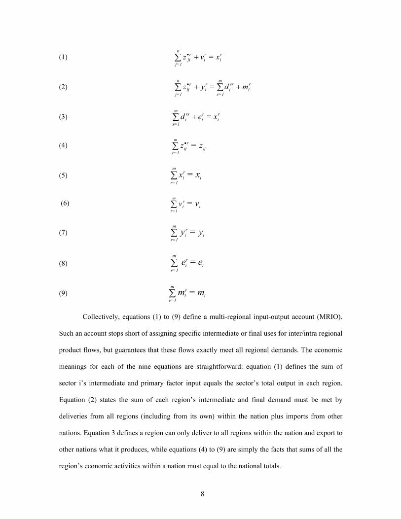
Collectively, equations (1) to (9) define a multi-regional input-output account (MRIO).

Such an account stops short of assigning specific intermediate or final uses for inter/intra regional

product flows, but guarantees that these flows exactly meet all regional demands. The economic

meanings for each of the nine equations are straightforward: equation (1) defines the sum of

sector i’s intermediate and primary factor input equals the sector’s total output in each region.

Equation (2) states the sum of each region’s intermediate and final demand must be met by

deliveries from all regions (including from its own) within the nation plus imports from other

nations. Equation 3 defines a region can only deliver to all regions within the nation and export to

other nations what it produces, while equations (4) to (9) are simply the facts that sums of all the

region’s economic activities within a nation must equal to the national totals.

9

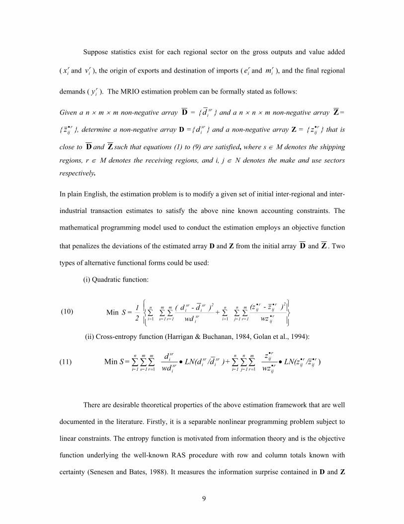
Suppose statistics exist for each regional sector on the gross outputs and value added

( rix and r

iv ), the origin of exports and destination of imports ( rie and r

im ), and the final regional

demands ( riy ). The MRIO estimation problem can be formally stated as follows:

Given a n × m × m non-negative array D = { srid } and a n × n × m non-negative array Z =

{ rijz • }, determine a non-negative array D ={ sr

id } and a non-negative array Z = { rijz • } that is

close to D and Z such that equations (1) to (9) are satisfied, where s ∈ M denotes the shipping

regions, r ∈ M denotes the receiving regions, and i, j ∈ N denotes the make and use sectors

respectively.

In plain English, the estimation problem is to modify a given set of initial inter-regional and inter-

industrial transaction estimates to satisfy the above nine known accounting constraints. The

mathematical programming model used to conduct the estimation employs an objective function

that penalizes the deviations of the estimated array D and Z from the initial array D and Z . Two

types of alternative functional forms could be used:

(i) Quadratic function:

(ii) Cross-entropy function (Harrigan & Buchanan, 1984, Golan et al., 1994):

(11) )Min11

rij

rijr

ij

rijm

r

n

j=1

n

=1i

sri

srisr

i

sri

m

r

m

=1s

n

=1iz/LN(z

wzz

+ )d/LN(d wdd

= S •••

•

==•• ∑∑∑∑∑∑

There are desirable theoretical properties of the above estimation framework that are well

documented in the literature. Firstly, it is a separable nonlinear programming problem subject to

linear constraints. The entropy function is motivated from information theory and is the objective

function underlying the well-known RAS procedure with row and column totals known with

certainty (Senesen and Bates, 1988). It measures the information surprise contained in D and Z

(10)

∑∑∑∑∑∑ •

••

==r

ij

2rij

rijm

=1r

n

j=1

n

isri

2sri

sri

m

=1r

m

=1s

n

i wz) z - (z

+ wd

)d -d (

21 = S

11Min

10

given the initial estimates D and Z . The quadratic penalty function is motivated by statistical

arguments. There are different statistical interpretations underlying the model by choices of

different reliability weights sriwd and r

ijwz • . When the weights are all equal to one, solution of

this model gives a constrained least square estimator. When the initial estimates are taken as the

weights, solution of the model gives a weighted constrained least square estimator, which is

identical to the Friedlander-solution, and a good approximation of the RAS solution. When those

weights are proportional to the variances of the initial estimates and the initial estimates are

statistically independent (the variance and covariance matrix of D and Z are diagonal), the

solution of the model yields best linear unbiased estimates of the true unknown matrix (Byron,

1978), which is identical to the Generalized Least Squares estimator if the weights are equal to

the variance of initial estimates (Stone, 1984, van der Ploeg, 1984). Furthermore, as noted by

Stone et al. (1942) and proven by Weale (1985), in cases where the error distributions of the

initial estimates are normal, the solution also satisfies the maximum likelihood criteria.

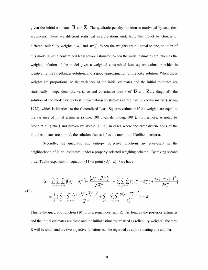
Secondly, the quadratic and entropy objective functions are equivalent in the

neighborhood of initial estimates, under a properly selected weighing scheme. By taking second

order Taylor expansion of equation (11) at point ( srid , r

ijz • ) we have

This is the quadratic function (10) plus a remainder term R. As long as the posterior estimates

and the initial estimates are close and the initial estimates are used as reliability weights4, the term

R will be small and the two objective functions can be regarded as approximating one another.

(12)

( ) ( )

R + z

)z (z +

d

) d-d ( 21

z2

zz+ zz +

d2d-d + d-d = S

rij

2rij

rij

m

1r=

n

1=j

n

isri

2sri

sri

m

1r=

m

1=s

n

i

m

rr

ij

rij

rijr

ijr

ij

n

=ij

n

1=i

m

r sri

sri

srisr

isri

m

1=s

n

=ii

}11

1

2

1

2

})(

){(}{

•

•−

•

==

=•

••••

=

∑∑∑∑∑∑

∑∑∑∑∑∑

=

−−

{

11

Thirdly, as proved by Harrigan (1990), in all but the trivial case, posterior estimates

derived from entropy or quadratic loss minimand will always better approximate the unknown,

true values than do the associated initial estimates. In this framework, information gain is

interpreted as the imposition of additional valid constraints or the narrowing of bounds on

existing constraints as long as the true but unknown values belong to the feasible solution set.

This is because adding valid constraints or further restricting the feasible set through the

narrowing of interval constraints cannot move the posterior estimates away from the true values,

unless the additional constraints are non-binding (have no information value). Although the

posterior estimates may not always be regarded as providing a "reasonable" approximation to the

true value5, they are always better than the initial estimates in the sense the former is closer to the

true value than the later, so long as the imposed constraints are true. In other words, the

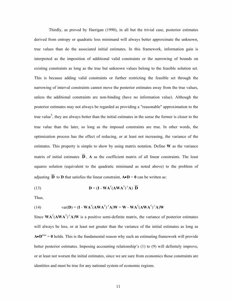
optimization process has the effect of reducing, or at least not increasing, the variance of the

estimates. This property is simple to show by using matrix notation. Define W as the variance

matrix of initial estimates D , A as the coefficient matrix of all linear constraints. The least

squares solution (equivalent to the quadratic minimand as noted above) to the problem of

adjusting D to D that satisfies the linear constraint, A•D = 0 can be written as:

(13) D = (I - WAT(AWAT)-1A) D

Thus,

(14) var(D) = (I - WAT(AWAT)-1A)W = W - WAT(AWAT)-1A)W

Since WAT(AWAT)-1A)W is a positive semi-definite matrix, the variance of posterior estimates

will always be less, or at least not greater than the variance of the initial estimates as long as

A•Dtrue = 0 holds. This is the fundamental reason why such an estimating framework will provide

better posterior estimates. Imposing accounting relationship’s (1) to (9) will definitely improve,

or at least not worsen the initial estimates, since we are sure from economics those constraints are

identities and must be true for any national system of economic regions.

12

Finally, the choice of weights in the objective function has very important impacts on the

estimation results. For instance, using the initial estimates as weights has the nice property that

each entry of the array is adjusted in proportion to its magnitude in order to satisfy the accounting

identities, and the variables cannot change sign and that large variables are adjusted more than

small variables. However, the adjustment relates directly to the size of the initial estimates

srid and r

ijz •, and does not force the unreliable initial estimates to absorb the bulk of the required

adjustment. Furthermore, only under the assumptions: (1) the initial estimates for different

elements in the array are statistically independent, and (2) each error variance is proportional to

the corresponding initial estimates, this commonly used weighing scheme (underlying RAS) can

obtain best unbiased estimates, while those assumptions may not hold in many cases. Fortunately,

the model is not restricted to use only a diagonal-weighing matrix such as the initial estimates.

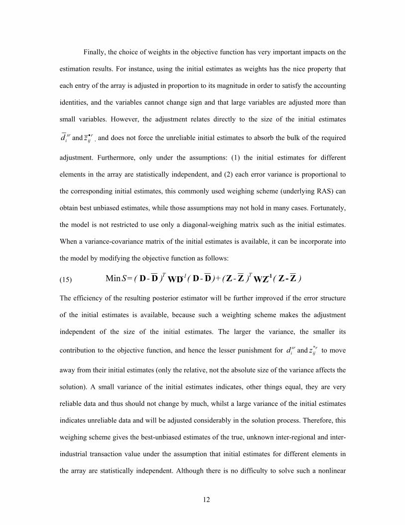
When a variance-covariance matrix of the initial estimates is available, it can be incorporate into

the model by modifying the objective function as follows:

(15) ) ( ) - ( + ) - ( ) - ( = S T-1T Z - ZWZZZDDWDDD -1Min

The efficiency of the resulting posterior estimator will be further improved if the error structure

of the initial estimates is available, because such a weighting scheme makes the adjustment

independent of the size of the initial estimates. The larger the variance, the smaller its

contribution to the objective function, and hence the lesser punishment for srid and r

ijz* to move

away from their initial estimates (only the relative, not the absolute size of the variance affects the

solution). A small variance of the initial estimates indicates, other things equal, they are very

reliable data and thus should not change by much, whilst a large variance of the initial estimates

indicates unreliable data and will be adjusted considerably in the solution process. Therefore, this

weighing scheme gives the best-unbiased estimates of the true, unknown inter-regional and inter-

industrial transaction value under the assumption that initial estimates for different elements in

the array are statistically independent. Although there is no difficulty to solve such a nonlinear

13

programming problem like this today, the major problem is lack of data to estimate the variance-

covariance matrix associate with the initial estimates.

Stone (1984) proposed to estimate the variance of rijz • as var( r

ijz • ) = ( rij

rij z •*θ )2, where

rij*θ is a subjectively determined reliability rating, expressing the percentage ratio of the standard

error to rijz • . Weale (1989) had used time series information on accounting discrepancies to infer

data reliability. The similar methods can be used to derive variances associated with those initial

estimates in our model.

Despite the difficulties in obtaining data for the best weighting scheme, advantages of

such a model in estimating interregional trade flows and interindustry transactions are still

obvious from an empirical perspective. Firstly, it is very flexible regarding the required know

information. For example, it allows for the possibility that the state total of output, value-added,

exports, imports and final demands are not known with certainty. In the real world, these regional

statistics typically have substantial gaps and inconstancies with the national total. Incorporating

associated terms similar to D and Z in the objective function to penalize solution deviations

from the initial estimates from statistical sources allows the estimation of those regional totals,

together with entries in the inter-regional delivery and inter-industrial transaction array. With the

use of upper and lower bounds, this fact can also be modeled by specifying ranges rather than

precise values for the linear constraints (1) - (3). In addition, the estimation of D or Z will be a

special case of the framework when only one set of additional data is available.

Secondly, it permits a wider variety and volume of information to be brought into the

estimation process. For example, the ability of introducing upper and/or lower bounds on those

regional totals is one of the flexibilities not offered by commonly used scaling procedures such as

RAS. The gradient of the entropy function tends to infinity as srid and r

ijz • → 0, and hence

14

restricts the value of the posterior estimates to nonnegative. This is a desirable property of

estimating inter-regional trade data.6

Thirdly, the weights in the objective function reflect the relative reliability of a given set

of initial estimates. The interpretation of the reliability weights is straightforward. Other things

equal, entries with higher reliability should be changed less than entries with a lower reliability.

The choice of those weights is also very flexible. They will use the best available information to

insure that reliable data in the initial estimates are not being modified by the optimization model

as much as unreliable data. In practice, such reliability weights can be put into a second array that

has the same dimension and structure as the initial estimates. The inverted variance-covariance

matrix of the initial estimates is statistically interpreted as the best index of the reliability for the

initial data.

Finally, solution of this estimation problem exactly provides the data needed to construct

a so-called multi-regional input-output (MRIO) model (Miller and Blair, 1985, Isard, et al. 1998).

This model was pioneered by professor Polenske and her associates at MIT in the 1970s

(Polenske, 1980), and is still widely used in regional economic impact analysis today.

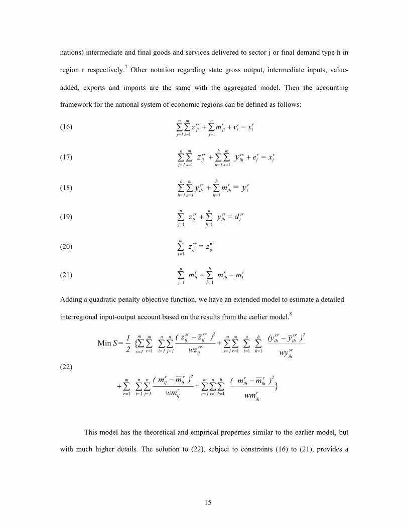
The above model could be easily extended to further allocate Z and D to distinguish

intermediate and final delivery of goods and services within a national system of economic

regions. The extended model will be similar in many aspects with the interregional accounting

framework proposed by Batten (1982) two decades ago. However, as we will show later in this

paper, it becomes more operational and provides better empirical estimation results on

interregional shipments because of the explicit incorporation of interregional trade flow

information into both the initial estimates and the accounting framework.

To demonstrate, denote srijz as intermediate inputs delivered from sector i in region s to

sector j in region r within a nation, and srihy as final goods and services delivered from sector i in

region s to type h final demand in region r. Further, denote rijm and r

ihm as imported (from other

15

nations) intermediate and final goods and services delivered to sector j or final demand type h in

region r respectively.7 Other notation regarding state gross output, intermediate inputs, value-

added, exports and imports are the same with the aggregated model. Then the accounting

framework for the national system of economic regions can be defined as follows:

(16) x =vmz ri

ri

n

j

rji

m

s

srji

n

1=j ++ ∑∑∑== 11

(17) x =e ri

ri

rsih

m

s

h

=1h

rsij

m

s

n

j=1y z

11++ ∑∑∑∑

==

(18) my ri

rih

h

=1h

srih

m

=1s

h

=1hy = ∑∑∑ +

(19) d = yz sri

srih

h

h

srij

n

j∑∑==

+11

(20) z =z r

ijsrij

m

s •

=∑

1

(21) m = mm ri

rih

h

h

rij

n

j∑∑==

+11

Adding a quadratic penalty objective function, we have an extended model to estimate a detailed

interregional input-output account based on the results from the earlier model.8

(22)

}

{

1 11

1111Min

rih

2rih

rih

n

i

h

h

m

=1rrij

2rij

rijn

j=1

n

=1i

m

r

srih

2srih

srih

h

h

n

i

m

r

m

=1ssrij

2srij

srijn

j=1

n

=1i

m

r

m

1s

wm

) mm ( +

wm)mm (

wy

)y(y +

wz) zz (

21 = S

−−+

−−

∑∑∑∑∑∑

∑∑∑∑∑∑∑∑

= ==

=====

This model has the theoretical and empirical properties similar to the earlier model, but

with much higher details. The solution to (22), subject to constraints (16) to (21), provides a

16

complete set of data for a so-called inter-regional input-output (IRIO) model with imports

endogenous (Miller and Blair, 1985, Isard, et al. 1998).

3. EMPIRICAL TEST OF THE MODEL AND EVALUATION MEASURES

The Testing Data Set

How does the model specified above perform when applied to data from the real world?

In order to evaluate the models’ performance, a benchmark data set from the real world is needed.

Because good interregional trade data are quite rare and very difficult to obtain in any country, a

natural place to find such data sets is existing global production and trade databases such as the

GTAP (Global Trade Analysis Project) database. For instance, version 4 GTAP database contains

detailed bilateral trade, transportation, and individual country’s input-output data covering 45

countries and 50 sectors (McDougall, Elbehri, and Trong, 1998). For our particular purpose,

version 4 GTAP database was first aggregated into a 4-region, 10-sector data set. Then three of

the four regions (the United States, European Union and Japan) were further aggregated into a

single open economy which engages in both interregional trade among its 3 internal regions and

international trade with the rest of the world. We will use this partitioned data set as the

benchmark for a hypothetical national economy, and attempt to use our model to replicate the

underlying inter-continental trade flows among Japan, EU and the United Sates as well as the

individual country’s input-output accounts.

Experiment Design

In the first experiment, we do this without use of the region-specific input-output

coefficients as the situation encountered in the real world, where only the national IO table is

available to economists (it is the three region’s weighted average in our experiment and are

defined as ( ) ( )rj

rjjjij

rij vxvxzz −×−=• )/( to make full use of the known information). Initial

estimates of interregional commodity flows are from the ‘true’ interregional trade data in the

17

GTAP database but was distorted by a normally distributed random error term with zero mean

and the size of standard deviation as large as 5 times the “true” trade data. The solution from the

model is compared with the benchmark data set for both the inter-regional shipment and inter-

sector transaction flows.

In the second experiment, we use the region-specific input-output coefficients as constant

in the model. We re-estimate the interregional shipment data as the first experiment, and compare

the model solution with the benchmark data set for the inter-regional trade data only.

In the third experiment, we assume the interregional shipment pattern is known with

certainty and we use the three region’s weighted average IO coefficients as initial estimates to

estimate the region-specific input-output accounts.

In the fourth experiment, Batten’s model was used to estimate the interregional shipment

and individual region’s IO flows. In the fifth to the seventh experiments, experiments 1-3 were

repeated by using the extended model. Solutions from both models are compared with the “true”

interregional trade and inter-sector IO flow data in the aggregated GTAP data set. The

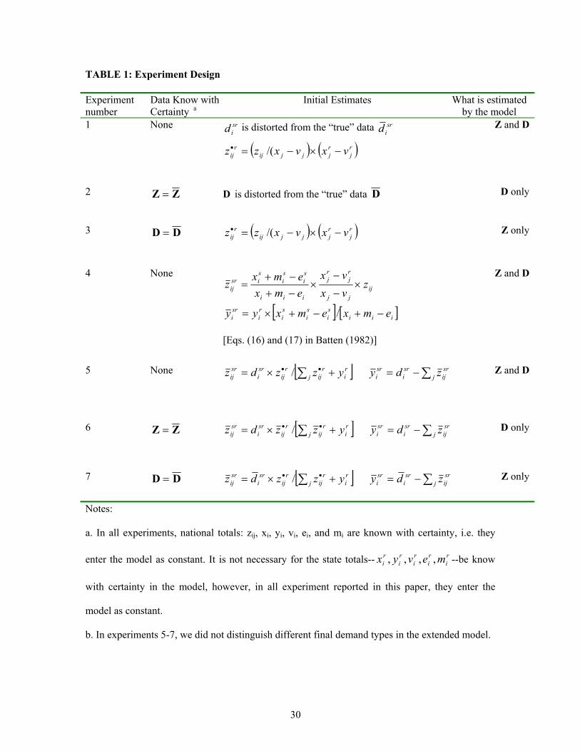
assumptions, initial estimates and expected model solution are summarized in table 1.

(Insert Table 1 here) Measures to Evaluate Test Results

Each experiment produces a different set of estimates, and it is desirable to know how much each

set of estimates differs from the true, known data. However, it is difficult to use a single measure

to compare the estimated results. Since there are so many dimensions in the model solution sets, a

particular set of estimates may score well on one region or commodity but badly on others. It is

meaningful to use several measures to gain more insight on the model performance in different

experiments. Generally speaking, it is the proportionate errors and not the absolute errors that

matter; therefore, the "mean absolute percentage error" with respect to the true data will be

calculated for different commodity and regional aggregations. Consider the following aggregate

index measure for intra/inter-regional trade flows:

18

(23) sr

i

m

r

m

=1s

n

=1i

sri

sri

m

r

m

=1s

n

=1iD

d

|dd | 100 = MAPE

∑∑∑

∑∑∑

=

=−•

1

1

Alternating the removal of summations over i, s, and r in equation (23) produces MAPE estimates

on shipments by commodities, shipping regions, and receiving regions respectively. For regional

intermediate transactions, the aggregate MAPE index is defined as:

(24) r

ij

m

r

n

j=1

n

=1i

m

r

rij

rij

n

j=1

n

=1iZ

z

|z - z | 100 = MAPE

•

=

=

••

∑∑∑

∑∑∑•

1

1

Alternating the removal of summations over i, j, and r in equation (24) produces MAPE estimates

on intermediate transactions by inputs, using sectors, and regions respectively. The model and all

test experiments are implemented in GAMS and the complete GAMS program and related data

set are available from the authors upon request.

Test Results

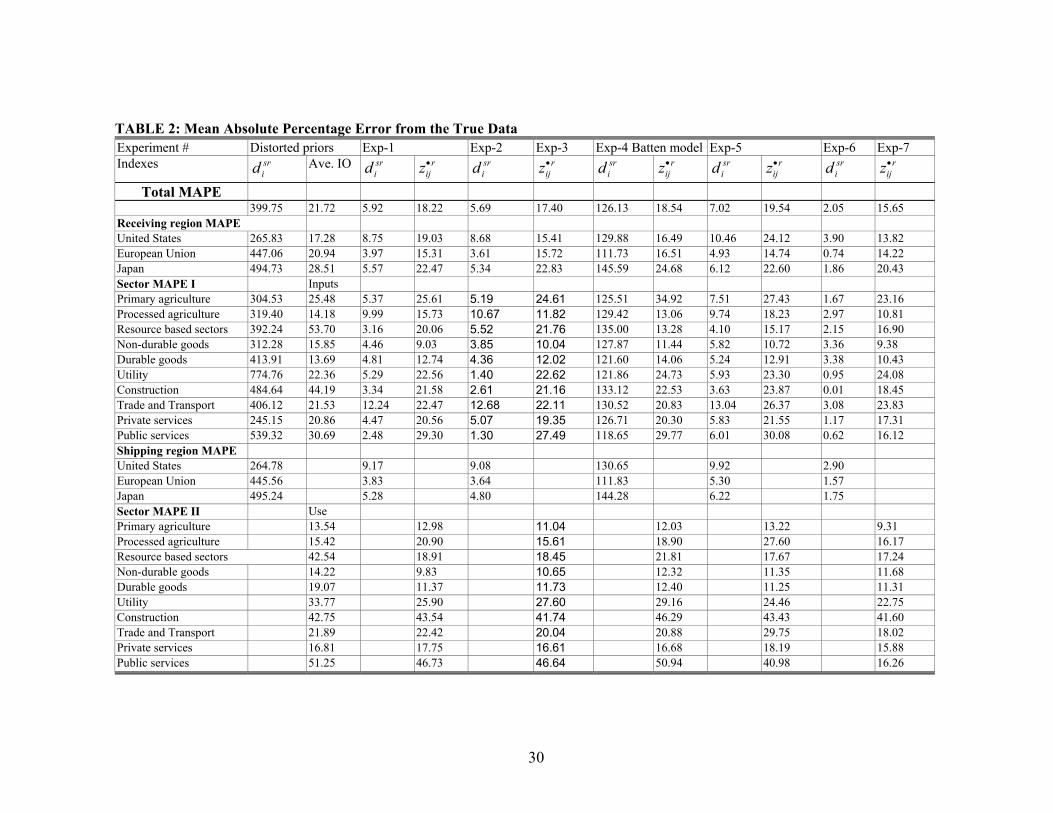
Table 2 summarizes all the eight measurement indexes from the seven experiments listed

in Table 1. The accuracy of the estimates is judged by their closeness to the true interregional

trade and individual region’s input–output flows aggregated from the GTAP database.

(Insert Table 2 here)

Generally speaking, the model has remarkable capacity to rediscover the true

interregional trade flows from the highly distorted data. The estimated shipment data are very

close to the true data, as judged by the eight MAPE measurements, in all testing experiments

except the Batten model. Most of the mean absolute percentage errors are about 4-7 percent of the

true data value, which implies the model has great potential in the application of estimating

interregional trade flows. In contrast, recovering the individual region’s input-output flows from

weighted average national values only obtained limited success, indicating national IO

19

coefficients in detailed sectors may be the best place to start in building regional IO accounts if

there is no additional prior information on regional technology or cost structure available.9

Comparing estimates from different test experiments, there are several interesting

observations. First, when there is no additional information that could be incorporated into the

estimation framework, a more detailed model may not perform better than a simpler model.

Comparing results from Exp-1 and Exp-5, the more sophisticated extended model actually brings

less accurate estimates overall because of increasing numbers of unknown variables without

additional known data. However, as results in Experiments 2, 3, 6, and 7 show, the estimation

accuracy does improve by a more detailed model when more useful data become available.

Second, the marginal accuracy gained from actual individual regional IO flows is significant in

estimating interregional trade flows using the extended model, but very small in the aggregate

version. In contrast, the marginal value of accurate interregional shipment data is rather small in

estimating individual regional IO coefficients under both versions of the model. Finally, Batten’s

model performed poorly in interregional shipment estimation, but obtained similar estimates on

individual regional IO flows as our model, providing further evidence that there may be no high

dependency between individual regional IO coefficients and interregional trade flows. However,

this is not a firm conclusion because the particular data set used to test the model in this paper

may be part of the problem. Since the United States, EU and Japan are all large economies, their

intermediate demands are largely met by their own production. Therefore, the correlation between

individual inter-industrial flow and inter-regional shipments may be particularly low.

The extended model only provides better estimates of interregional shipments when

regional IO data are available, so the aggregate version of the model specified in this paper may

be the best practitioner’s tool in estimating interregional trade flows because of the lack of sub-

national IO data in the real world. It demands less statistical information and has a smaller model

dimension, which facilitates the implementation and computation process.10

20

4. IMPLICATIONS FOR APPLYING THE MODEL

Results in the previous section offer some guidance for applying the framework outlined

in this paper to real world statistics. It was found that initial estimates of regional commodity

trade flows based on survey data with very high statistical variability are highly preferable (in the

experiments) to a widely used non-survey approach for producing initial estimates.11 This finding

holds promise for opportunities to use other survey data to recover unobserved regional economic

accounts. It was also found that solving an aggregate account (e.g., a MRIO or MR-SAM) as an

intermediate step is at least as accurate (in the experiments) as producing a direct solution to an

extended account (e.g., IRIO or IR-SAM) when superior data unique to the later are not widely

available. This finding is useful when working with regional economic accounts of considerable

sector and region details. Results also support the product mix approach, whereby the most

feasible sector detail for regional gross output estimates are used to derive weighted average

national technical coefficients for more aggregated regional sectors.

Statistical systems vary by nation and no one-size fits all rules exist that tell us how to

seamlessly employ every data-system to best advantage.12 However, there are general guidelines

for implementing the optimization framework presented in this paper to a large dimension multi-

regional account. To facilitate discussions of implementation, we assume that a detailed national

account always exists and regional sector statistics are also available in a variety of details. Then

the implementation process may be classified into three broad phases as discussed below.

Develop Independent Estimates for Major Components of a Multi-regional Account

It has been stressed as far back as Wilson (1970) that information used to produce

parameters and initial estimates of a regional economic system should be estimated

independently. While this produces unbalanced initial accounts, it avoids introducing spurious

information that can lead to biased estimates (McDougall, 1999). A useful approach is to partition

the multi-regional account into components that coincide or are related to known statistical

survey series published regularly in the nation under study.

21

For the multi-regional IO account outlined in equations (1) to (9), the major components

are gross regional output ( rix ), final demand ( r

iy ), primary factor payments ( riv ), international

trade ( rie and r

im ), inter-industry transactions ( rijz • ) and inter/intra-regional trade flows ( sr

id ). In

many cases, data for several of these components are available from a single major statistical

survey series—for example, in the United States rix and r

iv are available from an Economic

Census conducted every five years. Other components, for example riy , may themselves require

multiple disparate data sources to compile. While the strategic groupings may differ by country, it

is likely that for large dimension (N × M) multi-regional accounts, primary data for individual

regional sectors become sparse.

When the best available data are not consistent to the model structure, it may be

necessary to restructure the adding up requirements in the model to accommodate the data. For

example, in equation’s (2) and (3) of our model, the accounting identities require data for

international exports ( rie ) and imports ( r

im ) on an origin of movement and destination of use

basis respectively. However, in many countries such as the United Sates, port of entry/exit data

are far more reliable. Therefore, different formulation of the corresponding accounting identities

should be used.

For certain elements of the multi-regional account, very often only a purely theoretical

inference is available to produce informed guesses about the initial estimates. A common

example is the information about service trade flows within and between regions. In using a

theory-based alternative to data, a case must be made for a prevailing empirical model that

calibrates the unobserved activities to some other statistics or available survey data.

Determine Model Dimensions Based on Maximum Concordance among Different Components

In compiling different components of the multi-regional account, the volume and nature

of data available for each component can greatly vary. Detailed and survey based data may be

22

obtained on, for example, gross regional output and incomes, but survey data on the inter/intra-

regional trade flows of this output may be far less detailed. Inter-industry transactions may only

be available at the national level, and international trade data may be very detailed, but based on a

different product classification system. The notion of conservatism, both in the information

theoretic sense and in terms of computational burden, should be the primary guiding principal in

reconciling this information.

Robinson et al. (2001) interpret conservatism by the rule of using ‘only, and all’

information in the estimation problem. Considering this rule in the present context, the fact that a

component such as gross regional outputs are available from highly detailed and reliable statistics

suggests all this information should be used. However, if the associated intra/inter-regional trade

flow account has more general product aggregations than the output account, it appears that one is

faced with an ‘only or all’ decision. Although the specific situation often guides the approach one

takes, it is worth noting that there are usually many opportunities to introduce all information

available into the estimation process.

In practice, conserving on computational burden may also become an issue. When

employing a more general estimation framework such as the model presented in this paper, the

use of iterative techniques that diminish computational burden may not be readily available.13

Both computer hardware and software available to the researchers may become binding in many

such instances. For example, access to special solvers or greater programming finesse becomes a

more prominent issue when computational burdens grow tremendously as model dimension

increase. In addition, while conventional personal computers have improved dramatically, limits

on current 32-bit operating systems to manage sufficient memory on PC’s may become a binding

constraint for very large models. Solutions to these issues can become expensive.

Add Additional Constraints to Use All Available Information

The greatest opportunities to use all relevant information are in the form of additional

binding linear constraints, beyond the adding up and consistency requirements, on any selected

23

groups of variables in the aggregate or extended model. Information deemed ‘superior’ and that is

related to any group of elements in either the aggregate or extended accounts is a candidate for a

linear constraint. Since both interregional and multi-regional economic accounts are

comprehensive and detailed, there are many opportunities to introduce such constraints. A few

general guidelines are notable.

Both the aggregate and extended accounts describe flows of payments and products in the

form of a matrix with known adding-up and consistency requirements. Any information used to

formulate new constraints—either equality or inequality linear constraints—can greatly diminish

the feasible solution set of the calibration procedure. However, new constraints that are non-

binding add no information to the problem, but do increase the computational burdens.

Where and how information is used to formulate constraints depends on many factors.

For example, the U.S. Government has published state measures of farm productivity that include

estimates of purchased farm inputs by state for broad input categories. A pro-rated version of this

data could form the basis for additional linear constraints for agricultural sector I-O flows in the

model. Other restrictions could be designed to replicate certain highly reliable economic statistics

that can be formed by special groupings of certain flow statistics contained in the account being

estimated. Although such information must be carefully compiled, their incorporation in the form

of constraints will improve the estimation accuracy greatly.

5. CONCLUSIONS AND DIRECTION FOR FUTURE RESEARCH

This study constructed a mathematical programming model to estimate interregional

trade patterns and input-output accounts based on an interregional accounting framework and

initial estimates of interregional shipments in a national system of economic regions. The model

is quite flexible in its data requirements and has desirable theoretical and empirical properties. An

empirical test of the model using a 4-region, 10-sector example aggregated from a global trade

database shows that the model performs remarkably well in discovering the true patterns of

24

interregional trade from highly distorted initial estimates on interregional shipments. It shows the

model may have great potential in the estimation and reconciliation of interregional trade flow

data, which often are the most elusive data to assemble. In addition, solutions from the aggregated

model exactly provides the data needed for a MRIO model and the solution from the extended

model exactly provide the data needed for an IRIO model. This will greatly reduce the data

processing burden in such analysis. Therefore, application of the model will further facilitate

quantitative economic analysis in regional sciences.

Lessons from the experiments in this study shaped our view on approaches for applying

the model to real data from a particular nation’s statistics. A logical conclusion is that widely

available and disparate survey data on the economy, including commodity flows data and

incomplete geographic data, can effectively be used to substantially narrow the margins for error

in obtaining feasible solutions to interregional input-output systems. It is also evident that data on

region-to-region commodity flows represent a limiting factor in determining the optimal sector

dimensions to be solved in the modeling framework.

However, there are important questions not yet answered by the current study. First, test

results from the data set aggregated from GTAP also show that our model’s ability to improve the

IO transaction estimates of individual regions from national averages may be limited. Continuing

research on the real underlying causes and means of improvement are needed to further enhance

the model’s capacity as an estimating and reconciliation tool in building interregional production

and trade accounts. Second, the relative importance of regional sector output, value-added,

exports, imports and final demand as model input in the accuracy of a model solution is also not

analyzed, and could be addressed with minor changes of the current model. Third, the approach

employed in this study draws primarily from regional science and constrained matrix balancing

literatures. How insights from economic geography theory can help define a bounded solution

needs to be explored. Finally, the robustness of the model’s performance should be further tested

using other data sets.

25

Footnotes:

1. Wilson (1970) had suggested an entropy maximizing solution for a model which integrated

gravity models and multi-regional input-output equations as constraints to estimate inter-regional

commodity flows. However, his work did not clearly incorporate a complete system of national

and regional input-output accounts as did in Batten (1982).

2. Using Monte Carlo simulation, Robinson, Cattaneo and El-said (2001) shows that when

updating column coefficients of a Social Accounting Matrix (SAM) is the major concern, the

cross entropy method appears superior, while if the focus is on the flows in the SAM, then the

two methods are very close with the RAS performing slightly better.

3. The variables srid and r

ijz • have no counterparts in Batten’s framework, reflecting important

departures in the present approach.

4. The quadratic functional form has a numerical advantage in implementing the model. It is

easier to solve than the entropy function in very large models because they can use software

specifically designed for quadratic programming.

5. The minimand objective function reflects the principle that the 'distance' between the posterior

and initial estimates should be minimized. What we would like is to minimize the 'distance'

between the posterior estimates and the unknown true values. This 'distance' cannot be measured,

but a good estimation procedure should have a desirable influence on it.

6. Zeros can become non-zeros and vice versa under a quadratic penalty function. However, a

side effect for the cross entropy function is that if there are too many zeros in the initial estimates,

the whole problem may become infeasible.

7. The assignment of an intermediate (j) or final demand use (h) of international imports has no

counterpart in Batten’s notation since he makes no such assignments. Either approach is valid and

would be dictated by the data available.

8. By incorporated the 6 accounting identities that the sum of all regions in the nation should

equals their national totals defined in equations (4-9), the model could be solved independently

without use of the earlier model, however, the dimension and data requirements of the model will

be much larger than the aggregated model.

9. Following the product mix method outlined in Miller & Blair (1985), initial estimates of IO

coefficients for each of the 10 aggregated industries are unique for each region. They are

weighted averages of the 3-region detailed (50-industry) IO coefficients where the weights are the

gross regional outputs of the relevant detailed industries. Experiment results show that a “product

mix” approach improves the accuracy of the true regional IO flow estimates compared to an

26

approach that directly uses the 3-region average IO coefficients, although the differences are

small in our particular model aggregation.

10. The aggregate model only has N(NM+M2+5M) variables and N(3M+N+5) constraints, while

the extended model has (N2M + NHM)(M+1) variables and N(M2+NM+N+5) constraints. This is

a much larger model, having NM2(N-1) + NM(HM-5) more variables and MN(M+N-3)

additional constraints.

11. A random normal distortion of the ‘true’ trade data by an average of 400-percent was

produced in the previous section to simulate a well designed but poorly sampled transportation

survey of annual commodity flows.

12. Comprehensive studies by West (1990) and Lahr (2001) consider how to identify and use

superior data in a regional accounting system context.

13. For example, by allowing both regional technical coefficients and intra/inter-regional flows to

adjust, the optimal solution to the cross-entropy or quadratic formulations in section 2 must be

jointly solved.

27

References

Bartholdy, Kasper. 1991. "A Generalization of the Friedlander Algorithm for Balancing of National Accounts Matrices," Computer Science in Economics and Management 2, 163-174. Batten, David F. 1982. " The Interregional Linkages Between National and Regional Input-Output Models," International Regional Science Review, 7, 53-67. Batten, David F. and D. Martellato. 1985. “Classical Versus Modern Approaches to Interregional Input-Output Analysis,” Annals of Regional Science, 19, 1-15. Boomsma, Piet and Jan Oosterhaven. 1992. “ A Double-entry Method for the Construction of Bi-regional Input-Output Tables,” Journal of Regional Sciences, 32(3), 269-284. Bregman, L. M. 1967. "Proof of the Convergence of Sheleikhovskii's method for a problem with transportation constraints," USSR Computational Mathematics and Mathematical Physics, 1(1), 191-204. Byron, R. P. 1978. "The Estimation of Large Social Account Matrix," Journal of Royal Statistical Society, A, 141(Part 3), 359-367. Byron, R. P., P.J. Crossman, J.E. Hurley and S.C. Smith. 1993 "Balancing Hierarchial regional Accounting Matrices," Paper presented to the International Conference in memory of Sir Richard Stone, National Accounts, Economic Analysis and Social Statistics, Siena, Italy. Golan, Amos, George Judge, and Sherman Robinson. 1994. "Recovering Information From Incomplete or Partial Multisectoral Economic Data," The Review of Economics and Statistics, LXXVI(3), 541-549. Harrigan, Frank J. 1990. "The Reconciliation of Inconsistent Economic Data: the Information Gain," Economic System Research, 2(1), 17-25. Harrigan, Frank J. and Iain Buchanan. 1984. "A Quadratic Programming Approach to Input-Output Estimation and Simulation." Journal of Regional Science, 24(3), 339-358. Isard, Walter, Iwan Azis, Matthew P. Drennan, Ronald E. Miller, Sidney Saltzman, and Erik Thorbecke, eds., 1998. Methods of Interregional and Regional Analysis. New York: Ashgate Publishing Company. Jensen, Rodney C. 1990. “Construction and Use of Regional Input-output Models: Progress and Prospects” International Regional Science Review, 13(1 & 2), 9-25. Lahr, M.L. 2001. “A strategy for producing hybrid regional input-output tables,” in Lahr, Michael, and Erik Dietzenbacher (eds.), Input-Output Analysis: Frontiers and Extensions. Basingstoke, U.K: Palgrave, pp. 211-242. McDougall, R.A., A. Elbehri, and T.P. Truong. 1998. “Global Trade Assistance and Protection: The GTAP 4 database,” Center for Global Trade Analysis, Purdue University.

28

McDougall, R. A. 1999. “Entropy Theory and RAS are Friends,” Paper presented at the 5th conference of Global Economic Analysis, Copenhagen, Denmark. Miller, R. E. and P.D. Blair. 1985 Input-Output Analysis: Foundations and Extensions. Englewood Cliffs, New Jersey: Prentice Hall. Mohr, M., W. H. Crown and K. R. Polenske. 1987. "A Linear Programming Approach to Solving Infeasible RAS Problems." Journal of Regional Sciences, 27(4), 587-603. Nagurney, A. and A.G. Robinson. 1989. "Equilibration Operators for the Solution of Constrained Matrix Problems," Working Paper, OR 196-89, Operations Research Center, MIT. Polenske, Karen R. 1980. The U.S. Multiregional Input-Output Accounts and Model. Lexington, Mass.: Lexington Books. Robinson, Sherman, Andrea Cattaneo and Moataz El-Said. 2001. “ Updating and Estimating a Social Accounting Matrix Using Cross Entropy Methods” Economic System Research, 13(1), 47-64. Senesen, G. and J. M. Bates. 1988. "Some Experiments with Methods of Adjusting Unbalanced Data Matrices." Journal of the Royal Statistical Society, A. 151(Part 3), 473-490. Stone, R. 1984. "Balancing the national accounts. The adjustment of initial estimates: a neglected stage in measurement," in A. Ingham and A.M. Ulph (eds.), Demand, Equilibrium and Trade. London: Macmillan. Stone, R., J. M. Bates and M. Bacharach. 1963. A programme for Growth, Vol. 3 Input-Output Relationship 1954-1966, London: Chapman and Hall. Stone, R., D.G. Champernowne and J.E. Meade. 1942. "The precision of national income estimates." Review of Economic Studies, 9(2), 110-125. Trendle, Bernard. 1999. “Implementing A Multi-regional Input-Output Model – The Case of Queensland,” Economic Analysis & Policy, Special Edition, 17-27. van der Ploeg, F. 1982. "Reliability and the adjustment of Sequences of Large Economic Accounting Matrices," Journal of the Royal Statistical Society, A. 145, 169-194. van der Ploeg, F. 1984. "General Least Squares Methods for Balancing Large Systems and tables of National Accounts," Review of Public Data Use, 12, 17-33. van der Ploeg, F. 1988. " Balancing Large Systems of national Accounts," Computer Science in Economics and Management 1, 31-39. Weale, M. R. 1985. "Testing Linear Hypotheses on National Account data," Review of Economics and Statistics, 67, 685-689. Weale, M. R. 1989. “Asymptotic maximum-likelihood estimation of national income and expenditure,” Cambridge, mimeo.

29

West, G. R. 1990. “Regional Trade Estimation: A Hybrid Approach” International Regional Science Review, 13,103-118. Wilson, A. G. 1970. “Inter-regional Commodity Flows: Entropy Maximizing Approaches,” Geographical Analysis, 2, 255-282. Zenios, A. Stavros, Arne Drud and John M. Mulvey. 1989. " Balancing Large Social Accounting Matrices with Nonlinear Network Programming." NETWORKS, 19, 569-585.

30

TABLE 1: Experiment Design

Experiment number

Data Know with Certainty a

Initial Estimates What is estimated by the model

1 None srid is distorted from the “true” data sr

id

( ) ( )rj

rjjjij

rij vxvxzz −×−=• /(

Z and D

2 ZZ = D is distorted from the “true” data D D only

3 DD = ( ) ( )rj

rjjjij

rij vxvxzz −×−=• /( Z only

4 None

[ ] [ ]iiisi

si

si

ri

sri

ijjj

rj

rj

iii

si

si

sisr

ij

emxemxyy

zvxvx

emxemx

z

−+−+×=

×−

−×

−+−+

=

/

[Eqs. (16) and (17) in Batten (1982)]

Z and D

5 None [ ] ∑∑ −=+×= ••j

srij

sri

sri

rij

rij

rij

sri

srij zdyyzzdz /

Z and D

6 ZZ = [ ] ∑∑ −=+×= ••j

srij

sri

sri

rij

rij

rij

sri

srij zdyyzzdz /

D only

7 DD = [ ] ∑∑ −=+×= ••j

srij

sri

sri

rij

rij

rij

sri

srij zdyyzzdz /

Z only

Notes:

a. In all experiments, national totals: zij, xi, yi, vi, ei, and mi are known with certainty, i.e. they

enter the model as constant. It is not necessary for the state totals-- ri

ri

ri

ri

ri mevyx ,,,, --be know

with certainty in the model, however, in all experiment reported in this paper, they enter the

model as constant.

b. In experiments 5-7, we did not distinguish different final demand types in the extended model.

30

TABLE 2: Mean Absolute Percentage Error from the True Data Experiment # Distorted priors Exp-1 Exp-2 Exp-3 Exp-4 Batten model Exp-5 Exp-6 Exp-7 Indexes sr

id Ave. IO srid r

ijz• srid r

ijz• srid r

ijz• srid r

ijz• srid r

ijz•

Total MAPE 399.75 21.72 5.92 18.22 5.69 17.40 126.13 18.54 7.02 19.54 2.05 15.65 Receiving region MAPE United States 265.83 17.28 8.75 19.03 8.68 15.41 129.88 16.49 10.46 24.12 3.90 13.82 European Union 447.06 20.94 3.97 15.31 3.61 15.72 111.73 16.51 4.93 14.74 0.74 14.22 Japan 494.73 28.51 5.57 22.47 5.34 22.83 145.59 24.68 6.12 22.60 1.86 20.43 Sector MAPE I Inputs Primary agriculture 304.53 25.48 5.37 25.61 5.19 24.61 125.51 34.92 7.51 27.43 1.67 23.16 Processed agriculture 319.40 14.18 9.99 15.73 10.67 11.82 129.42 13.06 9.74 18.23 2.97 10.81 Resource based sectors 392.24 53.70 3.16 20.06 5.52 21.76 135.00 13.28 4.10 15.17 2.15 16.90 Non-durable goods 312.28 15.85 4.46 9.03 3.85 10.04 127.87 11.44 5.82 10.72 3.36 9.38 Durable goods 413.91 13.69 4.81 12.74 4.36 12.02 121.60 14.06 5.24 12.91 3.38 10.43 Utility 774.76 22.36 5.29 22.56 1.40 22.62 121.86 24.73 5.93 23.30 0.95 24.08 Construction 484.64 44.19 3.34 21.58 2.61 21.16 133.12 22.53 3.63 23.87 0.01 18.45 Trade and Transport 406.12 21.53 12.24 22.47 12.68 22.11 130.52 20.83 13.04 26.37 3.08 23.83 Private services 245.15 20.86 4.47 20.56 5.07 19.35 126.71 20.30 5.83 21.55 1.17 17.31 Public services 539.32 30.69 2.48 29.30 1.30 27.49 118.65 29.77 6.01 30.08 0.62 16.12 Shipping region MAPE United States 264.78 9.17 9.08 130.65 9.92 2.90 European Union 445.56 3.83 3.64 111.83 5.30 1.57 Japan 495.24 5.28 4.80 144.28 6.22 1.75 Sector MAPE II Use Primary agriculture 13.54 12.98 11.04 12.03 13.22 9.31 Processed agriculture 15.42 20.90 15.61 18.90 27.60 16.17 Resource based sectors 42.54 18.91 18.45 21.81 17.67 17.24 Non-durable goods 14.22 9.83 10.65 12.32 11.35 11.68 Durable goods 19.07 11.37 11.73 12.40 11.25 11.31 Utility 33.77 25.90 27.60 29.16 24.46 22.75 Construction 42.75 43.54 41.74 46.29 43.43 41.60 Trade and Transport 21.89 22.42 20.04 20.88 29.75 18.02 Private services 16.81 17.75 16.61 16.68 18.19 15.88 Public services 51.25 46.73 46.64 50.94 40.98 16.26

30

RLuz L:\JRSresub.doc July 1, 2004 2:14 PM