A Computational Approach to Wav e Motion in One and Two Dimensions

1. Introduction

Computational physics has evolved into an equally valid approach to exploring the laws of nature,augmenting the more familiar experimental and theoretical approaches. It affords access to physicalregimes hitherto unapproachable. This inaccessibility may be due to limitations of temporal acuity, if therelevant time scales are too short as in explosive reactions, or too long as in climate modeling or the evolu-tion of the Universe. There may be physical limitations due to hostile environmental conditions which pre-vents direct observation as, for example, in the core of the Sun. Many problems exhibit several limitationssuch as in a supernova. These computational laboratories are meant to introduce students at the highschool level to the computational approach to problem solving. The intent is not to create computationalphysicists nor to teach computer programming. Therefore the emphasis will not be on creating the pro-grams (although their algorithms will be discussed) but on the underlying concepts. Whenever possible, thederivations have used only algebraic or geometrical arguments, to allow the greatest possible dissemination.Where possible, the relationship to the Calculus is included for those few high schools in which it is taught.

The techniques used in computational physics often appear cumbersome to the student used to thetraditional problem solving technique of finding exact analytical solutions. The objections often centeraround the complaint that the answers are only approximate. This overlooks the many lev els of approxima-tions built into the ‘‘exact’’ analytical solutions. The physical equations (often called ‘‘laws’’) are them-selves approximate descriptions of the physical world. There are scale approximations which depend uponthe requirements of the problem -- different approximations are required for sub-atomic, molecular, macro-scopic, or universal scales. Spatial approximations are often employed as simplifying assumptions reduc-ing the complexity from three dimensions to two dimensions, or only one dimension. Forces having no sig-nificant influence are ignored, such friction or gravity, which are always present but unimportant for manyapplications. This list could continue, but the point is that ‘‘approximate solutions’’ hav e always beenappropriate, assuming that some care was exercised in the approximating. Often these approximations areself evident: sub-atomic physics is not the best way to describe galaxy mergers, for example. In order tomake responsible choices concerning which approximations should be made, some general knowledge andexperience with the possibilities and possible results is required. It is the same with computational physics,which has its own levels of approximation and different techniques (and resulting complications) of prob-lem solution. An operational definition of problem solution will be used here. ‘‘A problem is consideredsolved if, at any desired time, the required quantities ( e.g. position or velocity) are known to within a rea-sonable tolerance.’’

Computational physics is not simply plugging values into an analytic solution to get quick numbers.(That is the purpose of pocket calculators.) Rather, one starts with the basic equations and assumptions rel-evant to the problem to be solved. The computer is then used to advance these equations in space or time(or both) starting from a specified state, called the initial conditions. This is often performed as a series ofsmall steps or iterations. As a simple example of the computational approach, consider a simple harmonicoscillator.

2. Simple Harmonic motion

Figure 2.1 should be familiar to anyone with a knowledge of physics. It consists of a mass mattached to a massless spring. The spring is attached to an immovable wall at the right. The mass is con-strained (as in a trough) to one dimensional horizontal motion, without friction. (Note the approximations!)The equilibrium position is x0. It is assumed that the spring obeys Hooke’s Law

F = −k (x − x0), (2.1)

where F is the force exerted by the spring on the mass and k is the spring constant, expressing the spring’sstiffness. Equation (2.1) is simply a mathematically elegant way of stating what in English can becomequite cumbersome: ‘‘when the length of a spring is changed by being stretched or compressed beyond its

-2-

Figure 2.1 This problemhas intrigued physics studentsfor generations. A massattached to a spring isallowed to slide back andforth on a frictionlesssurface. The equilibriumspring length is x0. 666666666666666

666666666666666666666666666

m

x0

equilibrium (relaxed) length, a force is exerted by the spring to resist this change in length. This restoringforce is linearly proportional to the change in length. For example, the force doubles if the change in lengthdoubles. ’’ Newton’s 2nd law is needed to relate the acceleration of the mass to the force produced by thespring. This law states that the force exerted on an object is directly proportional to its observed accelera-tion, or

F = m a, 2.2

where m, the constant of proportionality, is the inertial mass. Combining equations (2.1) and (2.2) pro-duces

ma = −k (x − x0). (2.3)

This is often called the equation of simple harmonic motion, because the motion this equation describesconsists of a periodic sinusoidal movement that has a single frequency, which is

f =1

2π √ k

m(2.4)

One computational approach to solving this equation might begin by dividing time into discrete inter-vals of length ∆ t. This introduces a standard notation which is used throughout this paper: that a change(usually small) in some quantity q from the one value q1 to another value q2 is

∆ q = q2 − q1. (2.5)

Please take careful note of the order of subtraction. This follows the generally accepted convention of‘‘new’’ minus ‘‘old’’, which may give rise to negative changes. Now the equation to be solved (here, eqn2.3) must be converted into a form compatible with modern digital computers. This may involve express-ing other quantities in addition to time in terms of small changes as well. This process is called a dis-cretization of the equation.

First consider the general definition of velocity:

v =∆(position)

∆(time). (2.6)

Equation (2.6) states that velocity is a change in position divided by that change in time over which thischange in position occurred. Likewise, acceleration is

a =∆(velocity)

∆(time). (2.7)

The form of this discretization should be familiar to those with some knowledge of the Calculus. Forexample the definition of the derivative is

df (x)

dx=

lim

∆x− > 0

f (x + ∆x) − f (x)

∆x. (2.8)

Equation (2.3) now becomes

∆v

∆t= −

k

m(x − x0) (2.9)

The change in velocity may be written as

-3-

∆v = vn+1 − vn, (2.10)

which is the difference between the velocity at the new time level and the velocity at the old. The numberof timesteps or iterations taken so far is given by the superscript which, in this standard notation, does notimply an involution (exponentiation). The use of ‘‘n’’ rather than some specific number implies the equa-tion is general and valid for any timestep. An expression for the new or updated velocity may now bederived from eqn (2.9):

vn+1 = vn −k

m(xn − x0)∆t 2.11a

Likewise, the updated position is

xn+1 = xn +(vn + vn+1)

2∆t 2.11b

(The astute reader will have noted that in eqn. (2.11b) the velocity used to advance the position in time wasthe average of the velocity at the beginning of the timestep, vn, and the velocity at the end of the timestep,vn+1.)

The procedure is to first select a small timestep ∆t and then, beginning with the initial conditions,step forward in time by finding successive values for position and velocity from eqns (2.11). It should benoted that such a solution no longer consists of a continuum of positions or velocities, but of values foundonly at specific points in time determined by the size of the timestep.

From the discretization of the equations, one would expect the accuracy of this computational solu-tion to increase as the timestep decreases. This can be verified using a pocket calculator. Howev er, evenafter only a couple of oscillations it should become clear that the answer diverges, that is, the oscillationsgrow larger with each repetition, regardless of how small the timestep is made (tables 1 and 2, figure 2.2).This behavior, called numerical instability, is undesirable.

0 5 10

-4

-2

0

2

4

x-di

spla

cem

ent

Figure 2.2 This shows results from two different timesteps using the unstable numerical algorithm given by eqns. (2.11) when used for the simple harmonic oscillator shown in figure 2.1.

The initial conditions are: x0 = 0, x 0 = 1, and v

0 = 0.

Results using two different timesteps are displayed. Circles are the results using a timestep of ∆ t = 0.25, squares are the results using a timestep of ∆ t = 0.5. Note the increasing amplitude with each oscillation, betraying the unstable nature of the algorithm.

The problem is buried within equation (2.11a). The new velocity is is computed with a constantacceleration: the acceleration at the beginning of the timestep. This ignores the change in acceleration asthe position changes from xn to xn+1 during the timestep ∆t. Thus the acceleration is always over-estimated in the velocity calculation. Each time the mass slows and reverses direction, at the left and right

-4-

ends of its motion, the deceleration is underestimated by using accelerations calculated only from ‘‘old’’values. This is a systematic error, and in computational physics systematic errors generally accumulate tounfortunate effect.

A way to correct this is to advance the position using velocities computed halfway through the timestep. That is, equations (2.11) now become

vn+ /12 = vn− /1

2 +k

m(xn − x0) ∆ t (2.12a)

xn+1 = xn + vn+ /12 ∆t. (2.12b)

The resulting scheme is known as a leapfrog scheme because of the computational grid pattern (figure2.3). Numerical grids such as the one shown in figure 2.3, in which some quantities are computed only atcertain grid points and other quantities are computed only at points betwixt, are call staggered grids.

tn

tn+1

tn+2

tn+3

tn+3/2

tn+1/2

tn+5/2

Figure 2.3 In a leapfrog scheme, some quantities are calculated at on integral points in time (∆t, 2∆t, 3∆t, ...), while other quantities are calculated at points in between ∆ t, ∆ t, ∆ t, ...). The name of this family of numerical schemes is derived from this pattern.

1_2

52_3

2_

position (x)

velocity (v)

Time axis

One disadvantage of leapfrog type schemes is the cumbersome initial condition requirement: knowl-edge of the unknown velocity, v− /1

2 , at the at time t = −∆t /2, would be required. In practice, the value attime t = 0 is used instead. This introduces a small starting error, the magnitude of which is dependent uponthe size of the timestep. However, this error does not grow as the calculation progresses. (The technicalterm for such small errors is starting glitch.) The stability of this scheme can be easily demonstrated on apocket calculator. (Table 3, figure 2.4. Note that the use of vn− /1

2 = 0 causes the magnitude of the resultingoscillations to be approximately 1.03 rather than 1.00 as would be expected for the given parameters. Notealso that this error does not grow.)

3. Isolated mass between two springs

This problem is a simple extension of the isolated mass on a spring problem. It will prove usefullater in constructing a model of a stretched string.

a. Theory

First consider the geometry of figure 3.1. A mass m is suspended between two vertical attachmentsby two identical massless springs. Gravity is neglected. Each spring exerts a force on the mass. Recallthat force is a vector quantity, so that both magnitude and direction are important. At the equilibrium posi-tion shown in figure 3.1, the two forces are equal in magnitude, and collinear, with opposite directions. Ifleft undisturbed, the mass will remain in this position.

-5-

0 5 10-1.5

-1

-.5

0

.5

1

1.5x-

disp

lace

men

t Figure 2.4 This shows results from the stable leapfrog algorithm given by eqns (2.12). The initial conditions are: x0= 0, x0 = 1, and v−1/2 = 0. The timestep is ∆ t = 0.5.

Note that the error introduced by using v −1/2 = 0 for the velocityat t=−1/2 causes the magnitude of the amplitude to be about 3% larger than the expected 1.0. This starting error does not grow.

m

666666666666666666666666

666666666666666666666666666666666666

l0l

0

S1

S2

F1

F2

Figure 3.1 This shows a mass suspended between two vertical posts by two massless springs. The springs pull on the weight with sufficient force to that gravity may be neglected, that is, as shown here at equilibrium, there is no appreciable vertical displacement.

Now consider a vertical displacement of the mass by a small amount as shown in figure 3.2. Assumethat this displacement is much smaller than the length of the two springs, l0. Now the forces exerted on themass by the two springs are no longer collinear, causing the vector nature of a force to become apparent.

-6-

Figure 3.2 This shows the same mass and springs as in figure 3.1, but with a small vertical displacement (greatly exaggerated here). This vertical displacement y is much smaller than the length of either spring, l .

666666666666666666666666

666666666666666666666666666666666666

l0l

0

S1

S2

my

θ θ

F2

F2,y

F2,x

F1

F1,y

F1,x

0

Recall that a vector is a quantity enjoying both magnitude and direction. Vectors will be representated by abold typeface in equations. To determine the resulting motion, these forces must be resolved into their hor-izontal and vertical vector components, that is, the components parallel to the x-axis and the y-axis, resp.In this way the force created by spring S1 may be expressed as

F1 = −F1 cos(θ ) x − F1 sin(θ ) y, 3.1a

and the force created by spring S2 may be expressed as

F2 = F2 cos(θ ) x − F2 sin(θ ) y. 3.1b

Here x is a unit vector pointing in the positive x-direction and y is a unit vector pointing in the positive y-direction. The total force acting on the mass is the vector sum of these two forces, or

F = F1 + F2 = (F2 − F1) cos(θ ) x − (F1 + F2) sin(θ ) y. (3.2)

When the springs are identical, that is, Fs = F1 = F2 (where Fs is the magnitude of the force exerted byone of the springs on the mass), the horizontal components are equal in magnitude, but opposite in direc-tion, thus canceling. This leaves only a vertical component

F = −2Fs sin(θ ) y. (3.3)

Next, it must be determined by how much each spring is stretched further (if at all) by the small verti-cal displacement. The length of each spring is now

l′ = √ l20 + y2 = l0√ 1 +

y

l0

2

, (3.4)

-7-

found by using the theory of Pythagoras, which equates the square of the length of the hypotenuse of aright-angled triangle to the sum of the squares of the lengths of its two legs. If the vertical displacement yis small compared to l0, then

√ 1 +

y

l0

2

≈ 1. (3.5)

Therefore any additional stretching of the springs due to small vertical displacements of the mass is negligi-ble. Because there is no appreciable change in length of the strings, then application of Hooke’s law, eqn.(2.1), implies no appreciable change in the magnitude of the forces exerted on the mass by the springs.That is, Fs is constant. Using

sin(θ ) =y

√ l20 + y2

=y

l0 √ 1 + (y/l0)2≈

y

l0, (3.6)

in which equation (3.5) has been used to make this approximation, the restoring force felt by the mass is

F = −2 Fs

l0y. (3.7)

It should be stressed that the restoring force arises not from any increase in the magnitude of the forces act-ing on the mass, but purely from the changes in the directions of these forces. That is, the restoring forcearises from the vector nature of a force. Understanding this point is crucial for the remaining discussion.The equation of motion for the mass becomes

may = −2 Fs

l0y (3.8)

This is again the form of the familiar equation of simple harmonic motion, eqn. (2.3). This motion has asingle frequency

f =1

2π √ 2 Fs

ml0(3.9)

b. Numerical Example

The string program was written to simulate the behavior of a continuous vibrating string. Neverthe-less, by running it using its coarsest possible representation of the string, it can also be used to simulate thebehavior of a single mass suspended by two springs. First, one selects difference scheme number 2, with 1point mass, from the graphical user interface (gui), figure 3.3.

It may prove useful to realize that the total length is, by construction, unity so the spacing betweenmasses (which is obviously the length of the springs, l0) is determined by the number of masses requested.Thus, with only one mass, l0 = 1⁄2. Exploration of the relationship between the various parameters may nowproceed. It should be noted that only the tension and mass affect the frequency of the resulting motion. Inparticular it should be noted that the frequency is independent of the initial displacement and initial veloc-ity. This may be demonstrated by plotting of position vs. time and velocity vs. time for various choices ofinitial conditions.

It is suggested that the various user-adjustable parameters be chosen such that

2Fs

m l0= 1. (3.10)

With this simplification, eqn (3.8) becomes

ay = −y. (3.11)

Using this choice of parameters, verify that given an initial displacement in position (a0) or an initial veloc-ity (v0) of 0.01, oscillations are produced in both position and velocity (as a function of time) having equalamplitudes but differing phase. Phase is the difference between a particular point or stage of an oscillationrelative to a standard position such as an extremum. Or in other words, the oscillations produced by eitheran initial displacement (but no initial velocity) or by an initial velocity (but no initial displacement) obtaintheir maxima and minima at different times, but are otherwise the same. This is illustrated by figure 3.4afor the specific initial conditions of a0 = 0. 01 and v0 = 0. 0, (example A) and figure 3.4b for the specific

-8-

Figure 3.3 This is an example of a typical setup for a single mass. The leapfrog method discussed in the text has clearly been selected.

initial conditions of a0 = 0. 0 and v0 = 0. 01 (example B). Now measure the resulting amplitudes of theoscillations in position and velocity when the initial position displacement is doubled (2a0) and halved(1⁄2a0). It should be noted that the resulting oscillation amplitudes double and halve, respectively. This is aconsequence of the linearity of this problem: the response is directly proportional to the input.

Another consequence of linearity is that when the initial conditions consist of a combination of twosimpler initial conditions, the resulting behavior is the sum of the behaviors of these two components. Forexample, combine the above two examples A and B to produce the initial conditions a0 = 0. 01; v0 = 01.The amplitude of the resulting oscillations is not 0. 02, but approximately 0.013, because the solutionsmust be added in phase, as illustrated by figure 3.5 using position displacement oscillations. In figure 3.5,the transverse displacement as a function of time is plotted at various points for the two examples A and B.Also plotted is the transverse displacement as a function of time resulting from the combination of the ini-tial conditions of examples A and B ( a0 = 0. 01; v0 = 0. 01). At each point in time, the resulting

-9-

0 5 10-1.5

-1

-.5

0

.5

1

1.5

-1.5

-1

-.5

0

.5

1

1.5po

sitio

n (y

)

0 5 10-1.5

-1

-.5

0

.5

1

1.5

-1.5

-1

-.5

0

.5

1

1.5

posi

tion

(y)

Figure 3.4 Here are two examples showing the sinusoidal behaviour of small oscillations of a mass suspended between two springs. In 3.4A (left) the initial conditions consist of a small displacement in position but no ititial velocity, while in 3.4B (right) the initial conditions consist of a small initial velocity but no position displacement. The same behaviour results from either. The two oscillations differ only in phase

displacement is the sum of the displacements of A and B. Because A and B are not in phase, the maximumdisplacement is not the simple sum of the maxima of A and B. The frequency is, of course, the same. Theconstruction of a similar diagram for the velocity is left to the reader.

4. A Chain of Masses

The example of an isolated mass between two springs from the previous section will now beextended to a one dimensional chain of masses and springs.

a. Theory

Now consider several masses and springs tethered together as in figure 4.1. It is assumed that thespacings are equal and that any incremental transverse displacement, yi − yi−1, is small relative to this spac-ing. Subscripts are used to indicate the spatial relationships among individual objects or measurements.For example, mi refers to any individual mass, mi−1 is the next mass on its left, and mi+1 is the next masson its right. If the vertical displacement is represented by y, then yi , yi−1, and yi+1 are the vertical displace-ments of the three previously mentioned masses, respectively. The use of i indicates that the relationshipbeing discussed is general and applies to any mass. If a specific mass is desired, it would be indicated byits specific ordinal number: m1 would indicate the first mass, for example. Note that in a long chain, theabsolute displacement of mass j is the sum of all the individual incremental displacements from the first

-10-

line, squares). The resulting oscillation has the same frequency as either of the two individual oscillations, but differing amplitude and phase.

Figure 3.5 This is an example of linearity. Here, the solid line (stars) results from initial conditions consisting of both a positional displacement and an initial velocity. The resulting oscillations are simply the sum of the oscillations due to either problem in isolation, that is, initial conditions consisting only of a displacement, but no initial velocity (dotted line, squares) and initial conditions consisting only of an initial velocity, but no displacement (dashed

0 5 10-1.5

-1

-.5

0

.5

1

1.5

-1.5

-1

-.5

0

.5

1

1.5

posi

tion

(y)

X(0) = 1.0; V(0) = 0.0X(0) = 0.0; V(0) = 1.0= +

∆x

Figure 4.1. This shows a chain of identical masses and springs. The masses of the springs are negligible, and they exert sufficient force on the masses to prevent any appreciable sagging of the chain. This allows gravity to be neglected. The length of each spring at equilibrium (spacing between masses) is everywhere the same: ∆ x.

mass:

y j − y0 =j

i=1Σ yi − yi−1. 4.1

Thus the absolute displacement can be relatively large.

Now the forces affecting the ith mass, mi , will be constructed using figure 4.2. Figure 4.2 depicts ashort segment from fig. 4.1 with a transverse displacement. As with the problem of a single mass sus-pended between two springs of section 3, the horizontal force components will cancel, assuming smallincremental displacements, leaving only a vertical component

F = Fs(sin(θ l) − sin(θ r )), (4.2)

where Fs is the magnitude of the force each spring exerts on the individual masses, θ l is the angle thespring to the left of the mass makes with respect to the horizontal, and θ r is the angle the spring to the rightof the mass makes with respect to the horizontal. From figure 4.2 it is clear that

-11-

one directed towards mass mi+1 making an angle θr with the horizontal. The horizontal componentsof the net force cancel, leaving only a net vertical component.

directed towards mass mi−1 making an angle θl with the horizontal, and than the spacing of the masses, ∆ x. Two forces act on mass m

i : one

here for illustrative purposes and is assumed to be much smaller vertical displacement. This displacement is exaggerated

shown in figure 4.1 which has undergone a small of the chain of identical masses and springs

Figure 4.2. This shows a small section

i+1

i

θR

i-1

θL

sin(θ l) =yi − yi−1

√ (∆x)2 + (yi − yi−1)2≈

yi − yi−1

∆x(4.3)

and

sin(θ r ) =yi+1 − yi

√ (∆x)2 + (yi+1 − yi)2≈

yi+1 − yi

∆x, (4.4)

using the approximation of eqn. (3.4). Thus the acceleration on the ith mass becomes

ai =Fs

mi

yi+1 − yi

∆x−

yi − yi−1

∆x

. (4.5)

A numerical solution may now be constructed using eqns (2.12):

vn+ /12

i = vn− /12

i +Fs

mi ∆x(yn

i−1 − 2 yni + yn

i+1) ∆ t (4.6a)

and

yn+1i = yn

i + vn+ /12

i ∆t. (4.6b)

(The relationship with the single mass of section 3 can be made apparent by holding masses mi−1 and mi+1

stationary, and setting their offsets yi−1 and yi+1 to zero. Equation (4.6a) then becomes

vn+ /12

i = vn− /12

i + 2Fs

mi ∆xyn

i ∆ t. (4.6a’)

This is recognizable as eqn. (3.8) ).

Obviously, the initial conditions must specify the starting displacements and velocities for each mass.To complete one timestep, eqns (4.6) must be computed N times for N masses. The advantages of fastcomputers quickly become evident when considering a problem involving thousands of individual masses.

Most readers will have noticed a problem using eqns (4.6): information for the non-existent 0th massis required to update m1, as well as information for the non-existent (N+1)th mass in order to update the lastor N th mass. This additional information, called the boundary conditions (for obvious reasons), must alsobe supplied, defining the positions and velocities of the missing points. For fixed ends (as shown in theillustrations here) these conditions are particularly simple: no motion. These conditions are usually calledreflecting, or hard wall, boundary conditions.

b. Numerical Examples

As with the single mass, we use the LCSE string numerical laboratory and difference method 2, butnow with 2 masses, figure 4.3. As you may recall, one mass produced only one type of motion. The up-down-up-down motion observed in section 2.b. There was nothing else the single mass could do. A moreprecise way of saying this is that there existed only one degree of freedom, and there was only one mode ofvibration. Now, with two masses, there are two degrees of freedom which will produce two fundamentalmodes of vibration.

-12-

Figure 4.3 This shows the LCSE string program in a typical setup for two masses using the leapfrog method described in the text.

The analysis of these two modes begins with equation (4.5) to provide the acceleration for m1:

a1 =Fs

m1

y2 − y1

∆x−

y1 − y0

∆x

. (4.7)

Using the assumption of reflecting boundary conditions in which the end points are held stationary ( that is,y0, y3 = 0) this becomes

a1 =Fs

m1

y2 − 2 y1

∆x

. (4.8a)

Likewise, the acceleration for m2 is

-13-

a2 =Fs

m2

y1 − 2 y2

∆x

. (4.8b)

These are an example of a coupled set of equations: the motion of m1 depends upon the position of m2, andconversely.

666666666666666666

@@@@@@

@@@@@@@@@

a. In this mode, both masses move in phase. Each mass has the same vertical displacement and both have the same velocities and accelerations.

b. In this mode, both masses are out of phase. The vertical displacements of each mass have the same magnitudes, but opposite signs.

666666666666666666

@@@@@@

@@@@@@@@@

Figure 4.4. With two individual masses, two distinct vibratory modes are possible.

666666666666666666

666666666666666

When the masses are identical, there exist two special configurations which can be easily analyzed bymost people. The first mode is a motion in which the two masses move in phase (figure 4.4a and figure 4.5,left column). To see this, begin with identical displacements (y1 = y2 ) and zero velocities. Then eqns.(4.8) become

a1 = −

Fs

m ∆x

y1 (4.9a)

and

a2 = −

Fs

m ∆x

y2 (4.9b)

Thus each mass undergoes simple harmonic motion. They begin in phase, and remain in phase since theirindividual accelerations are always the same. Using eqn. (2.4), this motion has a frequency of

f =1

2π √ Fs

m ∆x. (4.10)

The subscripts on the mass m have been dropped because we have assumed That they are identical.

In the second mode the two masses are out of phase, shown in figure 4.4b and figure 4.5, middle col-umn. This may be initialized using zero initial velocities with displacements which are opposite in sign,but equal in magnitude (y1 = −y2 ). Now eqns. (4.8) become

a1 = −

3 Fs

m ∆x

y1 (4.11a)

and

a2 = −

3 Fs

m ∆x

y2. (4.11b)

Again, each mass undergoes simple harmonic motion. In this mode, they begin out of phase, and remain sosince their individual accelerations are always the same. This motion has a frequency of

-14-

Time

Mode(j=2)[ Mode(j=1) +Mode(j=1)]Mode(j=1)

Figure 4.5 These are snapshots of the oscillations of two masses given three different initial conditions. The snapshots are taken at equal times and at uniform intervals, with time increasing from top to bottom. The left and middle columns are the j=1 and j=2 resonate modes, resp. Note the different oscillation frequencies. The initial amplitude of mode j=1 is twice that of mode j=2. The initial conditions for the right column is the sum of these two modes. Note the subsequent behaviour is at any one time the sum of the two modes at that time.

f =1

2π √ 3 Fs

m ∆x. (4.12)

(A similar analysis utilizing velocities rather than displacements is left as a relaxing little exercise for thereader.)

It should be noted that the two different modes have different frequencies: the frequency of the inphase mode being lower than that of the out of phase mode. Furthermore, these two modes are

-15-

independent. Initial conditions which are a linear combination of these two modes (as illustrated in figure4.5) results in motion which is the sum of the two individual oscillations. This is easily verified by thestring lab by the interested reader. Any desired initial conditions may be expressed as a linear combinationof these two modes. Figure 4.6 shows how the initial conditions in which only one of the masses has a dis-placement may be constructed.

Figure 4.6 Any initial conditions may be created from a linear combination of the two normal modes of vibration. This shows that the initial conditions consisting of only one of the two masses having a positional offset is the result of a simple sum of the symmetric and antisymmetric modes.

6666666666

66666666

66666666

6666666666

}∆y

-∆y

∆y

66666666

66666666 2∆y

An analytical analysis like the above for more than two masses is hopelessly beyond the scope of thistext. However, a qualitative approach follows.

Each allowed mode of vibration, called a normal mode, corresponds to some integral number of half sinewaves corresponding to the equilibrium length of the chain of masses and springs. This integral number ofhalf sine wav es, j, is the mode number of the vibration. It will be shown, but mercifully not derived, thatfor N particles, there exist only j = 1, 2, 3, . . . , N distinct modes. Assuming the separation of the masses(that is, the length of the springs), ∆x is uniform, the initial position of the ith particle for the jth normalmode may be determined by evaluating

yi = A j sin

π j xi

∆x (N + 1)

, (4.13)

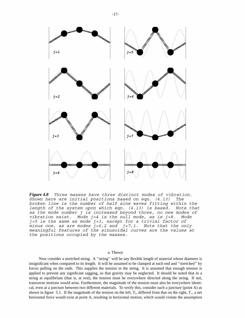
where xi is the x-location of the ith mass, N is the number of masses, A j is the (small but arbitrary) ampli-tude of the jth mode, and j is the mode number, j = 1, 2, . . . , N . The resulting patterns for two and threemasses are shown in figures 4.7 and 4.8. The broken lines are the curves, f (x), resulting from an equationsimilar to eqn. (4.13) in which the discrete locations xi are replaced by a continuous variable, x:

f (x) = A j sin

π j x

∆x (N + 1)

. (4.14)

The only physically meaningful features of these curves are the values at the positions occupied by themasses! Because this has confused so many people, this statement will be repeated: The only physicallymeaningful features of these curves are the values at the positions occupied by the masses! Thesepositions are indicated by large dots, rendering them easily visible to the older reader. Some peoplebecome confused by such diagrams, giving the continuous curves more physical meaning than exists. Forthese systems of masses, there is nothing special about the extrema, or the nodes of these curves. This con-fusion undoubtedly arises from the fact that the system consists of a small number of discrete masses, not acontinuous system. Therefore, the extrema and nodes are not necessarily occupied by masses as somewould assert. Figure 4.7 shows the displacements for the two modes allowed by two masses, and figure4.8 shows the displacements for the three modes allowed by three masses. It is clear from this that there is

-16-

Figure 4.7 This clearly shows that a system made up of a discrete number of particles has a limited number of unique modes of vibration j: j=1,2,...,N where N is the number of particles. Increasing j beyond N produces solutions which have already been depicted. For two masses, as shown here, there are two modes, j=1, j=2. Mode j=3 is the null mode (not meaningful), j=4 is the same as j=2 (except for a trivial minus sign) as are modes j=5, and j=1. Mode j=6 is again the null mode. The broken line is from eqn. (4.13). Note that the only meaningful features of these cures are the values at the positions occupied by the masses.

j=3

j=4

j=5j=2

j=6

j=1

an upper limit to the frequency (or equivalently, a lower limit on wav elength) which can be uniquely repre-sented. This limit is reached when the displacements exhibit an alternating up-down-up-down pattern.Such a limit will exist regardless of the number of masses chosen, but of course at differing wav elengths fordiffering numbers of masses, assuming the total length of the chain is the same in all cases. The longerwavelengths, however are easily represented as the number of masses increases. Figure 4.9 shows the twolowest modes (j = 1 and j = 2) for nine, 10, and 11 masses. By comparing figure 4.9 with figures 4.7 and4.8, it is clear that as the number of masses increase, the behaviour approaches that of a continuous stringfor long wav elength modes. That is, the discrete nature of the model does not appreciably affect themotion.

5. A Stretched String

-17-

j=1

j=2

j=3

j=4

j=5

j=6

j=7

j=8

Figure 4.8 Three masses have three distinct modes of vibration. Shown here are initial positions based on eqn. (4.13) The broken line is the number of half sine waves fitting within the length of the system upon which eqn. (4.13) is based. Note that as the mode number j is increased beyond three, no new modes of vibration exist. Mode j=4 is the null mode, as is j=8. Mode j=5 is the same as mode j=3, except for a trivial factor of minus one, as are modes j=6,2 and j=7,1. Note that the only meaningful features of the sinusoidal curves are the values at the positions occupied by the masses.

a. Theory

Now consider a stretched string. A ‘‘string’’ will be any flexible length of material whose diameter isinsignificant when compared to its length. It will be assumed to be clamped at each end and ‘‘stretched’’ byforces pulling on the ends. This supplies the tension in the string. It is assumed that enough tension isapplied to prevent any significant sagging, so that gravity may be neglected. It should be noted that in astring at equilibrium (that is, at rest), the tension must be everywhere directed along the string. If not,transverse motions would arise. Furthermore, the magnitude of the tension must also be everywhere identi-cal, even at a juncture between two different materials. To verify this, consider such a juncture (point A) asshown in figure 5.1. If the magnitude of the tension on the left, Tl , differed from that on the right, Tr , a nethorizontal force would exist at point A, resulting in horizontal motion, which would violate the assumption

-18-

9 MASSES

10 MASSES

11 MASSES

Figure 4.9 Displayed here are the lowest two modes (j=1 on the left and j=2 on the right) for strings of 9, 10, and 11 masses. Long wavelength vibratory modes are easily represented by even a relatively small number of discrete masses. The discrete nature of the model becomes apparent for modes whose wavelengths are comparable to the spacing of the masses.

that the string was at equilibrium.

For sufficiently long samples, almost any solid substance could be made into a string, thus its soledefining parameter is its linear density. Because some readers may not be comfortable with the concept oflinear density, a little further explanation may be in order. This terminology comes from the most generaldefinition of density, that is

-19-

Figure 5.1 At equilibrium, the tension within a string must be uniform, even when the string is a composite. Here a string is composed of two different materials joined at point A. If the magnitude of the tension on the left, Tl, differed from that on the right, T

r, a net horizontal force would exist at point A, resulting in

horizontal motion, violating the assumption that the string was at equilibrium.

A

TL TR

density =mass

volume, (5.1)

where volume is determined by the dimensions of the problem. In three dimensions, the volume element,or unit volume, is the unit of length, cubed. Examples are: cubic feet, cubic centimeters, and cubic meters.Thus, in three dimensions, density, or volume density, enjoys such familiar units as slugs† per cubic foot,grams per cubic centimeter, kilograms per cubic meter, etc.

However, when solving some specific problem, any special geometrical properties of that problemare used to simplify its solution. This simplification often includes reducing the dimensions to two (say fora flat plate, or motion confined to a table top ) or to one (as in this case of a string). In two dimensions, thevolume element is length squared, producing surface densities such as slugs per square foot (at the Earth’ssurface, force is often used in the English system to produce pounds per square foot), kilograms per squaremeter, grams per square centimeter. In one dimension density becomes a linear density, examples of whichare slugs per foot (or pounds per foot if you really insist), kilograms per meter, or grams per centimeter.Thus eqn (5.1) is really

density =mass

length(number of dimensions) , (5.2)

There may be also some confusion with the concept of density and the physical diameter of the wire.It is obvious that when given two wires of the same composition, the wire with the greater linear densitywill have a larger diameter, but this is not necessarily the case when the composition of the two wires differ,as for example, steel and plastic. It may prove useful to compare the resulting diameters of wires madefrom various materials with the same linear densities (but differing volume densities). For example twosteel wires whose linear densities differ by a factor of two, or a steel write and a plastic rope.) Next con-sider the forces on a short segment or element of the string as in figure 5.2. The mass of the string elementis

mi = λ ∆l ≈ λ∆xi (5.3)

The directions of the forces at each end of this element are tangent to the string at these points. In generalthese directions are not exactly parallel, giving rise to a net vertical force

Ts (sin(θ l) − sin(θ r )). (5.4)

Thus if the string is considered to be constructed of a large number of small segments, the tangents may beapproximated by drawing lines connecting the centers of adjacent segments, and if each segment is consid-ered to be a mass λ∆x concentrated at the center of that segment connected to each other by springs, themodel from the previous section may be used. Substituting eqn. (5.3) for mi in eqn. (4.4) produces

ai =Fs

λ1

∆x

yi+1 − yi

(∆x)−

yi − yi−1

(∆x)

. (5.5)

† If you do not know what a slug is, then shame on you.

-20-

That a string could be modeled in this manner should not really be surprising. At the molecular level, this isvery close to what the problem really is: a set of mass concentrations (atoms or molecules) held together byrestoring forces (electrostatic forces), but at a much smaller scale than can be realistically computed.

element and an angle θ r at the right edge. Both of these angles are small, so that ∆l ≅ ∆x. The vertical scale is magnified in this illustration.

the length of this element is much smaller that the total length of the

parallel, making an angle θl with respect to the horizontal at the left edge of the tangent to the string at these points. In general these directions are not exactly

string. The directions of the forces acting on each end of this element are

Figure 5.2 This shows a string element ∆l. It is assumed that

∆l

∆x

θR

θL

Readers familiar with the calculus will recognize that1

∆x

yi+1 − yi

(∆x)−

yi − yi−1

(∆x)

from the right-hand

side of eqn. (5.5) is really the second derivative of y with respect to x, in the limit that ∆x → 0. Using thedefinition of acceleration:

a =∂2 y

∂2t, (5.6)

eqn. (5.5) becomes

∂2 y

∂2t=

Fs

λ∂2 y

∂2 x. (5.7)

This is known as the wave equation, a dynamical relationship appearing in many seemingly unrelated cir-cumstances, from wav es on strings to light. For light, the wav e equation reads

∂2 y

∂2t=

c2

η2

∂2 y

∂2 x, (5.8)

where η is the index of refraction of the medium through which the light is traveling, and c is the speed oflight in vacuum. Therefore, the same numerical algorithm developed to simulate wav es in strings will sim-ulate plane light wav es if the identification

c

η= √ Fs

λ(5.9)

is made.

b. Dissipation

There is one addition necessary to complete this numerical string model. After some considerationof the figures in section 4 above, it is apparent that there are allowed some very ‘‘unstring-like’’ modes ofvibration: particularly a very high frequency (short wav elength) up-down motion shown in figure 5.3. Thisis known as a grid oscillation since it occurs at the highest resolution of the numerical grid. At the atomiclevel, the atoms do vibrate in modes such as this, but not in a manner which is coordinated across the entirediameter of the string. Such small-scale motions are eventually dissipated as heat. In the computationalmodel as it now stands, no such dissipation exists, and any such short wav elength (high frequency) vibra-tions are allowed to remain, which would violate the assumption that the string model was smooth. Themodel for a smooth string must therefore not allow any vibrations to occur with wav elengths comparable to

-21-

Figure 5.3 Here is an example an allowed up−down motion or grid oscillation. This is the highest frequency (shortest wavelength) allowed on the numerical grid. In actual objects, such vibrations would occur at the molecular scale and would be dissipated as heat. Because the computational resolution cannot extend to the molecular level, additional numerical dissipation must be added to avoid grid oscillations.

the size of the string element or discretization. Therefore dissipation is added to the computation to dampthese unwanted vibratory modes.

To add dissipation to the model one must first realize that not only are the positions oscillating in thisup-down manner, but the velocities must be oscillating as well to produce such displacements. Thus if agiven mass, mi is in a region undergoing such an oscillation, its velocity will be different than its nearestneighbors. However, many modes are allowable, as was demonstrated in the last section. In the very longwavelength modes, which are well described by this string model, the velocity of mi is very close to theav erage of its neighbors. This suggests that the long wav elength signals could be preserved while dampingthe short wav elength oscillations if the velocities used in eqn (4.6b), vn+ /1

2

i , are replaced by a blend of thatvelocity and a velocity found from some interpolation using its neighboring masses:

vi ′ = (1 − f )vn+ /12

i + f vi , (5.10)

where f is the fractional weighting, 0 ≤ f ≤ 1, and vi , is the interpolated velocity.

++++

8888

vi

^’

vi

^

vi

vi-1 v

i+1

Figure 5.4 Here are shown velocities in part of a string of masses for which the motion has two components. One is a long wavelength component, shown as a dotted line. The other component is the grid oscillation from figure 5.3. Two methods are offered for damping the short wavelength component while leaving the long wavelength component relatively unscathed. One procedure blends the velocity at each point with the value obtained by a simple average of the two nearest neighbors (dashed line). This is method 3 in the LCSE lab. The other procedure blends the velocity at each point with a values obtained by fitting a curve to the four neared neighbors ( dot−dash line). This is offered as method 4 in the LCSE lab.

This interpolated velocity, vi , may be determined by a number of procedures. Tw o are offered in theLCSE string laboratory, figure 5.4. First, a simple average (straight-line interpolation) of the two nearestneighbors:

v =vi−1 + vi+1

2. (5.11)

This is incorporated into method 3 in the LCSE string laboratory. The second uses a smooth curve, here acubic polynomial,

g(x) = A + Bx + Cx2 + Dx3, (5.12)

-22-

which passes through the four nearest points, and evaluating that curve at x = xi to obtain v′i as shown infigure 5.4. This is incorporated into method 4 in the LCSE string laboratory.

For those who really must know, v′i may be found in the following procedure. The point masses areuniformly spaced, so the symmetry of the problem suggests using weighted averages of the neighboringpoint masses taken in symmetrical pairs:

vi = α (vn+ /12

i−1 + vn+ /12

i+1 ) + β (vn+ /12

i−2 + vn+ /12

i+2 ). (5.13)

Some tedious algebra will reveal that α = 2/3 and β = −1/6. This may be verified in the following manner.If eqn (5.13) holds for the special cases: vi = xi , vi = x2

i , and vi = x3i , then it must work for all linear com-

binations of them, and hence for all polynomials of the desired form, eqn (5.12). Choose xi as the centralmass, setting xi = 0. Using a spacing ∆x of 1 gives

xi±1 = ±1 (5.14a)

and

xi±2 = ±2. (5.14b)

Grouping the terms as in eqn (5.13) using only two coefficients guarantees that the formula will work forthe cases vi = xi and vi = x3

i . The other two cases imply that A + B = 1/2 and A + 4B = 0. Now, aren’t youglad you asked?

The maximum timestep for each iteration can be estimated by looking at the behavior of the gridoscillations. This is a short cut to a result that can be derived more rigorously (and tediously) in generalthrough a more complex ( and definitely tedious) analysis than that which confronts the poor reader here.Often when numerical algorithms such as this one fail, the failure usually appears first in the highest fre-

quency mode possible, the grid oscillation mode. Writing c2 forFs

λin eqn (5.5), consider a grid oscillation

using eqns (4.6) with initial displacement values

yi = (−1)i y0 (5.15a)

and initial velocities

v− /12

i = (−1)i 2y0

c

∆x

2

∆t. (5.15b)

This produces accelerations (from eqn 5.5) of

ai = (−1)i+14y0

c

∆x

2

. (5.16)

It will prove convenient to define a quantity, the Courant number , as

σ =c ∆t

∆x. (5.17)

The Courant number, or stability parameter, is named after R. Courant, a mathematician who contributedgreatly to this field.

It will be illustrative to determine what happens when the Courant number exceeds unity, using theseinitial conditions. The first iteration of eqns (5.5) and (4.6) produces

ai = (−1)i4y0

σ∆t

2

, (5.18a)

v /12

i = (−1)i+12σ 2 y0

∆t, (5.18b)

and

y1i = (−1)i y0(1 − 2σ 2). (5.18c)

It is clear that even after one timestep the amplitude of the grid oscillation increases when σ exceeds unity.To verify that this oscillation continues to grow, it is sufficient to perform only one more iteration, using

σ = 1 + ε , (5.19)

-23-

where ε is a small positive value. Performing an additional iteration of the algorithm produces

a2i = (−1)i+14yo(1 + 4ε )

σ∆t

2

= −(1 + 4ε )a1i , (5.20a)

v2i = (−1)i+1σ 2 y0

∆t)[−2 + 4(1 + 4ε )] = −(1 + 8ε )v1

i , (5.20b)

and

y2i = (−1)i+1 y1

0[−1 − 4ε + (1 + 2ε )(2 = 16ε )] = (1 + 16ε )y1i , (5.20c)

where all terms involving ε raised to powers of two or greater have been dropped. (Recall that it wasassumed that ε was very small, so ε 2 is smaller still.) Clearly, the algorithm blows up whenever theCourant number exceeds unity. This stability limit for difference schemes approximating the wav e equa-tion was discovered by Courant, and hence bears his name. Thus the limit on the timestep is

∆t ≤∆x

c. (5.21)

The blending factor f in eqn (5.10) may now be determined. This factor will be set equal to theCourant number times that value of f to be used when the Courant number is unity. Considering the gridoscillation example above, it is clear that a value of /1 2 for f will bring all velocities to zero in a singletimestep when the Courant number is unity. Such a choice would provide very strong damping for thehighest frequency modes, but a softer touch, such as

f =σ4

(5.22)

will suffice.