1 computational vision csci 363, fall 2012 lecture 20 stereo, motion
TRANSCRIPT

1
Computational Vision
CSCI 363, Fall 2012Lecture 20
Stereo, Motion

2
Do Humans Use the Same Constraints as Marr-Poggio?
1. Similarity: We probably use this one.Humans cannot fuse a white dot with a black dot.
2. Epipolar: The brain probably uses some version of this.If one image is shifted upward (or downward), people cannot
fuse the two images.
3. Uniqueness: We probably don't rely on this.There are examples of images where can fuse two features in
one image with a single feature in the other.

3
Violations of Uniqueness constraint
Panum's limiting case:Matching one line with two
Braddick's demonstration:Matching one point with tworepeatedly
Stereo algorithms can deal with Braddick's demonstration with slight modifications.

4
The Continuity Constraint
The brain probably uses some form of continuity constraint.
Evidence:There is a limit to how quickly disparity can change from one location to the next, and still produce stereo fusion.
For a plane that is steeply slanted in depth, people lose the ability to see the slant and just see the step edge.
5
Does the Brain use Zero Crossings?
•Many machine vision algorithms extract edges first (e.g. with zero crossings) and then compute the disparities of matched edges.
•They use edges for matching because they correspond to important physical features (e.g. object boundaries).
•We also know that people can localize the positions of edges very accurately. This accurate localization is required for stereo vision.
•However, it is not clear what primitives the human brain matches when computing stereo disparity.
•The information is combined in V1, so it is after the center-surround operators (like the laplacian operators). Zero crossing information would be available.

6
Zero crossings are not enough
Stereo Pairs
Luminance Profile
Convolved images
Left Right

7
Perception vs. Computation
Perceived Depth Computed depth of zero crossings
Positions of peaks and troughs
Computed depth using peaks and troughs

8
Some V1 cells are tuned to disparity
Tuned Excitatory Tuned Inhibitory
Some cells are narrowly tuned for disparity. Most prefer a disparity near zero.

9
Near and Far cells
Some cells are broadly tuned for disparity, preferring either near objects or far objects.
10
Causes of Image Motion
Image motion can result from numerous causes:
• A moving object in the scene
• Eye movements
• Motion of the observer

11
Uses of Image Motion
Image motion on the retina can be used to compute a variety of scene properties. Among them are:
• Image segmentation (dividing up the scene into individual objects or surfaces)• 3D structure of an object (structure from motion)• Depth (motion parallax)• Time to collision• Heading direction• Moving object direction• Speed of eye movements (for smooth pursuit)

12
Two stages of Motion processing
Visual motion processing is thought to occur in two stages:
1) Extract the 2D image velocity field.
2) Use the 2D velocity field to compute properties of the scene (as listed in the previous slide).

13
Models of Motion Detection
Problem: • A single photoreceptor (or retinal ganglion cell) cannot detect
motion unambiguously.
• A spot of light moving across its receptive field will cause a temporary increase in light followed by a decrease.
• The photoreceptor cannot distinguish between motion or changes in ambient lighting.
Type of models to solve this problem:• Correlation models
• Gradient models
• Energy models

14
Correlation ModelsCorrelation models compare the response at one location with a delayed response at a neighboring position.
Barlow and Levick (uses inhibition) Schematic of Delay and Compare(positive correlation)
Prefers right motion Prefers right motion

15
The Reichardt Detector
The full Reichardt detector has excitation by motion in one directionand inhibition by motion in the opposite direction.

16
Gradient Models
The gradient models use the "Contrast Brightness Assumption".In 1 spatial dimension, this states:
€
I(x,t) = I(x +∂x,t +∂t)
I
xx0
t0 I
xx0 + x
t0 + t

17
The Gradient Constraint Equation (1D)
Using a Taylor Series Expansion:
€
I(x,t) = I(x +∂x,t +∂t)
= I(x,t) +∂I
∂x∂x +
∂I
∂t∂t + higher order terms
Rearranging:
€
∂I∂x∂x +
∂I
∂t∂t = 0
Let u =∂x
∂t, Ix =
∂I
∂x, I t =
∂I
∂t then
Ixu + I t = 0 This is the Gradient Constraint Equation.
18
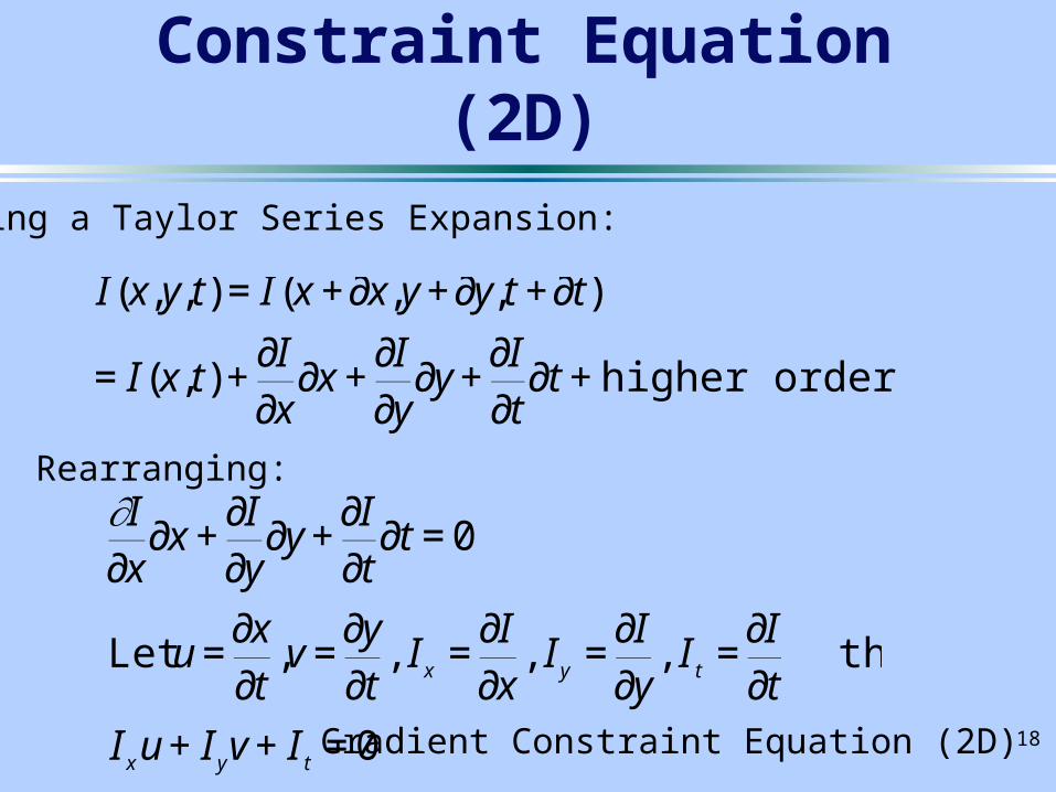
The Gradient Constraint Equation (2D)
Using a Taylor Series Expansion:
€
I(x,y,t) = I(x +∂x,y+∂y,t +∂t)
= I(x,t) +∂I
∂x∂x +
∂I
∂y∂y+
∂I
∂t∂t + higher order terms
Rearranging:
€
∂I∂x∂x +
∂I
∂y∂y+
∂I
∂t∂t = 0
Let u =∂x
∂t,v =
∂y
∂t, Ix =
∂I
∂x, Iy =
∂I
∂y, I t =
∂I
∂t then
Ixu + Iyv+ I t = 0 Gradient Constraint Equation (2D)
19
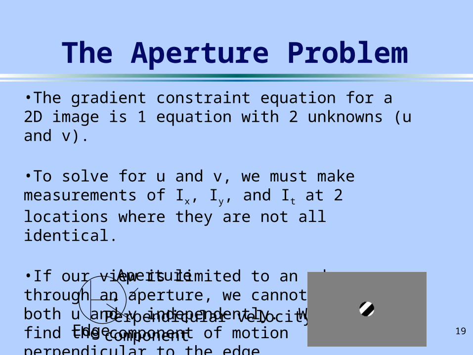
The Aperture Problem•The gradient constraint equation for a 2D image is 1 equation with 2 unknowns (u and v).
•To solve for u and v, we must make measurements of Ix, Iy, and It at 2 locations where they are not all identical.
•If our view is limited to an edge seen through an aperture, we cannot solve for both u and v independently. We can only find the component of motion perpendicular to the edge.
Aperture
EdgePerpendicular velocitycomponent

20
The Aperture Problem is Fundamental
•The aperture problem is a fundamental problem when one is trying to measure image velocity using local detectors.
•This is true in biological vision (neurons have local receptive fields).
•This is also true in machine vision (intensity is detected locally by photodetectors).