a comparative study of simulated and measured main …

American Institute of Aeronautics and Astronautics

1

A Comparative Study of Simulated and Measured

Main Landing Gear Noise for Large Civil Transports

Benedikt König,* Ehab Fares†

Exa GmbH, D-70563 Stuttgart, Germany

Patricio Ravetta‡

AVEC Inc., Blacksburg, Virginia 24060, USA

and

Mehdi R. Khorrami§

NASA Langley Research Center, Hampton, Virginia, 23681, USA

Computational results for the NASA 26%-scale model of a six-wheel main landing gear with and without a

toboggan-shaped noise reduction fairing are presented. The model is a high-fidelity representation of a Boeing

777-200 aircraft main landing gear. A lattice Boltzmann method was used to simulate the unsteady flow around

the model in isolation. The computations were conducted in free-air at a Mach number of 0.17, matching a

recent acoustic test of the same gear model in the Virginia Tech Stability Wind Tunnel in its anechoic configu-

ration. Results obtained on a set of grids with successively finer spatial resolution demonstrate the challenge in

resolving/capturing the flow field for the smaller components of the gear and their associated interactions, and

the resulting effects on the high-frequency segment of the farfield noise spectrum. Farfield noise spectra were

computed based on an FWH integral approach, with simulated pressures on the model solid surfaces or flow-

field data extracted on a set of permeable surfaces enclosing the model as input. Comparison of these spectra

with microphone array measurements obtained in the tunnel indicated that, for the present complex gear

model, the permeable surfaces provide a more accurate representation of farfield noise, suggesting that volu-

metric effects are not negligible. The present study also demonstrates that good agreement between simulated

and measured farfield noise can be achieved if consistent post-processing is applied to both physical and syn-

thetic pressure records at array microphone locations.

I. Introduction

The FAA projects steady growth in air travel during the next two decades.1 The resulting expansion in civil aircraft

operations will require aggressive mitigation of the environmental impact of associated byproducts, such as aircraft

noise, which adversely affect communities surrounding major airports. A prominent component of aircraft noise dur-

ing landing is noise produced by the airframe. Development and advancement of system-level, simulation-based air-

frame noise prediction methodologies, first pursued under the NASA Environmentally Responsible Aviation (ERA)

project, is being vigorously continued as part of the Flight Demonstrations and Capabilities (FDC) project of the

NASA Aeronautics Mission Research Directorate. The undercarriage of an aircraft, in particular the main landing gear

on large civil transports, is the dominant airframe noise source during landing and the most daunting system to simu-

late computationally.

As part of the NASA-Boeing partnership on airframe noise prediction research, a series of building-block model-

and full-scale airframe configurations have been selected to extend the state of the art in simulation-based noise pre-

diction tools to large civil transports. Under this joint effort, the NASA 26%-scale, main landing gear model of a

Boeing 777-200 aircraft serves as the first configuration used to evaluate the capabilities of computational simulations

to accurately predict the aeroacoustic character of an airframe component of extreme geometrical complexity. The

26%-scale main gear model is an ideal configuration, as it corresponds to the most intricate landing gear flown today.

* Principal application engineer, Aerospace, member AIAA. † Senior Technical director, Aerospace, senior member AIAA. ‡ Chief research engineer, senior Member AIAA. § Aerospace engineer, Computational AeroSciences Branch, associate fellow AIAA.


2

The model has been tested extensively in several facilities both in isolated, component-level configuration2-5 and as

part of the 26%-scale semispan STAR (Subsonic Transport Aeroacoustic Research) model of the 777-200 aircraft

tested in the NASA Ames 40- by 80-ft wind tunnel.6 However, validation of the present simulations necessitated the

reacquisition of isolated gear model acoustic measurements under better test conditions and with a more capable mi-

crophone array system. Acoustic results from the most recent test in the Virginia Tech tunnel, reported previously in

Ref. 7, were extensively used for validation of the simulated farfield noise data presented here.

The computational approach used in the present study is built upon the knowledge and experience gained from

previous high-fidelity aeroacoustic simulations of model- and full-scale complete Gulfstream aircraft that were shown

to accurately predict the observed measured trends.8-10 Following that approach, time-dependent simulations of the

26%-scale main gear model were obtained using the Exa Corporation PowerFLOW® lattice Boltzmann flow solver.

The simulations were performed for baseline and treated configurations, where the latter includes a toboggan-shaped

noise-reduction device installed on the gear model.

II. Description of the Landing Gear Model

The high fidelity, 26%-scale, 777 main landing gear model used in this study was originally tested as part of the

STAR model in the NASA Ames 40- by 80-ft wind tunnel.6 This model was also extensively tested at the Virginia

Tech Stability Wind Tunnel (VTSWT), with the tunnel both in hard-wall configuration and an early version of the

anechoic setup.4,5 The high-fidelity model features all the major gear components: strut, braces, torque link, cable

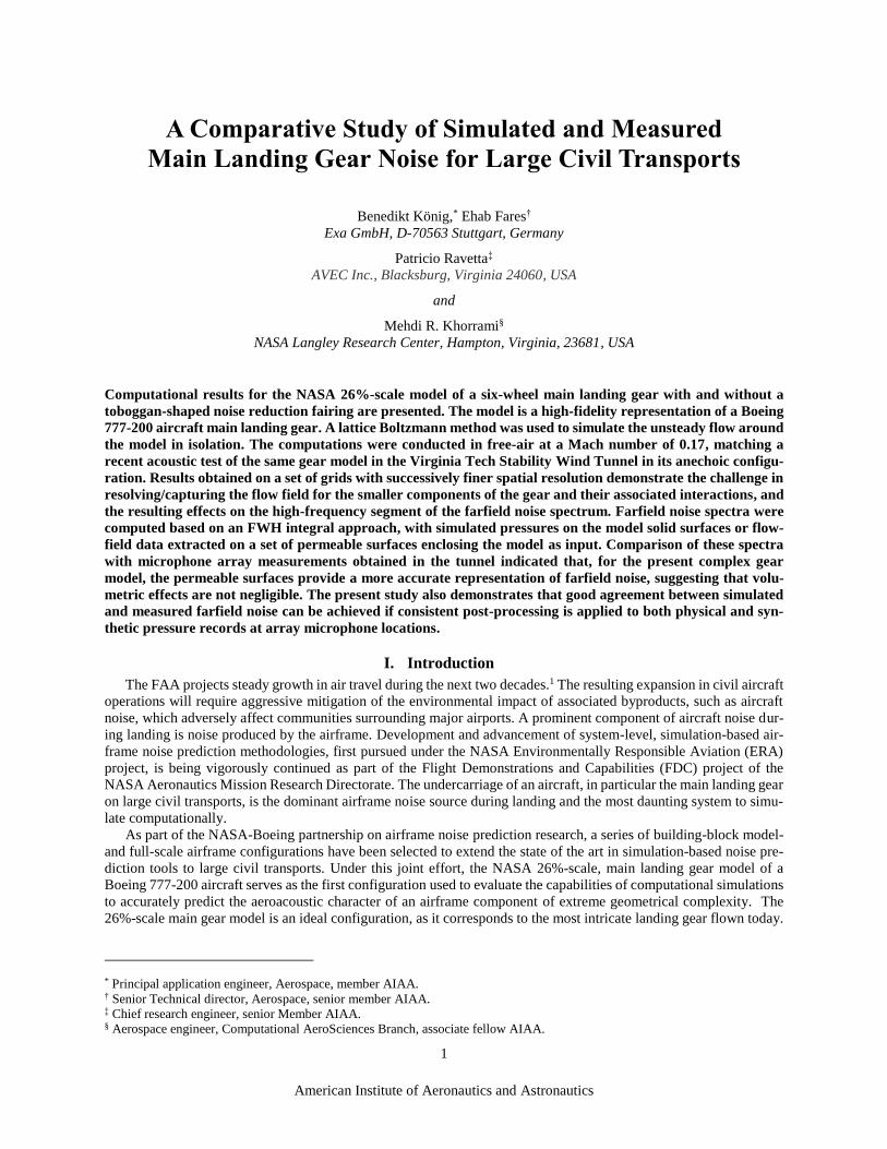
harnesses, lock links, main door, and wheels (see Fig. 1 for the naming convention used throughout this manuscript).

The model also includes most of the details found in the full-scale landing gear, such as oleo lines, cables, wheel hubs,

brake cylinders, and hydraulic valves. The main structure of the model is made of steel and aluminum and the finer

details (gear dressing) were mostly made in stereo lithography up to an accuracy of 3 mm in full-scale. The main

differences with the actual landing gear are: the wheel hubs do not have the openings that allow air to flow freely

through the wheels, a smaller door located near the wing and attached to the main door is not included in the model,

and the wing cavity is not modeled. Results for the baseline configuration with a toe-up truck angle of 13° and those

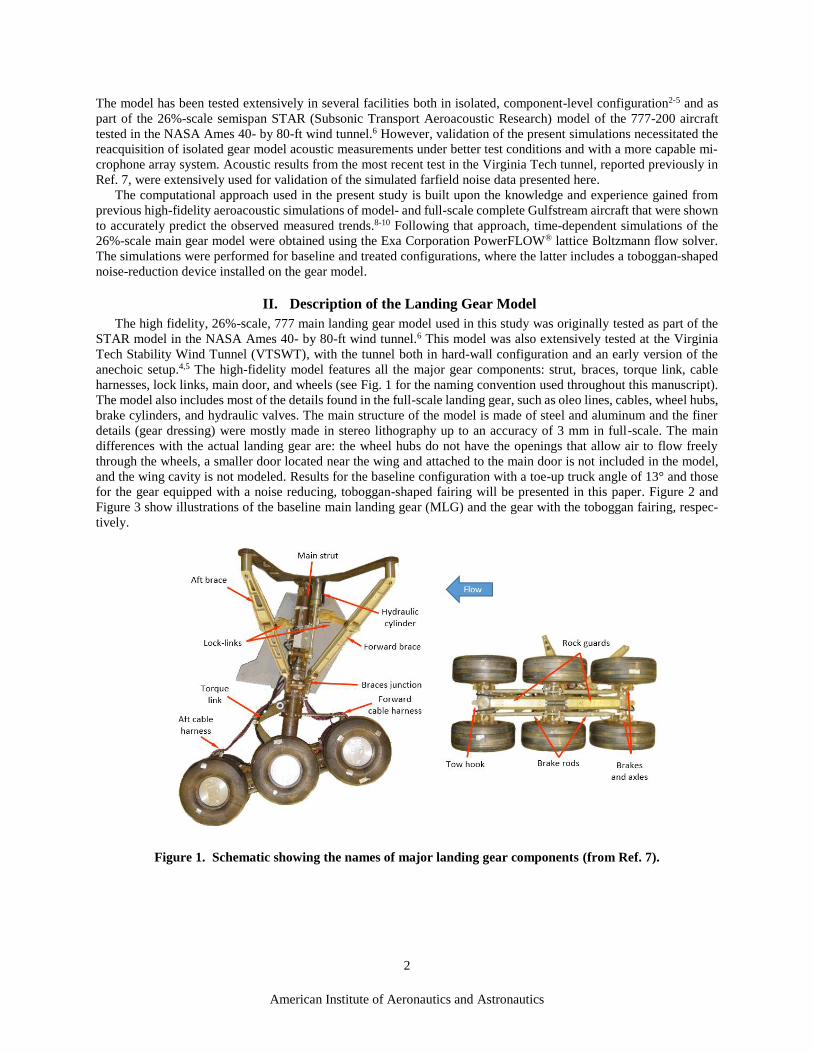
for the gear equipped with a noise reducing, toboggan-shaped fairing will be presented in this paper. Figure 2 and

Figure 3 show illustrations of the baseline main landing gear (MLG) and the gear with the toboggan fairing, respec-

tively.

Figure 1. Schematic showing the names of major landing gear components (from Ref. 7).


3

Figure 2. Illustration of the baseline MLG.

Figure 3. Illustration of the MLG with toboggan

noise reduction concept.

III. Numerical Method

The numerical simulations were performed using PowerFLOW,® which is a flow solver based on the three dimen-

sional 19 state (D3Q19) lattice Boltzmann model (LBM). LBM is a CFD technology developed over the last three

decades11-14 and has been extensively validated for a wide variety of applications ranging from academic direct nu-

merical simulation (DNS) cases to industrial flow problems in the fields of aerodynamics15 and aeroacoustics.8,16,17 In

contrast to methods based on the Navier-Stokes (N-S) equations, LBM uses a simpler and more general physics for-

mulation at the microscopic level.11 The LBM equations recover the macroscopic hydrodynamics of the Navier-Stokes

equations18,19 through the Chapman-Enskog expansion. The local formulation of the LBM equations allows a highly

efficient implementation for distributed computations on thousands of processors. The low dissipation and dispersion

properties of the numerical scheme typically produce aerodynamic and aeroacoustic results that are comparable to

those obtained with classical CFD solvers that use higher-order large eddy simulation (LES), as shown theoretically

in Refs. 19 and 20, and demonstrated in the comparative study of flow over tandem cylinders presented in Ref. 21.

The classical LBM scheme is typically valid in the low Mach number regime up to Mach 0.4. This method was

extended for high subsonic flows up to Mach 0.95 and was mainly applied for the work presented here. Further ex-

tensions to the scheme22,23 that enable solutions at higher transonic and supersonic speeds are also available.

A. Turbulence Modelling

The lattice Boltzmann flow simulation is equivalent to a Direct Numerical Simulation (DNS) of the flow. For high

Reynolds number flows, such as those addressed in this work, the lattice Boltzmann Very Large Eddy Simulation

(LB-VLES) approach described in Refs. 13 and 24 is used to maintain the required computational resources at man-

ageable levels. The approach has been applied previously in Refs. 8, 25, and 26.

B. Wall Treatment

The standard lattice Boltzmann bounce-back boundary condition for no-slip or the specular reflection for free-slip

condition are generalized through a volumetric formulation11,12 near the wall for arbitrarily oriented surface elements

(Surfels) within the Cartesian volume elements (Voxels). This formulation of the boundary condition on a curved

surface cutting the Cartesian grid is automatically mass, momentum, and energy conservative while maintaining the

general spatial second-order accuracy of the underlying LBM numerical scheme. To reduce the resolution require-

ments near the wall for high Reynolds number flows, a hybrid wall function is used to model the region of the boundary

layer closest to the solid surfaces.15,27

C. Complex Geometry Handling and Meshing

The lattice Boltzmann approach is solved on Cartesian meshes. Variable refinement regions (VR) can be defined

to allow for local mesh refinement of the grid size by successive factors of two. Based on the facetized geometry and

the local volume resolution, the model surface is discretized by planar surfels. This process allows the automatic

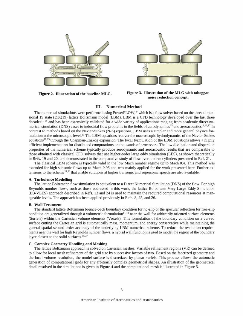
generation of computational grids for any arbitrarily complex geometrical shapes. An illustration of the geometrical

detail resolved in the simulations is given in Figure 4 and the computational mesh is illustrated in Figure 5.


4

Figure 4. Illustration of the overall MLG geometry

including all geometrical details modeled in the sim-

ulations.

Figure 5. Illustration of the mesh around a detail of

the MLG at the fine resolution level.

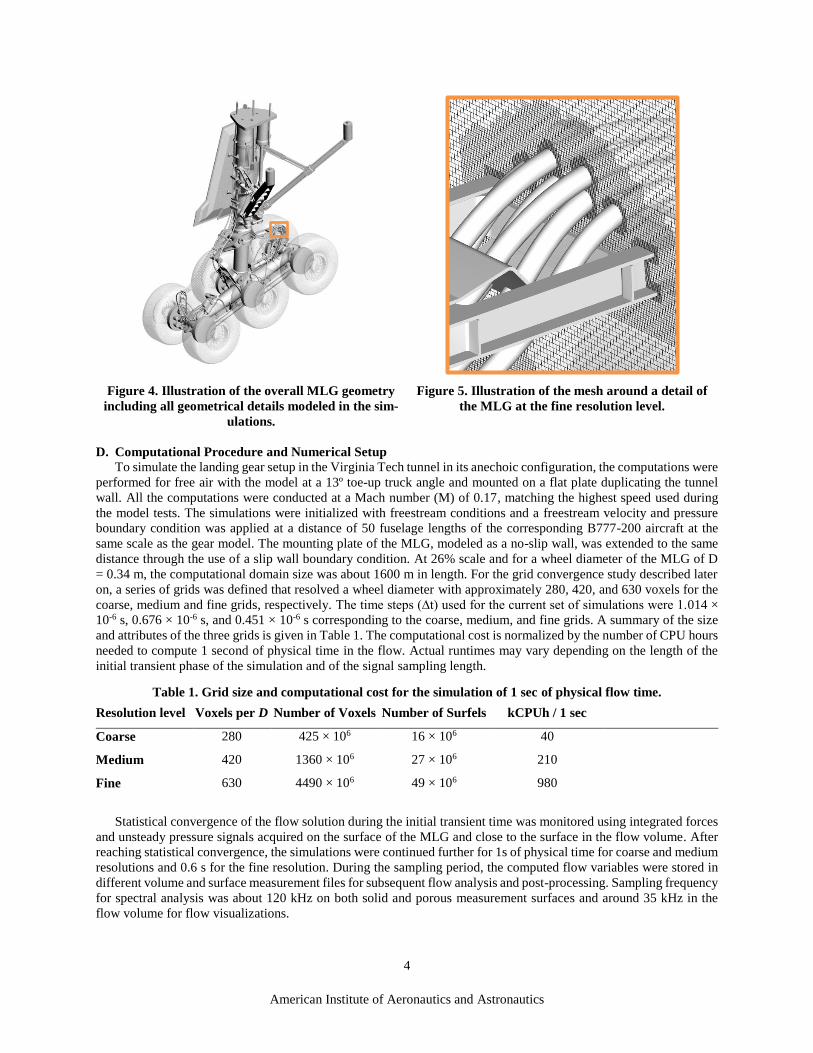
D. Computational Procedure and Numerical Setup

To simulate the landing gear setup in the Virginia Tech tunnel in its anechoic configuration, the computations were

performed for free air with the model at a 13º toe-up truck angle and mounted on a flat plate duplicating the tunnel

wall. All the computations were conducted at a Mach number (M) of 0.17, matching the highest speed used during

the model tests. The simulations were initialized with freestream conditions and a freestream velocity and pressure

boundary condition was applied at a distance of 50 fuselage lengths of the corresponding B777-200 aircraft at the

same scale as the gear model. The mounting plate of the MLG, modeled as a no-slip wall, was extended to the same

distance through the use of a slip wall boundary condition. At 26% scale and for a wheel diameter of the MLG of D

= 0.34 m, the computational domain size was about 1600 m in length. For the grid convergence study described later

on, a series of grids was defined that resolved a wheel diameter with approximately 280, 420, and 630 voxels for the

coarse, medium and fine grids, respectively. The time steps (∆t) used for the current set of simulations were 1.014 ×

10-6 s, 0.676 × 10-6 s, and 0.451 × 10-6 s corresponding to the coarse, medium, and fine grids. A summary of the size

and attributes of the three grids is given in Table 1. The computational cost is normalized by the number of CPU hours

needed to compute 1 second of physical time in the flow. Actual runtimes may vary depending on the length of the

initial transient phase of the simulation and of the signal sampling length.

Table 1. Grid size and computational cost for the simulation of 1 sec of physical flow time.

Resolution level Voxels per D Number of Voxels Number of Surfels kCPUh / 1 sec

Coarse 280 425 × 106 16 × 106 40

Medium 420 1360 × 106 27 × 106 210

Fine 630 4490 × 106 49 × 106 980

Statistical convergence of the flow solution during the initial transient time was monitored using integrated forces

and unsteady pressure signals acquired on the surface of the MLG and close to the surface in the flow volume. After

reaching statistical convergence, the simulations were continued further for 1s of physical time for coarse and medium

resolutions and 0.6 s for the fine resolution. During the sampling period, the computed flow variables were stored in

different volume and surface measurement files for subsequent flow analysis and post-processing. Sampling frequency

for spectral analysis was about 120 kHz on both solid and porous measurement surfaces and around 35 kHz in the

flow volume for flow visualizations.


5

An acoustic analogy approach based on the Ffowcs Williams and Hawkings (FWH) formulation28 was used to

propagate the computed near-field fluctuations to the far field. The employed FWH formulation was based on the

retarded-time formulation 1A by Farassat,29 extended to account for uniform mean flow convection effects to simulate

the noise generated and measured in an ideal infinite wind tunnel30. Integration was performed on a solid surface of

the complete MLG including the mounting-plate and on a permeable surface surrounding the MLG and the mounting-

plate. For the permeable FWH surface, three different options for the outflow region were investigated: open surface,

one single cap, and averaging over a number of end caps31. The permeable surface FWH results presented in this work

are based on averaged end caps.

IV. Experimental Setup and Data Analysis Technique

A. Wind Tunnel Facility

The VTSWT is a continuous, closed circuit, single return, subsonic wind tunnel with a 7.3 m (24 ft) long test

section of dimensions 1.83 by 1.83 m (6 by 6 ft). The tunnel is powered by a 600 hp DC motor driving a 4.26 m (14

ft) propeller that generates a maximum speed of about 280 km/h (255 ft/s) for the empty wind tunnel, i.e., Mach

number (M) of 0.23. The tunnel, which can be operated either in hard wall or anechoic configuration, provides uniform

flow throughout the test section and low turbulence intensity. The data used in the present study were obtained with

the tunnel in its anechoic configuration.5

The upper and lower walls of the 7.3 m long test section are acoustically treated. Large rectangular openings in

the side walls, which extend 5.14 m in the streamwise direction and cover the full 1.83 m height of the test section,

serve as acoustic windows; the remaining surface area of the side walls is acoustically treated. Sound generated inside

the tunnel circuit exits the test section through these acoustic windows into the anechoic chambers on either side.

Large tensioned panels of Kevlar® cloth cover these openings, permitting the sound to pass while containing the bulk

of the flow. The test section arrangement thus simulates a half-open jet, acoustically speaking. The Kevlar® windows

eliminate the need for a jet catcher and, by containing the flow, substantially reduce the lift interference when airfoil

models are tested. Details of the microphone array setup and the acoustic test that generated the data used for compar-

ison in this study are provided in Ref. 7.

B. Data Processing

The FWH propagation approach was used to obtain the time histories of the pressure at the same relative micro-

phone locations used during the wind tunnel test. However, the difference in microphone location due to refraction

effects at the shear layer/Kevlar® wall were ignored in the simulations. To minimize any potential discrepancies related

to the processing algorithms used by AVEC and EXA, both experimental and simulated time histories were beam-

formed using AVEC’s Phased Array software. Although the experimental and simulated data had different sampling

frequencies, the spectral resolution for both data sets was matched to allow a direct comparison of the acoustic maps

and their corresponding integrated results.

Since the shear layer and Kevlar® wall introduce transmission losses, the experimental data had to be corrected to

account for these effects. The corrections used are based on experimental results performed in the empty wind tunnel

described in the literature.32

The beamforming process was performed over a 3D grid surrounding the landing gear with a resolution of 1 cm

in the plane parallel to the array, and 5 cm in the direction normal to it. Diagonal removal beamforming was used to

reduce the impact of uncorrelated noise. The array-integrated spectra were computed for the entire 3D grid surround-

ing the landing gear following the procedure in Ref. 33 (i.e., normalization by the point spread function for a source

at the center of the 3D grid, accounting for diagonal removal, and application of a cutoff level to reduce the contribu-

tion from side lobes).

V. Results and Discussion

A. Effect of Data Surface on FWH Formulation

Initial simulation results of the baseline MLG configuration were used to compare FWH spectra based on solid

and permeable surface formulations. While the spectra showed good agreement in the low frequency range, there were

increasing differences toward higher frequencies. A dedicated investigation was performed to clarify these differences.

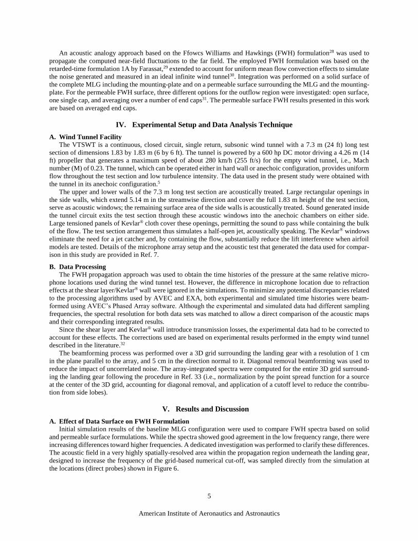
The acoustic field in a very highly spatially-resolved area within the propagation region underneath the landing gear,

designed to increase the frequency of the grid-based numerical cut-off, was sampled directly from the simulation at

the locations (direct probes) shown in Figure 6.


6

Figure 6. Dedicated high-resolution area with direct probes (Grid coarsened for illustration purposes).

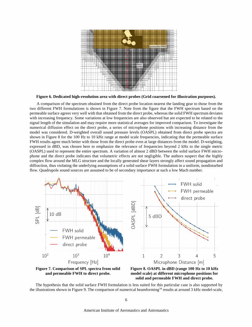
A comparison of the spectrum obtained from the direct probe location nearest the landing gear to those from the

two different FWH formulations is shown in Figure 7. Note from the figure that the FWH spectrum based on the

permeable surface agrees very well with that obtained from the direct probe, whereas the solid FWH spectrum deviates

with increasing frequency. Some variations at low frequencies are also observed but are expected to be related to the

signal length of the simulation and may require more statistical averages for improved comparison. To investigate the

numerical diffusion effect on the direct probe, a series of microphone positions with increasing distance from the

model was considered. D-weighted overall sound pressure levels (OASPL) obtained from direct probe spectra are

shown in Figure 8 for the 100 Hz to 10 kHz range at model scale frequencies, indicating that the permeable surface

FWH results agree much better with those from the direct probe even at large distances from the model. D-weighting,

expressed in dBD, was chosen here to emphasize the relevance of frequencies beyond 2 kHz to the single metric

(OASPL) used to represent the entire spectrum. A variation of almost 2 dBD between the solid surface FWH micro-

phone and the direct probe indicates that volumetric effects are not negligible. The authors suspect that the highly

complex flow around the MLG structure and the locally generated shear layers strongly affect sound propagation and

diffraction, thus violating the underlying assumptions of a solid surface FWH formulation in a uniform, nondisturbed

flow. Quadrupole sound sources are assumed to be of secondary importance at such a low Mach number.

Figure 7. Comparison of SPL spectra from solid

and permeable FWH to direct probe.

Figure 8. OASPL in dBD (range 100 Hz to 10 kHz

model scale) at different microphone positions for

solid and permeable FWH and direct probe.

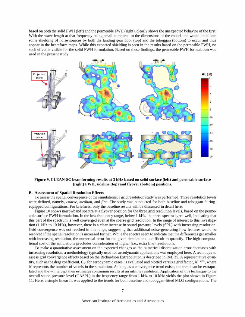
The hypothesis that the solid surface FWH formulation is less suited for this particular case is also supported by

the illustrations shown in Figure 9. The comparison of numerical beamforming34 results at around 3 kHz model-scale,


7

based on both the solid FWH (left) and the permeable FWH (right), clearly shows the unexpected behavior of the first.

With the wave length at that frequency being small compared to the dimensions of the model one would anticipate

some shielding of noise sources by both the landing gear door (top) and the toboggan (bottom) to occur and thus

appear in the beamform maps. While this expected shielding is seen in the results based on the permeable FWH, no

such effect is visible for the solid FWH formulation. Based on these findings, the permeable FWH formulation was

used in the present study.

Figure 9. CLEAN-SC beamforming results at 3 kHz based on solid surface (left) and permeable surface

(right) FWH, sideline (top) and flyover (bottom) positions.

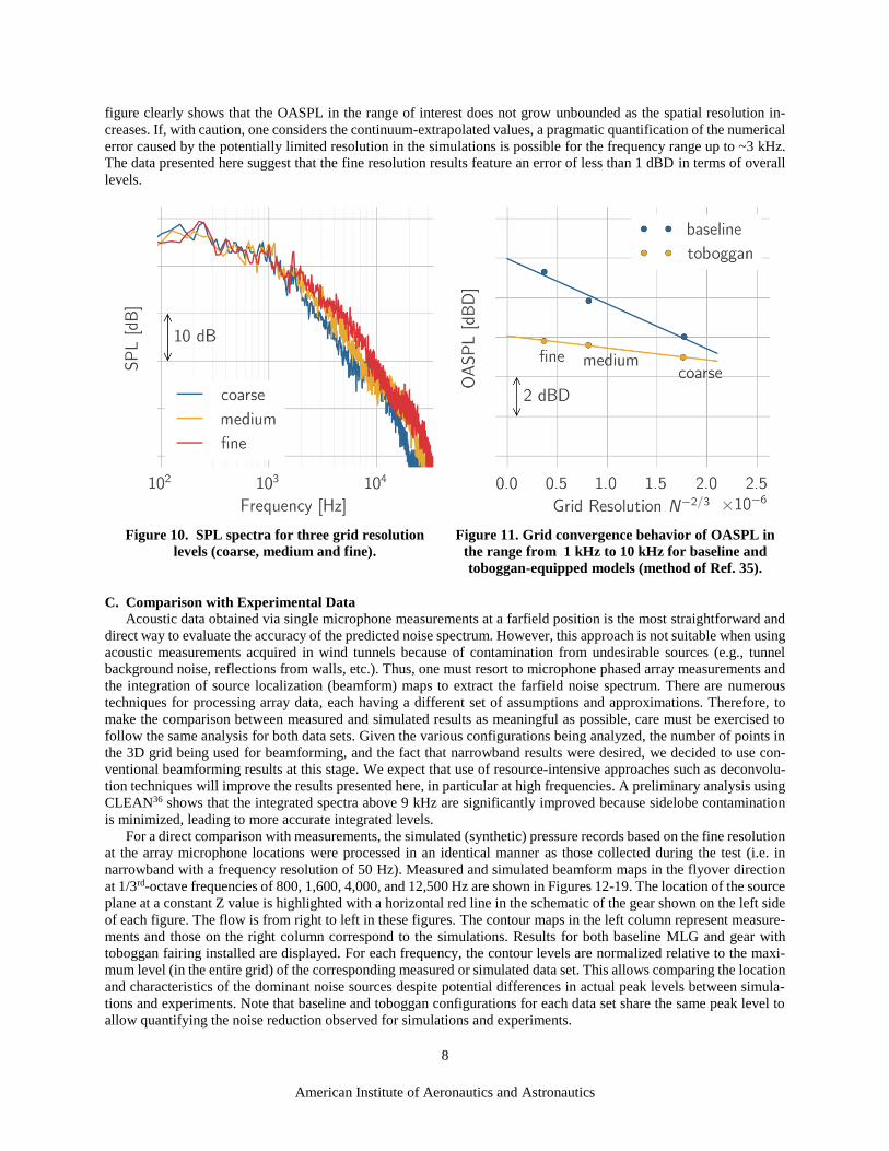
B. Assessment of Spatial Resolution Effects

To assess the spatial convergence of the simulations, a grid resolution study was performed. Three resolution levels

were defined, namely, coarse, medium, and fine. The study was conducted for both baseline and toboggan fairing-

equipped configurations. For briefness, only the baseline results will be discussed in detail here.

Figure 10 shows narrowband spectra at a flyover position for the three grid resolution levels, based on the perme-

able surface FWH formulation. In the low frequency range, below 1 kHz, the three spectra agree well, indicating that

this part of the spectrum is well converged even at the coarse grid resolution. In the range of interest to this investiga-

tion (1 kHz to 10 kHz), however, there is a clear increase in sound pressure levels (SPL) with increasing resolution.

Grid convergence was not reached in this range, suggesting that additional noise-generating flow features would be

resolved if the spatial resolution is increased further. While the spectra seem to indicate that the differences get smaller

with increasing resolution, the numerical error for the given simulations is difficult to quantify. The high computa-

tional cost of the simulations precludes consideration of higher (i.e., extra fine) resolutions.

To make a quantitative assessment on the expected changes as the numerical discretization error decreases with

increasing resolution, a methodology typically used for aerodynamic applications was employed here. A technique to

assess grid convergence effects based on the Richardson Extrapolation is described in Ref. 35. A representative quan-

tity, such as the drag coefficient, CD, for aerodynamic cases, is evaluated and plotted versus a grid factor, 𝑁−2/3, where

N represents the number of voxels in the simulation. As long as a convergence trend exists, the trend can be extrapo-

lated and the y-intercept then estimates continuum results at an infinite resolution. Application of this technique to the

overall sound pressure level (OASPL) in the frequency range from 1 kHz to 10 kHz yields the plot shown in Figure

11. Here, a simple linear fit was applied to the trends for both baseline and toboggan-fitted MLG configurations. The


8

figure clearly shows that the OASPL in the range of interest does not grow unbounded as the spatial resolution in-

creases. If, with caution, one considers the continuum-extrapolated values, a pragmatic quantification of the numerical

error caused by the potentially limited resolution in the simulations is possible for the frequency range up to ~3 kHz.

The data presented here suggest that the fine resolution results feature an error of less than 1 dBD in terms of overall

levels.

Figure 10. SPL spectra for three grid resolution

levels (coarse, medium and fine).

Figure 11. Grid convergence behavior of OASPL in

the range from 1 kHz to 10 kHz for baseline and

toboggan-equipped models (method of Ref. 35).

C. Comparison with Experimental Data

Acoustic data obtained via single microphone measurements at a farfield position is the most straightforward and

direct way to evaluate the accuracy of the predicted noise spectrum. However, this approach is not suitable when using

acoustic measurements acquired in wind tunnels because of contamination from undesirable sources (e.g., tunnel

background noise, reflections from walls, etc.). Thus, one must resort to microphone phased array measurements and

the integration of source localization (beamform) maps to extract the farfield noise spectrum. There are numerous

techniques for processing array data, each having a different set of assumptions and approximations. Therefore, to

make the comparison between measured and simulated results as meaningful as possible, care must be exercised to

follow the same analysis for both data sets. Given the various configurations being analyzed, the number of points in

the 3D grid being used for beamforming, and the fact that narrowband results were desired, we decided to use con-

ventional beamforming results at this stage. We expect that use of resource-intensive approaches such as deconvolu-

tion techniques will improve the results presented here, in particular at high frequencies. A preliminary analysis using

CLEAN36 shows that the integrated spectra above 9 kHz are significantly improved because sidelobe contamination

is minimized, leading to more accurate integrated levels.

For a direct comparison with measurements, the simulated (synthetic) pressure records based on the fine resolution

at the array microphone locations were processed in an identical manner as those collected during the test (i.e. in

narrowband with a frequency resolution of 50 Hz). Measured and simulated beamform maps in the flyover direction

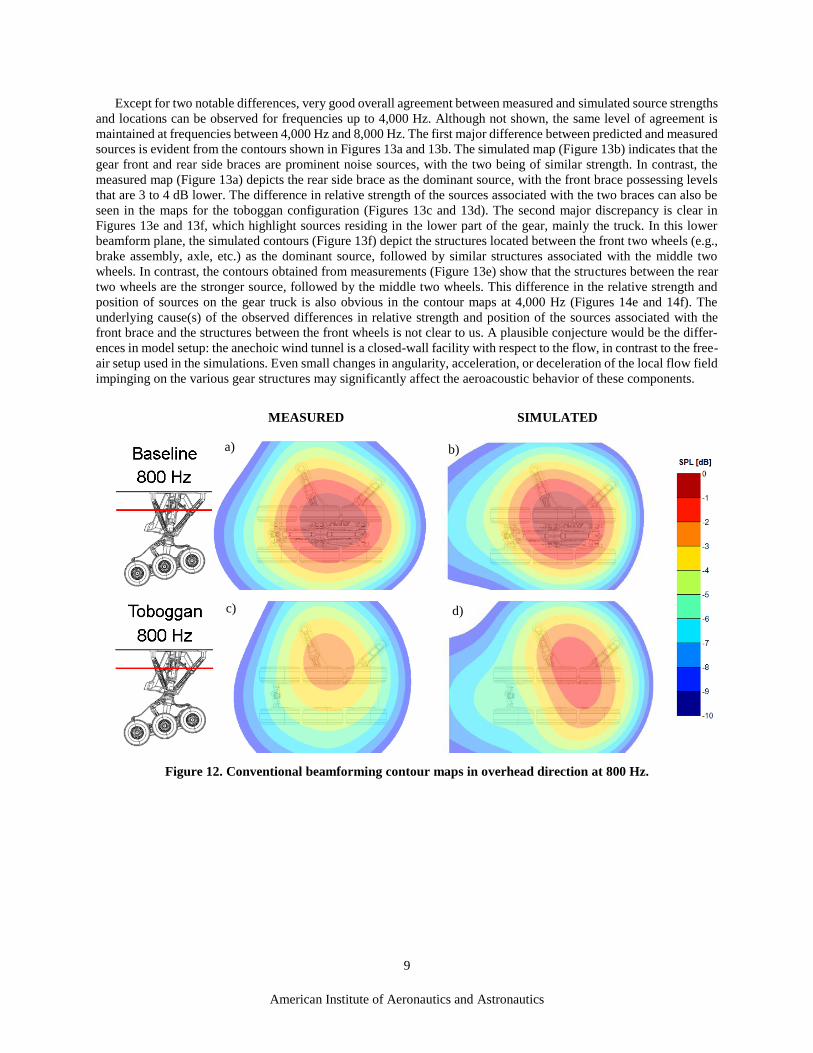
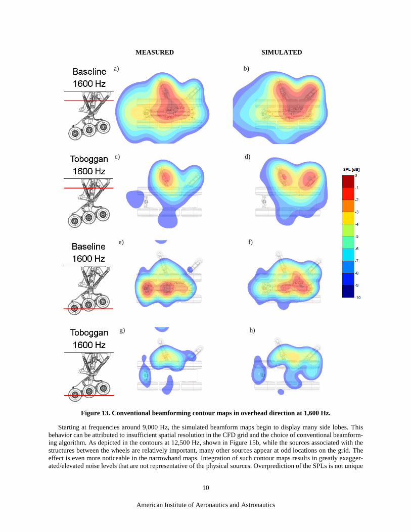
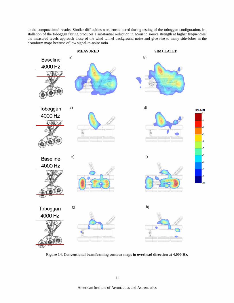
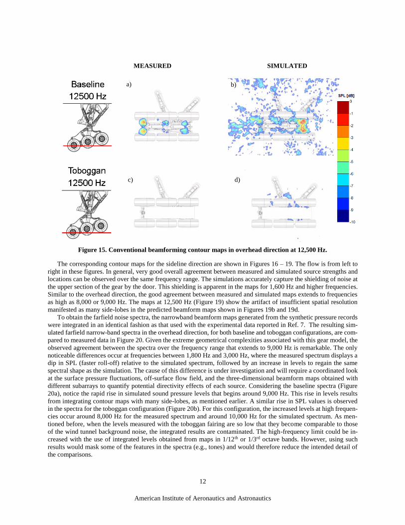
at 1/3rd-octave frequencies of 800, 1,600, 4,000, and 12,500 Hz are shown in Figures 12-19. The location of the source

plane at a constant Z value is highlighted with a horizontal red line in the schematic of the gear shown on the left side

of each figure. The flow is from right to left in these figures. The contour maps in the left column represent measure-

ments and those on the right column correspond to the simulations. Results for both baseline MLG and gear with

toboggan fairing installed are displayed. For each frequency, the contour levels are normalized relative to the maxi-

mum level (in the entire grid) of the corresponding measured or simulated data set. This allows comparing the location

and characteristics of the dominant noise sources despite potential differences in actual peak levels between simula-

tions and experiments. Note that baseline and toboggan configurations for each data set share the same peak level to

allow quantifying the noise reduction observed for simulations and experiments.


9

Except for two notable differences, very good overall agreement between measured and simulated source strengths

and locations can be observed for frequencies up to 4,000 Hz. Although not shown, the same level of agreement is

maintained at frequencies between 4,000 Hz and 8,000 Hz. The first major difference between predicted and measured

sources is evident from the contours shown in Figures 13a and 13b. The simulated map (Figure 13b) indicates that the

gear front and rear side braces are prominent noise sources, with the two being of similar strength. In contrast, the

measured map (Figure 13a) depicts the rear side brace as the dominant source, with the front brace possessing levels

that are 3 to 4 dB lower. The difference in relative strength of the sources associated with the two braces can also be

seen in the maps for the toboggan configuration (Figures 13c and 13d). The second major discrepancy is clear in

Figures 13e and 13f, which highlight sources residing in the lower part of the gear, mainly the truck. In this lower

beamform plane, the simulated contours (Figure 13f) depict the structures located between the front two wheels (e.g.,

brake assembly, axle, etc.) as the dominant source, followed by similar structures associated with the middle two

wheels. In contrast, the contours obtained from measurements (Figure 13e) show that the structures between the rear

two wheels are the stronger source, followed by the middle two wheels. This difference in the relative strength and

position of sources on the gear truck is also obvious in the contour maps at 4,000 Hz (Figures 14e and 14f). The

underlying cause(s) of the observed differences in relative strength and position of the sources associated with the

front brace and the structures between the front wheels is not clear to us. A plausible conjecture would be the differ-

ences in model setup: the anechoic wind tunnel is a closed-wall facility with respect to the flow, in contrast to the free-

air setup used in the simulations. Even small changes in angularity, acceleration, or deceleration of the local flow field

impinging on the various gear structures may significantly affect the aeroacoustic behavior of these components.

MEASURED SIMULATED

Figure 12. Conventional beamforming contour maps in overhead direction at 800 Hz.

a) b)

c) d)


10

MEASURED SIMULATED

Figure 13. Conventional beamforming contour maps in overhead direction at 1,600 Hz.

Starting at frequencies around 9,000 Hz, the simulated beamform maps begin to display many side lobes. This

behavior can be attributed to insufficient spatial resolution in the CFD grid and the choice of conventional beamform-

ing algorithm. As depicted in the contours at 12,500 Hz, shown in Figure 15b, while the sources associated with the

structures between the wheels are relatively important, many other sources appear at odd locations on the grid. The

effect is even more noticeable in the narrowband maps. Integration of such contour maps results in greatly exagger-

ated/elevated noise levels that are not representative of the physical sources. Overprediction of the SPLs is not unique

a) b)

c) d)

e) f)

g) h)


11

to the computational results. Similar difficulties were encountered during testing of the toboggan configuration. In-

stallation of the toboggan fairing produces a substantial reduction in acoustic source strength at higher frequencies:

the measured levels approach those of the wind tunnel background noise and give rise to many side-lobes in the

beamform maps because of low signal-to-noise ratio.

MEASURED SIMULATED


a) b)

c) d)

e) f)

g) h)


12

MEASURED SIMULATED


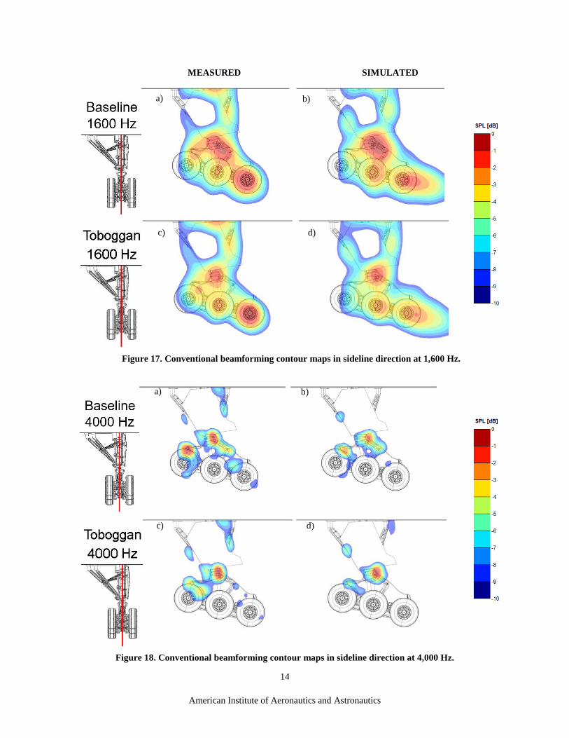
The corresponding contour maps for the sideline direction are shown in Figures 16 – 19. The flow is from left to

right in these figures. In general, very good overall agreement between measured and simulated source strengths and

locations can be observed over the same frequency range. The simulations accurately capture the shielding of noise at

the upper section of the gear by the door. This shielding is apparent in the maps for 1,600 Hz and higher frequencies.

Similar to the overhead direction, the good agreement between measured and simulated maps extends to frequencies

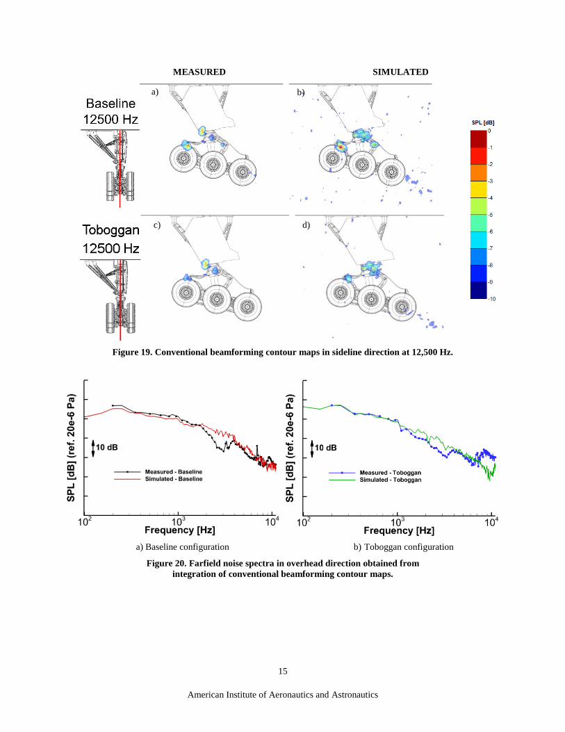
as high as 8,000 or 9,000 Hz. The maps at 12,500 Hz (Figure 19) show the artifact of insufficient spatial resolution

manifested as many side-lobes in the predicted beamform maps shown in Figures 19b and 19d.

To obtain the farfield noise spectra, the narrowband beamform maps generated from the synthetic pressure records

were integrated in an identical fashion as that used with the experimental data reported in Ref. 7. The resulting sim-

ulated farfield narrow-band spectra in the overhead direction, for both baseline and toboggan configurations, are com-

pared to measured data in Figure 20. Given the extreme geometrical complexities associated with this gear model, the

observed agreement between the spectra over the frequency range that extends to 9,000 Hz is remarkable. The only

noticeable differences occur at frequencies between 1,800 Hz and 3,000 Hz, where the measured spectrum displays a

dip in SPL (faster roll-off) relative to the simulated spectrum, followed by an increase in levels to regain the same

spectral shape as the simulation. The cause of this difference is under investigation and will require a coordinated look

at the surface pressure fluctuations, off-surface flow field, and the three-dimensional beamform maps obtained with

different subarrays to quantify potential directivity effects of each source. Considering the baseline spectra (Figure

20a), notice the rapid rise in simulated sound pressure levels that begins around 9,000 Hz. This rise in levels results

from integrating contour maps with many side-lobes, as mentioned earlier. A similar rise in SPL values is observed

in the spectra for the toboggan configuration (Figure 20b). For this configuration, the increased levels at high frequen-

cies occur around 8,000 Hz for the measured spectrum and around 10,000 Hz for the simulated spectrum. As men-

tioned before, when the levels measured with the toboggan fairing are so low that they become comparable to those

of the wind tunnel background noise, the integrated results are contaminated. The high-frequency limit could be in-

creased with the use of integrated levels obtained from maps in 1/12th or 1/3rd octave bands. However, using such

results would mask some of the features in the spectra (e.g., tones) and would therefore reduce the intended detail of

the comparisons.

a) b)

c) d)


13

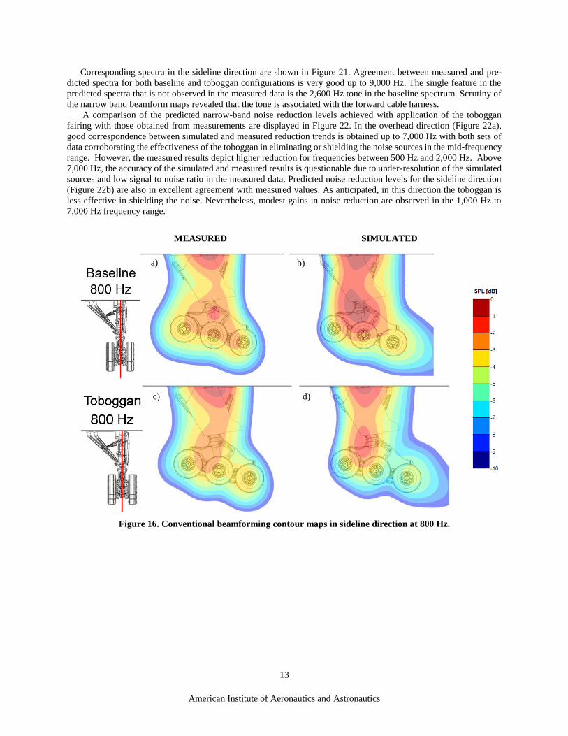
Corresponding spectra in the sideline direction are shown in Figure 21. Agreement between measured and pre-

dicted spectra for both baseline and toboggan configurations is very good up to 9,000 Hz. The single feature in the

predicted spectra that is not observed in the measured data is the 2,600 Hz tone in the baseline spectrum. Scrutiny of

the narrow band beamform maps revealed that the tone is associated with the forward cable harness.

A comparison of the predicted narrow-band noise reduction levels achieved with application of the toboggan

fairing with those obtained from measurements are displayed in Figure 22. In the overhead direction (Figure 22a),

good correspondence between simulated and measured reduction trends is obtained up to 7,000 Hz with both sets of

data corroborating the effectiveness of the toboggan in eliminating or shielding the noise sources in the mid-frequency

range. However, the measured results depict higher reduction for frequencies between 500 Hz and 2,000 Hz. Above

7,000 Hz, the accuracy of the simulated and measured results is questionable due to under-resolution of the simulated

sources and low signal to noise ratio in the measured data. Predicted noise reduction levels for the sideline direction

(Figure 22b) are also in excellent agreement with measured values. As anticipated, in this direction the toboggan is

less effective in shielding the noise. Nevertheless, modest gains in noise reduction are observed in the 1,000 Hz to

7,000 Hz frequency range.

MEASURED SIMULATED

Figure 16. Conventional beamforming contour maps in sideline direction at 800 Hz.

a) b)

c) d)


14

MEASURED SIMULATED

Figure 17. Conventional beamforming contour maps in sideline direction at 1,600 Hz.


a) b)

c) d)

a) b)

c) d)


15

MEASURED SIMULATED


a) Baseline configuration b) Toboggan configuration

Figure 20. Farfield noise spectra in overhead direction obtained from

integration of conventional beamforming contour maps.

a) b)

c) d)


16

a) Baseline configuration b) Toboggan configuration

Figure 21. Farfield noise spectra in sideline direction obtained from

integration of conventional beamforming maps.

a) Overhead direction b) Sideline direction

Figure 22. Reduction in farfield noise levels obtained from integration of conventional beamforming maps.

Noise reduction above ~8 kHz not accurate due to contamination of levels by side-lobes in the maps.

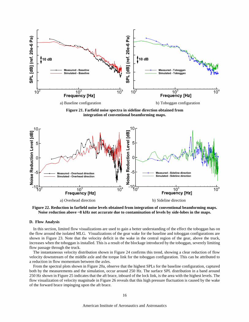
D. Flow Analysis

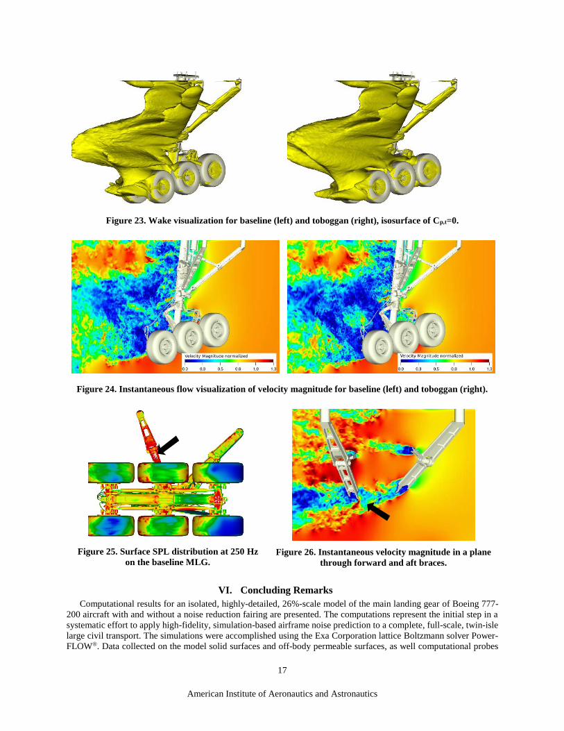
In this section, limited flow visualizations are used to gain a better understanding of the effect the toboggan has on

the flow around the isolated MLG. Visualizations of the gear wake for the baseline and toboggan configurations are

shown in Figure 23. Note that the velocity deficit in the wake in the central region of the gear, above the truck,

increases when the toboggan is installed. This is a result of the blockage introduced by the toboggan, severely limiting

flow passage through the truck.

The instantaneous velocity distribution shown in Figure 24 confirms this trend, showing a clear reduction of flow

velocity downstream of the middle axle and the torque link for the toboggan configuration. This can be attributed to

a reduction in flow momentum between the axles.

From the spectral plots shown in Figure 20a, observe that the highest SPLs for the baseline configuration, captured

both by the measurements and the simulation, occur around 250 Hz. The surface SPL distribution in a band around

250 Hz shown in Figure 25 indicates that the aft brace, inboard of the lock link, is the area with the highest levels. The

flow visualization of velocity magnitude in Figure 26 reveals that this high pressure fluctuation is caused by the wake

of the forward brace impinging upon the aft brace.


17

Figure 23. Wake visualization for baseline (left) and toboggan (right), isosurface of Cp,t=0.

Figure 24. Instantaneous flow visualization of velocity magnitude for baseline (left) and toboggan (right).

Figure 25. Surface SPL distribution at 250 Hz

on the baseline MLG.

Figure 26. Instantaneous velocity magnitude in a plane

through forward and aft braces.

VI. Concluding Remarks

Computational results for an isolated, highly-detailed, 26%-scale model of the main landing gear of Boeing 777-

200 aircraft with and without a noise reduction fairing are presented. The computations represent the initial step in a

systematic effort to apply high-fidelity, simulation-based airframe noise prediction to a complete, full-scale, twin-isle

large civil transport. The simulations were accomplished using the Exa Corporation lattice Boltzmann solver Power-

FLOW®. Data collected on the model solid surfaces and off-body permeable surfaces, as well computational probes


18

imbedded within the flow field, were used to perform an extensive farfield noise study using an FWH integral ap-

proach. The analysis revealed the importance of the volumetric effects on the sound field, rendering solid surface data

as inappropriate for determining the farfield noise signature of a complex gear configuration. To determine solution

convergence behavior, a mesh refinement study was conducted and the effects on the farfield noise spectrum investi-

gated. Despite the highly refined nature of the finest grid used in the current simulations, full convergence of the

computed spectrum at frequencies above 2 kHz remained elusive due to the extreme geometrical complexities and

very fine details inherent in this gear model. A comparative analysis of the simulated results with recent microphone

array measurements of the same gear model obtained in the Virginia Tech wind tunnel in its anechoic configuration

was conducted using AVEC’s Phased Array software. Synthetic pressure records at the same array microphone loca-

tions in the tunnel were used to generate the beamform contour maps for the baseline gear model and the configuration

with the toboggan fairing installed. The simulated maps were in close agreement with those obtained from measured

data, for frequencies up to 9 kHz for both overhead and sideline directions. Comparison of simulated and measured

farfield noise spectra obtained from integration of the beamform maps displays remarkable agreement for frequencies

up to 8 kHz, affirming the capability of such simulations to accurately predict the airframe noise of a large civil

transport.

Acknowledgments

This work was partially supported by the Environmentally Responsible Aviation (ERA) and Flight Demonstrations

and Capabilities (FDC) projects under the Integrated Aviation Systems Program (IASP) of NASA. The authors grate-

fully acknowledge the invaluable contribution of Scott Brynildsen of Craig Technologies, for providing geometry

modifications and CAD support. We would also like to express our sincere appreciation to Patrick Moran of the NASA

Ames Research Center for high-quality visualizations and animations of the large data sets. All the simulations were

performed on the Pleiades supercomputer at the NASA Advanced Supercomputing (NAS) facility at Ames Research

Center. The logistical support provided by NAS staff is greatly appreciated.

References 1https://www.faa.gov/data_research/aviation/aerospace_forecasts/media/FY2016-36_FAA_Aerospace_Forecast.pdf,

last accessed October 24, 2016. 2Jaeger, S. M., Burnside, N. J., Soderman, P. T., Horne, W. C., and James, K. D., “Microphone Array Assessment of

an Isolated, 26%-Scale, High Fidelity Landing Gear,” AIAA Paper 2002-2410, June 2002. 3Ravetta, P. A., Burdisso, R. A., and Ng, W. F., “Wind Tunnel Aeroacoustic Measurements of a 26%-scale 777 Main

Landing Gear Model,” AIAA Paper 2004-2885, May 2004. 4Ravetta, P. A., Burdisso, R. A., Ng, W. F., Khorrami, M. R., and Stoker, R. W., “Screening of Potential Noise Control

Devices at Virginia Tech for QTD II Flight Test,” AIAA Paper 2007-3455, May 2007. 5Remillieux, M. C., Camargo, H. E., Ravetta, P. A., Burdisso, R. A., and Ng, W. F., “Novel Kevlar-Walled Wind

Tunnel for Aeroacoustic Testing of a Landing Gear,” AIAA Journal, Vol. 46, No. 7, July 2008, pp. 1631 – 1639. 6Horne, W. C., James, K. D., Arledge, T. K., Soderman, P. T., Burnside, N., and Jaeger, S. M., “Measurements of

26%-scale 777 Airframe Noise in the NASA Ames 40- by 80 Foot Wind Tunnel,” AIAA Paper 2005-2810, May

2005. 7Ravetta, P. A., Khorrami, M. R., Burdisso, R. A., and Wisda, D. M., “Acoustic Measurements of a Large Civil

Transport Main Landing Gear Model,” AIAA Paper 2016-2901, May-June 2016. 8Khorrami, M. R., Fares, E., and Casalino, D., “Towards Full-Aircraft Airframe Noise Prediction: Lattice-Boltzmann

Simulations,” AIAA Paper 2014-2481, June 2014. 9Khorrami, M. R., and Fares, E., “Simulation-Based Airframe Noise Prediction of a Full-Scale Full Aircraft,” AIAA

Paper 2016-2706, May-June 2016. 10Fares, E., Duda, B., and Khorrami, M. R., “Airframe Noise Prediction of a Detailed Full Aircraft in Model and Full

Scale Using a Lattice Boltzmann Approach,” AIAA Paper 2016-2707, May-June 2016. 11Chen, H., “Volumetric Formulation of the Lattice-Boltzmann Method for Fluid Dynamics: Basic Concept,” Physical

Review E, Vol. 58, No. 3, 1998, pp. 3955 – 3963, doi: dx.doi.org/10.1103/PhysRevE.58.3955. 12Chen, H., Texeira, C., and Molvig, K., “Realization of Fluid Boundary Condition via Discrete Boltzmann

Dynamics,” Int. Journal of Modern Physics C, Vol. 9, No. 8, 1998, pp. 1281 – 1292. 13Chen, H., Kandasamy, S., Orszag, A., Shock, R., Succi, S., and Yakhot, V., “Extended Boltzmann Kinetic Equation

for Turbulent Flows,” Science, No. 301, 2003, pp. 633 – 636.

https://www.faa.gov/data_research/aviation/aerospace_forecasts/media/FY2016-36_FAA_Aerospace_Forecast.pdf


19

14Chen, S. and Doolen, G., “Lattice Boltzmann Method for Fluid Flows,” Annual Review of Fluid Mechanics, Vol.

30, 1998, pp. 329 – 364. 15Fares E. and Nölting, S., “Unsteady Flow Simulation of a High-Lift configuration using Lattice-Boltzmann

Approach,” AIAA Paper 2011-869, January 2011. 16Casalino, D., Nölting, S., Fares, E., Van de Ven, T., Perot, F., and Bres, G., “Towards Numerical Aircraft Noise

Certification: Analysis of a Full-Scale Landing Gear in Fly-Over Configuration,” AIAA Paper 2012-2235, June 2012. 17Casalino, D., Ribeiro, A. F. P., Fares, E., Nölting, S., Mann, A., Perot, F., Li, Y., Lew, P. T., Sun, C., Gopalakrishnan,

P., Zhang, R., Chen, H., and Habibi, K., “Towards Lattice-Boltzmann Prediction of Turbofan Engine Noise,” AIAA

Paper 2014-3101, June 2014. 18Chen, H., Chen S., and Matthaeus, W. H., “Recovery of the Navier-Stokes equations using a lattice-gas Boltzmann

method,” Physical Review A, No. 45, 1992, pp. R5339 – R5342, doi: http://dx.doi.org/10.1103/PhysRevA.45.R5339. 19Qian, Y. H., D'Humières, D., and Lallemand, P., “Lattice BGK Models for Navier-Stokes Equation,” Europhysics

Letters, Vol. 17, 1992, pp. 479 – 484, doi:10.1209/0295-5075/17/6/001. 20Marié, S., Ricot D., and Sagaut, P., “Comparison between lattice Boltzmann method and Navier–Stokes high order

schemes for computational aeroacoustics,” Journal of Computational Physics, Vol. 228, 2009, pp. 1056-1070,

doi:10.1016/j.jcp.2008.10.021. 21Lockard, D. P., “Summary of the Tandem Cylinder Solutions from the Benchmark problems for Airframe Noise

Computations-I Workshop,” AIAA paper 2011-353, January 2011, doi:10.2514/6.2011-353. 22Shan, X., Yuan, X. F., and Chen, H., “Kinetic theory representation of hydrodynamics:a way beyond the Navier–

Stokes equation,” Journal of Fluid Mechanics, Vol. 550, March 2006, pp. 413 – 441. 23Zhang, R., Shan, X., and Chen, H., “Efficient kinetic method for fluid simulation beyond the Navier-Stokes

equation,” Physical Review E, October 2006, p. 046703, doi: 10.1103/PhysRevE.74.046703. 24Yakhot, V., and Orszag, S. A., “Renormalization Group Analysis of Turbulence. I. Basic Theory,” Journal of

Scientific Computing, Vol. 1, No. 1, 1986, pp. 3 – 51. 25Fares, E., Casalino, D., and Khorrami, M. R., “Evaluation of Airframe Noise Reduction Concepts via Simulations

Using a Lattice Boltzmann Approach,” AIAA Paper 2015-2988, June 2015. 26Khorrami, M. R., Mineck, R., Yao, C., and Jenkins, N., “A Comparative Study of Simulated and Measured Gear-

Flap Flow Interaction,” AIAA Paper 2015-2989, May 2015. 27Fares, E., “Unsteady Flow Simulation of the Ahmed Reference Body using a Lattice Boltzmann Approach,” Journal

of Computers and Fluids, No. 35, 2006, pp. 940 – 950, doi:10.1016/j.compfluid.2005.04.011. 28Hawking, J. E., and Ffowcs Williams, D. L., “Sound Generation by Turbulence and Surfaces in Arbitrary Motion,”

Philosophical Transactions of the Royal Society of London, Series A, Mathematical and Physical Sciences, Vol. 264,

No. 1151, 1969, pp. 321 – 342. 29Farassat, F., and Succi, G., “The Prediction of Helicopter Discrete Frequency Noise,” Vertica, Vol. 7, No. 4, 1983,

pp. 309 – 320. 30Najafi-Yazdi, A., Brès, G. A., and Mongeau, L., “An Acoustic Analogy Formulation for Moving Sources in

Uniformly Moving Media,” Proceeding of The Royal Society of London A, Vol. 467, No. 2125, 2011, pp. 144 – 165. 31Shur, M., Spalart P., and Strelets, M. K., “Noise Prediction for Increasingly Complex Jets. Part I, Methods and Tests;

Part II Applications,” International Journal of Aeroacoustics, Vol. 4, No. 3, 2005, pp. 213 – 245. 32Devenport, W. J., Burdisso, R. A., Borgoltz, A., Ravetta P. A., Barone, M. F., Brown, K. A., and Morton, M. A.,

“The Kevlar-walled anechoic wind tunnel,” Journal of Sound and Vibration, Vol. 332, No. 17, August 2013, pp.

3971–3991. 33Mueller, T. (ed.), Aeroacoustic Measurements, Springer, 2002. ISBN 3-540-41757-5. 34Lockard, D. P., Humphreys, W. M., Khorrami, M. R., Fares, E., Casalino, D., and Ravetta, P. A., “Comparison of

Computational and Experimental Microphone Array Results for an 18%-Scale Aircraft Model,” AIAA Paper 2015-

2990, May 2015. 35Levy, D. W., Laflin, K. R., Tinoco, E. N., Vassberg, J. C., Mani, M., Rider, B., Rumsey, C. L., Wahls, R. A.,

Morrison, J. H., Brodersen, O. P., Crippa, S., Mavriplis, D. J., and Murayama, M., “Summary of Data from the Fifth

AIAA CFD Drag Prediction Workshop,” AIAA Paper 2013-0046, January 2013. 36Sijtsma, T., “CLEAN Based on Spatial Source Coherence,” AIAA Paper 2007-3436, May 2007.

a comparative study of simulated and measured main …

Documents