Send Orders for Reprints to reprints@benthamscience.ae

The Open Electrical & Electronic Engineering Journal, 2017, 11, 23-37 23

1874-1290/17 2017 Bentham Open

The Open Electrical & ElectronicEngineering Journal

Content list available at: www.benthamopen.com/TOEEJ/

DOI: 10.2174/1874129001711010023

RESEARCH ARTICLE

A Chaotic Quantum Behaved Particle Swarm Optimization Algorithmfor Short-term Hydrothermal Scheduling

Chen Gonggui*, 1, Huang Shanwai1 and Sun Zhi2

1Key Laboratory of Industrial Internet of Things & Networked Control, Ministry of Education, Chongqing University ofPosts and Telecommunications, Chongqing 400065, China2Guodian Enshi Hydropower Development, Enshi, 445000, China

Received: May 05, 2016 Revised: November 03, 2016 Accepted: November 29, 2016

Abstract: This study proposes a novel chaotic quantum-behaved particle swarm optimization (CQPSO) algorithm for solving short-term hydrothermal scheduling problem with a set of equality and inequality constraints. In the proposed method, chaotic local searchtechnique is employed to enhance the local search capability and convergence rate of the algorithm. In addition, a novel constrainthandling strategy is presented to deal with the complicated equality constrains and then ensures the feasibility and effectiveness ofsolution. A system including four hydro plants coupled hydraulically and three thermal plants has been tested by the proposedalgorithm. The results are compared with particle swarm optimization (PSO), quantum-behaved particle swarm optimization (QPSO)and other population-based artificial intelligence algorithms considered. Comparison results reveal that the proposed method cancope with short-term hydrothermal scheduling problem and outperforms other evolutionary methods in the literature.

Keywords: Short-term hydrothermal scheduling, Quantum-behaved particle swarm optimization, Chaotic local search, Constrainshandling.

1. INTRODUCTION

The short-term hydrothermal scheduling (SHTS) as a significant and constrained optimization problem plays a vitalrole in power system. The complex and nonlinear peculiarities of SHTS problem make finding the efficient globaloptimal solution a huge challenge. The objective of SHTS is the determination of power generations among hydroplants and thermal plants with the result that the fuel cost of thermal plants is minimized over a schedule horizon of oneday when meeting various hydraulic and electrical operational constraints. Usually, the constraints include system loadbalance, initial and terminal reservoir storage volume limits as well as water dynamic balance as the equality constraintsand power limits of thermal plants and hydro plants, reservoir storage volume limits as well as discharge limits of hydroplants as the inequality constraints.

In the past few decades, many methods are implemented for solving the SHTS problem such as dynamicprogramming (DP) [1], linear programming (LP) [2] and Lagrange relaxation (LR) [3]. DP algorithm can actuallytackle a quite general class of dynamic optimization problems, including the ones with nonlinear constraints. It has beenwidely used to solve short-term hydrothermal scheduling problem. However, the disadvantage of DP is obvious withthe growth of computational and dimensional requirements in a larger system. The linear programming method is aimedat linearizing the hydro power generation depending on water discharge so as to ignore the head change effect andreduce the accuracy of the solution. The basic idea of Lagrange relaxation method is to relax demand and reserverequirements using Lagrange multipliers.

* Address correspondence to this author at the Key Laboratory of Industrial Internet of Things & Networked Control, Ministry of Education,Chongqing University of Posts and Telecommunications, Chongqing 400065, China; Tel: + 86-15616106539; Fax: +86-23-62461585; E-mail:chenggpower@126.com.

24 The Open Electrical & Electronic Engineering Journal, 2017, Volume 11 Gonggui et al.

LR method is efficient in dealing with large-scale problems, however, it is easy to generate dual optimal solution whichrarely satisfies the power balance and reserve constraints. Additionally, the convergence and accuracy of LR depend onthe Lagrange multipliers updating methods. In general, those traditional methods have lost the superiority when facedwith the complicated nonlinear constraints and the non-convex short-term hydrothermal scheduling problem.

Other than the above methods, many artificial intelligence algorithms have been successfully applied to overcomethe drawbacks of traditional algorithms in many areas including short-term hydrothermal scheduling problem [4, 5].Typical algorithms such as evolutionary programming (EP) [6], genetic algorithm (GA) [7], differential evolution (DE)[8, 9] clonal selection (CS) [10] and particle swarm optimization (PSO) [11] have obtained good effect. However, thosealgorithms are easy to trap into the local optimum and sensitive to initial point which may debase the solution quality aswell as effectiveness. The main disadvantage of PSO algorithm maybe is that, it does not guarantee to be globalconvergent, and sensitive to initial point although it converges fast. Compared with PSO, quantum-behaved PSO haslesser parameters to control and better search capability. However, the conventional QPSO algorithm still suffers slowconvergence for complex and large-scale SHTS problems. Hence, in this paper, a chaotic local search technique isemployed to enhance local search capability in exploring the global best solution. The chaotic optimization methodtakes advantage of the universality, randomicity, sensitivity dependence on initial conditions and it is more likely toacquire the global optimum solution. Thus, the proposed chaotic quantum behaved particle swarm optimization(CQPSO) algorithm is implemented to solve short-term hydrothermal scheduling problem in a four hydro plants andthree thermal plants system. The simulation results show that the proposed method is able to obtain higher qualitysolutions.

This paper is organized as follows. Section 2 describes the mathematical formulation of SHTS problem. Section 3introduces the PSO and QPSO briefly. Section 4 proposes a chaotic quantum behaved particle swarm optimizationalgorithm for solving SHTS problem. Section 5 presents the simulation experiments and results. Finally, theconclusions are provided in section 6.

2. PROBLEM FORMULATION

The objective of the SHTS problem is to minimize the total cost of thermal plant as much as possible while makingfull use of hydro resource. Generally, the scheduling period and the scheduling time interval are set to 24h and 1hrespectively. The objective function and related equality and inequality constraints can be simulated as follows.

2.1. Objective Function

The objective function of the problem is formulated as follows:

(1)

Taking the valve-point effects into consideration, the fuel cost function can be expressed as the sum of a quadraticfunction and a sinusoidal function as follows:

(2)

where F is the total fuel cost; fi(Psi,t) is fuel cost of the ith thermal plant at time interval t; Psi,t is the generation of theith thermal plant at time interval t; asi, bsi and csi are cost coefficients of the ith thermal plants; dsi, esi are value-pointeffects coefficients of the ith thermal plants; Ns is the number of thermal plants; T is the number of intervals over ascheduling horizon.

,

1 1

2 min

, , ,

1 1

min ( )

sin( ( ))

s

s

NT

i si t

t i

NT

si si si t si si t si si si si t

t i

F f P

a b P c P d e P P

2

, ,

1 1

min sNT

si si si t si si t

t i

F a b P c P

A Chaotic Quantum Behaved Particle The Open Electrical & Electronic Engineering Journal, 2017, Volume 11 25

2.2. Constraints

2.2.1. System Load Balance

(3)

where Nh is the number of hydro plants; Phj,t is the generation of the jth hydro plant at time interval t; PD,t is the loaddemand at time interval t; PL,t is the power loss at time interval t, which can be calculated by Kron’s formula [6]:

(4)

where B, B, B00 are power loss coefficients. The power generation of hydro plants is represented as a function ofreservoir storage volume and water discharge as:

(5)

where Vj,t is reservoir storage volume of the jth hydro plant at time interval t; Qj,t is water discharge of the jth hydroplant at time interval t; C1j, C2j, C3j, C4j, C5j and C6j represent hydro power generation coefficients.

2.2.2. Output Power Constraints

(6)

where Psi,min and Psi,max are the minimum and maximum power generation of the ith thermal plant; Phj,min and Phj,max arethe minimum and maximum power generation of the jth hydro plant;

2.2.3. Thermal Unit Ramp Rate Limits

(7)

where URi and DRi are ramp-up and ramp-down rate limits of the ith thermal unit respectively.

2.2.4. Reservoir Storage Volume Limits

(8)

where Vj,min and Vj,max are the minimum and maximum reservoir storage volume limits of the jth hydro plant.

2.2.5. Water Discharge Limits

(9)

where Qj,min and Qj,max are the minimum and maximum water discharge limits of the jth hydro plant.

2.2.6. Initial and Terminal Reservoir Storage Volumes Limits

(10)

, , , ,

1 1

; 1,2,...,s hN N

si t hj t D t L t

i j

P P P P t T

, , , 0 , 00

1 1 1

s h sN N N

L t si t ij si t i si t

i j i

P P B P B P B

2 2

, 1 , 2 , 3 , , 4 ,

5 , 6

( ) ( )

; 1,2,..., , 1,2,...,

hj t j j t j j t j j t j t j j t

j j t j h

P C V C Q C V Q C V

C Q C j N t T

,min , ,max

,min , ,max

si si t si

hj hj t hj

P P P

P P P

, , 1

, 1 ,

1,2,..., , 1,2,...,si t si t i

s

si t si t i

P P URi N t T

P P DR

,min , ,max ; 1,2,...,j j t jV V V t T

,min , ,max ; 1,2,...,j j t jQ Q Q t T

,0 ,B , ,E, ; 1,2,...,j j j T j hV V V V j N= = =

26 The Open Electrical & Electronic Engineering Journal, 2017, Volume 11 Gonggui et al.

where Vj,B and Vj,E are the initial and terminal reservoir storage volumes limits of the jth hydro plant.

2.2.7. Water Dynamic Balance

(11)

where Ij,t, Sj,t are the nature inflow and water spillage of the jth hydro plant at time interval t; Nj is number ofupstream plants directly connected with hydro plant j; τhj is the time delay from the upstream hydro plant h to plant j.

3. OVERVIEW OF QUANTUM BEHAVED PARTICLE SWARM OPTIMIZATION

3.1. Particle Swarm Optimization

Particle swarm optimization (PSO) algorithm was put forward by Eberhart and Kennedy in 1995. It is a populationbased stochastic algorithm to find an optimum solution of a problem [12]. The algorithm is different from evolutionaryalgorithms; however it is much simpler since it has no use for selection. In PSO, each candidate solution named as“particle” flies around the solution space and lands on the optimal position. All the particles are evolved by competitionand cooperation according to fitness functions. Each particle has a memory and keeps track of its own personal bestsolution (Pbest) and the global best solution (Gbest).

Assume that there are N particles in a D-dimensional space, the position and velocity vectors particle can berepresented as xi = (xi1, xi2… xiD) and vi = (vi1, vi2… viD) where i = 1, 2… N. The updating formulas of position andvelocity of the ith particle can be described as follows:

(12)

(13)

where w is velocity inertia weight; r1 and r2 are two random numbers from the interval [0, 1]; c1 and c2 are thecognitive and social parameters; k is the current iteration; Pbest stands for the best solution of the all swarm founded attime k and Gbest represents the best solution until time k.

3.2. Quantum Behaved Particle Swarm Optimization

Though PSO algorithm is characterized by fast convergence, but it has no guarantee to be global convergence. Inorder to solve this problem, QPSO, as a variant of PSO, was proposed by Sun et al. [13] in 2004, when they wereinspired by quantum mechanics and fundamental theory of particle swarm. In QPSO, quantum theory is applied in thesearching process. Because of the uncertainty principle of quantum mechanics, the position and velocity of a particlecannot be determined synchronously in quantum world. New state of each particle is determined by wave functionψ(x,t) [14]. In literature [15], Clerc and Kennedy analyze the trajectory of each particle in PSO and assume that eachparticle can converge to its local attractor which can guarantee the global convergence. The local attractor is defined asfollows:

(14)

where ϕ = c1r1/ (c1r1 + c2r2); r1 and r2 are values generated according to a uniform in range [0, 1]; c1 and c2 are thecognitive and social parameters. According to the Monte Carlo method, the particles update their positions by thefollowing iterative equation:

(15)

, , 1 , , , , ,

1

( )

1,2,..., , 1,2,...,

s

hj hj

N

j t j t j t j t j t h t h t

i

h

V V I Q S Q S

j N t T

1

1 1 2 2( ) ( )k k k k k k k

i i best i best iv w v c r G x c r P x+ = + - + -

1 1k k k

i i ix x v+ += +

, , ,( (1.0 ) ); 1,2,..., , 1,2,...,k k k

i j i j g jp P P i N j D = + - = =

1

, , , ,

1

, , , ,

In(1/ ), if 0.5

In(1/ ), if 0.5

k k k k

i j i j best j i j

k k k k

i j i j best j i j

x p M x u rd

x p M x u rd

A Chaotic Quantum Behaved Particle The Open Electrical & Electronic Engineering Journal, 2017, Volume 11 27

where β is a design parameter called contraction-expansion coefficient; u and rd are probability distribution randomnumbers in the interval [0, 1]. Mbest is the mean of the Pbest position of all particles and it can be formulated as:

(16)

The steps of QPSO are depicted as follows from Coelho [16, 17].

Step 1: Initialize randomly the initial particles in the feasible range using a uniform probability distributionfunction.Step 2: Evaluate the fitness value of each particle.Step 3: Compare the fitness of each particle with Pbest value. If current fitness value is better than Pbest then setcurrent fitness value to Pbest.Step 4: Compare Pbest values with current Gbest value. If Pbest values are better than Gbest, replace Gbest with currentPbest.Step 5: Calculate the Mbest using Eq.(16).Step 6: Update the position of the particles according to Eq.(15).Step 7: Repeat Step 2 to Step 7 until termination criteria is met.

4. CHAOTIC QUANTUM BEHAVED PARTICLE SWARM OPTIMIZATION FOR SOLVING SHTS

Chaos is a deterministic, random-like mathematical phenomenon which takes place in nonlinear systems andstrongly affected by the initial conditions [18]. This kind of unpredictability of random behavior is also helpful indealing with SHTS problem. Thus, chaos was widely utilized in order to generate high quality solutions.

4.1. Logistic Map

Logistic map is a kind of one dimensional chaotic system which is firstly introduced by Robert May [19]. Itdemonstrates that how complex behavior arises from a simple deterministic system without need of any randomsequence. In our study, Logistic map is coupled with QPSO to enhance the global convergence rate of QPSO and thelogistic map can be expressed by:

(17)

where α is a control parameter between 0.0 and 4.0; z0 is the initial condition of {0.25, 0.50,0.75} for fear of a regular sequence. When α = 4.0, a chaotic sequence is generated.

4.2. Chaotic Local Search

In QPSO algorithm, when the solution cannot be improved through a certain iteration times, chaotic local search isconsidered to generate a new particle which helps to find a new solution. Chaotic local search technique is employed toenhance local search capability in exploring the global best solution. The process of chaotic local search can bedescribed as follows:

Set kc= 0, where kc is the iteration count of chaotic local search. Initialize randomly z in the feasible range;1.Calculate the the fitness value of current particle. Compare the fitness of each particle with Pbest value. If current2.fitness value equals to Pbest then kc = kc +1, otherwise set kc = 0;If kc = kcmax, where kcmax is the maximum iteration count of chaotic local search. Chaotic local search is used in3.QPSO algorithm, and set kc = 0. The updating formulas of position of the current particle can be described asfollows:

(18)

where xi is the position of the ith particle; zk is the chaotic sequence generated by Eq.(17); r is a metabolic search

,1 ,2 , ,

, ,

1

( , ,..., ,..., )

1

k k k k k

best best best best j best D

Nk k

best j i j

i

M M M M M

M pN

1 (1 )k k kz z z+ = -

1 (2 1)k k k

i i kx x r z+ = + -

28 The Open Electrical & Electronic Engineering Journal, 2017, Volume 11 Gonggui et al.

radius which decides the range of searching space can be formulated as:

(19)

where rmax and rmin are maximum value and minimum value of r respectively; kmax is the maximum iteration and k isthe current iteration. In our study, rmax is set to 0.95 and rmin is set to 0.5.

4.3. Initialization

The initial population is generated in a feasible region which consists of water release of Nh hydro plants and thepower generations of Ns thermal plants in T intervals over a schedule horizon of one day. Each randomly generatedelement covers the entire search space and is initialized as:

(20)

where μ1 and μ2 are probability distribution random numbers in the interval [0, 1]. Hence, an individual can beexpressed by an array as follows:

(21)

4.4. Constraints Handling

Though the initial population is generated in a valid region, it may not satisfy all the equality and inequalityconstrains synchronously. In many cases, penalty function has been used to handle constraints and obtained good effect.However, the weakness of penalty function is obvious that the quality of solutions is closely related to the choice ofpenalty parameters. Inspired by [20], a new method is introduced about handling the equality constraints in this paper.The equality and inequality constraints handling strategy is planned as follows.

4.4.1. Inequality Constraints Handling

Refer to the formulas in section 2, the inequality constraints consist of water discharge limits in Eq.(9), reservoirstorage volume limits in Eq.(8) as well as output power constraint in Eq.(6). Taking no account of prohibited dischargezones, the handling strategy of water discharge limits is as follows:

(22)

As the same with water discharge limits strategy, the handling method of reservoir storage volume limits can beapplied as follows:

(23)

max minmax min

max

k r rr r r

k k

-= × +

-

, ,min 1 ,max ,min

, ,min 2 ,max ,min

( )

( )

j t j j j

si t si si si

Q Q Q Q

P P P P

1,1 1,2 1, 1,1 1,2 1,

2,1 2,2 2, 2,1 2,2 2,1

,1 ,2 , ,1 ,2 ,

... ...

... ...

... ...

... ...h h h s s s

T s s s T

T s s s

N N N T sN sN sN T

Q Q Q P P PQ Q Q P P P

x

Q Q Q P P P

� �� �� ��� �� �� �� �

�, , , , , ,

�... ...��

���... ...

,min , ,min

, ,max , ,max

, ,min , ,max

if

if

if

j j t j

j t j j t j

j t j j t j

Q Q Q

Q Q Q Q

Q Q Q Q

,min , ,min

, ,max , ,max

, ,min , ,max

if

if

if

hj hj t hj

hj t hj hj t hj

hj t hj hj t hj

V V V

V V V V

V V V V

A Chaotic Quantum Behaved Particle The Open Electrical & Electronic Engineering Journal, 2017, Volume 11 29

Refer to the output power constraint of thermal unit, these variables are kept in a feasible range due to impose of

(24)

4.4.2. Equality Constraints Handling

There are two equality constraints of water dynamic balance and system load balance to be resolved though they aremore complicated than inequality constraints. In order to simplify the water dynamic balance constraint, the waterspillages are neglected and a novel reservoir volume handling strategy can be found in Fig. (1).

The system load balance constraints handling strategy executes after the water dynamic balance procedure.Balanced water discharge Qj,t is updated according to Fig. (1), and Vj, t can be calculated by Eq.(11). It is obvious that allthe needed variables in Eq.(3) are ascertained and the change of the state variables of thermal plants has no effect on theconstraints handling for hydro plants. Thus, the proposed system load balance handling strategy can be found in Fig.(2).

4.5. Selection Operation

Generally speaking, the proposed constraints handling strategy takes a long time in the early iterations, but it canalso reduce the running time as the target value (total fuel cost F) becoming smaller. In addition, all of the modifiedparticles in each generation will never violate the constraints. This kind of method by parting constraints handling andobjective function simplified section operation largely when compared with penalty function methods and three simplefeasibility-based selection comparison rules adopted in [21]. The section operation of global best solution (Gbest) isformulated as:

(25)

Fig. (1). Pseudo codes of reservoir volume handling strategy.

,min , ,min

, ,max , ,max

, ,min , ,max

if

if

if

si si t si

si t si si t si

si t si si t si

P P P

P P P P

P P P P

1( ) if ( )

otherwise

k k k

s s bestk

best k

best

f P f P GG

G

30 The Open Electrical & Electronic Engineering Journal, 2017, Volume 11 Gonggui et al.

The steps of CQPSO are depicted as follows:

Initialize randomly the initial particles in the feasible range according to Eq.(20), set iteration number k = 0,1.judge whether the particles are violate the constraints, and then handle constraints follow with the Figs. (1) and(2).Evaluate the fitness value of each particle, and update Pbest and Gbest.2.Calculate the Mbest using Eq.(16), update the position of the particles according to Eq.(15).3.Chaotic local search scheme is implemented to generate a new particles and modify the offspring according to4.Eq.(18).Calculate particle fitness again, if the current particle fitness is better than Pbest, then replace Pbest with current5.fitness; If the current global optimal value is superior to global optimal, then replace Gbest with the current globaloptimal.If the iteration number k equals to the maximum iteration number kmax, break the procedure and output the6.optimal solution of SHTS; otherwise, k = k+1 and go back to step 3.

5. SIMULATION EXPERIMENTS

In order to verify the effectiveness of proposed CQPSO algorithm, it has been tested on four hydro plants coupledhydraulically and three thermal plants system. In addition, the traditional PSO and QPSO algorithm are utilized forcomparison. Both algorithms are coded by MATLAB R2014a programming language and run on a 2.93 GHz PC with 2GB of RAM.

The detail data of four hydro plants and three thermal plants system can be found in [8]. The problem is solved byCQPSO and the population size (Np) and the maximum iteration number (kmax) are set 50 and 1500, respectively. Thescheduling period is divided into 24 intervals of one day. Here prohibited operating zones of hydro plants are notconsidered. There are two cases taken into consideration. It is necessary to point out that all of the follow case willnever violate the constraints because of the proposed equality constraints handling strategy.

Fig. (2). Pseudo codes of system load balance handling strategy.

Case 1: Value-point Effects is Considered

In this case, the value-point effects are considered and the transmission losses are neglected. To run the program 20times, the optimal fuel cost and the average CPU time of proposed CQPSO algorithm and other artificial intelligencealgorithms, including MHDE [8], CSA [10] and QOTLBO [22] are given in Table 1. The symbol ‘-’ means therespective value cannot be obtained according the original paper. Obviously CQPSO is superior for solving the SHTSproblem of this test system by obtaining the optimal fuel cost with simulation time of 154.6s. The result comparison in

A Chaotic Quantum Behaved Particle The Open Electrical & Electronic Engineering Journal, 2017, Volume 11 31

the table has indicated that the proposed CQPSO algorithm can obtain solutions of better quality and higher robustnessthan the other methods. Its simulation time is good enough though some of other algorithms previously proposed haveless time than the CQPSO. The comparison of the convergence characteristics is depicted in Fig. (3). It is observed thatthe searching ability and convergence rate are improved in the proposed CQPSO algorithm. The best schedule result ofoptimal hydro discharges and the optimal thermal generation obtained by the CQPSO algorithm are shown in Table 2.Based on the above optimal result, the optimal reservoir storage volume and optimal hydro generation can be calculatedby formula (11) and (5) respectively. The hourly reservoir storage volumes of four hydro plants are shown in Fig. (4). Itcan be seen from this figure that the volumes satisfy their initial and final volume constraints and the bound constraints.The total generation of each schedule interval and the total power demand are shown in Fig. (5). It can be found that theoptimal result will not violate all of the system constraints.

Fig. (3). Convergence characteristics for case 1.

Table 1. Comparison of simulation results for case 1.

Method Minimum cost ($) Average cost ($) Maximum cost ($) CPU time (s)MHDE [8] 41856.50 - - 31CSA [10] 42440.574 - - 109.12

QOTLBO [22] 42187.49 42193.46 42202.75 21.6PSO 42886.613 43474.174 43893.142 70.4

QPSO 41910.958 42077.327 42290.026 110.7CQPSO 40989.820 41220.048 41343.252 51.5

Table 2. Optimal hydro discharge and thermal generation for case 1.

HourHydro discharge (104 m3) Thermal power (MW)

Q1,t Q2,t Q3,t Q4,t Ps1,t Ps1,t Ps1,t

1 10.2178 9.3298 20.2613 8.8759 36.5463 126.0370 229.79722 9.1368 7.1820 19.2544 7.3848 109.8551 211.7697 140.13933 9.6459 6.5576 19.4342 8.1820 24.4956 125.4209 232.20914 9.6995 7.7044 29.9999 8.0582 102.8291 40.2673 229.5763

32 The Open Electrical & Electronic Engineering Journal, 2017, Volume 11 Gonggui et al.

HourHydro discharge (104 m3) Thermal power (MW)

Q1,t Q2,t Q3,t Q4,t Ps1,t Ps1,t Ps1,t

5 8.9220 7.1976 23.1773 8.7948 102.7000 124.9082 139.75996 8.7120 9.2769 17.3405 8.0073 102.6736 124.9079 229.52357 8.6709 6.1667 14.8253 7.4806 175.0000 209.8180 230.14768 9.1580 8.6202 14.6216 16.8001 20.0453 209.8169 319.85949 9.9018 7.3033 15.4067 15.9997 103.4103 209.8239 319.422910 8.1948 7.9247 15.9186 15.1351 102.7299 209.8158 319.279711 8.5710 10.0305 15.8516 15.6576 103.8099 209.8162 319.279412 10.1380 6.1447 19.9330 16.7290 174.9988 209.8158 319.279013 7.5895 11.0777 14.9540 17.4826 102.6748 209.8171 319.279414 7.9344 6.1315 28.7997 17.0121 102.6736 209.8163 319.279415 7.1356 7.7380 15.0530 18.2715 102.6735 124.9080 319.279016 5.8203 7.8071 15.9904 14.8778 102.6735 294.7237 229.519517 5.0016 6.6501 19.5098 16.4194 102.6734 209.8158 319.279318 5.8185 13.2088 13.0580 17.7778 102.6735 209.8158 319.279419 5.0112 7.5769 14.9019 15.8503 102.6735 209.8158 319.279220 10.0542 10.1393 15.3120 19.5066 102.6735 209.8158 229.519621 5.8088 6.8073 14.8748 17.4938 102.6709 124.9079 229.519622 9.0025 7.6751 10.1147 18.6095 20.0055 124.9080 229.519623 5.3654 9.9044 12.4956 19.9970 20.0000 124.9070 229.519324 9.4895 13.8452 11.9320 20.0000 21.0904 128.6517 139.7697

Fig. (4). Optimal hourly reservoir storage volumes for case 1.

Case 2: Value-point Effects, Transmission Losses and Ramp-rate Limits are Considered

In this case, value-point effects, transmission losses and ramp-rate limits are considered. To run the program 20times, the optimal fuel cost and the average CPU time of proposed CQPSO algorithm compared with MHDE [8] andSPPSO [23] are given in Table 3. The best, average and worst total cost of thermal plant found by CQPSO are41785.665$, 41972.366$ and 42098.316$ respectively. It is obvious that the proposed CQPSO method has a higher

(Table 2) contd.....

A Chaotic Quantum Behaved Particle The Open Electrical & Electronic Engineering Journal, 2017, Volume 11 33

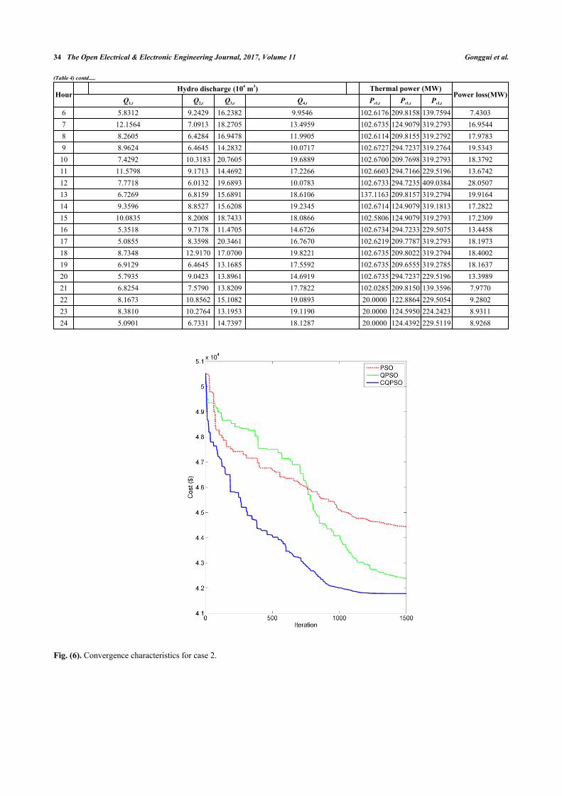
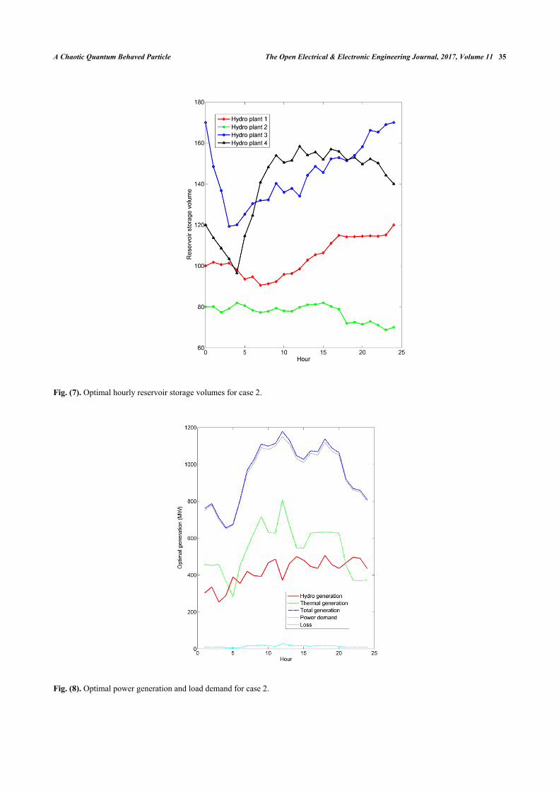
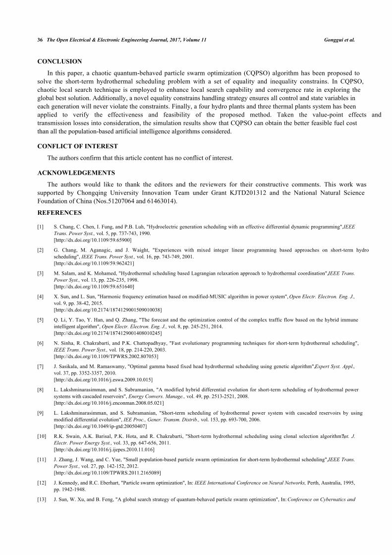
performance than QPSO and other method. Fig. (6) shows the convergence of PSO, QPSO and CQPSO for the trial runthat produced the minimum cost solution. The optimal hydro discharges, the optimal thermal generation, and the totaltransmission losses obtained by CQPSO accompany with the system power demand are demonstrated in Table 4. Thehourly reservoir storage volumes of four hydro plants are shown in Fig. (7). The Optimal hourly power generation,transmission losses and load demand are shown in Fig. (8). It is important to note that all control and state variablesremained within their permissible limits.

Fig. (5). Optimal power generation and load demand for case 1.

Table 3. Comparison of simulation results for case 2.

Method Minimum cost ($) Average cost ($) Maximum cost ($) CPU time (s)MHDE [8] 42679.87 - - 40

SPPSO [11] 42740.23 43622.14 44346.97 32.7PSO 44431.089 44711.496 45158.586 151.1

QPSO 42375.926 42971.683 43389.563 134.5CQPSO 41785.665 41972.366 42098.316 64.5

Table 4. Optimal hydro discharge, thermal generation and power loss for case 2.

HourHydro discharge (104 m3) Thermal power (MW)

Power loss(MW)Q1,t Q2,t Q3,t Q4,t Ps1,t Ps1,t Ps1,t

1 8.2245 7.9191 29.6237 9.1369 102.6595 124.7263 229.5104 10.50152 10.1855 10.7757 19.9313 7.4709 102.6561 209.6966 139.7385 7.48103 7.2637 7.1659 29.7072 6.7772 102.6509 124.9049 229.4984 10.42784 10.2128 6.2541 19.3666 6.9397 102.6533 124.8233 139.7579 6.17615 10.6099 9.3396 15.8075 11.5044 20.0000 124.3139 139.6987 4.4665

34 The Open Electrical & Electronic Engineering Journal, 2017, Volume 11 Gonggui et al.

HourHydro discharge (104 m3) Thermal power (MW)

Power loss(MW)Q1,t Q2,t Q3,t Q4,t Ps1,t Ps1,t Ps1,t

6 5.8312 9.2429 16.2382 9.9546 102.6176 209.8158 139.7594 7.43037 12.1564 7.0913 18.2705 13.4959 102.6735 124.9079 319.2793 16.95448 8.2605 6.4284 16.9478 11.9905 102.6114 209.8155 319.2792 17.97839 8.9624 6.4645 14.2832 10.0717 102.6727 294.7237 319.2764 19.534310 7.4292 10.3183 20.7605 19.6889 102.6700 209.7698 319.2793 18.379211 11.5798 9.1713 14.4692 17.2266 102.6603 294.7166 229.5196 13.674212 7.7718 6.0132 19.6893 10.0783 102.6733 294.7235 409.0384 28.050713 6.7269 6.8159 15.6891 18.6106 137.1163 209.8157 319.2794 19.916414 9.3596 8.8527 15.6208 19.2345 102.6714 124.9079 319.1813 17.282215 10.0835 8.2008 18.7433 18.0866 102.5806 124.9079 319.2793 17.230916 5.3518 9.7178 11.4705 14.6726 102.6734 294.7233 229.5075 13.445817 5.0855 8.3598 20.3461 16.7670 102.6219 209.7787 319.2793 18.197318 8.7348 12.9170 17.0700 19.8221 102.6735 209.8022 319.2794 18.400219 6.9129 6.4645 13.1685 17.5592 102.6735 209.6555 319.2785 18.163720 5.7935 9.0423 13.8961 14.6919 102.6735 294.7237 229.5196 13.398921 6.8254 7.5790 13.8209 17.7822 102.0285 209.8150 139.3596 7.977022 8.1673 10.8562 15.1082 19.0893 20.0000 122.8864 229.5054 9.280223 8.3810 10.2764 13.1953 19.1190 20.0000 124.5950 224.2423 8.931124 5.0901 6.7331 14.7397 18.1287 20.0000 124.4392 229.5119 8.9268

Fig. (6). Convergence characteristics for case 2.

(Table 4) contd.....

A Chaotic Quantum Behaved Particle The Open Electrical & Electronic Engineering Journal, 2017, Volume 11 35

Fig. (7). Optimal hourly reservoir storage volumes for case 2.

Fig. (8). Optimal power generation and load demand for case 2.

36 The Open Electrical & Electronic Engineering Journal, 2017, Volume 11 Gonggui et al.

CONCLUSION

In this paper, a chaotic quantum-behaved particle swarm optimization (CQPSO) algorithm has been proposed tosolve the short-term hydrothermal scheduling problem with a set of equality and inequality constrains. In CQPSO,chaotic local search technique is employed to enhance local search capability and convergence rate in exploring theglobal best solution. Additionally, a novel equality constrains handling strategy ensures all control and state variables ineach generation will never violate the constraints. Finally, a four hydro plants and three thermal plants system has beenapplied to verify the effectiveness and feasibility of the proposed method. Taken the value-point effects andtransmission losses into consideration, the simulation results show that CQPSO can obtain the better feasible fuel costthan all the population-based artificial intelligence algorithms considered.

CONFLICT OF INTEREST

The authors confirm that this article content has no conflict of interest.

ACKNOWLEDGEMENTS

The authors would like to thank the editors and the reviewers for their constructive comments. This work wassupported by Chongqing University Innovation Team under Grant KJTD201312 and the National Natural ScienceFoundation of China (Nos.51207064 and 61463014).

REFERENCES

[1] S. Chang, C. Chen, I. Fung, and P.B. Luh, "Hydroelectric generation scheduling with an effective differential dynamic programming", IEEETrans. Power Syst., vol. 5, pp. 737-743, 1990.[http://dx.doi.org/10.1109/59.65900]

[2] G. Chang, M. Aganagic, and J. Waight, "Experiences with mixed integer linear programming based approaches on short-term hydroscheduling", IEEE Trans. Power Syst., vol. 16, pp. 743-749, 2001.[http://dx.doi.org/10.1109/59.962421]

[3] M. Salam, and K. Mohamed, "Hydrothermal scheduling based Lagrangian relaxation approach to hydrothermal coordination", IEEE Trans.Power Syst., vol. 13, pp. 226-235, 1998.[http://dx.doi.org/10.1109/59.651640]

[4] X. Sun, and L. Sun, "Harmonic frequency estimation based on modified-MUSIC algorithm in power system", Open Electr. Electron. Eng. J.,vol. 9, pp. 38-42, 2015.[http://dx.doi.org/10.2174/1874129001509010038]

[5] Q. Li, Y. Tao, Y. Han, and Q. Zhang, "The forecast and the optimization control of the complex traffic flow based on the hybrid immuneintelligent algorithm", Open Electr. Electron. Eng. J., vol. 8, pp. 245-251, 2014.[http://dx.doi.org/10.2174/1874129001408010245]

[6] N. Sinha, R. Chakrabarti, and P.K. Chattopadhyay, "Fast evolutionary programming techniques for short-term hydrothermal scheduling",IEEE Trans. Power Syst., vol. 18, pp. 214-220, 2003.[http://dx.doi.org/10.1109/TPWRS.2002.807053]

[7] J. Sasikala, and M. Ramaswamy, "Optimal gamma based fixed head hydrothermal scheduling using genetic algorithm", Expert Syst. Appl.,vol. 37, pp. 3352-3357, 2010.[http://dx.doi.org/10.1016/j.eswa.2009.10.015]

[8] L. Lakshminarasimman, and S. Subramanian, "A modified hybrid differential evolution for short-term scheduling of hydrothermal powersystems with cascaded reservoirs", Energy Convers. Manage., vol. 49, pp. 2513-2521, 2008.[http://dx.doi.org/10.1016/j.enconman.2008.05.021]

[9] L. Lakshminarasimman, and S. Subramanian, "Short-term scheduling of hydrothermal power system with cascaded reservoirs by usingmodified differential evolution", IEE Proc., Gener. Transm. Distrib., vol. 153, pp. 693-700, 2006.[http://dx.doi.org/10.1049/ip-gtd:20050407]

[10] R.K. Swain, A.K. Barisal, P.K. Hota, and R. Chakrabarti, "Short-term hydrothermal scheduling using clonal selection algorithm", Int. J.Electr. Power Energy Syst., vol. 33, pp. 647-656, 2011.[http://dx.doi.org/10.1016/j.ijepes.2010.11.016]

[11] J. Zhang, J. Wang, and C. Yue, "Small population-based particle swarm optimization for short-term hydrothermal scheduling", IEEE Trans.Power Syst., vol. 27, pp. 142-152, 2012.[http://dx.doi.org/10.1109/TPWRS.2011.2165089]

[12] J. Kennedy, and R.C. Eberhart, "Particle swarm optimization", In: IEEE International Conference on Neural Networks, Perth, Australia, 1995,pp. 1942-1948.

[13] J. Sun, W. Xu, and B. Feng, "A global search strategy of quantum-behaved particle swarm optimization", In: Conference on Cybernatics and

A Chaotic Quantum Behaved Particle The Open Electrical & Electronic Engineering Journal, 2017, Volume 11 37

intelligent Systems, Singapore, 2004.

[14] O.E. Turgut, M.S. Turgut, and M.T. Coban, "Chaotic quantum behaved particle swarm optimization algorithm for solving nonlinear system ofequations", Comput. Math. Appl., vol. 68, pp. 508-530, 2014.[http://dx.doi.org/10.1016/j.camwa.2014.06.013]

[15] M. Clerc, and J. Kennedy, "The particle swarm - explosion, stability, and convergence in a multidimensional complex space", IEEE Trans.Evol. Comput., vol. 6, pp. 58-73, 2002.[http://dx.doi.org/10.1109/4235.985692]

[16] Coelho and L. D. Santos, "A quantum particle swarm optimizer with chaotic mutation operator", Chaos Solitons Fractals, vol. 37, pp.1409-1418, 2008.[http://dx.doi.org/10.1016/j.chaos.2006.10.028]

[17] Coelho and L. D. Santos, "Gaussian quantum-behaved particle swarm optimization approaches for constrained engineering design problems",Expert Syst. Appl., vol. 37, pp. 1676-1683, 2010.[http://dx.doi.org/10.1016/j.eswa.2009.06.044]

[18] O.E. Turgut, "Hybrid Chaotic Quantum behaved Particle Swarm Optimization algorithm for thermal design of plate fin heat exchangers",Appl. Math. Model., vol. 29, pp. 298-309, 2015.

[19] R.M. May, "Simple mathematical models with very complicated dynamics", Nature., vol. 261, no. 5560, pp. 459-467, 1976.[http://dx.doi.org/10.1038/261459a0] [PMID: 934280]

[20] Y. Lu, J. Zhou, H. Qin, Y. Wang, and Y. Zhang, "An adaptive chaotic differential evolution for the short-term hydrothermal generationscheduling problem", Energy Convers. Manage., vol. 51, pp. 1481-1490, 2010.[http://dx.doi.org/10.1016/j.enconman.2010.02.006]

[21] X. Yuan, B. Cao, B. Yang, and Y. Yuan, "Hydrothermal scheduling using chaotic hybrid differential evolution", Energy Convers. Manage.,vol. 49, pp. 3627-3633, 2008.[http://dx.doi.org/10.1016/j.enconman.2008.07.008]

[22] P. Kumar Roy, A. Sur, and D.K. Pradhan, "Optimal short-term hydro-thermal scheduling using quasi-oppositional teaching learning basedoptimization", Eng. Appl. Artif. Intell., vol. 26, pp. 2516-2524, 2013.[http://dx.doi.org/10.1016/j.engappai.2013.08.002]

[23] J. Zhang, J. Wang, and C. Yue, "Small population-based particle swarm optimization for short-term hydrothermal scheduling", IEEE Trans.Power Syst., vol. 27, pp. 142-152, 2012.[http://dx.doi.org/10.1109/TPWRS.2011.2165089]

© Gonggui et al.; Licensee Bentham Open

This is an open access article licensed under the terms of the Creative Commons Attribution-Non-Commercial 4.0 International Public License(CC BY-NC 4.0) (https://creativecommons.org/licenses/by-nc/4.0/legalcode), which permits unrestricted, non-commercial use, distribution andreproduction in any medium, provided the work is properly cited.