a case study on the effects of …flux.aos.wisc.edu/~adesai/documents/desai-blm-part1.pdf · loon...
TRANSCRIPT

DOI 10.1007/s10546-005-9024-6Boundary-Layer Meteorology (2006) 119: 195–238 © Springer 2005
A CASE STUDY ON THE EFFECTS OF HETEROGENEOUS SOILMOISTURE ON MESOSCALE BOUNDARY-LAYER STRUCTURE
IN THE SOUTHERN GREAT PLAINS, U.S.A. PART I: SIMPLEPROGNOSTIC MODEL
ANKUR R. DESAI1,∗, KENNETH J. DAVIS1, CHRISTOPH J. SENFF2,SYED ISMAIL3, EDWARD V. BROWELL3, DAVID R. STAUFFER1
and BRIAN P. REEN1
1Department of Meteorology, The Pennsylvania State University, 503 Walker Building,University Park, PA 16802, U.S.A.; 2Atmospheric Lidar Division, NOAA Environmental
Technology Laboratory, Boulder, CO, U.S.A.; 3Atmospheric Sciences Division, NASALangley Research Center, Hampton, VA, U.S.A.
(Received in final form 15 August 2005 / Published online: 17 December 2005)
Abstract. The atmospheric boundary-layer (ABL) depth was observed by airborne lidar andballoon soundings during the Southern Great Plains 1997 field study (SGP97). This paperis Part I of a two-part case study examining the relationship of surface heterogeneity toobserved ABL structure. Part I focuses on observations. During two days (12–13 July 1997)following rain, midday convective ABL depth varied by as much as 1.5 km across 400 km,even with moderate winds. Variability in ABL depth was driven primarily by the spatial vari-ation in surface buoyancy flux as measured from short towers and aircraft within the SGP97domain. Strong correlation was found between time-integrated buoyancy flux and airborneremotely sensed surface soil moisture for the two case-study days, but only a weak correla-tion was found between surface energy fluxes and vegetation greenness as measured by satel-lite. A simple prognostic one-dimensional ABL model was applied to test to what extent thesoil moisture spatial heterogeneity explained the variation in north–south ABL depth acrossthe SGP97 domain. The model was able to better predict mean ABL depth and variationson horizontal scales of approximately 100 km using observed soil moisture instead of con-stant soil moisture. Subsidence, advection, convergence/divergence and spatial variability oftemperature inversion strength also contributed to ABL depth variations. In Part II, assim-ilation of high-resolution soil moisture into a three-dimensional mesoscale model (MM5) isdiscussed and shown to improve predictions of ABL structure. These results have implica-tions for ABL models and the influence of soil moisture on mesoscale meteorology.
Keywords: Boundary-layer depth, Convective boundary layer, Lidar, Soil moisture, Surfacebuoyancy flux.
* E-mail: [email protected]

196 ANKUR R. DESAI ET AL.
1. Introduction
Spatial and temporal evolution in the depth of mixing in the atmosphericboundary layer (ABL) can have a profound influence on local weatherand cloud cover. The causes of mesoscale (tens to hundreds of km) vari-ations in the ABL depth are not well understood but have been shownto be mediated by surface heterogeneity (Mahrt, 2000). We present a casestudy of observed mesoscale ABL variations on 12 and 13 July 1997 acrossthe Southern Great Plains region of Oklahoma and Kansas, U.S.A. Bal-loon sounding and lidar observed ABL depth varied by as much as 1.5 kmacross 400 km on 12 July but only varied less than 0.5 km on 13 July. Bothdays had clear to partly-cloudy weather following rain on 10–11 July andmidday ABL wind speeds of 7–10 m s−1 (Table I).
The observed variations in mesoscale ABL depth cannot be explainedby larger scale boundaries such as fronts or drylines since none were evi-dent on the two anticyclonic dominated days. Previous work in the South-ern Great Plains has shown that ABL depth as examined from balloonsoundings varied by a factor of 3 and was driven mostly by variabilityin surface energy fluxes (Hubbe et al., 1997). Thus, we hypothesized thatmesoscale ABL depth variability on the two case study days was alsodriven by the variability in surface energy fluxes.
Surface energy fluxes measured from short towers can be highly variableacross the landscape since they are a function of local vegetation, soil type,soil moisture, micrometeorological processes and fetch. However, mesoscalespatial patterns in surface energy fluxes observed from many towers areindicative of mesoscale variations in surface properties or meteorology. Var-iability in surface energy flux has an impact on cloud cover, convective ini-tiation, rainfall intensity and atmospheric stability (Yan and Anthes, 1988;Avissar and Pielke, 1989; Zhong and Doran, 1997; Avissar and Schmidt,1998). Vegetation cover and surface water availability appear to be pri-mary factors that explain large-scale patterns in surface fluxes, especiallyin sparsely vegetated areas (Dirmeyer et al., 2000; Betts, 2004), and vari-ations in surface parameters and surface fluxes have been shown to gener-ate mesoscale boundary-layer circulations (Segal and Arritt, 1992; Weaver,2004). Climate models suggest that the Southern Great Plains is a regionwhere soil moisture is strongly coupled to precipitation patterns (Kosteret al., 2004) and ABL structure (Betts and Ball, 1996). Thus, we hypothe-size that surface soil moisture can explain the mesoscale variability in sur-face energy flux, and consequently, ABL depth, since 12 and 13 July werepreceded by rain on July 10 and 11.
These hypotheses are not necessarily new or surprising. But while the-oretical and modelling work on surface flux and ABL evolution has beendone, observational studies at this scale and with a large matrix of instruments

ABL DEPTH VARIABILITY DURING SGP97 197
TA
BL
EI
Wea
ther
cond
itio
nsdu
ring
the
case
stud
yat
the
AR
M-C
AR
TC
entr
alF
acili
ty.
Wat
erva
pour
Mea
nte
mp.
Max
.te
mp.
Min
.te
mp.
Pre
ssur
eP
reci
pm
ixin
gra
tio
Win
dsp
eed
atW
ind
dire
ctio
nD
ate
at2
m(◦ C
)(◦ C
)(◦ C
)(h
Pa)
(mm
)(g
kg−1
)10
m(m
s−1)
(deg
rees
)
10Ju
ly97
2633
2297
79
16.1
615
511
July
9725
3121
977
517
.66.
115
212
July
9728
3423
977
016
.48.
116
813
July
9729
3623
975
016
.27.
217
3

198 ANKUR R. DESAI ET AL.
are uncommon. High spatial resolution and frequent temporal observationsof ABL depth, surface energy fluxes, soil moisture, and surface vegetativeproperties are rare and not a part of routine observations. The SouthernGreat Plains 1997 (SGP97) hydrology experiment (Jackson, 1997) was oneof few studies that included a large array of observations to allow for anexamination of the causes of mesoscale ABL depth variability.
The objective of this study was to examine the causes of spatial variabilityin ABL development across the SGP97 area and to test new tools for study-ing this variability. To accomplish this objective, we explore the relationshipbetween two land-cover variables and surface energy flux and develop a sim-ple ABL model to examine the impact of surface forcing heterogeneity onABL depth. We have chosen to use an empirical model tuned to the regionand time period in order to maximize the combination of spatial resolutionand areal coverage, and to test a unique remote sensing data source.
The two surface remote sensing instruments used in this study are theU.S. National Oceanic and Atmospheric Administration (NOAA) AdvancedVery High-Frequency Radiometer (AVHRR) and the Electronically ScannedThinned Array Radiometer (ESTAR), and their two respective land-covermeasurements are vegetation cover and surface soil moisture. ESTAR isa passive microwave-based remote sensing system (Le Vine et al., 1994)that was flown on the U.S. National Aeronautics and Space Administra-tion (NASA) P-3 aircraft across the SGP97 study area for several days tovalidate ESTAR operation and soil moisture retrieval algorithms (Jacksonet al., 1999). Along with ESTAR, NASA Langley’s Lidar Atmospheric Sens-ing Experiment (LASE) was flown on the P-3 to measure high vertical resolu-tion aerosol scattering ratio and water vapour profiles using the DifferentialAbsorption Lidar (DIAL) technique (Browell et al., 1997). High-resolutionABL depth measurements were derived from the LASE data.
The primary questions we asked in this study were: (1) Was there anycorrelation between the observed mesoscale ABL depth spatial variabilityand surface energy flux variability? (2) Was there any correlation betweenmesoscale surface flux variability and surface parameters? and (3) At whatscale did surface parameters appear to influence ABL depth variability?In this study, we examined observed ABL depth from balloon sound-ings and airplane-mounted lidar during the drying period. We comparedthese depths to observations of integrated surface buoyancy flux mea-sured at surface energy flux stations. We also compared energy fluxes toremotely-sensed measurements of soil moisture and vegetation. A simpleone-dimensional (1-D) ABL model was developed and applied to furtherunderstand to what extent and scale did surface properties explain observedABL depth. Part II of this study examines the influence of assimilatinghigh resolution soil moisture into a full three-dimensional (3-D) mesoscalemodel (Reen et al., submitted).

ABL DEPTH VARIABILITY DURING SGP97 199
2. Case Study Description
2.1. Southern great plains 1997 study
The Southern Great Plains 1997 field study occurred during late spring andsummer of 1997 over northern Oklahoma and southern Kansas, U.S.A.(Figure 1). The area can be characterized as sub-humid grasslands withflat to moderately rolling terrain and a maximum relief of less than 200 m.Grassland and winter wheat are the dominant land-use types (Jacksonet al., 1999). Local standard time (LST) is UTC – 6 hours.
The primary goal of SGP97 was validation of the soil moisture retrievalalgorithms of ESTAR, which has been previously shown with in-situ databy Jackson et al. (1999) and also by comparison with a mesoscale modeldriven with an offline land-surface model (Reen et al., submitted). An addi-tional objective was to examine the effect of soil moisture on the evolu-tion of the ABL and clouds over the Southern Great Plains. In additionto the LASE and ESTAR, data were also collected by the U.S. Departmentof Energy (DOE) Atmospheric Radiation Measurement Cloud and Radia-tion Testbed (ARM-CART) flux and balloon sounding facilities, OklahomaMesonet weather stations, two aircraft equipped to measure surface energyfluxes and SGP97 flux towers set up by the U.S. Department of Agricul-ture Agricultural Research Service (USDA ARS), University of Wisconsin– Madison, the NASA Jet Propulsion Laboratory, Georgia Tech, NOAAAtmospheric Turbulence and Diffusion Division (ATDD) and the Universityof Arizona. ESTAR and LASE observations from 12 to 13 July are centralto this study. Additional site information and data access are available athttp://www.arm.gov/sites/sgp.stm, http://disc.gsfc.nasa.gov/fieldexp/SGP97/,and http://hydrolab.arsusda.gov/sgp97.
2.2. Case study conditions
Conditions prior and during the case study observed at the ARM-CARTCentral Facility Surface Meteorological Observation System consisted ofwarm, moist conditions with moderate southerly and south-easterly winds(Table I). Precipitation fell from 8 July through 11 July, primarily on10 July (MacPherson, 1998). There was a strong north–south precipita-tion gradient across the measurement domain as observed by precipita-tion measurement sites included in the Global Energy and Water CycleExperiment (GEWEX) daily precipitation composite (Figure 2). Total pre-cipitation from 8 to 12 July, averaged across 1 degree latitude bands withinthe roughly 400 km SGP97 domain, varied from less than 5 mm in thesouth to greater than 50 mm in the north. This variability in antecedent

200 ANKUR R. DESAI ET AL.
Kansas
Oklahoma
Oklahoma
Texas
Red River
Canadian River
Ark
ansas River
El Reno Oklahoma City
Lawton
Ada
Enid
Wichita
Arkansas City
Norman
Salina
Hutchinson
34
35
36
37
38
9596979899100
40
40
35
35
70 70
44
44
NLine G
Line B
Line D
Line E
Line R
Projection: UTM Zone 14
Sonde site
ARM-CART Bowen ratio flux system site
ARM-CART eddy covariance flux system site
SGP97 researcher flux site
ESTAR / LASE coverage 12 July 1997
AVHRR-14 coverage 12 July 1997
Legend
B5
B4
C1
B1
B6
0 100 200
Kilometers
39
Central Facility
(Lamont)
Figure 1. Map of Southern Great Plains 1997 study area and measurement site locations.NDVI (grey box) and ESTAR (white box) coverage on 12 July is also noted.

ABL DEPTH VARIABILITY DURING SGP97 201
34.5 35.0 35.5 36.0 36.5 37.0 37.5 38.0 38.5
Latitude (degrees N)
0
10
20
30
40
50
Tot
al P
reci
pita
tion
(mm
)
8-12 July 1997
96.5° W to 98.5° W longitude
Figure 2. Observed total precipitation from 8 to 12 July 1997 averaged across 1 degree latitudebands centred on the latitudes shown and with longitude ranging from 96.5◦ W to 98.5◦ W.
precipitation was the primary cause in observed variation in surface soilmoisture on 12 and 13 July.
3. Observations
Our primary goal was to examine the spatial variability of ABL depthand relate it to variability in surface energy fluxes and surface parame-ters. Point-based estimates of ABL depth were based on ARM-CART bal-loon soundings. North–south tracks of observed ABL depth were derivedfrom the LASE aerosol data. Remotely-sensed surface soil moisture, aremotely sensed vegetation index and a spatially distributed set of tempo-rally continuous measurements of surface energy flux were used to correlatepoint-based flux measurements to spatial maps of soil moisture and vege-tation cover. These data came respectively from airplane-mounted ESTAR,NOAA AVHRR, and various tower-based flux stations spread across theSGP97 area. Energy fluxes were also observed from aircraft in variousparts of the SGP97 area. For SGP97, clear, sunny days and the availabil-ity of ESTAR, AVHRR, LASE and a full suite of flux data coincided on12–13 July, during the drying period after prior rainfall.

202 ANKUR R. DESAI ET AL.
3.1. Soundings
ARM-CART Balloon-Borne Sounding System (BBSS) balloon soundingswere launched once every 3 hours from five locations during the study timeframe (Table II and Figure 1). One balloon sounding was located whollywithin the ESTAR region on both days. Balloon sounding output was usedin this study to compute potential temperature profiles and visually esti-mate ABL depth from these profiles. Balloon sounding wind speed anddirection were used for advection and subsidence calculations. Vertical res-olution was approximately 10 m, and ABL depth was chosen visually to thenearest 25 m with ± 50 m accuracy. Additional information about the BBSSsystem is at http://www.arm.gov/instruments/instrument.php?id=6.
3.2. Lidar
The LASE system was developed at the NASA Langley Research Centerto measure atmospheric water vapour profiles, aerosol profiles and clouddistributions from aircraft (Browell et al., 1997). LASE is a compactand highly engineered differential absorption lidar system that has dem-onstrated autonomous operation from the high-altitude ER-2 aircraft asa precursor to the development of a space-borne DIAL system. DuringSGP97, LASE was reconfigured and operated in the nadir mode from theNASA P-3 aircraft. The laser system consists of a double-pulsed Ti:sap-phire laser that operates in the 815 nm absorption band of water vapourand is pumped by a frequency doubled Nd:YAG laser. The double pulsingis needed to generate the on and off line pair needed for the DIAL watervapour measurements (Browell, 1989). The on and off lines are spectrallypositioned on the water vapour absorption line so that there is insignificantabsorption at the off line and optimum absorption at the on line due to thepresence of water vapour in the atmosphere.
Lidar measurements at the off line were used to derive aerosol back-scattering profiles. The off line lidar signals were background subtractedand range corrected (by multiplying by the square of the range) to derivethe relative atmospheric backscattering profiles. The relative backscatteringprofiles can be used to obtain ABL properties (Ismail et al., 1998). Aer-osol backscatter profiles from the LASE were used to derive ABL depthvariations with high spatial resolution (Davis et al., 2000). Resolution was150 m in the horizontal and the vertical range gate was 30 m. ABL depthwas computed using a stepped wavelet function with a 250-m dilation scale.Further details on LASE are available at http://asd-www.larc.nasa.gov/lidar/lidar.html and http://asd-www.larc.nasa.gov/lidar/sgp97/sgp97.html. Thisstudy focused on late morning and midday north–south P-3 tracks on 12and 13 July.

ABL DEPTH VARIABILITY DURING SGP97 203
TA
BL
EII
AR
Mba
lloon
-bor
neso
undi
ngsy
stem
sin
the
SGP
97re
gion
.
z iz i
z iz i
z iz i
12dT
/dz
0830
1130
1430
13dθ v
/dz
0830
1130
1430
Stat
ion
Reg
ion
Loc
atio
nL
atit
ude
Lon
gitu
deJu
ly(K
km−1
)L
ST(m
)L
ST(m
)L
ST(m
)Ju
ly(K
km−1
)L
ST(m
)L
ST(m
)L
ST(m
)
B1
Nor
thH
illsb
oro,
38◦ 1
8′00
"97
◦ 18′
00"
10.9
625
875
1225
14.0
475
700
1400
KS
C1
Cen
tral
Lam
ont,
36◦ 3
6′36
"97
◦ 29′
24"
10.5
650
1100
1975
18.4
475
1125
975
OK
B6
Sout
hP
urce
ll,34
◦ 57′
36"
97◦ 2
5′12
"10
.821
7513
.055
010
0018
25O
KB
4W
est
Vic
i,O
K36
◦ 04′
12"
99◦ 1
2′00
"12
.435
067
580
016
.245
065
010
00B
5E
ast
Mor
ris,
OK
35◦ 4
0′48
"95
◦ 51′
00"
8.5
475
850
1075
12.4
450
975
925
dθv/d
zis
the
incr
ease
invi
rtua
lpo
tent
ial
tem
pera
ture
ofea
rly
mor
ning
soun
ding
s(0
530
LST
)be
twee
n0
and
500
m.

204 ANKUR R. DESAI ET AL.
3.3. Estar
ESTAR was designed as a passive microwave remote sensor to be usedin space for global soil moisture mapping at relatively coarse resolutions(10–30 km) (Le Vine et al., 1994). Surface (< 50 mm) soil moisture hasbeen shown to be related to passive microwave brightness temperature(USDA ARS, cited 1997: Southern Great Plains 1997 hydrology experimentplan [Available online at http://hydrolab.arsusda.gov/sgp97/explan/]). DuringSGP97, ESTAR was operated at a nominal altitude of 7.5 km from theNASA Wallops Flight Facilities’ P-3B aircraft.
Information from ESTAR was gridded to produce a map of micro-wave ground reflectance across and along the airplane track at 400-mresolution. Soil moisture from ESTAR was computed from this bright-ness temperature map and the Fresnel reflectance inverse model equationfor horizontal polarization (Jackson et al., 1999). Inputs to this modelincluded microwave brightness temperature, soil temperature, vegetationtype, vegetation water content, surface roughness, soil bulk density andsoil texture. Model inputs were derived from Oklahoma Mesonet weatherstations and LandSat Thematic Mapper (TM) land-cover data. The out-put soil moisture map was gridded to 800-m resolution. The average errorin soil moisture compared to Oklahoma Mesonet observed soil moisturewas 3% (Jackson et al., 1999). More information and data are available athttp://disc.gsfc.nasa.gov/fieldexp/SGP97/estar.html.
3.4. Avhrr
NOAA AVHRR satellites produce visible and infrared images of theEarth’s surface at regular intervals at a 1.1-km resolution in the green, redand infrared bands. The Normalized Difference Vegetation Index (NDVI),a standard measure of vegetative cover, is calculated as the ratio of thedifference over the sum of the visible red and near infrared bands (Averyand Berlin, 1992). AVHRR NDVI data for the SGP97 region were avail-able in the morning, afternoon and evening of 12 July and the morningand afternoon of 13 July. In this study, afternoon NDVI data were usedfrom the NOAA-12 satellite.
In general, NDVI values range from −1 to 1, with typical NDVI val-ues for vegetated areas around 0.6, and only marginal increases in NDVIwith increasing vegetation cover after that threshold (Gillies and Carlson,1995). NDVI is often used as a proxy measure for leaf area index (LAI)(Chehbouni et al., 1997).
ABL DEPTH VARIABILITY DURING SGP97 205
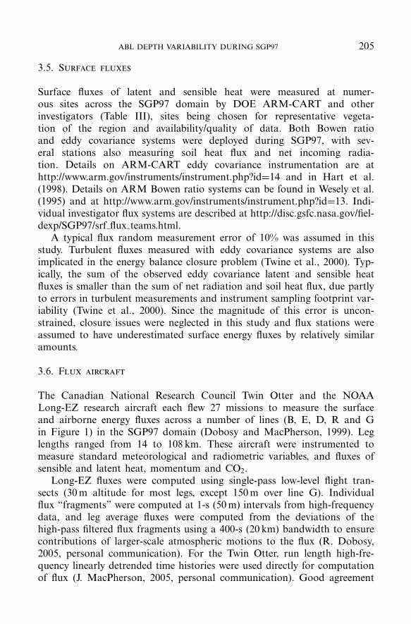
3.5. Surface fluxes
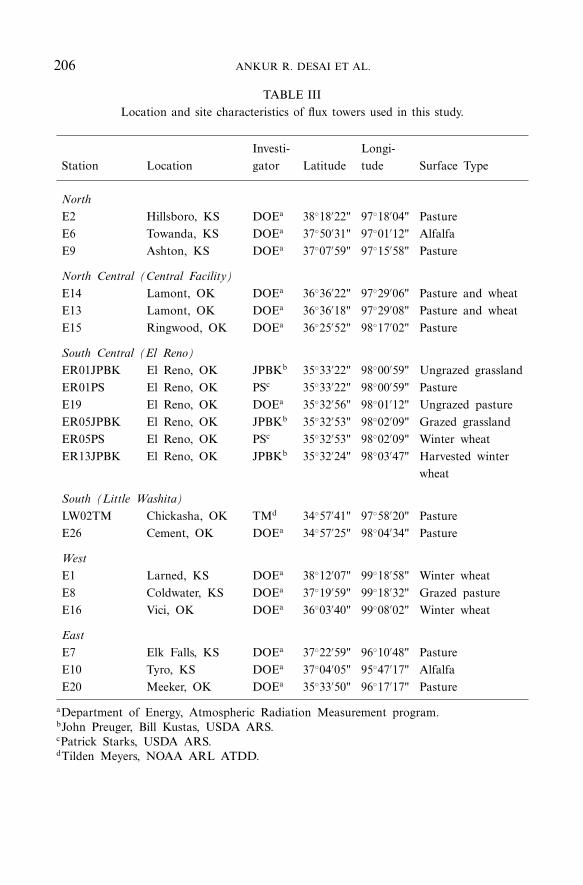
Surface fluxes of latent and sensible heat were measured at numer-ous sites across the SGP97 domain by DOE ARM-CART and otherinvestigators (Table III), sites being chosen for representative vegeta-tion of the region and availability/quality of data. Both Bowen ratioand eddy covariance systems were deployed during SGP97, with sev-eral stations also measuring soil heat flux and net incoming radia-tion. Details on ARM-CART eddy covariance instrumentation are athttp://www.arm.gov/instruments/instrument.php?id=14 and in Hart et al.(1998). Details on ARM Bowen ratio systems can be found in Wesely et al.(1995) and at http://www.arm.gov/instruments/instrument.php?id=13. Indi-vidual investigator flux systems are described at http://disc.gsfc.nasa.gov/fiel-dexp/SGP97/srf flux teams.html.
A typical flux random measurement error of 10% was assumed in thisstudy. Turbulent fluxes measured with eddy covariance systems are alsoimplicated in the energy balance closure problem (Twine et al., 2000). Typ-ically, the sum of the observed eddy covariance latent and sensible heatfluxes is smaller than the sum of net radiation and soil heat flux, due partlyto errors in turbulent measurements and instrument sampling footprint var-iability (Twine et al., 2000). Since the magnitude of this error is uncon-strained, closure issues were neglected in this study and flux stations wereassumed to have underestimated surface energy fluxes by relatively similaramounts.
3.6. Flux aircraft
The Canadian National Research Council Twin Otter and the NOAALong-EZ research aircraft each flew 27 missions to measure the surfaceand airborne energy fluxes across a number of lines (B, E, D, R and Gin Figure 1) in the SGP97 domain (Dobosy and MacPherson, 1999). Leglengths ranged from 14 to 108 km. These aircraft were instrumented tomeasure standard meteorological and radiometric variables, and fluxes ofsensible and latent heat, momentum and CO2.
Long-EZ fluxes were computed using single-pass low-level flight tran-sects (30 m altitude for most legs, except 150 m over line G). Individualflux “fragments” were computed at 1-s (50 m) intervals from high-frequencydata, and leg average fluxes were computed from the deviations of thehigh-pass filtered flux fragments using a 400-s (20 km) bandwidth to ensurecontributions of larger-scale atmospheric motions to the flux (R. Dobosy,2005, personal communication). For the Twin Otter, run length high-fre-quency linearly detrended time histories were used directly for computationof flux (J. MacPherson, 2005, personal communication). Good agreement
206 ANKUR R. DESAI ET AL.
TABLE III
Location and site characteristics of flux towers used in this study.
Investi- Longi-Station Location gator Latitude tude Surface Type
North
E2 Hillsboro, KS DOEa 38◦18′22" 97◦18′04" PastureE6 Towanda, KS DOEa 37◦50′31" 97◦01′12" AlfalfaE9 Ashton, KS DOEa 37◦07′59" 97◦15′58" Pasture
North Central (Central Facility)
E14 Lamont, OK DOEa 36◦36′22" 97◦29′06" Pasture and wheatE13 Lamont, OK DOEa 36◦36′18" 97◦29′08" Pasture and wheatE15 Ringwood, OK DOEa 36◦25′52" 98◦17′02" Pasture
South Central (El Reno)
ER01JPBK El Reno, OK JPBKb 35◦33′22" 98◦00′59" Ungrazed grasslandER01PS El Reno, OK PSc 35◦33′22" 98◦00′59" PastureE19 El Reno, OK DOEa 35◦32′56" 98◦01′12" Ungrazed pastureER05JPBK El Reno, OK JPBKb 35◦32′53" 98◦02′09" Grazed grasslandER05PS El Reno, OK PSc 35◦32′53" 98◦02′09" Winter wheatER13JPBK El Reno, OK JPBKb 35◦32′24" 98◦03′47" Harvested winter
wheat
South (Little Washita)
LW02TM Chickasha, OK TMd 34◦57′41" 97◦58′20" PastureE26 Cement, OK DOEa 34◦57′25" 98◦04′34" Pasture
West
E1 Larned, KS DOEa 38◦12′07" 99◦18′58" Winter wheatE8 Coldwater, KS DOEa 37◦19′59" 99◦18′32" Grazed pastureE16 Vici, OK DOEa 36◦03′40" 99◦08′02" Winter wheat
East
E7 Elk Falls, KS DOEa 37◦22′59" 96◦10′48" PastureE10 Tyro, KS DOEa 37◦04′05" 95◦47′17" AlfalfaE20 Meeker, OK DOEa 35◦33′50" 96◦17′17" Pasture
aDepartment of Energy, Atmospheric Radiation Measurement program.bJohn Preuger, Bill Kustas, USDA ARS.cPatrick Starks, USDA ARS.dTilden Meyers, NOAA ARL ATDD.

ABL DEPTH VARIABILITY DURING SGP97 207
was found among Long-EZ, Twin Otter and tower measured fluxes dur-ing concurrent passes on prior SGP97 missions (R. Dobosy, 2005, personalcommunication).
Line average fluxes were used in this case study. Shorter line fragmentswere not studied due to issues related to inherent turbulent sampling var-iability with aircraft measured fluxes (LeMone et al., 2003). Flux uncer-tainty was estimated to be approximately 20% (Mann and Lenschow, 1994).More information on these flights and flux processing details can be foundat http://disc.gsfc.nasa.gov/fieldexp/SGP97/air boundary.html.
4. Methods
4.1. Surface parameters and correlations to buoyancy flux
Surface energy fluxes observed from short towers and aircraft were exam-ined for spatial correlation with surface parameters and ABL depth. Sinceour goal was to examine the effect of total surface forcing on midday ABLdepth, and since observed latent heat fluxes were larger than sensible heatfluxes on both days, we examined time integrated surface buoyancy fluxfrom morning (0530 LST) to afternoon (1230 LST):
F =∫ t1
t0
(w′θ ′
v
)sdt, (1)
where surface buoyancy flux (K m s−1) was calculated from observed sur-face energy fluxes as
w′θ ′v = H
ρcp
+0.61θ
(L
ρdLv
)(2)
and where H is sensible heat flux (W m−2) and L is latent heat flux(W m−2).
The construction of a quantitative relation between remotely sensed veg-etation greenness or soil moisture to surface buoyancy flux required regis-tration of point locations of flux towers to the gridded surface parameterdata. Since fluxes measured from small towers (<10 m high) tend to have afootprints that extend about 100–2000 m upwind (Pelgrum and Bastiaanssen,1996), we averaged surface parameters for two pixels (1.6 km for ESTARand 2.2 km for AVHRR) in the upwind direction for each site. Errors aris-ing from the misalignment of station coordinates onto the surface parametergrids were considered by calculating a 3 × 3 pixel standard deviation of thesurface parameter for each station coordinate and including this as an errorto the assigned value of the surface parameter for that station.

208 ANKUR R. DESAI ET AL.
Time integrated buoyancy flux from 0530 to 1230 LST was com-pared to soil moisture and vegetation cover, and linear correlations werecreated between surface parameters and total forcing for both 12 and13 July and for ESTAR soil moisture and AVHRR NDVI. Regressionwas performed using the Fitexy algorithm (information at: http://idlas-tro.gsfc.nasa.gov/ftp/pro/math/fitexy.pro), a linear least squares regressionmethod that can account for errors both in the surface parameter (dueto instrument validation and misalignment error) and surface forcing (10%uncertainty). The fits were modified at the tails to prevent the net forc-ing from exceeding mean observed total available energy (net radiation −soil heat flux) and from falling below the lowest observed surface buoyancyflux.
We tested the reliability of a strong fit found between soil moisture andF by comparing soil moisture modelled buoyancy flux to airplane observedleg average flux. Soil moisture values along airplane legs were extractedfrom ESTAR soil moisture pixels 5 km upwind of the leg to account forflux footprint and advection as recommended by Song and Wesely (2003).Time varying modelled surface buoyancy flux was computed using a sinu-soidal model:
(w′θ ′
v
)s= (π
2 )F
3600 (t1 − t0)sin
( π2 (t − t0)
t1 − t0
), (3)
where t is time in hours, F is modelled from the relationship betweenESTAR soil moisture and observed tower-based surface fluxes, and t0 andt1 are the limits of integration in Equation (1).
4.2. ABL model
The correlation of soil moisture to surface buoyancy flux, soil moisturetransects derived from ESTAR, early morning virtual potential temperatureprofiles, and an ABL model were used to model ABL depth along the north–south P-3 track. A model for convective boundary-layer growth in responseto heterogeneous surface forcing was developed by Gryning and Batchvar-ova (1996) based on the encroachment models derived in Batchvarova andGryning (1991), Carson (1973) and Tennekes (1973):
{z2i
(1+2A)zi −2BκL+ Cu2
∗Tγg(1+A)zi −BκL
}(∂zi
∂t+u
∂zi
∂x+v
∂zi
∂y−ws
)
=(w′θ ′
v
)s
γ, (4)
where zi is mixed-layer depth, κ is the von Karman constant (0.4), L isthe Obhukhov length, u∗ is friction velocity, u and v are the along-track

ABL DEPTH VARIABILITY DURING SGP97 209
and across-track mean mixed-layer wind speed components, ws is subsi-dence rate, T is near-surface air temperature, g is gravity, γ is the virtualpotential temperature gradient above zi , and A,B and C are parameteriza-tion constants.
Batchvarova and Gryning (1991) show that terms related to mechanicalturbulence and ‘spin-up’ are only important when the mixed-layer depth issmall (e.g., early morning). Since our goal was to evaluate midday mixed-layer depth variability, and observed sounding data showed minimal varia-tion of zi in the morning, we neglect these terms and instead initialize themodel at mid-morning (0830 LST) with constant zi . Additionally, since wewere attempting to model observed ABL depth across the north–south P-3track and the wind direction on both days was nearly parallel to the track,we neglect across-track advection and instead average soil moisture data for15 km (1 m s−1 for 4-hour model period) upwind in the crosswind directionas a proxy for across-track advection. Equation (4) can then be simplifiedand rearranged to
∂zi
∂t= (1+2A)
(w′θ ′
v
)s
ziγ︸ ︷︷ ︸(a)
−∂uzi
∂x︸ ︷︷ ︸(b)
+ ws︸︷︷︸(c)
, (5)
where A is typically assumed to be 0.2 (Tennekes, 1973) and u and x are inthe direction of the P-3 track. Unlike Equation (4), we have also includedin term b of Equation (5) the effect of convergence/divergence on ABLdepth due to the spatial variation in wind velocity.
This simple model treats the convective boundary layer as a shallowwell-mixed 1-D fluid moving with the mean wind. ABL growth in thismodel is controlled by three terms: (a) a local forcing that encroaches uponthe mixed-layer inversion above zi , (b) a combined zi advection and local-scale convergence/divergence term, and (c) a net large-scale lifting/subsi-dence term. Entrainment flux at the top of the ABL is parameterized as aconstant fraction of surface buoyancy flux; shear-driven mixing, cross-trackadvection, and boundary-layer dynamics are ignored. These effects are bet-ter simulated with a 3-D mesoscale model, whose application is discussedin Part II of this paper (Reen et al., submitted). The modelling approachused here is admittedly simplistic, but provides an easy way to model andanalyze ABL depth using solely observed data in the region and a minimalnumber of assumptions.
We numerically solved Equation (5) along the north–south 413 km P-3track on 12 July and the 286 km P-3 track on 13 July with 1000 m hor-izontal resolution and a 30-s time step. The model was run from 0830 to1230 LST, and the 0830 LST initial ABL depth was set to a constant valuealong the track based on balloon soundings near the track (650 m on 12

210 ANKUR R. DESAI ET AL.
July and 500 m on 13 July). The equation was numerically solved at eachgrid point and time step using a second-order Lax-Wendroff explicit differ-ential scheme (Garcia, 2000). Each model run required 2–5 minutes of com-putation time on a standard desktop computer.
Time and space varying surface buoyancy flux was estimated using theregression of F to ESTAR soil moisture and Equation (3). Soil mois-ture to the north and south of the ESTAR domain was assumed to beconstant and equal to the northernmost or southernmost observed soilmoisture values, respectively. Along-track wind speeds (u) were calculatedby interpolation (inverse distance) of balloon sounding along-track windspeeds. Temperature gradient at the mixed-layer height was also calculatedby spatial interpolation of early morning (0530 LST) virtual potential tem-perature balloon soundings at zi−50 m and zi +50 m at each grid point andtime step. Large-scale subsidence velocity was assumed to be constant overthe track but allowed to vary with time and computed using the continuityequation and balloon sounding profiles of wind speed:
ws =∫ h
sfc
(∂u
∂x+ ∂v
∂y
)dz. (6)
Modelled ABL depth was extracted along the time and space varyinglast two north–south P-3 tracks on each day: 1118–1200 LST (hereafterreferred to as 1130 LST) and 1207–1231 LST (1215 LST) on 12 July, and1038–1105 LST (1045 LST) and 1110–1200 LST (1130 LST) on 13 July.
To separate the effects of spatial variability in initial temperature pro-files from variability in surface fluxes on ABL development, we also ranthis model using only one of three soundings near the P-3 track (B6-south,C1-central, B1-north) to compute γ for all pixels instead of interpolatingall five soundings. Additional model runs to test the effect of model termson ABL depth were performed for cases of, (1) constant surface forcing,(2) constant wind speed, and (3) no advection, convergence or subsidence.Scales of ABL depth and surface parameter covariance were examined byrunning the model with soil moisture averaged for every 2, 4, 8, 16, 32, 128or 256 km and linearly resampled to the 1-km grid.
5. Results
5.1. Observed ABL depth
5.1.1. Balloon SoundingsBalloon soundings were available to examine daytime ABL depth growthat 0830 (mid-morning), 1130 (midday) and 1430 (afternoon) LST (TableII). Potential temperature profiles showed a north–south gradient in ABL

ABL DEPTH VARIABILITY DURING SGP97 211
depth on 12 July by afternoon, especially along the central longitude of thedomain (sites B1-north, C1-central and B6-south; Figure 1). At all times,depths were generally higher in the south and central region than the northon 12 July. At midday, highest depths (1100 m) were seen in the centralsounding, although southern soundings were missing at this time. By after-noon, the southern part of the domain had the highest depths (2175 m).East and west of the central longitude (B5 and B4) had less rapid growthand consequently a lower ABL depth by afternoon, though the easternABL depth was consistently higher than the west, due to the weaker inver-sion strength. Even though the inversion strength was weaker in the eastthan the central region, the ABL depth was lower due to a lower surfacebuoyancy flux (Table IV).
Excluding the east and west soundings, afternoon ABL depths on 13July were on average 425 m shallower than 12 July, but a similar patternremained. At midday, low depths were seen in the north (700 m), moder-ate in the south (1000 m) and relatively high in the centre (1125 m). Byafternoon, the highest depths were in the south (1825 m). However, theABL had also grown rapidly in the north (B1). The western sounding ABLdepth in mid-morning and midday was similar to 12 July, but 125 m higherby afternoon compared to 12 July. The eastern sounding also had similardepths in mid-morning and midday, but the ABL was shallower by about325 m in the afternoon compared to 12 July. Virtual potential temperaturemorning inversion strength was considerably greater on 13 July comparedto 12 July, thus suppressing ABL growth in the early and mid morning.
5.1.2. LidarThe spatial variations in ABL growth seen in the soundings along the cen-tral longitude of the domain were reflected in the LASE observed north–south ABL depths (Figure 3). LASE-derived ABL depths on 12 July by1130 LST reached approximately 900 m above ground in the northern region(>37.25◦ N) of the study domain and 2500 m above ground at the southernregion (Little Washita area, <35◦ N) by 1115 LST. Low depths (900 m) wereobserved in the south-central region (El Reno area, 35–36.25◦ N) and the farnorthern part of the domain, and moderate depths (1,200 m) were observedin the north central region (Central Facility area, 36.25–37.25◦ N).
LASE observed depths were consistent with those observed by balloonsoundings in the midday and afternoon, although central region depthswere shallower than the midday central sounding (Table II). The meanABL depth on 12 July across the 1130 LST track was 1233 m ± 443 m.This depth was higher than the mean midday ABL depth observed fromthe soundings (988 m) covering that region. The southern end of thedomain had the most rapid ABL growth rate (>1,200 m h−1) between 1015and 1130 LST, but very little growth after that. The ABL in the south

212 ANKUR R. DESAI ET AL.
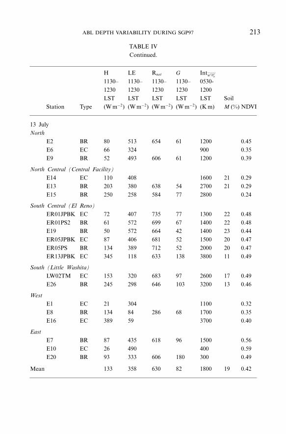
TABLE IV
Flux tower data for 12 and 13 July 1997: sensible heat flux (H ), latent heat flux (LE),net radiation (Rnet), soil heat flux (G), integrated buoyancy flux from 0530 to 1200 LST(Intw′θ ′
v), ESTAR soil moisture (soil M) and AVHRR NDVI (NDVI).
H LE Rnet G Intw′θ ′v
1130– 1130– 1130– 1130– 0530-1230 1230 1230 1230 1200LST LST LST LST LST Soil
Station Type (W m−2) (W m−2) (W m−2) (W m−2) (K m) M (%) NDVI
12 JulyNorth
E2 BR 127 474 659 58 1800 0.32E6 EC 72 353 800 31 0.44E9 BR 91 461 611 59 1300 29 0.24
North Central (Central Facility)
E14 EC 129 384 1800 28 0.15E13 BR 236 350 645 59 3000 28 0.15E15 BR 269 263 602 69 3000 0.45
South Central (El Reno)
ER01JPBK EC 104 386 742 73 1600 27 0.36ER01PS2 BR 89 547 702 66 1800 27 0.36E19 BR 92 536 669 41 1400 28 0.39ER05JPBK EC 123 391 685 55 1800 25 0.44ER05PS BR 166 355 715 55 2400 25 0.44ER13JPBK EC 278 121 643 140 3100 15 0.45
South (Little Washita)
LW02TM EC 157 306 690 78 2600 22 0.51E26 BR 248 305 651 98 3100 18 0.51
West
E1 EC 200 287 2100 0.43E8 BR 137 81 291 73 1700 0.26E16 EC 358 120 3200 0.44
East
E7 BR 52 377 496 67 900 0.54E10 EC 15 532 400 0.49E20 BR 85 344 604 175 100 0.52
Mean 151 349 627 78 1900 26 0.39
ABL DEPTH VARIABILITY DURING SGP97 213
TABLE IV
Continued.
H LE Rnet G Intw′θ ′v
1130– 1130– 1130– 1130– 0530-1230 1230 1230 1230 1200LST LST LST LST LST Soil
Station Type (W m−2) (W m−2) (W m−2) (W m−2) (K m) M (%) NDVI
13 JulyNorth
E2 BR 80 513 654 61 1200 0.45E6 EC 66 324 900 0.35E9 BR 52 493 606 61 1200 0.39
North Central (Central Facility)
E14 EC 110 408 1600 21 0.29E13 BR 203 380 638 54 2700 21 0.29E15 BR 250 258 584 77 2800 0.24
South Central (El Reno)
ER01JPBK EC 72 407 735 77 1300 22 0.48ER01PS2 BR 61 572 699 67 1400 22 0.48E19 BR 50 572 664 42 1400 23 0.44ER05JPBK EC 87 406 681 52 1500 20 0.47ER05PS BR 134 389 712 52 2000 20 0.47ER13JPBK EC 345 118 633 138 3800 11 0.49
South (Little Washita)
LW02TM EC 153 320 683 97 2600 17 0.49E26 BR 245 298 646 103 3200 13 0.46
West
E1 EC 21 304 1100 0.32E8 BR 134 84 286 68 1700 0.35E16 EC 389 59 3700 0.40
East
E7 BR 87 435 618 96 1500 0.56E10 EC 26 490 400 0.59E20 BR 93 333 606 180 300 0.49
Mean 133 358 630 82 1800 19 0.42

214 ANKUR R. DESAI ET AL.
Figure 3. Image of a portion of the LASE flight track showing LASE relative aerosol back-scatter and ABL depth (black line) over the 1130 LST tracks (a) 12 July and (b) 13 July.Smoothed LASE ABL depth from south to north (along the centre spine of the ESTARdomain) for late morning and midday legs on (c) 12 July and (d) 13 July.
central region was shallow and slow growing (<1000 m, <150 m h−1), whilethe ABL in the north central region grew faster to reach a depth ofapproximately 1400 m. The rapid ABL deepening (approximately 500 m h−1)in the north central region occurred earlier in the northern subsection(36.5–37◦ N) than the southern subsection (36–36.5◦ N).
Midday ABL depths on 13 July at 1130 LST were overall lower (mean1006 m ± 141 m) especially at the southern end (Figure 3). ABL depth inthe late morning was highest in the south (1000 m) and central (900 m),but by midday, ABL depths at the northern end matched the southern end

ABL DEPTH VARIABILITY DURING SGP97 215
(1200–1300 m). This shift in ABL depth pattern is also seen in balloonsoundings, but at a later time between the midday and afternoon soundings(Table II). Average sounding midday depth over the P-3 track was slightlylower (941 m) than LASE. Growth rates from 1015 to 1230 LST were high-est (200 m h−1) in the north, consistent with what was observed in the mid-day and afternoon soundings. In contrast to the soundings, very little ABLdeepening was observed along the southern end of the track, with someslow growth (approximately 150 m h−1) in the south central region. ABLdepths appear to even have declined by 200 m from 1045 LST to 1200 LSTnear 36.25◦ N, similar to what was observed by the central area sounding,which showed a 150 m decrease in ABL depth from midday to afternoon.
5.2. Observed surface energy fluxes
Spatial variation in time-integrated surface buoyancy flux (Table IV) aver-aged by region reflected the variation seen in ABL depth on 12 July(Table II). Mean time-integrated surface buoyancy flux in the south, south-central, north-central and north regions was 2850, 2010, 2600, 1300 K m,respectively, similar in pattern to mean midday region-average sensible heatflux. Latent heat fluxes were largest in the south-central and north regions.These patterns were remarkably similar to the variation in midday ABLdepth from south to north (high, low, moderately high, low). In contrast,a larger average time-integrated surface buoyancy flux was seen in the west(average, 2300 K m) compared to the east (average, 460 K m), opposite tothe pattern of the midday ABL depth, which was slightly higher in theeast (850 m east, 675 m west). It appears that the larger magnitude surfacebuoyancy flux in the west was unable to lead to a larger ABL depth therebecause the inversion strength was much higher in the west compared toall other sounding locations on 12 July (Table II),
Similar patterns in time-integrated surface buoyancy flux were observedon 13 July, though the total flux magnitude was slightly lower (TableIV). Region average time-integrated buoyancy flux was 2900, 1900, 2400,1100 K m for the south, south-central, north-central and north regions,respectively, which were on average 7% smaller than 12 July. Midday sensi-ble heat fluxes were smaller on 13 July, while latent heat fluxes were larger.Midday net radiation and soil heat flux were similar on both days. Thesevariations are reflected in the sounding observed ABL depth in midday, butby afternoon the ABL grew in the northern region and declined the cen-tral region. LASE observed ABL depths also showed greater values to thenorth, despite the low surface buoyancy fluxes there. This may have beendue to the larger variation in inversion strength from south to north on 13July (Table II).
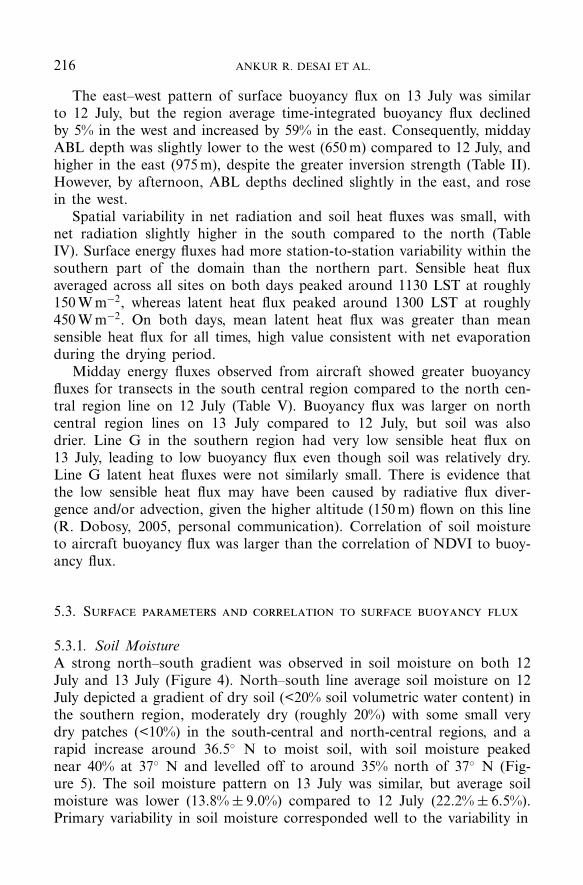
216 ANKUR R. DESAI ET AL.
The east–west pattern of surface buoyancy flux on 13 July was similarto 12 July, but the region average time-integrated buoyancy flux declinedby 5% in the west and increased by 59% in the east. Consequently, middayABL depth was slightly lower to the west (650 m) compared to 12 July, andhigher in the east (975 m), despite the greater inversion strength (Table II).However, by afternoon, ABL depths declined slightly in the east, and rosein the west.
Spatial variability in net radiation and soil heat fluxes was small, withnet radiation slightly higher in the south compared to the north (TableIV). Surface energy fluxes had more station-to-station variability within thesouthern part of the domain than the northern part. Sensible heat fluxaveraged across all sites on both days peaked around 1130 LST at roughly150 W m−2, whereas latent heat flux peaked around 1300 LST at roughly450 W m−2. On both days, mean latent heat flux was greater than meansensible heat flux for all times, high value consistent with net evaporationduring the drying period.
Midday energy fluxes observed from aircraft showed greater buoyancyfluxes for transects in the south central region compared to the north cen-tral region line on 12 July (Table V). Buoyancy flux was larger on northcentral region lines on 13 July compared to 12 July, but soil was alsodrier. Line G in the southern region had very low sensible heat flux on13 July, leading to low buoyancy flux even though soil was relatively dry.Line G latent heat fluxes were not similarly small. There is evidence thatthe low sensible heat flux may have been caused by radiative flux diver-gence and/or advection, given the higher altitude (150 m) flown on this line(R. Dobosy, 2005, personal communication). Correlation of soil moistureto aircraft buoyancy flux was larger than the correlation of NDVI to buoy-ancy flux.
5.3. Surface parameters and correlation to surface buoyancy flux
5.3.1. Soil MoistureA strong north–south gradient was observed in soil moisture on both 12July and 13 July (Figure 4). North–south line average soil moisture on 12July depicted a gradient of dry soil (<20% soil volumetric water content) inthe southern region, moderately dry (roughly 20%) with some small verydry patches (<10%) in the south-central and north-central regions, and arapid increase around 36.5◦ N to moist soil, with soil moisture peakednear 40% at 37◦ N and levelled off to around 35% north of 37◦ N (Fig-ure 5). The soil moisture pattern on 13 July was similar, but average soilmoisture was lower (13.8% ± 9.0%) compared to 12 July (22.2% ± 6.5%).Primary variability in soil moisture corresponded well to the variability in

ABL DEPTH VARIABILITY DURING SGP97 217
TA
BL
EV
Lon
gE
Zan
dTw
inO
tter
line-
aver
aged
fluxe
sfo
rfli
ght
legs
clos
est
to12
00L
ST,
EST
AR
line-
aver
aged
soil
moi
stur
ean
dA
VH
RR
ND
VI
for
12an
d13
July
1997
.
Tim
esH
LE
w′ θ
′ vA
vg.
soil
ND
VI
Dat
eL
ine
Pla
tfor
mL
atit
ude
Lon
gitu
de(L
ST)
(Wm
−2)
(Wm
−2)
(Km
s−1)
moi
stur
e(%
)
12Ju
lyN
orth
Cen
tral
(Cen
tral
Faci
lity)
DL
ong
EZ
36◦ 1
2′ 37"
97◦ 3
6′ 57"
1213
102
285
0.11
190.
26S
outh
Cen
tral
(El
Ren
o)
RL
ong
EZ
35◦ 3
3′ 24"
98◦ 0
5′ 20"
1040
143
236
0.14
140.
46R
Twin
Ott
er35
◦ 33′ 2
4"98
◦ 05′ 1
2"11
4318
335
50.
1814
0.46
ETw
inO
tter
35◦ 5
2′ 16"
97◦ 5
1′ 21"
1002
221
155
0.20
110.
2713
July
Nor
thC
entr
al(C
entr
alFa
cilit
y)
BTw
inO
tter
36◦ 1
1′ 06"
97◦ 3
7′ 51"
1133
208
339
0.20
110.
29D
Twin
Ott
er36
◦ 12′ 3
6"97
◦ 36′ 4
5"12
0619
428
20.
1911
0.31
Sou
th(L
ittl
eW
ashi
ta)
GL
ong
EZ
34◦ 5
0′ 24"
97◦ 5
9′ 51"
1220
4527
40.
0616
0.49

218 ANKUR R. DESAI ET AL.
Figure 4. ESTAR derived surface soil moisture (volumetric percentage) on (a) 12 July and(b) 13 July.
35 36 37 38
Latitude (degrees N)
0
10
20
30
40
50
% s
oil m
oist
ure
34.5 35 35.5 36 36.5 37
Latitude (degrees N)
0
10
20
30
40
50
% s
oil m
oist
ure
(a) (b)
12 July 13 July
Figure 5. Mean ESTAR derived surface soil moisture from south to north averaged acrossall pixels from east to west for (a) 12 July and (b) 13 July. One standard deviation is shownin grey.
antecedent precipitation (Figure 2), however the secondary southern max-imum (between 34.75 and 35.5◦ N) in soil moisture was not reflected inthe precipitation gradient. The soil on average was drier on 13 July (mean13.8% ± 9.0%) than 12 July (mean 22.2% ± 6.5%), consistent with the dry-ing that occurred after the precipitation. No strong east–west patterns insoil moisture were observed, but observations were limited by the relativelynarrow field of view for ESTAR.

ABL DEPTH VARIABILITY DURING SGP97 219
Figure 6. NOAA AVHRR NDVI for late afternoon of 12 and 13 July. An outline of theESTAR domain is included for reference. Letters refer to regions of interest: N = northernarea, CF = Central Facility area, ER = El Reno (south-central) area, LW = Little Washita(south) area.
5.3.2. NDVINDVI values revealed a large-scale pattern of increasing vegetation covergoing from west to east, but no strong north–south variation (Figure 6).There were two basic regions, a western (98.5–100◦ W) and central (97–98.5◦ W) region of NDVI 0.3–0.4 and an eastern region (95–97◦ W)with NDVI 0.5–0.6, with a sharp change from 96.5 to 97.5◦ W longitude(Figure 7). Region-averaged NDVI was related to the region-averaged sur-face buoyancy and sensible heat fluxes, which were larger in the westernand central regions compared to the eastern region, and vice versa forlatent heat flux.
Unlike soil moisture or surface energy fluxes, vegetation greenness didnot have any strong north–south gradients along the central part of thedomain (Figure 7). NDVI was lowest (0.25–0.35) in the north centralregion, highest in the south central region (0.4–0.5) and moderate in thesouth (0.4) and the north (0.35–0.4). The gradient was the same on 12 and13 July. These gradients were not strongly related to patterns of surfaceenergy flux or ABL depth.
There was very little difference between mean NDVI on 12 July (0.42 ±0.11) and 13 July (0.43 ± 0.12), which is not surprising. The slight increasein mean NDVI on 13 July occurred primarily due to an approximately 0.05increase in NDVI among the higher NDVI pixels, whereas the areas withlow NDVI remained the same. Direct comparison of ESTAR soil moisturepixels to NDVI showed no correlation.

220 ANKUR R. DESAI ET AL.
35 36 37 38 39
Latitude (degrees N)
0.1
0.2
0.3
0.4
0.5
0.6
0.7
ND
VI
100 99 98 97 96Longitude (degrees W)
0.1
0.2
0.3
0.4
0.5
0.6
0.7
ND
VI
35 36 37 38 39
Latitude (degrees N)
0.1
0.2
0.3
0.4
0.5
0.6
0.7
ND
VI
99 98 97 96Longitude (degrees W)
0.1
0.2
0.3
0.4
0.5
0.6
0.7
ND
VI
34 34
95 95100
(a) (b)
(d)(c)
12 July
12 July 13 July
13 July
Figure 7. Mean NDVI from south to north averaged across 96.5◦ W to 98.5◦ W for (a) 12July and (b) 13 July and mean NDVI from west to east averaged across 36◦ N to 37◦ N for(c) 12 July and (d) 13 July. One standard deviation is shown in grey.
5.3.3. Relationship of Surface Parameters to Surface Buoyancy FluxNo strong correlation was found between daytime NDVI and observedtotal integrated surface buoyancy flux from all surface stations in theSGP97 domain from 0530 to 1200 LST on 12 July (r2 = 0.02) or 13 July(r2 = 0.05) (Figure 8). Correlations between NDVI and sensible heat flux,latent heat flux, Bowen ratio and evaporative fraction were similarly weak(not shown). In contrast, there was a strong correlation between soil mois-ture and time-integrated observed surface buoyancy flux from 0530 to 1200LST for 12 and 13 July (Figure 9). This correlation was stronger on 13 July

ABL DEPTH VARIABILITY DURING SGP97 221
F = –1.0 ± 13.0 * NDVI + 2.3 ± 6.9
r2 = 0.02χ sq. probability = 0.00
12 July, 1230 LST(a) (b)
NDVI
For
cing
(K
m *
10
3)
0.0 0.2 0.4 0.6 0.80
2
4
6
8
10
F = –3.9 ± 16.0 * NDVI + 3.5 ± 2.1
r2 = 0.05
13 July, 1230 LST
χ sq. probability = 0.00
For
cing
(K
m *
10
3)
NDVI
0.0 0.2 0.4 0.6 0.80
2
4
6
8
10
RMSE = 0.81 MARE = 51% RMSE = 0.97 MARE = 72%
Figure 8. Correlation of NDVI to integrated buoyancy flux from 0530 to 1200 LST on (a)12 July and (b) 13 July. Horizontal error bars represent 3×3 pixel misalignment error whilevertical error bars represent a typical 10% error in turbulent flux measurements.
(r2 = 0.80) than 12 July (r2 = 0.66). These correlations were stronger thanregressions between soil moisture and mean or midday sensible heat flux,latent heat flux, Bowen ratio or evaporative fraction (not shown). Meanabsolute relative error (MARE) was on average 15%, similar in range tothe sum of estimated errors for soil moisture and surface fluxes. Fit slopewas steeper on 13 July than 12 July, reflecting the smaller variability ofsoil moisture across flux towers. The difference in the slopes, however, wassmaller than the uncertainty in them. Fit intercepts were similar on bothdays. The similarity of soil moisture to patterns of surface fluxes and ABLdepth suggests that soil moisture was a major determinant of both, espe-cially on 12 July.
Applying the linear regression and the sinusoidal model described inEquation (3), we can simulate with high correlation (r2 = 0.78) and smallRMSE (0.04 K m s−1 ≡ 50 W m−2) tower-observed half-hourly surface buoy-ancy fluxes between 0530 and 1230 LST (Figure 10a). The model alsoreproduced the variations in daytime (0900–1230 LST) airplane line-averageflux with high correlation (r2 =0.73), but it overestimated daytime airplaneline-average buoyancy flux by an average of 0.08 K m s−1 (100 W m−2) (Fig-ure 10b). This overestimation was larger than the uncertainties in eithermodel or airplane flux.
5.4. Modelled ABL depth
The strong correlation between surface soil moisture and time-integratedsurface buoyancy flux along with the 1-D ABL model were used to model

222 ANKUR R. DESAI ET AL.
r2 = 0.64
F = –0.18 ± 0.07 * SM + 6.80 ± 2.02
χ sq. probability = 0.95
12 July, 1230 LST(a) (b)
Soil Moisture (%)
For
cing
(K
m *
103 )
0 10 20 30 40 500
2
4
6
8
10
r2 = 0.80
F = –0.24 ± 0.10 * SM + 6.65 ± 2.52
13 July, 1230 LST
χ sq. probability = 0.99
For
cing
(K
m *
103 )
Soil Moisture (%)
0 10 20 30 40 500
2
4
6
8
10
RMSE = 0.51, MARE=16% RMSE = 0.41, MARE=14%
Figure 9. Correlation of ESTAR derived soil moisture to total integrated buoyancy fluxfrom 0530 to 1200 LST on (a) 12 July and (b) 13 July. Horizontal error bars represent instru-ment validation error and a 3×3 pixel misalignment error while vertical error bars representa typical 10% error in turbulent flux measurements. Dotted lines denote maximum observedtime-integrated net radiative forcing and minimum observed integrated buoyancy flux, whichlimit the regression model extrapolated buoyancy fluxes for drier or moister than observedsoil moisture.
0 0.1 0.2 0.30
0.1
0.2
0.3
0 0.1 0.2 0.30
0.1
0.2
0.3
r2 = 0.73RMSE = 0.09
Aircraft leg average w’θv’ (K m s-1)
Mod
eled
w’θ
v’ (K
m s
-1)
Mod
eled
w’θ
v’ (K
m s
-1)
Flux tower w’θv’ (K m s-1)
r2 = 0.78RMSE = 0.04
(a) (b)
Mean error = 0.0004 Mean error =0.08
Figure 10. Relationship of modelled surface buoyancy flux to (a) half-hourly tower-observedsurface buoyancy flux, and (b) leg averaged aircraft buoyancy flux on 12 and 13 July from0530 to 1230 LST.

ABL DEPTH VARIABILITY DURING SGP97 223
12 July 13 July
Tim
e (L
ST
)
Tim
e (L
ST
)
Latitude (degrees N) Latitude (degrees N)
35 36 37 38 35 35.5 36 36.5 3734.5
9
10
11
1
9
10
11
12
600
800
800
1000
1200
1200
14001600
1600
600
600
800
1000
1200
140016
00
1000
(a) (b)
Figure 11. Modelled ABL depth (100 m contours) as a function of latitude and time for (a)12 July and (b) 13 July.
ABL depth along the P-3 track. Model results showed ABL depth vari-ability increasing with time as differential surface forcing allowed the ABLdepth to increase faster in regions with low soil moisture compared toregions with high soil moisture (Figure 11). Spatial variations in ABLdepth driven by spatial variability in both surface forcing and morninginversion strength were smoothed and shifted north by advection.
On 12 July, ABL growth was initially fastest in the north-central regionwhile southern region depths steadily rose but quickened in growth rateafter 1100 LST, in contrast to LASE observations that showed ABLgrowth occurring earlier in the south and later in the north central region.Consequently, the model overpredicted ABL growth in the north-centralregion based on central sounding results, but was better able to predictheights in regions near the northern and southern soundings (Table II).South-central ABL depth grew at the same rate as the southern region inthe early morning, but then slowed down after 0930 LST. The ABL inthe north had the slowest growth. By midday on 12 July, highest depthswere seen in the southern and north-central regions, lowest depths in thenorth, and moderate depths in the south-central region, in good agreement(r2 = 0.45 for 1130 LST) with LASE observations (Figure 12). By 1215LST, modelled ABL depth variations were shifted too far north by approx-imately 0.5 degrees latitude, which translates to 60 km. Despite accuratelyreproducing variations in amplitude of ABL depth across the P-3 track,the north-central and south-central region depths were overestimated, whilesouthern and northern region depths were well matched though underes-timated at the far southern end, with an average RMSE of 375 m. Mean

224 ANKUR R. DESAI ET AL.z i (
m)
Latitude (degrees N)
z i (m
)
1130 LST 12 July
35 36 37 38500
1000
1500
2000
2500
500 2500500
2500r2 = 0.45RMSE = 362
Latitude (degrees N)
1045 LST 13 July
35 35.5 36 36.5 37
500
1000
1500
2000
2500
34.5
500 2500500
2500r2 = 0.60RMSE = 129
Latitude (degrees N)z i (
m)
1215 LST 12 July
35 36 37 38500
1000
1500
2000
2500
500 2500500
2500r2 = 0.52RMSE = 375
r2 = 0.04RMSE = 210
Latitude (degrees N)
z i (m
)
1130 LST 13 July
35 35.5 36 36.5 37
500
1000
1500
2000
2500
34.5
500 2500500
2500
r2=0.54
(a)
(c) (d)
(b)
Figure 12. Comparison of LASE observed ABL depth (dotted line) to modelled ABL depthwith variable surface forcing (black line) and to modelled ABL depth with constant surfaceforcing (dashed line) on 12 July at (a) 1130 LST and (b) 1215 LST, and on 13 July at (c)1045 LST and (d) 1130 LST. Also shown are scatter plots of relationship of observed (x-axis) to modelled (y-axis) ABL depth with variable forcing.
model ABL depth across the whole track was 140 m larger than observedfor both the 1130 and 1215 LST tracks. Midday LASE-observed ABLdepth gradient from south to north (−2.2 m km−1) was well predicted bythe model (−2.4 m km−1).
On 13 July, modelled ABL had a steadily declining ABL growth ratefrom south to north (Figure 11), in contrast to LASE observations, whichshowed little late morning growth in the southern region and fastest growthin the late morning for the northern region. Growth rates in the north-central and south-central region were similar to LASE. After midday, the

ABL DEPTH VARIABILITY DURING SGP97 225
south-central region modelled ABL had rapid growth, similar to observa-tions at the southern sounding (Table II). Midday sounding ABL depthswere well reproduced by the model. Outside of the northern region, corre-lations to late morning and midday LASE ABL depth were higher on 13July than 12 July (Figure 12). Mean ABL model depth was slightly higherin the model than observed by approximately 50 m and an RMSE of 170 maveraged across both tracks. On both tracks, the modelled ABL depth gra-dient from south to north was matched well for the late morning track(−2.3 m km−1 for model, −2.0 m km−1 for observed) but overestimated formidday (−2.1 m km−1 for model, −1.3 m km−1 for observed) outside of thenorthern end.
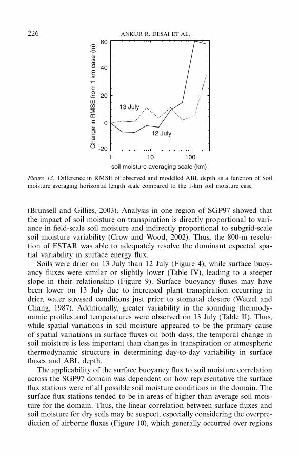
On both days, the use of ESTAR soil moisture to describe the variationin surface forcing led to a significantly improved prediction of LASE ABLdepth compared to the use of constant average surface forcing along thewhole track (dashed line, Figure 12). The constant forcing model underes-timated mean ABL depth, and ABL depth variations were dampened. Theprimary exception was the northern end of the midday 1130 LST trackon 13 July, where the constant forcing based model reproduced the LASEobserved gradient (7.1 m km−1), while the ESTAR based model had theopposite gradient (−1.0 m km−1). When comparing the RMSE of observedto modelled ABL depth using coarse resolution soil moisture compared tothe high resolution soil moisture case, a large jump in RMSE occurred at64 km for 12 July and 128 km for 13 July (Figure 13), suggesting that ABLdepth was primarily sensitive to soil moisture scales smaller than these val-ues. Modelled ABL depth performed poorly at reproducing observed spa-tial gradient in LASE-observed ABL depth at small horizontal averagingscales and better at larger averaging scales on both days, with little changein performance above 100 km.
6. Discussion
6.1. Effect of soil moisture on surface forcing
The significant correlation between surface buoyancy flux and remotelysensed soil moisture suggests that 1-km scale average soil moisture affectedsurface energy fluxes measured from short towers with footprints rangingfrom 100s to 1000s of metres. The general gradient of wet soils to the northand more variable but dryer soils to the south, with very dry soils in thesouthern end and north-central region, correlated closely to the observedvariability in surface buoyancy flux. Wavelet analysis revealed that SGP97remotely sensed surface energy flux variability was dominated by varia-tions at the 400–800 m scale, coincident with average agricultural field size
226 ANKUR R. DESAI ET AL.
1 10 100-20
0
20
40
60
13 July
12 July
soil moisture averaging scale (km)
Cha
nge
in R
MS
E fr
om 1
km
cas
e (m
)
Figure 13. Difference in RMSE of observed and modelled ABL depth as a function of Soilmoisture averaging horizontal length scale compared to the 1-km soil moisture case.
(Brunsell and Gillies, 2003). Analysis in one region of SGP97 showed thatthe impact of soil moisture on transpiration is directly proportional to vari-ance in field-scale soil moisture and indirectly proportional to subgrid-scalesoil moisture variability (Crow and Wood, 2002). Thus, the 800-m resolu-tion of ESTAR was able to adequately resolve the dominant expected spa-tial variability in surface energy flux.
Soils were drier on 13 July than 12 July (Figure 4), while surface buoy-ancy fluxes were similar or slightly lower (Table IV), leading to a steeperslope in their relationship (Figure 9). Surface buoyancy fluxes may havebeen lower on 13 July due to increased plant transpiration occurring indrier, water stressed conditions just prior to stomatal closure (Wetzel andChang, 1987). Additionally, greater variability in the sounding thermody-namic profiles and temperatures were observed on 13 July (Table II). Thus,while spatial variations in soil moisture appeared to be the primary causeof spatial variations in surface fluxes on both days, the temporal change insoil moisture is less important than changes in transpiration or atmosphericthermodynamic structure in determining day-to-day variability in surfacefluxes and ABL depth.
The applicability of the surface buoyancy flux to soil moisture correlationacross the SGP97 domain was dependent on how representative the surfaceflux stations were of all possible soil moisture conditions in the domain. Thesurface flux stations tended to be in areas of higher than average soil mois-ture for the domain. Thus, the linear correlation between surface fluxes andsoil moisture for dry soils may be suspect, especially considering the overpre-diction of airborne fluxes (Figure 10), which generally occurred over regions
ABL DEPTH VARIABILITY DURING SGP97 227
with lower line-average soil moisture than for the surface flux towers. Fortu-nately, most of the domain did not have very dry soil.
The sparse and low vegetation in the study area means that surfaceevaporation generally dominates over plant transpiration. Thus, given thesparse vegetation and 10 July rainstorm, it was not surprising that surfacesoil moisture availability was the main determinant of surface buoyancyfluxes on these two clear, sunny days. Bindlish et al. (2001) also showedhigh correlation between ESTAR soil moisture and modelled surface sen-sible heat fluxes from late June to mid July, but the correlation declinedwith increasing NDVI, especially for NDVI above 0.4. Thus, we suspectthat the relationship between soil moisture and surface energy flux in themore heavily vegetated eastern region may not have been as strong.
Unlike soil moisture, the north–south pattern in NDVI did not correlateto the pattern of surface energy fluxes (Figure 8) or ABL depth, contraryto some observations in the region made over short distances by aircraftthat showed stronger relationship between vegetation cover and surfaceenergy flux (Chen et al., 2003; J. Sun, 2002, personal communication).Even though the large-scale west–east increase in NDVI was reflected inthe gradient of declining surface buoyancy flux from west to east, point-by-point correlation was poor. NDVI spatial variability may have been toosmall to capture energy flux variability in an area with the homogeneousvegetation found in our study area. NDVI values tend to remain constantover longer time periods, corresponding to the evolution of the growingseasons and the agricultural cultivation of winter wheat. Thus, the longerterm evolution of surface energy fluxes (i.e. due to changes in plant transpi-ration and ground cover) would be constrained by vegetation cover change,while rapid greening in the early part of the growing season can signifi-cantly affect the short-term evolution of surface energy fluxes (Chen et al.,2003). However, these effects were not important on the two days in ourcase study.
Our goal was not to construct a new method to remotely sense sur-face energy fluxes, but rather to determine what surface parameter (soilmoisture or vegetation greenness) had the most influence on surface energyfluxes in our case study, and then to use that information to model theinfluence of the surface parameter on ABL depth. Many researchers haveattempted to create and test methodologies for the measurement or cal-culation of surface fluxes through satellite remote sensing devices (e.g.,Brutsaert et al., 1993; Pelgrum and Bastiaanssen, 1996; Chehbouni et al.,1997; Doran et al., 1998; Gao et al., 1998; Rabin et al., 2000; Ridder,2000; Roerink and Menenti., 2000; Song and Wesely, 2003; Diak et al.,2004). These methods can be either universal (i.e. a relationship for alllandscape types) or landscape-dependent (e.g. works only for grasslands),and statistically (e.g. linear correlation) or physically based (i.e. modelled

228 ANKUR R. DESAI ET AL.
from first principles). For example, the Atmospheric Land Exchange Inver-sion (ALEXI) coupled soil and vegetation model (Anderson et al., 1997),which relies on remote sensing of surface temperature over multiple timesin the day, sounding-derived morning thermodynamic structure and spatialinformation on soil and vegetation cover, has been used with some successin the Southern Great Plains region (e.g., Kustas et al., 1999; Mecikalskiet al., 1999; French et al., 2000). Our results suggest that, in cases of sig-nificant antecedent precipitation spatial variability, remotely sensed surfacesoil moisture has a valuable role in improving model prediction or remotelysensed observations of surface energy fluxes and, in turn, estimating meso-scale ABL depth variability.
6.2. Effect of surface forcing on ABL depth
6.2.1. Role of Initial Thermodynamic StructureComparison of modelled ABL depths (Figure 11) to sounding and LASEobserved ABL depths, with and without spatially variability forcing (Figure12), suggests that soil moisture variability was the main determinant of ABLdepth variability, especially on 12 July. Variability in ABL depth occurredeven though all initial early morning profiles on 12 July had roughly similarincreases in temperature with height in the first 1000 m, while greater var-iability in inversion strength was observed on 13 July (Table II). Inversionstrength variability appeared to have been more important in the easternand western regions, where strong surface forcing in the western region didnot produce a large ABL depth due to a strong inversion strength, whileweak surface forcing in the eastern region was able to erode a relativelyweaker inversion. Inversion strength was significantly greater (from 7% to80% larger) on 13 July than 12 July (Table II), and was a major reason that,despite drier soil moisture, the ABL depth was lower on 13 July, in additionto the larger subsidence and slightly lower surface buoyancy fluxes.
Variability in the choice of initial sounding caused average variations of250 m across the LASE midday track, with a range of 475 m in the south-ern end and 130 m in the northern end, averaged over both days (Figure14a and b). Additionally, given an arbitrary amount of forcing to any onesounding, a gradient of higher to lower potential ABL depth was observedfrom south to north (Figure 14c and d). These variations were smallerthan the primary variations in ABL depth on 12 July, but similar to thevariations on 13 July. Therefore, while surface forcing variability was theprimary cause of ABL depth variability, the variation in atmospheric ther-modynamic structure was of secondary importance on 12 July and of near-equal importance on 13 July.

ABL DEPTH VARIABILITY DURING SGP97 229
Latitude (degrees N)
zi (
m)
Latitude (degrees N)z i (
m)
1130 LST 12 July
35 36 37 38500
1000
1500
2000
2500
35 35.5 36 36.5 37500
1000
1500
2000
2500
34.5
1130 LST 13 July
C1
C1
B1
B1
B6
B6
0 2 4 6 8 10 12 14Forcing (MJ m-2)
0
500
1000
1500
2000
2500
zi (
m)
0 2 4 6 8 10 12 14Forcing (MJ m-2)
0
500
1000
1500
2000
2500
zi (
m)
C1
B1
B6
C1
B1
B6
12 July 13 July
(a) (b)
(d)(c)
Figure 14. Effect of initial sounding choice (B1 = north, C1 = central, B6 = south) on mod-elled ABL depth for (a) 12 July and (b) 13 July (dotted line is observed) and potential attain-able ABL depth for arbitrary amounts of total forcing for different initial early morningsoundings on (c) 12 July and (d) 13 July.
The results also confirm that the initial thermodynamic structure isimportant in determining locations of rapid ABL growth (Findell andElfatir, 2003). The ABL initially grows steadily as surface buoyancy andthe entrainment of dry air erodes the morning inversion (Deardorff, 1980).If forcing is strong enough (due, for example, to dry soil) to realizethe convective triggering potential (CTP) (Findell and Elfatir, 2003), thencontinued forcing leads to rapid ABL growth. The transition to rapidgrowth occurred in the southern part of our study area, but not in thenorthern part on 12 July. On 13 July, rapid growth was evident in boththe southern and northern soundings, but not until later in the day. Given

230 ANKUR R. DESAI ET AL.
Latitude (degrees N)
zi (
m)
Latitude (degrees N)
zi (
m)
1130 LST 12 July 1130 LST 13 July
35 36 37 38500
1000
1500
2000
2500
35 35.5 36 36.5 37500
1000
1500
2000
2500
34.5
Latitude (degrees N)
dzi (
m)
Latitude (degrees N)
dzi (
m)
1130 LST 12 July 1130 LST 13 July
35 36 37 38-600
-300
0
300
600
35 35.5 36 36.5 37-600
-300
0
300
600
34.5
Advection Advection
Convergence/Divergence
SubsidenceSubsidence
Convergence/Divergence
(a)
(c) (d)
(b)
Figure 15. Modelled ABL depth with no winds (black line) and constant wind (dashed line)for (a) 12 July and (b) 13 July, and net time-integrated effect of advection (black line), con-vergence/divergence (grey line) and subsidence (straight line) on modelled ABL depth for (c)12 July and (d) 13 July.
the underprediction of ABL depth by the model in the far southern endof the domain on 12 July, it may be the case that the CTP in that regionwas lower than the southern sounding CTP, or alternatively the entrain-ment flux was underestimated.
6.2.2. Role of Advection, Convergence/Divergence, and SubsidenceAdvection, convergence/divergence and subsidence all had the impact ofimproving the relationship of model to observed ABL depth (Figure 15).When the model was run without these three effects, modelled ABL depth

ABL DEPTH VARIABILITY DURING SGP97 231
(Figure 15a and b, solid line) was poorly correlated to observed ABLdepth, with little relation between the variations in soil moisture and ABLdepth except at the largest of scales (>200 km). When the model wasrun with variable forcing and large-scale subsidence, but a constant windspeed (Figure 15a and b, dashed line), an improvement between modeland observed ABL depth was found. For 12 July, however, the constantwind speed model had poorer performance at reproducing the amplitude,location and wavelength of the observed secondary south-central minimumand north-central maximum in ABL depth than the variable wind speedmodel (Figure 12), suggesting that convergence/divergence of winds workedin tandem with soil moisture variations to generate ABL depth variation.In contrast, on 13 July, the constant wind speed model was better ableto capture the decrease in ABL depth at 36.25◦ N than the variable windspeed model. Since our observations were limited to five soundings withno model dynamics, errors in sounding wind speeds and interpolation mayhave led to an incorrect convergence/divergence term on 13 July, which canbe better captured with a 3-D mesoscale model.
Integrating each right-hand side term of Equation (5) with respect totime shows the net effect of these terms upon midday ABL depth (Fig-ure 15c and d). Additionally, the advection term was split into an advectiveand convergence/divergence component:
∫ t1
t0
∂uzi
∂x=
∫ t1
t0
u∂zi
∂x+
∫ t1
t0
zi
∂u
∂x. (7)
The net effect of advection was to shift northward and to smooth thesurface forcing. Subsidence reduced ABL depths by 100 m on 12 Julyand 290 m on 13 July as atmospheric pressure increased in the region.Model ABL depths on 13 July would be significantly overestimated withoutthe subsidence term. Convergence/divergence due to changes in northwardalong-track wind speed on 12 July led to amplification of the secondaryminimum and maximum of ABL depth that was initially set-up by theadvection of variable surface forcing. With constant forcing, a secondaryminimum and maximum pattern exists but the amplitude, wavelength andwidth are all too small (Figure 12a, dashed line). The same is true for thecase of constant wind speed (Figure 15a, dashed line).
Segal and Arritt (1992) show from theoretical arguments that 50–100 km mesoscale circulations or inland breezes can occur from contrastsin surface forcing arising from soil moisture gradients. Their scaling anal-ysis suggests that, given the wind speeds and mean forcing observed inour case study, 50-km horizontal scale variations in forcing can generatesuch circulations. Our scaling results showed that ABL depth respondedto 50–100 km scale variations in surface forcing (Figure 13), suggesting the

232 ANKUR R. DESAI ET AL.
possibility of secondary circulations. In Part II of our study, 3-D modelsimulations show that an inland breeze can be generated by the soil mois-ture gradient (Reen et al., submitted). The lack of a secondary maxi-mum/minimum structure on 13 July may have been due to the increasedlarge-scale subsidence, which has been shown in model studies to dampensurface forcing heterogeneity-induced circulations (Weaver, 2004). The lackof high-spatial density observations limits our ability to conclusively testthese assertions with our simple 1-D model.
6.2.3. Scales of ABL Depth and Surface ForcingOur results showed that variations in soil moisture on scales less than64 km on 12 July and less than 128 km on 13 July were able to explainvariations in ABL depth primarily for scales >100 km (Figure 13). Therewas poor correlation of modelled to observed ABL depth variation atsmall scales (<50 km), reflecting both model deficiencies and the effect ofconvective mixing and advection of surface heterogeneity in the ABL, ashas been observed in large-eddy simulation studies (Avissar and Schmidt,1998). Smaller scale observed variability in ABL depth was most likely afunction of turbulent fluctuations.
Mahrt (2000) shows that the relationship between spatial variability insurface properties to spatial variability in ABL structure is expected tobe directly proportional to the scale of surface heterogeneity and inverselyproportional to wind speed, atmospheric stability and mean ABL depth.From blending height arguments, Raupach and Finnigan (1995) argue thatthe minimum length scale of surface heterogeneity that can influence athermally-driven convective boundary layer is
Lmin = CUzi
w∗, (8)
where C is a constant shown to be 0.8 (Mahrt, 2000), U is the ABL windspeed, zi is ABL depth, and w∗ is the convective velocity scale:
w∗ =(
g
θv
zi
(w′θ ′
v
)s
)1/3
. (9)
An alternative scaling was derived by Wood and Mason (1991) for unstableconditions where surface heating is important:
Lwm =Cwmzi
Uθv(w′θ ′
v
)s
, (10)
where Cwm is a constant shown to be 3.1 × 10⁻³ (Mahrt, 2000). Mah-rt (2000) also notes that the largest scale of surface heterogeneity that

ABL DEPTH VARIABILITY DURING SGP97 233
could significantly affect variability in ABL depth is a function of the windspeed:
Lmax =TeU (11)
where Te is the entrainment time scale (Raupach and Finnigan, 1995), cor-responding to the length of time available for boundary-layer growth.
These lengths scales average to 4.5 km for Lmin, 63 km for Lwm and119 km for Lmax on 12 July and 4.0 km for Lmin, 46 km for Lwm and 127 kmfor Lmax on 13 July. Compared to our results, Lmin appears to be too small.Lmin and Lwm decreased on 13 July, but our results suggest that the lengthscale actually increased. It appears that, while the scale of surface hetero-geneity increased on 13 July, and therefore we might have expected a stron-ger influence of soil moisture on ABL depth, the absolute magnitude ofthe spatial variation in soil moisture decreased and early morning stabilityincreased in strength and spatial variation, leading to a decreased influenceof soil moisture on ABL depth at scales smaller than 100 km, larger thanboth Lmin and Lwm. It may also be possible that our simple 1-D model wasunable to model surface heterogeneity induced variations in ABL structureat smaller scales, which a more sophisticated 3-D mesoscale model couldcapture.
6.2.4. Mesoscale ModellingThe simple 1-D model used here is unable to include the effects of 3-Dadvection, wind field dynamic evolution and dynamic land-surface varia-tion on ABL depth. The model also suffers from a low data density forwind velocity. Part II explores methods for assimilating ESTAR high reso-lution soil moisture into the Penn State/NCAR MM5 mesoscale model forthe 12 July case (Reen et al., submitted). Since a mesoscale model is ableto simulate the 3-D atmospheric dynamics including convergence/diver-gence, mesoscale circulations, advection, entrainment, and is able to assim-ilate large area atmospheric and land surface boundary conditions andmodel dynamic changes in land-surface properties, it is expected that (1)the mesoscale model is better able to predict ABL structure than the 1-Dmodel used here, and (2) the assimilation of high-resolution soil moistureshould improve the predictions of ABL depth compared to coarser resolu-tion observations and models. Reen et al. (submitted) demonstrate both ofthese effects and illustrate the reasons for some of the shortcomings exhib-ited by the 1-D model.
234 ANKUR R. DESAI ET AL.
7. Conclusions
We examined land-surface forcing of ABL variability. Variations in surfacebuoyancy flux explained the general (>100 km) but not fine-scale mesoscalevariations in ABL depth in our case study. Remotely sensed soil moistureand vegetation cover were compared at points of known surface buoyancyflux. Soil moisture was shown to be the best predictor of surface buoyancyflux variability in these two case study days following precipitation. Thiscorrelation was significantly better than the correlation between vegetationgreenness and total forcing, suggesting that short term surface energy fluxvariability in the Southern Great Plains was driven more by soil moistureevaporation than vegetation cover. Although this result has been modelledand observed on the small scale before, the SGP97 study was a uniqueopportunity to observe this phenomenon on a larger scale, using a densenetwork of instruments along with high-resolution airborne ABL measure-ments.
The primary pattern of ABL development on 12 July was one of greaterABL depths in the southern end of the domain and a markedly differentregime of lower ABL depths in the northern end, with a secondary min-imum and maximum across the central part. The large-scale gradient wassuppressed on 13 July due to changes in initial atmospheric thermodynamicconditions with space and time, an increase in subsidence, and a decline inaverage surface forcing. The observed north-south gradient in ABL depthmatched well to the general north–south pattern of soil moisture and sur-face energy fluxes, but advection, convergence/divergence, subsidence andentrainment also were important determinants of ABL depth. The second-ary maximum and minimum in ABL depth on 12 July appear to have beencaused by variations in both wind velocity and soil moisture. The meso-scale model used in Part II provides more insight into the finer scale ABLstructure and the influence of variable surface forcing upon it.
One of the goals of the Southern Great Plains 1997 study was to val-idate soil moisture retrieval algorithms of ESTAR for the possible futureuse of passive microwave remote sensing in space. While the spatial reso-lution (10–30 km) of a space-borne passive microwave instrument would becoarser than was available for this study (Jackson et al., 1999), it would stillbe useful for characterizing mesoscale surface flux and ABL depth variabil-ity. Our study showed that variations in ABL depth due to surface energyflux on fair weather days with moderate wind speeds existed on scales of100 km, with a mesoscale model study suggesting even finer resolutions, atleast for our case study. The simple model described in this paper indi-cates that it is possible to examine the ABL depth using remotely-sensedsoil moisture and limited ground-based data at certain times and locations,

ABL DEPTH VARIABILITY DURING SGP97 235
and suggests that soil moisture is an important variable to include in mod-els of ABL development.
Acknowledgements
The authors wish to acknowledge Ronald Dobosy at NOAA Atmo-spheric Turbulence and Diffusion Division, J. Ian MacPherson of theNational Research Council Canada, Institute for Aerospace Research,Peggy LeMone of the National Center for Atmospheric Research andan anonymous reviewer for assistance with this manuscript. The authorsalso wish to thank Bill Kustas, John Preuger, Tilden Meyers and PatrickStarks for use of their flux data, the Atmospheric Radiation Measurement(ARM) Program sponsored by the U.S. Department of Energy, Office ofScience, Office of Biological and Environmental Research, Climate ChangeResearch Division, and all scientists and technical staff involved in collect-ing data during the field campaign. This work was funded in part by grantsfrom the U.S. National Aeronautics and Space Administration (NASA)Land Surface Hydrology Program, grant number NASA/NAG-1-193 andby the U.S. National Science Foundation (NSF), Directorate for Geoscienc-es, Division of Atmospheric Sciences, grant number ATM-0130349.
References
Anderson, J. C., Norman, J. M., Diak, G. R., Kustas, W. P., and Mecikalski, J. R.: 1997, ‘ATwo-source Time Integrated Model for Estimating Surface Fluxes using Thermal InfraredRemote Sensing’, Remote Sens. Environ. 60, 195–216.
Avery, T. E. and Berlin, G. L.: 1992, Fundamentals of Remote Sensing and Airphoto Interpre-tation, 5th ed., Prentice-Hall, Upper Saddle River, NJ, USA, 472 pp.
Avissar, R. and Pielke, R. A.: 1989, ‘A Parameterization of Heterogeneous Land-surface forAtmospheric Numerical Models and its Impact on Regional Meteorology’, Mon. Wea.Rev. 117, 2113–2136.
Avissar, R. and Schmidt, T.: 1998, ‘An Evaluation of the Scale at which Ground-SurfaceHeat Flux Patchiness Affects the Convective Boundary Layer using Large-Eddy Simula-tions’, J. Atmos. Sci. 55, 2666–2689.
Batchvarova, E. and Gryning, S.-E.: 1991, ‘Applied Model for the Growth of the DaytimeMixed Layer’, Boundary-Layer Meteorol. 65, 261–274.
Betts, A. K.: 2004, ‘Understanding Hydrometeorology using Global Models’, Bull. Am.Meteorol. Soc. 85, 1673–1688.
Betts, A. K. and Ball, J. H.: 1996, ‘The Land Surface–atmosphere Interaction: A Reviewbased on Observations and Global Modelling Perspectives’, J. Geophys. Res. 101(D3),7209–7225.
Bindlish, R., Kustas, W. P., French, A. N., Diak, G. R., and Mecikalski, J. R.: 2001, ‘Influ-ence of Near-surface Soil Moisture on Regional Scale Heat Fluxes: Model results usingMicrowave Remote Sensing Data from SGP97’, IEEE T. Geosci. Remote 39, 1719–1728.
Browell, E. V.: 1989, ‘Differential Absorption Lidar Sensing of Ozone’, P. IEEE 77, 419–432.

236 ANKUR R. DESAI ET AL.
Browell, E. V. Ismail, S., Hall, W. M., Moore, A. S., Kooi, S. A., Brackett, V. G., Clay-ton, M. B., Barrick, J. D. W., Schmidlin, F. J., Higdon, N. S., Melfi, S. H., and Whit-eman, D.: 1997, ‘LASE validation experiment’, in A. Ansmann, R. Neuber, P. Rairoux,and U. Wanginger (eds.), Advances in Atmospheric Remote Sensing with Lidar, Springer-Verlag, pp. 289–295.
Brunsell, N. A. and Gillies, R. R.: 2003, ‘Length Scale Analysis of Surface Energy Fluxesderived from Remote Sensing’, J. Hydrometeorol. 4, 1212–1219.
Brutsaert, W., Hsu, A. Y., and Schmugge, T. J.: 1993, ‘Parameterization of Surface HeatFluxes above Forest with Satellite Thermal Sensing and Boundary-layer Soundings’,J. Appl. Meteorol. 32, 909–917.
Carson, D. J.: 1973 ‘The Development of a Dry Inversion-Capped Convectively UnstableBoundary Layer’, Qqart. J. Roy. Meteorol. Soc. 99, 450–467.
Chehbouni, A., Seen, D. L., Njoku, E. G., Lhomme, J. P., Monteny, B., and Kerr, Y. H.:1997, ‘Estimation of Sensible Heat Flux over Sparsely Vegetated Surfaces’, J. Hydrol. 189,855–868.
Chen, F., Yates, D. N., Nagai, H., LeMone, M. A., Ikeda, K., and Grossman, R. L.: 2003,‘Land Surface Heterogeneity in the Cooperative Atmosphere Surface Exchange Study(CASES-97). Part I: Comparison of Modelled Surface Flux Maps with Surface-FluxTower and Aircraft Measurements’, J. Hydrometeorol. 4, 196–218.
Crow, W. T. and Wood, E. F.: 2002, ‘Impact of Soil Moisture Aggregation on Sur-face Energy Flux Prediction during SGP97’, Geophys. Res. Lett. 29, doi: 10.1029/2001GL013796.
Davis, K. J., Gamage, N., Hagelberg, C. R., Kiemle, C., Lenschow, D. H., and Sullivan, P.P.: 2000, ‘An Objective Method for Determining Atmospheric Structure from AirborneLidar Observations’, J. Atmos. Oceanic Technol. 17, 1455–1468.
Deardorff, J. W., Willis, G. E., and Lilly, D. K.: 1980, ‘Laboratory Studies of the Entrain-ment Zone of a Convectively Mixed Layer’, J. Fluid Mech. 100, 41–64.
Diak, G. R., Mecikalski, J. R., Anderson, M. C., Norman, J. M., Kustas, W. P., Torn, R. D.,and DeWolf, R. L.: 2004, ‘Estimated Land Surface Energy Budgets from Space: Reviewand Current Efforts at the University of Wisconsin – Madison and USDA-ARS’, Bull.Am. Meteorol. Soc. 85, 65–78.
Dirmeyer, P. A., Zeng, F. J., Ducharne, A., Morrill, J. C., and Koster, R. D.: 2000, ‘TheSensitivity of Surface Fluxes to Soil Water Content in Three Land Surface Schemes’,J. Hydrometeorol. 1, 121–134.
Dobosy, R. J. and MacPherson, J. I.: 1999, ‘Intercomparison between Two Flux Airplanes atSGP97’, in Proceedings of the 14th Conf. on Hydrology, Dallas, TX, January 10–15, 1999,Amer. Meteorol. Soc., 45 Beacon St., Boston, MA, pp. 137–140, preprint.
Doran, J. C., Hubbe, J. M., Liljegren, J. C., Shaw, W. J., Collatz, G. J., Cook, D. R., andHart, R. L.: 1998, ‘A Technique for Determining the Spatial and Temporal Distributionsof Surface Fluxes of Heat and Moisture over the Southern Great Plains Cloud and Radi-ation Testbed’, J. Geophys. Res. 103 (D6), 6109–6121.
Findell, K. L. and Elfatir, A. B.: 2003, ‘Atmospheric Controls on Soil Moisture–BoundaryLayer Interactions. Part I: Framework Development’, J. Hydrometeorol. 4, 552–569.
French, A. N, Schmugge, T. J., and Kustas, W. P.: 2000, ‘Estimating Surface Fluxes over theSGP Site with Remotely Sensed Data’, Phys. Chem. Earth Pt. B 25, 167–172.
Gao, W., Coulter, R. L., Lesht, B. M., Qiu, J., and Wesely, M. L.: 1998, ‘Estimated Clear-skyRegional Surface Fluxes in the Southern Great Plains Atmospheric Radiation Measure-ment Site with Ground Measurements and Satellite Observations’, J. Appl. Meteorol. 37,5–22.

ABL DEPTH VARIABILITY DURING SGP97 237
Garcia, A. L.: 2000, Numerical Methods for Physics, 2nd Ed., Prentice Hall, Upper SaddleRiver, NJ U.S.A., 423 pp.
Gillies, R. R. and Carlson, T. N.: 1995, ‘Thermal Remote Sensing of Surface Soil WaterContent with Partial Vegetation Cover for Incorporation into Climate Models’, J. Appl.Meteorol. 34, 745–756.
Gryning, S.-E. and Batchvarova, E.: 1996, ‘A Model for the Height of the Internal BoundaryLayer Over an Area with an Irregular Coastline’, Boundary-Layer Meteorol. 78, 405–413.
Hart, R. L., Cook, D. R., and Wesely, M. L.: 1998, ‘The ARM Eddy Correlation SystemFor Monitoring Surface Fluxes’, in 10th Symposium On Meteorological Observations andInstrumentation, Phoenix, AZ, 11–16 January 1998, Amer. Meteorol. Soc., 45 Beacon St.,Boston, MA, pp. 335–336, preprint.
Hubbe, J. M., Doran, J. C., Liljegren, J. C., and Shaw, W. J.: 1997, ‘Observations of Spa-tial Variations of Boundary Layer Structure over the Southern Great Plains Cloud andRadiation Testbed’, J. Appl. Meteorol. 36, 1221–1231.
Ismail, S., Browell, E. V., Ferrare, R. A., Senff, C., Davis, K. J., Lenschow, D. H., Kooi,S. A., Brackett, V. G., and Clayton, M. B.: 1998, ‘LASE Measurements of ConvectiveBoundary Layer Development During SGP97’, in 19th Intl. Laser Radar Conf., Annap-olis, MD, 6–10 Jaul 1998, NASA, preprint.
Jackson, T. J.: 1997, Southern Great Plains 1997 (SGP97) Hydrology Experiment Plan.USDA-ARS Hydrology Laboratory, Beltsville, MD U.S.A., 178 pp.
Jackson, T. J., Le Vine, D. M., Hsu, A. Y., Oldak, A., Starks, P. J., Swift, C. T., Isham, J. D.,and Haken, M.: 1999, ‘Soil Moisture Mapping at Regional Scales using Microwave Radi-ometry: the Southern Great Plains Hydrology Experiment’, IEEE T. Geosci. Remote 37,2136–2151.
Koster, R. D., Dirmeyer, P. A., Guo, Z., Bonan, G., Chan, E., Cox, P., Gordon, C. T.,Kanae, S., Kowalczyk, E., Lawrence, D., Liu, P., Lu, C., Malyshev, S., McAvaney, B.,Mitchell, K., Mocko, D., Oki, T., Oleson, K., Pitman, A., Sud, Y. C., Taylor, C. M.,Verseghy, D., Vasic, R., Xue, Y., and Yamada, T.: 2004, ‘Regions of Strong Couplingbetween Soil Moisture and Precipitation’, Science 305, 1138–1140.
Kustas, W. P., Zhan, X., and Jackson, T. J.: 1999, ‘Mapping Surface Energy Flux Partition-ing at Large Scales with Optical and Microwave Remote-Sensing Data from Washita ‘92’,Water Resour. Res. 35, 265–277.
LeMone, M. A., Grossman, R. L., Chen, F., Ikeda, K., and Yates, D., 2003: ‘Choosingthe Averaging Interval for Comparison of Observed and Modelled Fluxes along AircraftTransects over a Heterogeneous Surface’, J. Hydrometeorol. 4, 179–195.
Le Vine, D. M., Griffis, A. J., Swift, C. T., and Jackson, T. J., 1994: ‘ESTAR: A SyntheticAperture Microwave Radiometer for Remote Sensing Applications’, P. IEEE, 82: 1787–1801.
MacPherson, J. I.: 1998, NRC Twin Otter Operations in the 1997 Southern Great Plainsexperiment, National Research Council-Canada Institute for Aerospace Research. Rep.LTR-FR-146, Ottawa, Canada, 122 pp.
Mahrt, L.: 2000, ‘Surface Heterogeneity and Vertical Structure of the Boundary layer’,Boundary-Layer Meteorol. 96, 33–62.
Mann, J. and Lenschow, D. H.: 1994, ‘Errors in Airborne Flux Measurements’, J. Geophys.Res. 99, 14,519–14,526.
Mecikalski, J. R., Diak, G. R., Anderson, M. C., and Norman, J. M.: 1999, ‘Estimat-ing Fluxes on Continental Scales using Remote Sensed Data in an Atmospheric–LandExchange Model’, J. Appl. Meteorol. 38, 1352–1369.
Pelgrum, H. and Bastiaanssen, W. G. M.: 1996, ‘An Intercomparison of Techniques toDetermine the Area-Averaged Latent Heat Flux from Individual In Situ Observations:

238 ANKUR R. DESAI ET AL.
A Remote Sensing Approach using the European Field Experiment in a Desertification-Threatened Area Data’, Water Resour. Res. 32, 2775–2786.
Rabin, R. M., Burns, B. A., Collimore, C., Diak, G. R., and Raymond, W.: 2000, ‘Relat-ing Remotely-sensed Vegetation and Soil Moisture Indices to Surface Energy Fluxes inVicinity of an Atmospheric Dryline’, Remote Sens. Rev. 18, 53–82.
Raupach, R. R. and Finnigan, J. J.: 1995, ‘Scale Issues in Boundary-Layer Meteorology:Surface Energy Balances in Heterogeneous Terrain’, Hydro. Proc. 9, 589–612.
Ridder, K. D.: 2000, ‘Remote Sensing of Parameters that Regulate Energy and Water-Transfer at the Land–Atmosphere interface’, Phys. Chem. Earth Pt. B 25, 159–165.
Roerink, G. J., Su, Z., and Menenti, M.: 2000, ‘S-SEBI: A Simple Remote-sensing Algorithmto Estimate the Surface-Energy Balance’, Phys. Chem. Earth Pt. B 25, 147–157.
Segal, M. and Arritt, R. W.: 1992, ‘Nonclassical Mesoscale Circulations caused by SurfaceSensible Heat-Flux Gradients’, Bull. Amer. Meteorol. Soc. 73, 1593–1604.
Song, J. and Wesely, M. L.: 2003, ‘On Comparison of Modelled Surface Flux Variations toAircraft Observations’, Agr. Forest Meteorol. 117, 159–171.
Tennekes, H.: 1973, ‘A Model for the Dynamics of the Inversion above a Convective Bound-ary layer’, J. Atmos. Sci. 30, 558–567.
Twine, T. E., Kustas, W. P., Norman, J. M., Cook, D. R., Houser, P. R., Meyers, T. P.,Prueger, J. H., Starks, P. J., and Wesely, M. L.: 2000, ‘Correcting Eddy-Covariance FluxUnderestimates over a Grassland’, Agr. Forest Meteorol. 103, 279–300.
Weaver, C. P.: 2004, ‘Coupling between Large-scale Atmospheric Processes and MesoscaleLand–Atmosphere Interactions in the U.S. Southern Great Plains during Summer. PartI: Case Studies’, J Hydrometeorol. 5, 1223–1246.
Wesely, M. W., Cook, D. R., and Coulter, R. L.: 1995, ‘Surface Heat Flux Data from EnergyBalance Bowen Ratio Systems’, in Ninth Symposium on Meteorological Observations andInstrumentation, Charlotte, NC, 27–31 March 1995, Amer. Meteorol. Soc., 45 Beacon St.,Boston, MA, pp. 486–489, preprint.
Wetzel, P.J. and Chang, J.: 1987, ‘Concerning the Relationship between Evapotranspirationand Soil Moisture’, J. Clim. Appl. Meteorol. 26, 18–27.
Wood, N. and Mason, P. J.: 1991, ‘The Influence of Stability on the Effective RoughnessLengths for Momentum and Heat Flux’, Quart J. Roy. Meteorol. Soc. 117, 1025–1056.
Yan, H. and Anthes, R. A.: 1988, ‘The Effects of Variations in Surface Moisture on Meso-scale Circulations’, Mon. Wea. Rev. 116, 192–208.
Zhong, S. and Doran, J. C.: 1997, ‘A Study of the Effects of Spatially Varying Fluxes onCloud Formation and Boundary Layer Properties using Data from the Southern GreatPlains Cloud and Radiation Testbed’, J. Climate 10, 327–341.