a comparison of carbon dioxide, water, and energy...
TRANSCRIPT

A COMPARISON OF CARBON DIOXIDE, WATER, AND ENERGY FLUXES AT A
DRYING SHRUB WETLAND IN NORTHERN WISCONSIN, USA WITH NEARBY
WETLAND AND FOREST SITES
by
Benjamin N. Sulman
A thesis submitted in partial fulfillment of
the requirements for the degree of
Master of Science
(Atmospheric and Oceanic Sciences)
at the
UNIVERSITY OF WISCONSIN-MADISON
2009

i
Acknowledgements:
I would first of all like to express my gratitude to my academic and research advisor,
Ankur Desai, who has been incredibly responsive, understanding, and helpful. I would
not have made much progress without his assistance in data processing and his insightful
comments on the interpretation of my results and the directions of my research. The
faculty of the University of Wisconsin-Madison Atmospheric and Oceanic Sciences de-
partment have been a great resource, both inside and outside of class. I would especially
like to thank Dan Vimont and Galen McKinley as well as Ankur Desai, who took the
extra time to read and comment on this thesis. The AOS graduate student body, espe-
cially my o�cemates, were an indispensable source of camaraderie, support, and useful
discussion. Also, thanks to Scott Ransom of the National Radio Astronomy Observatory,
who introduced me to Numerical Python, the software I used for most of my analysis.
I would also like to thank Ron Teclaw and Dan Baumann of the U.S. Forest Service,
and Jonathan Thom and Shelley Knuth of the AOS department for field technical sup-
port; Jon Martin of Oregon State for assistance with data and measurements; and Paul
V. Bolstad of University of Minnesota and Kenneth J. Davis of Penn. State University for
continued leadership of the ChEAS cooperative. Bruce Cook (University of Minnesota)
and Nicanor Saliendra (U.S. Forest Service Northern Research Station, Rhinelander, WI)
were very helpful in providing data as well as information about field sites and data col-
lection.
This research was sponsored by the Department of Energy (DOE) O�ce of Biological
and Environmental Research (BER) National Institute for Climatic Change Research
(NICCR) Midwestern Region Subagreement 050516Z19.

ii
Contents
1 Introduction and Background 1
1.1 Ecosystem types and interactions with the atmosphere . . . . . . . . . . 1
1.2 Wetlands and peatlands . . . . . . . . . . . . . . . . . . . . . . . . . . . 4
1.3 The northern wetland carbon pool . . . . . . . . . . . . . . . . . . . . . . 5
1.4 Wetland greenhouse gas production and radiative forcing . . . . . . . . . 6
1.5 Predicted climate changes a↵ecting boreal wetlands . . . . . . . . . . . . 7
1.6 Methods for measuring land-atmosphere exchange of trace gases in wetlands 9
1.7 Previous studies on the e↵ects of temperature and hydrology on wetland
CO2 fluxes . . . . . . . . . . . . . . . . . . . . . . . . . . . . . . . . . . . 11
1.8 Previous studies on the e↵ects of temperature and hydrology on wetland
methane fluxes . . . . . . . . . . . . . . . . . . . . . . . . . . . . . . . . 15
1.9 Experiment description . . . . . . . . . . . . . . . . . . . . . . . . . . . . 16
2 Sites and Methods 18
2.1 The eddy covariance technique . . . . . . . . . . . . . . . . . . . . . . . . 18
2.1.1 Theoretical basis and important assumptions . . . . . . . . . . . . 18
2.1.2 Equipment and practical measurements . . . . . . . . . . . . . . . 20
2.1.3 Missing data and gap filling . . . . . . . . . . . . . . . . . . . . . 23
2.2 Site descriptions . . . . . . . . . . . . . . . . . . . . . . . . . . . . . . . . 24
2.2.1 Lost Creek shrub wetland . . . . . . . . . . . . . . . . . . . . . . 25
2.2.2 Wilson Flowage grass-sedge-scrub fen . . . . . . . . . . . . . . . . 26
2.2.3 South Fork Sphagnum bog . . . . . . . . . . . . . . . . . . . . . . 26
2.2.4 Willow Creek upland hardwood forest . . . . . . . . . . . . . . . . 27
2.2.5 Sylvania hemlock-hardwood old-growth forest . . . . . . . . . . . 27
2.3 Measurements . . . . . . . . . . . . . . . . . . . . . . . . . . . . . . . . . 27
2.4 Flux calculation . . . . . . . . . . . . . . . . . . . . . . . . . . . . . . . . 29
2.5 Modeling of soil subsidence . . . . . . . . . . . . . . . . . . . . . . . . . . 29
2.6 Partitioning of carbon fluxes and gap-filling . . . . . . . . . . . . . . . . 30

iii
2.7 Calculation of ecosystem water use e�ciency . . . . . . . . . . . . . . . . 31
3 Results 33
3.1 Climate and annual patterns . . . . . . . . . . . . . . . . . . . . . . . . . 33
3.2 Declining water table trend at LC . . . . . . . . . . . . . . . . . . . . . . 33
3.3 NEE, ER, and GEP at LC . . . . . . . . . . . . . . . . . . . . . . . . . . 34
3.4 Comparison of LC with nearby upland sites . . . . . . . . . . . . . . . . 35
3.4.1 ER correlation with water table . . . . . . . . . . . . . . . . . . . 35
3.4.2 GEP correlation with water table . . . . . . . . . . . . . . . . . . 36
3.4.3 NEE correlation with water table . . . . . . . . . . . . . . . . . . 37
3.4.4 Changes in water and energy fluxes . . . . . . . . . . . . . . . . . 37
3.5 Comparison of nearby wetland sites . . . . . . . . . . . . . . . . . . . . . 38
3.5.1 Carbon fluxes and water table . . . . . . . . . . . . . . . . . . . . 39
3.5.2 Latent and sensible heat fluxes . . . . . . . . . . . . . . . . . . . 40
4 Discussion 41
5 Conclusions 46
List of Figures
1 Soil subsidence at LC . . . . . . . . . . . . . . . . . . . . . . . . . . . . . 59
2 Time series of Lost Creek water table measurements . . . . . . . . . . . . 60
3 Yearly water table versus precipitation . . . . . . . . . . . . . . . . . . . 61
4 Monthly average ER, GEP, and NEE . . . . . . . . . . . . . . . . . . . . 62
5 Yearly-averaged ER as a function of WT . . . . . . . . . . . . . . . . . . 63
6 Temperature-binned ER versus WT . . . . . . . . . . . . . . . . . . . . . 64
7 Half-hourly ER versus WT . . . . . . . . . . . . . . . . . . . . . . . . . . 65
8 Yearly-average GEP versus WT . . . . . . . . . . . . . . . . . . . . . . . 66
9 Yearly-average NEE versus WT . . . . . . . . . . . . . . . . . . . . . . . 67
10 Time series of Lost Creek ET and WT . . . . . . . . . . . . . . . . . . . 68

iv
11 Lost Creek energy balance . . . . . . . . . . . . . . . . . . . . . . . . . . 69
12 Lost Creek evaporative fraction . . . . . . . . . . . . . . . . . . . . . . . 70
13 Yearly water use e�ciency versus WT . . . . . . . . . . . . . . . . . . . . 71
14 ER at the three wetland sites . . . . . . . . . . . . . . . . . . . . . . . . 72
15 GEP at the three wetland sites . . . . . . . . . . . . . . . . . . . . . . . 73
16 NEE at the three wetland sites . . . . . . . . . . . . . . . . . . . . . . . 74
17 Latent and sensible heat fluxes at the three wetland sites . . . . . . . . . 75
List of Tables
1 Yearly average measurements for LC. . . . . . . . . . . . . . . . . . . . . 76

Abstract
Wetland biogeochemistry is strongly influenced by water and temperature dynamics, and
these interactions are currently poorly represented in ecosystem and climate models. A
decline in water table of approximately 30 cm was observed at a wetland in northern
Wisconsin, USA over a period from 2001-2007, which was highly correlated with an
increase in daily soil temperature variability. Eddy covariance measurements of carbon
dioxide exchange were compared with measured CO2 fluxes at two nearby forests and two
nearby wetlands in order to distinguish wetland e↵ects from regional trends. As wetland
water table declined, both ecosystem respiration and ecosystem production increased by
over 20% at the main wetland site, while forest CO2 fluxes had no significant trends.
Net ecosystem exchange of carbon dioxide at the wetland sites was not correlated with
water table, but wetland evapotranspiration was positively correlated with water table
across the three wetland sites. These results suggest that changes in hydrology may not
have a large impact on shrub wetland carbon balance over inter-annual time scales due to
opposing responses in both ecosystem respiration and productivity, but that there may
be important interactions between wetland water table and evapotranspiration rates and
associated energy fluxes.
Note: Several sections of this document were published as a paper in the journal
Biogeosciences: Sulman, B. N., Desai, A. R., Cook, B. D., Saliendra, N., and Mackay,
D. S.: Contrasting carbon dioxide fluxes between a drying shrub wetland in North-
ern Wisconsin, USA, and nearby forests, Biogeosciences, 6, 1115-1126, 2009. URL:
www.biogeosciences.net/6/1115/2009/

1
1 Introduction and Background
1.1 Ecosystem types and interactions with the atmosphere
Terrestrial ecosystems exist in the atmospheric boundary layer (ABL) and influence the
atmosphere through transfers of energy, moisture, momentum, and trace gases. The pro-
cesses of plant growth and the plasticity of ecosystem responses to climate forcing make
biological feedbacks an important part of understanding long-term changes in climate.
Major atmosphere-biosphere interactions include energy exchanges, evapotranspiration,
and trace gas fluxes, and can change in response to ecosystem processes.
The amount of energy available for interactions between the atmosphere and biosphere
is primarily controlled by insolation and albedo. Albedo refers to the reflectivity of the
land surface to incoming solar radiation. A surface with high albedo reflects more solar
radiation, and therefore absorbs less energy from the sun. Plant-covered areas generally
have lower albedo than bare ground, snow, or desert, and di↵erent plant types often
have di↵erent albedos. Expansion of forests, clearing of wild areas for agriculture, and
desertification can all have large impacts on the energy budget of the land through
changes in the amount of absorbed incoming solar radiation.
Most of the solar energy absorbed by the land is dissipated to the atmosphere through
longwave radiation emission, sensible heat flux, and latent heat flux. The emission of
longwave radiation is mostly dependent on temperature, and does not vary strongly
with landcover type (Campbell and Norman, 1998). The partitioning of the remaining
energy between sensible and latent heat fluxes can be strongly dependent on dominant
ecosystems and vegetation. Plants absorb water from the soil through their roots and
transfer it up stems to their leaves, where it is released to the atmosphere through
transpiration. Vegetation can significantly increase the rate at which water is exchanged
between the land and atmosphere by e�ciently transferring water from the soil to the
atmosphere. Plants can also control the rate of water exchange through physiological
processes in order to conserve water during dry periods or to moderate leaf temperatures,
leading to more powerful feedbacks and interactions in moisture exchange than would

2
exist in a simpler system without biological control of exchange rates. The Bowen ratio,
defined as the ratio between sensible and latent heat flux, is an important parameter of
land-atmosphere interaction:
B =H
�E(1)
where B is the Bowen ratio, H is the sensible heat flux, and �E is the latent heat flux.
A closely related value is the evaporative fraction (EF):
EF =�E
H + �E(2)
the ratio of latent heat flux to total turbulent heat flux to the atmosphere. Variations in
these parameters can have important impacts on regional climate. Areas with a low EF
transfer most heat to the atmosphere through direct temperature exchange, and are likely
to have a warmer atmosphere and lower humidity. This is typical of deserts and built-up
areas such as cities. Areas with a high EF transfer most energy to the atmosphere as
latent heat in evaporated water. Ecosystems with high rates of evapotranspiration and
water cycling, such as tropical rainforests, have high EFs, and are associated with lower
temperatures and high precipitation and humidity. Shifts between these landscape types
and their associated EFs can have important implications for regional climate (Foley
et al., 2003; Sampaio et al., 2007).
Transfers of momentum between the land and atmosphere have important impacts
on atmospheric circulation, especially in the boundary layer. The surface of the earth is
the major frictional forcing on the atmosphere. The amount of friction is related to the
roughness, a parameter that depends on the shape of the land surface. Di↵erent landcover
types lead to di↵erent roughness values, which a↵ect turbulence in the boundary layer,
friction on atmospheric circulation, and the rates of transfers of energy and trace gases
through the boundary layer. Forests with tall trees and cities with tall buildings have high
roughness values, promoting more turbulence and higher transfer rates, while deserts,
prairies, and other landcover types have low roughness values. Expansion or destruction
of forests and increased growth of woody plants can change landscape roughness and

3
momentum transfer over time scales of years to decades.
Transfers of trace gases between the land and atmosphere a↵ect the composition of
the atmosphere. The major impact of these composition changes is on the opacity of the
atmosphere to longwave radiation (the greenhouse e↵ect). Plants absorb carbon dioxide,
the most important greenhouse gas, through photosynthesis as they grow. Terrestrial
plant growth is an important sink of CO2 on a global scale, absorbing approximately
25% of anthropogenic emissions on a yearly basis (Denman et al., 2007). Plants and
soils also represent a major pool of carbon that can be converted to CO2 and released
to the atmosphere through decomposition and burning. Peatlands are characterized by
thick, rich, organic soils and contain a large portion of global carbon reserves (Limpens
et al., 2008; Gorham, 1991). Tropical rainforests contain large carbon reserves as well,
but store most of the carbon in above-ground biomass.
Other important greenhouse gases are also produced in terrestrial ecosystems. Meth-
ane, an important greenhouse gas, is produced by a number of biogenic processes. While
current methane emissions are dominated by anthropogenic sources such as rice agricul-
ture and livestock, natural wetlands are the largest single source (Forster et al., 2007),
and are also an important source of N2O (Junkunst and Fiedler, 2007). Other impor-
tant trace gas emissions from terrestrial ecosystems include volatile organic compounds
(VOCs), which are an important source of atmospheric aerosols in certain regions (the
Blue Ridge and Smoky Mountains gained their names due to biogenic aerosol e↵ects)
and may play important roles in cloud formation (Guenther et al., 1995; Gri�n et al.,
1999).
The fluxes of trace gases between the atmosphere and land are almost completely de-
pendent on biological processes, and can be very sensitive to changes in climate, ecology,
and land use. CO2 fluxes from ecosystems depend on the balance between ecosystem
respiration (ER) and gross ecosystem production (GEP). The net ecosystem exchange
(NEE) of carbon dioxide is equal to the di↵erence between CO2 removed from the at-
mosphere by photosynthesis (GEP) and the CO2 added to the atmosphere when organic
compounds are metabolized by organisms to produce energy (ER). If NEE is positive,

4
the ecosystem is emitting CO2 to the atmosphere, and if NEE is negative then the ecosys-
tem is removing CO2 from the atmosphere. Typically, ER and GEP are very similar in
magnitude and small changes in either can result in large fractional changes in NEE.
Other important greenhouse gases such as CH4 and N2O are produced by anaerobic de-
composition in oxygen-depleted soils, and the production rates are highly dependent on
the interactions of ecology, hydrology, and geology that produce anoxic zones.
1.2 Wetlands and peatlands
The terms “wetland” and “peatland,” which appear many times in this document, are
often used interchangeably, but have di↵erent definitions. Wetlands are defined based
on hydrology and typical ecological communities, whereas peatlands are defined by the
presence of peat, a thick, purely organic layer of soil. Since the hydrological properties of
wetlands often lead to the development of peat, there is much overlap between wetlands
and peatlands.
Wetlands have historically been defined in many di↵erent ways. Because wetland
preservation is an important legal issue, specific legal definitions of wetlands exist, but
these may not reflect the ecological and physical processes behind wetland formation. The
Ramsar Convention, an international treaty on wetlands preservation, defines wetlands
as “areas of marsh, fen, peatland or water, whether natural or artificial, permanent or
temporary, with water that is static or flowing, fresh, brackish or salt, including areas
of marine water the depth of which at low tide does not exceed six metres” (Ramsar
Convention, 1994). This broad definition includes flooded river banks and coastal areas
that are inundated by tides, in addition to the groundwater- and rainwater-fed northern
wetlands that are the focus of this paper.
Peatlands are defined as ecosystems that have accumulated thick layers of rich, or-
ganic soil. Common definitions focus on the thickness of the pure organic layer of soil.
Di↵erent studies have used minimum peat thicknesses from 20 cm to 40 cm to define
peatlands (Mitra et al., 2005). Peat accumulation depends on a positive soil carbon bal-
ance, where inputs of detritus from vegetation are larger than the rate of decomposition.

5
This can occur in tropical areas with high productivity and wet climate, or in high lat-
itudes where climatic and local conditions lead to slow decomposition. The major high
latitude peatland types are tundra and wetlands. In tundra ecosystems, sub-freezing tem-
peratures in the soil prevent decomposition, allowing peat to accumulate. High-latitude
wetlands occur in areas where warm, wet growing seasons and cold winters lead to high
productivity, low evapotranspiration, and a positive water balance, including large por-
tions of the northern United States, Canada, northern Europe, and Siberia (Mitra et al.,
2005). Because of wet conditions, the soil is saturated with water for a large proportion
of the year. Oxygen has very low di↵usivity through saturated soil, so soil layers below
the water table quickly become anoxic, leading to very slow rates of decomposition that
allow reserves of peat to accumulate (Clymo, 1984). These high-latitude wetlands (which
may or may not also be peatlands) are the focus of this paper.
1.3 The northern wetland carbon pool
Peatlands represent an important part of the terrestrial carbon cycle due to their large
stores of soil carbon. Northern subarctic peatlands, which exist in a broad belt across
the northern hemisphere between about 45�N and 65�N, represent up to one half of
the total global wetland area (Harriss et al., 1985; Mitra et al., 2005). Globally, boreal
and subarctic peatlands represent only about 3% of terrestrial landcover area but store
between 270 and 370 Pg (a Pg is 1015 g) carbon as peat, up to one third of the total
global soil carbon reserves (Limpens et al., 2008; Gorham, 1991). By comparison, the
total mass of carbon dioxide in the atmosphere represents 796 Pg carbon (Forster et al.,
2007). Since the process of peat storage is sensitive to climate and hydrology, future
changes in climate and hydrology as a result of global climate change could potentially
change the carbon balance of northern wetlands. If large portions of the peatland carbon
pool were mobilized into the atmosphere, it would represent a large positive feedback to
climate change.

6
1.4 Wetland greenhouse gas production and radiative forcing
The major greenhouse gases associated with wetlands are CO2 (carbon dioxide) and CH4
(methane). N2O is also a potent greenhouse gas produced under anaerobic conditions,
but it was not included in this study due to sparse data and small estimated significance.
CO2 is produced as an end product of aerobic decomposition, and is absorbed from
the atmosphere by plants during photosynthesis. Peat reserves represent carbon that
has been removed from the atmospheric CO2 pool and stored as organic compounds.
Currently, peatlands represent a global carbon sink of approximately 0.076 Pg C/yr
(Gorham, 1991).
Since di↵erent atmospheric components interact with radiation in di↵erent ways, dif-
ferent gases are compared to CO2 using global warming potentials (GWP). GWP is the
ratio of the radiative forcing due to the emission of 1 kg of the gas, compared to that of 1
kg of CO2, integrated over a specified time period. GWP accounts for di↵erences in the
instantaneous heat-trapping e�ciency of each gas, as well as lifetime in the atmosphere
and the indirect e↵ects of decay products. The GWP of CO2 is 1 by definition. Methane
has a radiative e�ciency approximately 26 times higher than CO2, and a lifetime in the
atmosphere of about 12 years. In the actual calculation of GWP, the e↵ects of other
decay products on atmospheric chemistry are also taken into account. These indirect
e↵ects include increased radiative forcing due to the production of tropospheric ozone
and stratospheric water vapor as methane degrades in the atmosphere. Due to the sub-
stantial radiative forcing e↵ects of these decay products, methane has a GWP of 25 over
a 100 year time horizon even though it has a shorter lifetime than CO2, meaning that
over the next hundred years a kilogram of methane in the atmosphere will cause the same
estimated warming e↵ect as 25 kg of CO2 emitted at the same time.
Methane is produced as a result of anaerobic decomposition in anoxic areas of the
soil (Clymo, 1984). Methane exists in the atmosphere in much smaller concentrations
than CO2 (1.7 ppm compared to about 380 ppm). Global total methane emissions are
di�cult to determine due to high spatial variability, but have been estimated at between
0.05 and 0.1 Pg/yr (Matthews and Fung, 1987; Gorham, 1991). Methane ranks second

7
among long-lived greenhouse gases in terms of atmospheric radiative forcing e↵ects, and
wetlands are thought to represent the single largest source of methane to the atmosphere
(Denman et al., 2007).
N2O (nitrous oxide) is another gas produced by anaerobic decomposition in wetland
soils. It has a lifetime in the atmosphere of 114 years and a GWP of 298 over a 100-year
time horizon. Its concentration in the atmosphere is increasing, and its decay products
are important components of ozone depletion in the stratosphere (Forster et al., 2007).
However, few wetland gas exchange studies have measured fluxes of N2O, and most
available data show that even after scaling by GWP N2O fluxes represent less than 1%
of total CO2-equivalent greenhouse gas emissions from typical wetlands, except in cases
associated with agricultural fertilizer inputs (Junkunst and Fiedler, 2007). N2O emissions
can thus be neglected for first approximation global estimates, and are not addressed in
this paper.
1.5 Predicted climate changes a↵ecting boreal wetlands
Anthropogenic climate change has been observed as a result of carbon dioxide emissions
for several decades (Pachauri and Reisinger, 2007). The direct e↵ects of rising concentra-
tions of heat-trapping gases in earths atmosphere have been reasonably well constrained
using models of radiative transfer and global climate simulations, but future interactions
between climate change and biogeochemistry are not as well understood. On average,
terrestrial ecosystems absorb approximately 25% of anthropogenic CO2 emissions (Den-
man et al., 2007), providing a significant bu↵er to climate change. The future of this
terrestrial carbon sink is poorly constrained in global ecosystem models due to uncertain-
ties in interactive e↵ects, potential ecosystem change, and the di↵erent sensitivities of
ecosystem production and respiration to changes in climate (Friedlingstein et al., 2006).
The major impacts of climatic changes on wetlands can be divided into the direct
e↵ects of higher temperatures and the indirect e↵ects attributable to lowering water ta-
bles. Higher temperatures are primarily expected to impact wetland biogeochemistry by
changing the metabolic rates of the microorganisms responsible for decomposition pro-

8
cesses in the peat, as well as by changing the length of the growing season for vegetation
on the wetland. Changes in water table a↵ect the size and location of anaerobic and
aerobic zones in the soil (Clymo, 1984), and may also a↵ect the dominant plants on the
wetland.
Studies using general climate models (GCMs) indicate a predicted globally averaged
surface warming of 1-2�C by 2050 and up to 3�C by 2100, depending on the future evo-
lution of anthropogenic CO2 emissions. High latitudes are expected to experience more
dramatic changes than the global average, and the northern areas where boreal wetlands
are situated are predicted to warm up to 4�C by mid-century and up to 6�C by 2100, and
the incidence of very hot periods and severe droughts is expected to increase. Northern
areas with large concentrations of wetlands are also expected to experience increases in
precipitation, but much of this increase is likely to be in intense precipitation events
(Meehl et al., 2007). The increased temperature will lead to greater evapotranspiration,
causing soil drying and drops in water table (Meehl et al., 2007). If the overall wa-
ter balance shifts from positive (more precipitation than evaporation) to negative (more
evaporation than precipitation), the impacts on wetland biogeochemistry could be pro-
found.
Large-scale changes in climate must be interpreted in order to understand specific
impacts on wetlands. Wetland-specific simulations have predicted a summertime drop in
water table of approximately 0.14 m for northern peatlands (Waddington et al., 1998).
The e↵ect on individual wetlands will depend on many local factors, including peat depth,
local hydrology, dominant plant communities, and the primary water source. Wetlands
that are fed by surface or groundwater flows may be resilient to changes in climate until
the water source is a↵ected, while rain-fed ecosystems will be more vulnerable to short-
term changes in atmospheric inputs. Large-scale changes in climate can still be expected
to cause net changes in wetland biogeochemistry when averaged over large areas, since
small-scale heterogeneity will average out.

9
1.6 Methods for measuring land-atmosphere exchange of trace
gases in wetlands
Exchanges of trace gases between wetlands and the atmosphere can be studied using
models, chamber measurements, laboratory measurements of soil cores, or eddy covari-
ance atmospheric measurements. Models typically represent respiration as a function of
temperature, available labile carbon, and soil chemistry and hydrology. They are com-
pared to other measurements to ensure that the results are realistic, and can be used to
simulate processes over large temporal and spatial scales that are impractical to study us-
ing measurements or manipulations. Models generally include soil processes (e.g. Potter,
1997; Ise et al., 2008), and some include vegetation dynamics (e.g. Frolking et al., 2002;
Zhang et al., 2002). They are therefore useful for studying the evolution of wetland CO2
and methane balance under future climate scenarios, but may be susceptible to hidden
assumptions and uncertainties about ecosystem processes.
Chamber measurements are conducted by sealing a container to a small (typically
1 m2) area of soil and recording the change in trace gas concentration inside the container.
The major methods are closed and flow-through chambers (Hutchinson and Livingston,
2002). Closed chambers are sealed away from the atmosphere, and the rise in trace
gas concentration with time is measured and converted to an emission measurement.
Flow-through chambers use measurements of air at an inlet and outlet, and deduce
emissions from the change in trace gas concentration between air entering and leaving the
chamber. Chambers can be used to measure CO2, methane, and many other trace gases.
Chambers are relatively simple to use, but are limited to small spatial areas and short time
periods because they must typically be hand-deployed in the field. Therefore multiple
measurements, upscaling and gap filling are necessary in order to generate estimates
of ecosystem-scale fluxes over seasonal time scales (Davidson et al., 2002). Due to their
small size, chambers generally cannot include the e↵ect of vegetation except for very small
plants such as mosses, and therefore usually only provide estimates of soil respiration,
not total ecosystem respiration or GEP.

10
Laboratory measurements involve removing soil profiles from the wetland and study-
ing them in a controlled setting. They can be very useful for controlled manipulations,
and the ability to conduct controlled experiments can provide insights about the e↵ects of
changes in environmental parameters such as temperature and moisture on soil processes
(e.g. Moore and Knowles, 1989). The controlled setting also makes it easy to measure
trace gases and ecological properties that are di�cult to measure in the field. Since they
involve removing soil from the ecosystem, laboratory measurements are limited to ER,
and cannot include many potentially important ecosystem processes, such as vegetation
growth and reproduction. Laboratory measurements therefore may produce results that
do not occur in natural settings. Mesocosm studies are similar to laboratory measure-
ments, but involve larger volumes of soil, usually with associated plants still intact. They
can be used to manipulate temperature and moisture levels in controlled studies while
incorporating more ecosystem processes than laboratory-based soil measurements (e.g.
Updegra↵ et al., 2001), but may still introduce artifacts due to the removal and isolation
of limited portions of the ecosystem.
Eddy covariance uses measurements of turbulence in the boundary layer to determine
exchanges of energy, moisture, and trace gases between the land and atmosphere (see Sect.
2.1). Unlike laboratory and chamber techniques, eddy covariance can be used to measure
fluxes of sensible and latent heat fluxes in addition to trace gas fluxes. The technique also
provides long, continuous data time series, allowing more reliable estimates of seasonally
integrated fluxes. Due to the limitations of available technology, it is currently di�cult
to measure trace gases other than CO2 using eddy covariance. Because the technique
depends on the statistical nature of atmospheric turbulence, there is significant random
error in flux estimates, and there may be bias or missing periods of data due to suboptimal
atmospheric conditions.
Long-term carbon accumulation rates in wetlands can also be estimated using peat
soil cores. Age of peat at di↵erent depths can be estimated using markers such as
radioactive isotopes (Kuhry, 1994; Turunen et al., 2001) or preserved pollen (Pitkanen
et al., 1999). The mass of peat divided by its average age gives an estimate of long-term

11
apparent rate of carbon accumulation (LORCA), which is useful for comparing with
contemporary measurements and for investigating the history of peatlands. Historical
fire frequency and climate perturbations can be identified and dated using these peat
core investigations, and the e↵ects of disturbances that occurred before continuous flux
measurements were possible can be estimated.
1.7 Previous studies on the e↵ects of temperature and hydrol-
ogy on wetland CO2 fluxes
CO2 fluxes from ecosystems depend on the balance between ecosystem respiration (ER)
and gross ecosystem production (GEP). The net ecosystem exchange (NEE) of carbon
dioxide is equal to the di↵erence between CO2 removed from the atmosphere by photosyn-
thesis (GEP) and the CO2 added to the atmosphere by aerobic decomposition of organic
matter (ER). If NEE is positive, the ecosystem is emitting CO2 to the atmosphere, and
if NEE is negative then the ecosystem is removing CO2 from the atmosphere. The large
reserves of soil carbon contained in wetland peat are the legacy of long periods of negative
NEE, which can persist because excess organic matter is preserved in anoxic soil below
the water table.
The impact of climatic changes on wetland NEE depends on both respiration and
productivity e↵ects. Changes in hydrology and temperature are expected to impact both
ER and GEP. In the dry upper layer of peat where oxygen can penetrate, aerobic decom-
position can degrade detritus fairly quickly, releasing CO2 to the atmosphere. Below the
water table, decomposition rates are limited by lack of oxygen, and anaerobic decomposi-
tion dominates (Clymo, 1984). Therefore, if the water table declines, the expected e↵ect
would be an increase in ER and CO2 emission as more peat becomes available for aerobic
decomposition. Decomposition rates also have a well-known dependence on temperature,
since metabolic rates of microorganisms increase at higher temperatures. Thus, higher
soil temperatures should be correlated with higher decomposition rates and higher CO2
emissions.

12
Changes in water table and temperature can also have significant impacts on GEP.
Many wetland plants are limited by their ability to maintain roots in waterlogged soils.
If the water table drops, it becomes easier for plants to supply their roots with oxygen,
and soil becomes more solid and able to support larger trees. Thus, drier conditions
are expected to be correlated with increased plant growth and higher GEP. If there are
dramatic changes in hydrology, di↵erent plant communities could take over, resulting in
large changes to GEP and biomass of the ecosystem. Higher temperatures could also
lead to increases in GEP through lengthening of the growing season. However, if changes
in hydrology and temperature are out of an optimal range for plant growth, there could
be deleterious e↵ects on plants due to water and temperature stress.
Laboratory measurements of the e↵ects of changes in hydrology on wetland soil respi-
ration show that drier conditions promote enhanced CO2 emission (Moore and Knowles,
1989; Freeman et al., 1992). Many studies conducted in the field using chambers or eddy
covariance measurements also agree with the hypothesis that soil respiration increases
with declining water table. Bubier et al. (1998) observed that surface soil temperatures
and water table were the most important controls on ER in a peatland system in Canada
using chambers, and Lloyd (2006) observed a similar e↵ect in a European wetland meadow
using eddy covariance. Silvola et al. (1996) observed that draining increased soil CO2
fluxes by approximately 100%, based on chamber measurements.
Whole-ecosystem studies that include GEP as well as ER can give a more complete
sense of the e↵ects of changes in temperature and hydrology on peatland CO2 fluxes.
Several studies have shown that peatlands can change from a sink to a source of carbon
dioxide during short dry periods. Alm et al. (1999) observed a rise in respiration at a bog
during a dry summer where the water table dropped substantially. Respiration exceeded
GEP during the dry period, leading to a net loss of carbon from the wetland. Schreader
et al. (1998) observed a similar net release of CO2 during a hot, dry summer at a sedge
fen in Manitoba, and Shurpali et al. (1995) found that a peatland in Minnesota was a
source of CO2 during a dry summer and then a sink during the following wetter summer.
A similar contrast in NEE between wet and dry seasons was observed in two European

13
bogs by Arneth et al. (2002).
These results suggest that warming and drying can change peatlands from net sources
to net sinks of CO2, a potential positive feedback to climate change. However, this e↵ect
has mostly been observed during short, intense dry periods. While climate change is
expected to increase the incidence of droughts and heat waves, these studies do not
address possible long-term changes in ecology or soil properties that could compensate
for the e↵ects of drying. Several studies of peatlands that experienced longer dry periods
have shown that the net emission of CO2 is not necessarily persistent. As water table
drops below a certain level, the thickness of the existing peat layer may prevent soil
decomposition at deeper levels even if they are no longer saturated. This hypothesis was
supported by the results of Lafleur et al. (2005b), who observed that respiration depended
on soil temperature but not water table depth in a bog with a water table persistently
more than 30 cm below the soil surface. Nieveen et al. (2005) similarly observed that ER
in a peatland that had been drained and converted to pasture did not depend on water
table.
Other studies of CO2 balance at peatlands subjected to long-term draining have
shown that drier conditions promoted increased GEP that compensated for increases in
ER. Strack and Waddington (2007) conducted a study in which a bog was experimentally
drained, with the results that both ER and GEP increased. After three years, there was
no significant di↵erence in CO2 fluxes between experimental and control sites. Studies of
even longer periods using peat cores have confirmed that the peatland carbon sink can be
resilient to drying. Minkkinen and Laine (1998a) found that 60 years after being drained
and converted to forest, a peatland had actually increased the amount of carbon stored
in peat, probably because of soil compaction and increased fine root production. In an
analogous situation in an Alaskan tundra ecosystem, Oechel et al. (2000) found that the
ecosystem initially changed from a sink to a source, but that CO2 emissions decreased
and eventually became negative during summers over a 40-year period. These results
suggest that short-term emissions of CO2 from peatlands during dry periods may not
reflect the actual evolution of wetland CO2 balance under long-term drying and warming

14
conditions. Models that do not include plant succession and changes in soil properties
may miss important ecosystem changes that make peatland carbon sinks more resilient
to climatic change than would otherwise be expected.
One important e↵ect not considered in the aforementioned studies is fire. Unlike
the gradual, largely deterministic changes in biogeochemistry and ecosystem structure
investigated above, fire is a fast, stochastic process, which occurs rarely but can have
extremely intense impacts. Warming and drying of peatlands is expected to increase the
incidence of fire, as both peat and vegetation are more susceptible to burning when dry.
In mixed landscapes, the increased risk of forest fires due to favorable climatic conditions
could combine with drier peatlands that are less resistant to burning to greatly increase
fire frequency. Peat core studies can identify burning events from charcoal layers in
the peat. Turunen et al. (2001) found that past fire events in Siberian mires were rare,
occurring only 2-3 times over the past 7000 years, and that historical fires had not caused
significant carbon losses over the history of their study site. Another study of peatlands
in Finland found that an average of 25 fires per sampling plot had occurred, in peatlands
with ages between 5000 and 10,000 years, but that burning had essentially ceased about
2000 years ago (Pitkanen et al., 1999). Their results also indicated that frequently burned
peatlands had much lower long term carbon accumulation rates, and that there could be
large losses of carbon of up to 2.5 kg/m2 during burning events. Kuhry (1994) similarly
found that fire frequency decreased substantially about 2500 years ago, and that higher
fire frequency was correlated with lower rates of peat accumulation. These results suggest
that if fires on peatlands become more common under future climate change, there could
be significant reductions in peat accumulation rates and wetland carbon sinks, potentially
resulting in net emissions of CO2 to the atmosphere and operating as a positive feedback
to climate change.

15
1.8 Previous studies on the e↵ects of temperature and hydrol-
ogy on wetland methane fluxes
Wetland methane is produced primarily as a product of anaerobic decomposition in water-
logged peat. While anthropogenic sources currently dominate the global methane budget,
wetlands are thought to represent the largest single source of methane to the atmosphere,
making wetland methane emissions an important component of the global greenhouse gas
budget (Forster et al., 2007). The metabolic pathway that ends with methane is one of
the least e�cient sources of energy for microorganisms, so methanogens dominate only
in waterlogged soils where oxygen and other chemicals that allow more desirable forms
of metabolism are depleted (Clymo, 1984). Methane moving upwards through the soil
profile can be absorbed and metabolized in dry soils where oxygen is available (Roulet
et al., 1993), so net emission of methane from wetlands to the atmosphere depends on
both the existence of anoxic, waterlogged soils and on a water table close enough to the
surface that methane can escape. Lowering of water table is expected to decrease emis-
sions of methane by decreasing the waterlogged portion of the soil and increasing the
dry layer where methane can be degraded. Higher temperatures are expected to increase
rates of methane emission by increasing the metabolic rates of methanogens.
Measurements of methane emissions in peatlands and peat soils have generally con-
firmed the above hypotheses. Moore and Knowles (1989) found in a study of peat soils
under laboratory conditions that changes in water table were positively correlated with
methane emission, a result confirmed by several studies using chambers in peatlands
(Dise et al., 1993; Smemo and Yavitt, 2006; Turetsky et al., 2008; Strack et al., 2004).
Thus, the hypothesis that raising water table increases wetland methane emissions and
lowering water table decreases them is widely confirmed. If future changes in climate
result in large losses of peatland area due to drying, then there would be a reduction in
emissions of methane from peatlands, a negative feedback to climate change.
The interactions of wetland methane emissions with temperature changes complicate
this proposed feedback. Field studies of wetland methane emissions have consistently
16
observed a positive correlation between temperature and methane production (Dise et al.,
1993; Kettunen et al., 1996; Turetsky et al., 2008; Bubier et al., 1995). If large changes
in water table occur, they are likely to dominate control of the methane budget, but if
there are not large hydrological changes, warming of peatland soils could cause increased
methane emissions. In a modeling study that incorporated a methane emission scheme
into a global climate model, Gedney et al. (2004) concluded that rising temperatures
would dominate the impacts on future wetland methane emissions, resulting in a future
increase in methane emissions from wetlands.
In a modeling study, Frolking et al. (2006) examined the relative e↵ects of methane
and carbon dioxide emissions from wetlands over long time scales. They concluded
that the increased methane emissions caused by wetland formation should dominate
atmospheric e↵ects for an initial time period between several hundred to a few thousand
years. The radiative forcing will eventually become negative as CO2 sequestration e↵ects
begin to dominate the balance.
1.9 Experiment description
A trend of declining water table height has been observed over several years at a shrub
wetland site in northern Wisconsin, providing an opportunity to directly study the ef-
fects of a continuous change in hydrology on land-atmosphere interactions at a wetland
ecosystem over a multiple-year time scale. Eddy covariance measurements (see Section
2.1) taken at the drying wetland as well as other wetland and upland sites in the same
region over the same time period present a unique opportunity for comparison between
ecosystem types subject to the same regional climate forcing, which allows us to separate
regional responses from those specific to individual sites and ecosystems, and explore the
interactions between climatic e↵ects and biological feedbacks in the wetland ecosystem.
This study tested the following hypotheses regarding carbon dioxide exchange between
the shrub wetland ecosystem and atmosphere:
1. Lower water table is correlated with increased ER. In theory, a lower water table

17
exposes more soil to oxygen, increasing the rate of decomposition and the amount
of carbon dioxide released to the atmosphere (Clymo, 1984).
2. Lower water table is correlated with increased GEP. In theory, a lower water table
makes more nutrients and oxygen available to roots, allowing plants to grow and
photosynthesise more e�ciently.
3. Since a lower water table increases both ER and GEP, the net e↵ect of water table
on NEE is small compared to other sources of variability.
Eddy covariance measurements were also used to investigate changes in energy bal-
ance coincident with the change in hydrology. Measurements at the shrub wetland were
compared with measurements at a mature forest and an old-growth forest in the same
region, as well as with a sedge-dominated wetland and a bog.

18
2 Sites and Methods
2.1 The eddy covariance technique
Fluxes of heat, moisture, and carbon dioxide between ecosystems and the atmosphere
were measured for this study using the eddy covariance technique. Eddy covariance is
a micrometeorological method that uses high-frequency measurements in the turbulent
boundary layer to determine vertical fluxes of heat, moisture, and trace gases such as
carbon dioxide (Baldocchi et al., 1988; Baldocchi, 2003).
2.1.1 Theoretical basis and important assumptions
The theory of eddy covariance is based on Reynolds decomposition of the conservation of
mass equation for a tracer in the atmosphere. In this discussion, which follows Baldocchi
(2003), overbars indicate the time average of a quantity and primes indicate fluctuations
from the mean. The time series of values for a tracer c is c(t) = c + c0(t).
This decomposition of measurements between averages and fluctuations can be used
to separate fluxes from advection. The conservation of mass equation for a tracer mixing
ratio c (ignoring molecular di↵usion) is
dc
dt=
@c
@t+ u
@c
@x+ v
@c
@y+ w
@c
@z= S(x, y, z) (3)
where u, v, and w are wind velocities and S is the source of the tracer due to external
processes such as air chemistry or biological activity. Dividing each variable into average
and fluctuations and then averaging gives the following equation:
dc
dt=
@c
@t+
✓u
@c
@x+
@u0c0
@x
◆+
✓v@c
@y+
@v0c0
@y
◆+
✓w
@c
@z+
@w0c0
@y
◆= S (4)
In this equation, the terms for each wind vector are divided into products of means,
which represent advection, and covariances between fluctuations in the wind and the
tracer, which represent turbulent fluxes. Thus, conservation of mass requires that the
sum of the local time rate of change of a tracer concentration and advection be balanced

19
by the sum of flux divergence of the tracer and the source/sink strength. In the case
of CO2, which has no atmospheric source/sink, this relation can be rearranged into the
following:
@c
@t|{z}I
+ u@c
@x+ v
@c
@y+ w
@c
@z| {z }II
= �✓
@w0c0
@z+
@u0c0
@x+
@v0c0
@y
◆
| {z }III
(5)
where term I represents the local rate of change, II advection, and III flux divergence.
For eddy covariance measurements, this equation is simplified using the following as-
sumptions:
1. Average atmospheric conditions are constant in time
2. The surface is horizontally homogeneous and flat
These assumptions mean that advection (II) and horizontal flux divergences are zero.
Thus simplified, the conservation equation becomes:
@c
@t+
@w0c0
@z= 0 (6)
By vertically integrating this equation from the designated surface level (z = 0) to a
measurement height h, we develop a relationship between the measured vertical tracer
flux, the storage of the tracer in air below the measurement point, and the net flux
density of the tracer from biological processes below the measurement point:
Fz(0) = w0c0(h) +
Z h
0
@c
@t(z)dz (7)
where Fz(0) is the net ecosystem exchange (NEE) of the tracer at the lower bound of the
integration. In a complex canopy such as a forest, this level may be at or above the trees,
but theoretically represents the interface between the ecosystem and the atmosphere.
w0c0 can be calculated from high-speed measurements of vertical wind velocity and
tracer concentration, and the storage term can be estimated from a vertical profile of
tracer concentration and temperature measured at several di↵erent heights on the tower.

20
In practice, c can represent mixing ratios of carbon dioxide for the calculation of CO2
fluxes, water vapor mixing ratios for latent heat fluxes, air temperature for sensible heat
fluxes, or horizontal wind velocities for measuring momentum fluxes.
2.1.2 Equipment and practical measurements
Eddy covariance measurements require time series of wind velocity and the tracer of in-
terest at high temporal resolution. 10 Hz is generally accepted as the minimum sampling
frequency necessary to capture the high-frequency portion of the turbulent spectrum
(Baldocchi, 2003; Goulden et al., 1996). Typically, sonic anemometers are used in con-
junction with high-speed infrared gas analyzers. Sonic anemometers measure the travel
time of ultrasonic sound pulses between transducers at three orthogonal angles, which
can then be rotated into the desired coordinate system. The average travel time in both
directions between transducers gives the speed of sound in the air, which can be con-
verted into a measurement of virtual air temperature. The di↵erence in travel time in
opposite directions between transducers gives the wind speed in that direction.
Infrared gas analyzers (IRGAs) use the radiation absorption spectrum of air to de-
termine gas concentrations. Infrared absorption measurements must be corrected for
the density of air to be converted into gas concentrations, so fluctuations in air pressure
and humidity can have important impacts on measured gas concentrations. Commonly
used IRGAs measure concentrations of CO2 and H2O in the air, but some IRGAs can be
tuned to measure concentrations of other gases, such as methane, and have been used to
measure fluxes of di↵erent carbon isotopes in CO2 (Bowling et al., 2001). There are two
major kinds of IRGAs, open path and closed path gas analyzers. Closed-path IRGAs
draw air down a tube to a closed chamber. They typically require periodical calibration
using gas standards due to sensor drift, and must be corrected for time lags and spectral
attenuation due to the time taken for air to flow through the tube to the sensor. A ma-
jor advantage of closed path IRGAs is that the measurement is taken under controlled
and measured pressure conditions, so fluctuations in pressure do not influence the gas
concentration measurements (Leuning and Judd, 1996).
21
Open path gas analyzers measure attenuation of infrared light in the open air. Because
air is not drawn through a tube, lags and spectral attenuation are less problematic for
open path gas analyzers. Open path IRGAs also have much more stable calibrations,
so they do not need to be recalibrated with gas standards as often as closed path gas
analyzers. However, since the gas measurement is taken in the open air, high-frequency
pressure fluctuations a↵ect the measured gas concentrations. Since pressure cannot be
precisely measured at high temporal resolution with currently available equipment, open-
path IRGA measurements must be corrected using a parameterization called the WPL
correction, which accounts for fluctuations in density using measurements of temperature
and moisture fluxes (Webb et al., 1980).
Either kind of gas analyzer may be used depending on experiment conditions and
the preferences of the investigators. Previous studies have shown that the two methods
generate consistent results when the proper design choices are used and necessary cor-
rections are applied (Leuning and Moncrie↵, 1990; Lee et al., 1994; Leuning and King,
1992).
Eddy covariance measurements can be taken from land-based or aircraft-based plat-
forms. Only land-based measurements were used for this work. Land-based eddy co-
variance measuring equipment is typically mounted on a tower, with an optimal height
that depends on the roughness and inhomogeneity of the landscape (Schmid and Lloyd,
1999). Eddy covariance measurements have a footprint (the land area that measured
fluxes represent) that depends on tower height, surface roughness, and atmospheric con-
ditions (Schmid, 1994). A good rule of thumb is that the average radius of a flux tower
footprint is about 10–100 times the height of the tower.
Since the mathematical theory behind eddy covariance assumes horizontal homogene-
ity, the choice of where to locate a flux tower can be very important. The terrain needs
to be flat and essentially homogeneous within an area somewhat larger than the flux
footprint or there may be erroneous measured fluxes that depend on wind direction or
speed rather than terrestrial processes. In some cases, fluxes measured when the wind is
blowing from certain directions may need to be discarded if it is determined that those

22
fluxes are unrepresentative of the landscape of interest (e.g. Cook et al., 2004; Desai
et al., 2005).
The other important assumption, that average atmospheric conditions are constant
in time, has important implications for the time scale of eddy covariance measurements.
The time steps used for calculating covariances must be long enough to capture the large
eddies that account for much of the turbulent transfers, but short enough that large-
scale advection, diurnal variation, and synoptic-scale changes in temperatures and tracer
concentrations do not a↵ect the calculations. The typical time scale for eddy covariance
calculations is 30–60 minutes (Baldocchi, 2003).
Because eddy covariance measurements depend on turbulent mixing, they must be
screened for low-turbulence conditions. When there is not su�cient vertical mixing, the
boundary layer at the measurement height can become decoupled from the surface layer,
and fluxes at the measurement height will not be representative of actual tracer exchange
between the land and atmosphere. This is most often a problem at night, when the
boundary layer becomes stably stratified. Low-level advection and katabatic flow can be
important during low-turbulence conditions, meaning that even the profile measurements
included in Eq. 7 will not capture the complete tracer exchange. In practice, this results
in an underestimation of fluxes during periods of low turbulence (Goulden et al., 1996).
Eddy covariance data from these periods must be discarded. Typically a minimum value
of the friction velocity, denoted as u⇤, is used as a criterion for determining periods
when the turbulent mixing condition was not met. u⇤ is a scaling velocity related to the
Reynolds’ stress, and can be determined from measurements of vertical and horizontal
wind velocities:
u2⇤ =
qu0w02 + v0w02 (8)
The precision of eddy covariance measurements is limited by the inherent random
variability of atmospheric turbulence, which is on the order of 10% (Wesely and Hart,
1985). This is the minimum amount of random variation between individual flux mea-
surements, which are typically at time steps of 30–60 minutes. Averaging many flux

23
measurements together can reduce random uncertainty for longer time periods to within
± 5% (Goulden et al., 1996; Moncrie↵ et al., 1996).
2.1.3 Missing data and gap filling
Because of the need to discard data from low-turbulence periods and unrepresentative
wind directions as well as equipment failures and maintenance, any long time series of
eddy covariance measurements will contain some periods of missing data. In a compara-
tive study of many field studies using eddy covariance, Falge et al. (2001) estimated an av-
erage of 65% data coverage on a yearly basis. Because eddy covariance measurements are
often used to construct long-term averages of carbon sequestration and land-atmosphere
interactions, defensible strategies for replacing missing data are of great importance.
Several di↵erent methods are used by various research groups to fill gaps in eddy
covariance data. These include methods based on mean diurnal variation, look-up tables,
and non-linear regressions, as well as other sophisticated techniques such as artificial
neural networks and ecosystem models (Falge et al., 2001; Mo↵at et al., 2007). All
these methods attempt to replace missing data with the fluxes that would be expected
under similar conditions as measured at other points in the time series. Most methods
begin by partitioning NEE into ER and GEP, since these components respond di↵erently
to environmental forcing. ER is most dependent on temperature, while GEP depends
mostly on photosynthetically active radiation (PAR), the amount of solar radiation in
the part of the spectrum that plants can use for photosynthesis.
Methods based on mean diurnal variation (MDV) replace missing data with the mean
for the appropriate time period based on adjacent days. The variations in MDV method-
ologies di↵er primarily in the choice of the averaging interval, which has varied between 4
and 15 days in previous studies (Falge et al., 2001). This simple method does not attempt
to use connections between measured parameters or to model ecosystem processes.
Look-up tables and non-linear regressions are both semi-empirical methods that at-
tempt to preserve the responses to temperature and PAR that are observed in the data.
Look-up tables rely on tabulating the measured fluxes under a range of di↵erent condi-

24
tions, and replacing missing flux data with the values observed under similar conditions
at di↵erent points in time. The tables are usually broken up into appropriate periods in
order to represent large changes in ecosystem function over the year. Gaps in parameter
space can be interpolated.
Non-linear regression is similarly based on representing fluxes in terms of other mea-
sured parameters, but instead of tabulating observed data establishes functional relation-
ships between the components of NEE and their associated controlling factors. Variable
parameters are estimated by fitting the function to observed data, usually in a moving
window around the period of missing data in order to properly represent changes in model
parameters that may occur due to changes in ecosystem function over time. This study
used non-linear regression for gap-filling (see Sec. 2.6).
Falge et al. (2001) concluded based on an intercomparison of gap-filling methods at
several flux tower sites that each of the three gap-filling methods described here provided
similar results, but that the quality of the final results was dependent on the length of
gaps and decisions of which data to exclude. In a comparison of 23 di↵erent methods for
NEE decomposition and gap-filling, Desai et al. (2008b) found good agreement between
methods, indicating that partitioning and gap-filling results are not very sensitive to the
specific methodology. A similar result was found by Mo↵at et al. (2007) in a comparison
of a wide range of di↵erent techniques.
2.2 Site descriptions
Eddy covariance fluxes and related bio-and-geophysical data from three wetland sites
(Lost Creek, Wilson Flowage, and South Fork) and two upland forest sites (Willow Creek
and Sylvania) in North-Central Wisconsin and the Upper Peninsula of Michigan were an-
alyzed and compared for this study. All the sites are within a 50 km radius, and therefore
have roughly similar microclimates. All five sites are part of the Chequamegon Ecosys-
tem Atmosphere Study (ChEAS; http://cheas.psu.edu). Lost Creek, Willow Creek,
and Sylvania are also a�liated with the AmeriFlux Network (Baldocchi et al., 2001,
http://public.ornl.gov/ameriflux), which synthesizes eddy-covariance based flux networks

25
from sites across North America, South America, and Central America. Measurements
and processing are consistent with the standard protocols of AmeriFlux and FluxNet
(http://daac.ornl.gov/FLUXNET), the global network of flux measuring organizations
with which AmeriFlux is a�liated (Berger et al., 2001; Baldocchi, 2003).
2.2.1 Lost Creek shrub wetland
The primary wetland flux tower (hereafter referred to as LC) is located in a shrub wetland
near Lost Creek, in the Northern Highlands State Forest in north central Wisconsin, USA
(46� 4.9’ N, 89� 58.7’ W), elevation approximately 480 m above sea level. Lost Creek and
the associated floodplain provide a persistent source of water that provides the conditions
necessary for a peat-accumulating wetland ecosystem. The site has been a shrub wetland
since at least 1950, based on aerial photographs (R. Hewett, Wisconsin Department of
Natural Resources, unpublished). The vegetation around the flux tower is primarily
alder (Alnus incana ssp. rugosa) and willow (Salix sp.), with an understory dominated
by sedges (Carex sp.). The site was established in September, 2000. Aboveground
biomass measured in 2001 was 613, 215, and 158 g m�2 for shrub wood, shrub leaves,
and sedge shoots, respectively (J. Martin, personal communications). Basal diameters
(mean ± standard error) for alder and willow species were 1.40 ± 0.03 and 0.82 ± 0.05 cm,
respectively.
Poorly drained soils surrounding the tower included a Totagatic-Bowstring-Ausable
complex and Seelyeville and Markey mucks. These soils form on outwash sand and are
composed primarily of sapric material about 0.5 m thick (Natural Resources Conservation
Service, 2006). Stream and water table heights at the site responded to precipitation and
snowmelt events, as well as dam-building activity by beaver (Castor canadensis). The
removal of beaver dams from Lost Creek in fall 2000 and summer 2003 may be partially
responsible for the observed lowering of the surface water table in subsequent years.
Peat subsidence resulting from drainage lowered the soil surface height by approximately
25 cm over the course of the study. Lowering of peatland soils has previously been
demonstrated in drawdown experiments (Strack and Waddington, 2007). Water table

26
measurements reported in this paper are referenced to the soil surface in 2001. Changes
in plant community and water and soil chemistry that may have accompanied the changes
in water table were not measured.
The Lost Creek wetland is typical of minerotrophic wetlands of the Great Lakes region,
which commonly occur in long, narrow strips along streams and rivers. Approximately
28% of the wetland plant communities in northern Wisconsin are dominated by broad-
leafed shrubs (Wisconsin Department of Natural Resources, 1998).
2.2.2 Wilson Flowage grass-sedge-scrub fen
Wilson Flowage (WF) is a wet meadow/marsh fen, dominated by sedges and marsh
grasses with small patches of labrador tea and leatherleaf. Fens are fed by groundwater
and surface water, and have significant nutrient inputs. It is located in the Chequa-
megon-Nicolet National Forest, Medford-Park Falls District in North-Central Wisconsin,
USA (45� 49.0’ N, 90� 10.3’ W). Fluxes at this site were measured with a portable open-
path eddy-covariance system during the growing seasons of 2005-2007 (described in Sect.
2.3).
2.2.3 South Fork Sphagnum bog
South Fork-Flambeau River (SF) is a Sphagnum bog with significant labrador tea (Ledum
groenlandicum) and leatherleaf (Chamaedaphne calyculata), and some black spruce (Picea
mariana) invading from the edges. As a bog, it is primarily rain-fed, and is very nu-
trient poor compared to the other two wetland sites. This leads to a characteristic bog
plant community, dominated by Sphagnum mosses, stunted trees, and shrubs adapted
to low-nutrient conditions. Bogs typically have lower primary productivity than fens.
SF is located in the Chequamegon-Nicolet National Forest, Medford-Park Falls District
in North-Central Wisconsin, USA (45� 55.5’ N, 90� 7.8’ W). Fluxes at this site were
measured with a portable open-path eddy-covariance system during the growing seasons
of 2005-2007.

27
2.2.4 Willow Creek upland hardwood forest
The Willow Creek, Wisconsin, USA AmeriFlux site (WC) is located in the Chequamegon-
Nicolet National Forest, WI, USA (45� 48.47’ N, 90� 04.72’ W), elevation approximately
520 m above sea level. It is a mature hardwood forest, dominated by sugar maple
(Acer saccharum), basswood (Tilia americana), and green ash (Fraxinus pennsylvanica).
The average age of trees in the stand is 60-80 years, and the height of the canopy is
approximately 24 m, with a leaf area index (LAI) of 5.3. The soils around Willow Creek
are mostly sandy loam (about 54% sand, 33% silt, and 13% clay) (Cook et al., 2004).
Forests in the region were extensively logged in the early 1900s, and trees in the stand
were likely harvested at least twice since European settlement. The Ameriflux site was
established in May, 1998. For a detailed site description, see Cook et al. (2004).
2.2.5 Sylvania hemlock-hardwood old-growth forest
The old-growth upland forest site (Sylvania) is located about 100 m north of the boundary
of the Sylvania Wilderness and Recreation Area, Ottawa National Forest, Michigan, USA
(46� 14.52’ N, 89� 20.87’ W). The Sylvania Wilderness represents one of the few large
tracts of old-growth forest remaining in the Midwest (Frelich, 1995). Trees at the Sylvania
site range from 0 to 350 years old, and dominant species are sugar maple and eastern
hemlock (Tsuga canadensis). The average canopy height and LAI measured in 2002
were 23 m and 4.06, respectively (Desai et al., 2005). Dominant soils are moderately
well-drained coarse or sandy loam spodosols. The site was established in August, 2001.
For a detailed site description, see Desai et al. (2005).
2.3 Measurements
The data time series for each site included eddy covariance measurements of net ecosys-
tem exchange of carbon dioxide (NEE), and momentum, latent heat, and sensible heat
fluxes. Eddy covariance wind and gas concentration measurements were taken using
fast-response 3D sonic anemometers and open or closed path IRGAs, depending on the

28
site. Data were recorded at 10 Hz, and thirty-minute average fluxes were calculated from
the high-speed data. The fluxes were corrected for storage below the eddy covariance
measurement height (Eq. 7) and for spectral attenuation using standard established tech-
niques, as described in Desai et al. (2008a). Fluxes were also screened for low-turbulence
conditions by discarding measurements from periods when the friction velocity (u⇤) was
below a minimum value, and the missing values were replaced with the gap-filling meth-
ods described in Sect. 2.6. The justification for this is explained in Sect. 2.1.2. The u⇤
cuto↵ was determined separately for each site by examining a scatter plot of measured
NEE as a function of u⇤, and picking a cuto↵ value at the point where NEE started to
depend on u⇤. This approach is based on the assumption that biological sources and
sinks of carbon dioxide should be independent of turbulence conditions. Anomalous data
associated with a specific wind direction were discarded from WC (see Cook et al. (2004)
for a full description and justification). At Sylvania, fluxes determined to be nonrep-
resentative of the forest due to contamination by lakes in the area of the tower were
discarded, as described in Desai et al. (2005).
Eddy fluxes at South Fork and Wilson Flowage were measured using a mobile flux
tower system during the growing seasons (May-September) of 2005, 2006, and 2007. The
system consisted of a portable tower equipped with an open-path IRGA (model LI-7500,
Li-Cor, Inc.) and a 3-D sonic anemometer (model CSAT3, Campbell Scientific, Inc.).
The tower was mounted on a platform at each wetland site. Flux data were recorded
continuously for one-week periods, alternating between the two sites. This approach
allowed us to measure fluxes at multiple sites during the growing season using limited
equipment, but resulted in time series with large gaps.
Water table height (WT) was measured at 30-minute intervals using di↵erential pres-
sure transducer systems mounted in wells at the wetland sites. Pressure transducer
systems use the pressure at a set point below the water level to infer the water depth.
Water table depth is defined in this study as height of the water level above the soil
surface, referenced to the soil surface height at the beginning of the time series. Pos-
itive WT denotes standing water above the soil, and negative WT represents a water

29
table level below the soil surface. The e↵ect of observed soil subsidence at LC on these
measurements was removed (see section 2.5).
Micrometeorological data were collected continuously at all sites. Data included pho-
tosynthetically active radiation (PAR), air and soil temperature at multiple levels, net
radiation, soil heat flux, precipitation, and soil water content. Due to gaps and concerns
about the reliability of precipitation data measured at the sites, the precipitation reported
here is from the National Climate Data Center Minocqua station (cooperative station
number 475516), located approximately 25 km from Lost Creek. These precipitation
measurements were well correlated with the on-site measurements.
2.4 Flux calculation
Turbulent fluxes of momentum, heat, water vapour, and CO2 were calculated at half-
hourly intervals for all sites using the methodology described in Berger et al. (2001),
basically identical to that applied in Desai et al. (2008a). 10 Hz measurements of scalar
quantities were detrended and 10 Hz measurements of wind were rotated into the mean
horizontal wind direction using a long-term planar fit correction to account for possible
non-level mounting of the sonic anemometer. Lags between measurements of vertical
wind velocity and carbon dioxide or water vapour were corrected by maximizing the
lagged covariance. High frequency attenuation was corrected by applying a spectral cor-
rection, as described in Berger et al. (2001). Spectral corrections for water vapour were
computed by spectrally degrading the power spectrum of sonic virtual temperature to
match that of water vapour and then calculating the ratio of degraded to non-degraded
spectra. No degradation was found for CO2 spectra, so the correction factor was com-
puted from theoretical models of air flow through tubing.
2.5 Modeling of soil subsidence
Peat subsidence and compaction resulting from the declining water table at LC lowered
the soil surface by approximately 25 cm over the course of the study. Because water

30
table measurements were referenced to the height of the soil surface at the beginning of
the study, the lowering of the soil surface needed to be removed from the measured water
table time series. A time course of soil surface height was not available, so soil subsidence
was modeled using a relationship suggested by Wosten (1997). The rate of change of soil
height is proportional to the depth of the water table:
dz
dt= A⇥ (WTmeas(t)� z(t)) (9)
where z is the soil surface height, WTmeas(t) is the uncorrected measured water table
depth, and A is a variable parameter adjusted to match observed data. (WTmeas(t)�z(t))
is the corrected water table depth. The modeled subsidence was normalized to match the
observed total change in soil surface height, and the final results were not sensitive to the
value of A. The time series of calculated soil subsidence is shown in Fig. 1. A repetition
of the calculations presented in this paper using the uncorrected measured water table
depth did not produce results materially di↵erent from those presented here.
2.6 Partitioning of carbon fluxes and gap-filling
Missing and screened data were replaced using the non-linear regression methodology of
Falge et al. (2001), with slight modifications (Cook et al., 2004; Desai et al., 2005). The
basic strategy was to represent ER as measured NEE during nighttime, when photosyn-
thesis is not occurring. A model that expressed ER as a function of temperature was
fit to observed nighttime NEE for each day using a moving window of ± 15-60 days,
with the width of the window depending on the amount of missing data and quality of
fit. Modeled ER was then calculated based on observed soil temperatures and GEP was
determined by subtracting modeled ER from observed NEE and fitting the residual to a
model that expressed GEP as a function of PAR. Gaps in observed NEE were filled by
summing modeled ER and GEP for the missing periods. The use of a moving window
allowed model parameters to change over time, allowing modeled ER and GEP to incor-
porate seasonal variations and changes caused by the e↵ects of factors not included in
the functional models, such as changes in hydrology and plant community.

31
ER was modeled by fitting nighttime CO2 flux to the Eyring function, a theoretically
derived chemical reaction kinetics model that depends on soil temperature:
ER = 10�6 k
hTse
�(�G++/R⇤Ts) (10)
where ER is the modeled ecosystem respiration rate (µmol m�2s�1), Ts the soil tem-
perature in K, k Boltzmann’s constant (1.38 ⇥ 10�23 J K�1), h Planck’s constant
(6.626 ⇥ 10�34 J s), and R⇤ is the universal gas constant (8.3143 J mol�1 K�1). �G++
is the Gibbs activation energy of the reaction (J mol�1):
�G++ = �H++ � Ts�S++ (11)
where �H++ is enthalpy (J mol�1) and �S++ is entropy (J mol�1 K�1). These are the
variable parameters of the function, and were determined for each point in the time series
by empirically fitting the equation to nighttime measured CO2 flux and soil temperature
in a moving window of ± 15-60 days, with the width of the window depending on the
amount of missing data and quality of fit.
GEP was computed by subtracting modeled ER from daytime observed NEE and
fitting the result to a Michaelis-Menton reaction rate equation (Falge et al., 2001):
GEP =b1 · PAR
b2 + PAR(12)
where PAR is photosynthetically active radiation (µmol m�2 s�1), and b1 and b2 are the
variable parameters of the function. The variable parameters were determined for each
point in the time series by fitting the equation to measured values in a moving window,
as in the calculation of modeled ER.
Estimates of GEP and ER by this method were not found to di↵er significantly from
other methods across a range of sites (Desai et al., 2008b).
32
2.7 Calculation of ecosystem water use e�ciency
One important measure of ecosystem interactions is water use e�ciency (WUE), the
amount of water plants transpire when fixing a certain amount of carbon. Plants control
gas exchange through their leaves by opening and closing pores in their leaves called
stomata. When stomata are open, CO2 and water are transferred between leaves and the
air. Plants can open and close their stomata in response to a number of factors including
water stress, temperature, and light conditions. Di↵erent plant species are adapted to
di↵erent environmental conditions and amounts of available water, and have di↵erent
water use e�ciencies. Plants adapted to dry conditions are more likely to have water-
conserving adaptations that lead to high WUE, while wetland plants are more likely to
have low WUE since water is almost always available for transpiration.
The eddy covariance measurements from this study provided time series of latent heat
flux, which is equivalent to evapotranspiration (ET). ET includes transpiration, water
evaporated through plant leaves, as well as water evaporated from the soil through pro-
cesses that are not plant-mediated. It is di�cult to reliably separate the two components
of ET, so for this study estimated ecosystem water use e�ciency was calculated as the
ratio between GEP and evapotranspiration as measured by eddy-covariance:
WUE =GEP
ET(13)
This definition avoids errors introduced by attempting to model soil evaporation, since
we had no direct measurements to separate evaporation from transpiration. It is not able
to isolate biological e↵ects from physical changes that a↵ect total ET, but still reflects
changes in the energy and water balance of the ecosystem. The same definition of WUE
was used by Humphreys et al. (2006).

33
3 Results
3.1 Climate and annual patterns
The region has a northern continental climate, characterized by short, moist growing
seasons (June-August) and cold, relatively dry winters. Table 1 shows yearly averages of
carbon fluxes and climatological data for Lost Creek. The average annual temperature
at LC over the time period of this study was 5.2� C, with January the coldest month
(average temperature �9.9� C) and July the warmest (average temperature 18.7� C).
The last three years of the record (2005-2007) were warmer than the previous years, with
an average air temperature of 5.8� C.
The average yearly total precipitation over the seven-year record (2001-2007) was
900 mm. The wet season was April-October, with October the wettest month (average
precipitation 110 mm over the record). November-March were comparatively dry, and
January was the driest month with an average of 23 mm precipitation over the record.
3.2 Declining water table trend at LC
The record of water table at Lost Creek shows a clear decline, with yearly average water
table lowering by approximately 30 cm between 2001 and 2006 (Fig. 2). Beaver dams
were removed from Lost Creek during fall 2000 and summer 2003, which may be the
cause of the large decline visible in mid-2003. Peat subsidence relating to the declining
water table lowered the soil surface by approximately 25 cm over the observed time period
(B. Cook, personal communication). Water table measurements were corrected for peat
subsidence using the methodology discussed in Sect. 2.5. The calculated soil subsidence
correction is shown in Fig. 1.
Trends in precipitation appear connected with the water table decline at Lost Creek.
Growing season average water table and yearly total precipitation have a correlation co-
e�cient of 0.88 (p = 0.01) over the seven-year record (Fig. 3). A decline in precipitation
in the region was also observed in a gridded meteorological dataset (Kucharik and Serbin,
2008). These observations are consistent with a regional trend of declining lake levels

34
observed by Stow et al. (2008). A decline in both lake and water table levels in conjunc-
tion with decreasing rainfall suggest a drying climatic trend across the region over the
period of study.
There was no significant correlation between yearly average water table depth and
yearly average soil temperature (r = 0.27, p = 0.6) or air temperature (r = �0.004, p =
0.99). However, water table depth was correlated with yearly averages of daily maximum
soil temperature (r = �0.76, p = 0.08), daily minimum soil temperature (r = 0.98, p =
0.0006), and daily variance in soil temperature (r = �0.88, p = 0.02). The high correla-
tions are probably due to increased variability in soil temperature as upper levels of soil
dried and thermal mass was reduced. Decreasing soil water content decreases the soil
heat capacity and conductivity. The e↵ects of changes in soil water content on soil tem-
perature fluctuations have been previously observed (e.g. Hinkel et al., 2001; Behaegel
et al., 2007).
3.3 NEE, ER, and GEP at LC
The monthly-averaged time series of NEE, ER, and GEP at LC are shown in Fig. 4.
The seasonal cycle is clear, with both ER and GEP highest during the summer. NEE
is negative during the growing season when the ecosystem is absorbing carbon from the
atmosphere due to high rates of photosynthesis, is most positive in spring and fall, and
is near zero in the winter when low temperatures limit respiration. The yearly averages
of these values are shown in Table 1. Lost Creek was a net absorber of CO2 in all years
of the record. ER, GEP, and NEE averaged over the entire 6-year time series were 1.94,
2.15, and –0.22 µmol m�2s�1, respectively. Yearly average GEP and ER were highly
correlated with each other (correlation coe�cient 0.98).
Residuals between modeled ER and nighttime NEE were not correlated with either
water table or soil temperature, nor were residuals between modeled and measured NEE.
This indicates that the gap filling and partitioning did not miss important water table
or temperature interactions.
35
3.4 Comparison of LC with nearby upland sites
3.4.1 ER correlation with water table
Hypothesis 1 states that lower water table should be correlated with a higher ecosys-
tem respiration rate, since more peat is exposed to oxygen and can be decomposed by
aerobic processes. Yearly-average ER was most highly correlated with WT when soil
temperature was greater than 0�C (hereafter referred to as warm-period WT), as was
yearly-average GEP. Including water table values from colder periods reduced the cor-
relation substantially. Both ER and GEP were greatest during these periods, and only
including warm-period WT in annual averages better captures the interactions between
water table and ecosystem processes. Warm-period WT was therefore used for all the
annual average analysis in this study.
The time series in Fig. 2 shows that warm-period WT had a clear declining pattern,
despite variability in spring WT. The yearly-averaged ER and warm-period WT data
from Lost Creek (Fig. 5, filled circles) have a correlation coe�cient of �0.90 (p = 0.015).
LC ER increased from an average of 1.65 µmol m�2s�1 in the first two years of the record
to an average of 2.06 µmol m�2s�1 in the last four years of the record. This represents
an increase of approximately 25% over the record. Yearly average ER at the upland sites
(open symbols) was not significantly correlated to Lost Creek water table (correlation
coe�cient of –0.56 (p = 0.33) for Sylvania and –0.1 (p = 0.85) for WC). This indicates
that the change in wetland ER with changing water table was a real wetland e↵ect, not
a statistical artifact or regional trend.
Since ER is strongly dependent on soil temperature, it is illuminating to investigate
the variability in ER as an interaction between both WT and soil temperature. Soil
temperatures below the water table or very near the soil surface do not accurately reflect
the conditions under which most soil respiration is taking place. Multiple levels of soil
temperature were available for Lost Creek, so for these calculations a time series of soil
temperature at the lowest level above the water table for each time point was used. A
repetition of the calculations using only one level of soil temperature showed that this

36
did not significantly skew the results. Figure 6 shows binned averages of Lost Creek ER,
formed from half-hourly data divided into di↵erent temperature ranges and averaged
over water table bins. In each temperature range, ER decreases with increasing water
table height above a critical level below the surface. Below this level, there is little
dependence on water table depth. The depth of the critical level increases with increasing
temperature, from about 20 cm below the surface at temperatures below 7� C to a depth
of 35 cm at temperatures above 20� C. This cuto↵ is consistent with the observations of
Lafleur et al. (2005b), a study of ER in a wetland with a water table level consistently
below –30 cm. The study found no correlation between water table and ER, and the
authors hypothesised that wetter peatlands would have a stronger relationship between
ER and water table.
Figure 7 shows binned average ER calculated from half-hourly data at the Lost Creek
wetland site as well as Willow Creek and Sylvania, the upland forest sites, during the
growing season, combined over all temperatures. The 20-30 cm cuto↵ for Lost Creek
ER identified in Fig. 6 is visible in this plot as well. ER is flat at water table heights
below 20 cm, with an average of approximately 5.1 µmol m�2s�1. When water table
is above a level 20 cm below the surface, ER is flat with an average of approximately
4.2 µmol m�2s�1. This represents an increase in ER of over 20% between the high and
low water table regimes. WC (open circles) and Sylvania (open diamonds) are plotted
against LC water table height, and show no similar dependence, indicating that the
observed e↵ect is a real wetland e↵ect and not a statistical artifact.
3.4.2 GEP correlation with water table
Hypothesis 2 states that lower water table should be connected with higher ecosystem
productivity, which would counteract the increase in respiration observed with lower wa-
ter table. A plot of yearly average GEP as a function of warm-period WT (Fig. 8) shows
that wetland GEP (filled circles) was highly correlated with water table levels (correla-
tion coe�cient �0.94, p = 0.005), while Willow Creek (open circles) and Sylvania (open
diamonds) had no apparent dependence on wetland water table. The average GEP at LC

37
in the two years with the highest water table was 1.87 µmol m�2s�1, while the average
GEP in years with lower water table was 2.23 µmol m�2s�1, representing an increase in
GEP of approximately 22% between years with high and low water tables. The observed
increase in GEP was accompanied by an increase the in aboveground biomass of the
plant community at LC. Aboveground woody biomass increased by 64% between 2001
and 2005, from 613 to 1008 g m�2, and woody leaf biomass increased 53% over the same
time period, from 215 to 328 g m�2 (J. Martin, unpublished data).
3.4.3 NEE correlation with water table
Yearly average GEP and ER at LC were highly correlated with each other (r = �0.98).
Since years with lower water table had increases of similar magnitude in both GEP and
ER, the two e↵ects o↵set, resulting in little change in NEE, as predicted by Hypothesis 3
(Fig. 9). There was no significant correlation between yearly NEE and warm-period
water table at LC (r = 0.1). There was also no significant trend in NEE at the upland
sites. Therefore, the lowering water table at the wetland did not result in a net increase
of carbon dioxide emissions, confirming the results of ecosystem studies that found that
peatland carbon pools could be resilient to draining (Strack and Waddington, 2007;
Minkkinen and Laine, 1998a; Oechel et al., 2000).
3.4.4 Changes in water and energy fluxes
An investigation of evapotranspiration (ET) at Lost Creek showed a clear decrease over
the record that coincided with the declining water table (Fig. 10). While we were not able
to reliably separate evaporation from transpiration, this trend in total ET still indicates
important changes in water availability as water table declined. The decrease in ET was
accompanied by a slight increase in sensible heat flux, with the result that the energy
balance of Lost Creek changed from a scenario where the majority of energy dissipated to
the atmosphere was in the form of latent heat to one where sensible heat flux dominated
(Fig. 11). Calculated on a yearly basis, the evaporative fraction (EF, Eq. 2) changed
from 0.61 in 2001 to 0.43 in 2006 (Fig. 12). LC EF and WT were highly correlated
38
(r = 0.975, p = 0.0009), while EF was not significantly correlated with LC WT at WC
(r = 0.17, p = 0.75) or Sylvania (r = 0.69, p = 0.13).
Since ET decreased and GEP increased as water table declined at LC, the yearly
average ecosystem water use e�ciency (WUE) increased (r = �0.91, p = 0.01). This is
shown in Fig. 13. The increase in WUE indicates that plants were not water stressed as a
result of the declining water table. The ecosystem was able to reduce the amount of water
lost to the atmosphere through ET without reducing the amount of CO2 assimilation.
This could be a result of changes in the plant community that favored species with higher
water use e�ciencies, or simply a reflection of the resilience of shrub wetland plants to
changes in hydrology.
Theoretically, the components of energy balance shown in Fig. 11 should add up so
that the sum of latent heat flux, sensible heat flux, and heat flux into the ground equal
the net radiation. This energy balance was not closed at Lost Creek, as is visible in the
figure. Energy balance closure, the ratio of the heat fluxes to net radiation, ranged from
83% to 100% over the record shown. Lack of energy balance closure is a well-documented
issue with eddy covariance measurements (Wilson et al., 2002).
3.5 Comparison of nearby wetland sites
In addition to LC, two other wetland sites were investigated for this study. Wilson
Flowage (WF, Sect. 2.2.2) and South Fork (SF, Sect. 2.2.3) were instrumented during
three growing seasons with a portable eddy covariance system that was moved between
the two sites every two weeks. There is therefore a more limited body of data for these two
sites, but they are still useful for comparison with the results from LC. The three wetland
sites represent di↵erent ecosystem types with di↵erent dominant plant communities, and
thus may have di↵erent responses to changes in hydrology. LC is a shrub fen, WF is a
sedge and grass dominated fen, and SF is a nutrient-poor, Sphagnum-moss-dominated
bog.
39
3.5.1 Carbon fluxes and water table
A comparison of carbon fluxes as a function of water table at the three wetland sites
reveals both coherence and di↵erences. ER at LC, SF, and WF as a function of water
table at each site is shown in Fig. 14. At water table heights above –20 cm ER at all
three sites has similar magnitude. This level is above the cuto↵ where changes in water
table were important for LC ER (Fig. 7). ER at WF, where WT was above –20 cm
for all three years, had no significant correlation with WT. At SF, the bog site, ER was
significantly lower during 2007, when water table at the site had an average height of
27 cm below the surface during the period when soil temperature was above 0� C. This
was the opposite pattern to that seen at LC, a shrub fen.
GEP at LC, SF, and WF as a function of water table at each site is shown in Fig. 15.
The magnitude of GEP at WF was lower than at LC, and GEP at SF was substantially
lower than both. It is not surprising that LC is more productive than the other sites. LC
is dominated by shrubs, which are larger and have more leaf area than the grasses and
sedges that dominate WF, just as a forest is typically more productive than a grassland.
Bogs such as SF generally have low productivity because they are very nutrient-poor. The
correlations between GEP and WT at the two fen sites were both negative, indicating a
decrease in productivity with higher water table as predicted by Hypothesis 2. In contrast
to the fen sites, GEP and WT were positively correlated at SF (r = 0.9997, p = 0.02), the
bog, indicating that productivity decreased as water table declined. Despite the high r2
value, the significance of this correlation is not extremely high due to the small number
of data points. Additional years of data would allow a more confident assessment of this
correlation.
NEE as a function of water table at the three wetland sites is shown in Fig. 16.
LC had the most negative yearly average NEE (highest net absorption of CO2 from the
atmosphere) of the three wetland sites. WF was a lesser carbon sink than LC for all three
growing seasons, and SF was a slight carbon sink for two growing seasons and a source
for one. There was no correlation between WT and NEE at LC or SF, but NEE had a
slightly significant positive correlation with WT at WF (r = 0.997, p = 0.05), indicating
40
that the site was actually less of a carbon sink during high water table seasons. Note
that despite the high r2 value the significance of the correlation is relatively low, due to
the limited number of data points.
3.5.2 Latent and sensible heat fluxes
The dependence of latent heat fluxes on water table observed at Lost Creek was supported
by a similar dependence observable between the three di↵erent wetland sites. Figure 17
shows growing season latent and sensible heat fluxes for all three wetland sites as a
function of average warm period (Ts > 0�C) water table depth for each year. Latent
heat fluxes were significantly correlated with water table across the three sites (r =
0.71, p = 0.005). Warm-period water table depth explained 50% of the variance in
growing season latent heat flux across sites. In contrast, sensible heat fluxes were not
significantly correlated with water table across wetland sites (r = 0.04). Sensible heat
flux was higher under wetter conditions at WF, and lower under wetter conditions at SF
and LC.
41
4 Discussion
Our observed average values of wetland ER, GEP, and NEE (1.94, 2.15, and �0.22
µmol m�2s�1, respectively for Lost Creek) were comparable to those reported in previous
eddy covariance studies of wetlands. Syed et al. (2006) reported ER, GEP, and NEE of
1.5, 1.89, and –0.38 µmol m�2s�1 in a wetland dominated by shrubs and stunted trees,
and Humphreys et al. (2006) also reported fluxes of similar magnitudes in a comparison
of several northern wetland sites. Both these studies also observed a strong correlation
between ER and GEP, which our results confirm at our wetland site. However, because
GEP was calculated based on a residual from the calculation of ER, there is likely a high
automatic correlation between the two values, as observed by Vickers et al. (2009), and
the correlation should not be interpreted as significant without careful analysis.
The range of ecosystem WUE observed at LC (1.67� 3.57 gC/kgH2O) was similar in
magnitude to water use e�ciencies reported for di↵erent wetland types by Humphreys
et al. (2006) (1.88 � 4.4 gC/kgH2O). The increase in WUE as the wetland dried and
biomass increased was consistent with the observation of Humphreys et al. (2006) that
average WUE was higher at sites with higher biomass and LAI. However, the variations
in WUE that they observed were mostly due to variations in GEP, and did not correlate
with di↵erences in water table as was observed in this study.
As reported in Sec. 3.4.4, the energy fluxes measured at Lost Creek did not add up
to the estimated available energy. Lack of energy balance closure is a persistent and
well-documented issue in eddy covariance measurements. The observed lack of energy
balance closure in the Lost Creek measurements, which had a maximum yearly average
deficit (percentage of available energy not accounted for in flux measurements) of 17%
in 2006, is within the range observed in previous eddy covariance studies. In a study
incorporating data from 22 eddy covariance sites in the FLUXNET network, Wilson
et al. (2002) found an average yearly energy balance closure deficit on the order of 20%.
Proposed explanations for this consistent bias include: errors due to the unmatched
footprints of flux measurements and the equipment for measuring other components of

42
energy balance (such as radiation meters and soil heat flux plates); inherent bias in
instrumental measurements; sinks of energy beyond those being measured at sites, such
as heating of above-ground biomass; unintentional filtering of the turbulent spectrum due
to measurement constraints; and advection of heat (Wilson et al., 2002). The implications
of energy balance closure for the reliability of CO2 fluxes measured using eddy covariance
are still a subject of debate in the eddy covariance community. Because lack of energy
balance closure can be caused by a number of di↵erent mechanisms which may or may
not be independent of CO2 fluxes, Wilson et al. (2002) concluded that lack of closure
does not necessarily indicate errors in flux measurements, and that the reliability of
measurements should be evaluated on an individual basis for each site. Because energy
balance closure at Lost Creek was as good or better than the average reported by other
eddy covariance studies and because the measured patterns in fluxes were consistent with
biometric measurements such as increased shrub growth, we conclude for this study that
the lack of energy balance closure does not indicate a large error in flux measurements.
The high correlation between water table depth and variance in daily soil temperature
at LC makes separating the e↵ects of soil temperature and water table di�cult. The
observed increases in GEP and ER could be due to changes in soil moisture and associated
e↵ects on oxygen availability in soil, or due to the greater temperature variability in drier
peat, or a combination of the two. The lack of correlation between water table and air
temperature indicate that the changes in soil temperature were related to soil properties,
and not direct results of climatic forcing. Changes in soil water content are known to
a↵ect soil thermal properties (Behaegel et al., 2007).
Previous studies have reported that microtopography is important in determining
whether water table or soil temperature is more important to carbon fluxes. Sullivan
et al. (2008) found that soil temperatures varied significantly between hummocks and
hollows, and that microtopography had significant e↵ects on ER and GEP but not on
NEE. Strack and Waddington (2007) reported that hummocks, lawns, and hollows all
responded with di↵erent sensitivities to water table drawdown, and Sommerkorn (2008)
found that dry and wet microsites had di↵erent sensitivities to changes in water table
43
and temperature. In a comparison of di↵erent wetland sites, Silvola et al. (1996) found
that drier sites had lower sensitivity of soil respiration to temperature. Due to the large
footprint of eddy covariance measurements, our study was unable to separate di↵erent
microsite e↵ects within the wetland of interest. However, the LC tower is situated in
a fairly flat area of the wetland, so the water table measurements are representative of
most of the tower footprint and microtopography is probably not critically important to
our results.
A number of previous studies have found that wetland carbon balance is sensitive
to changes in hydrology. Silvola et al. (1996) found that soil respiration increased in
response to lowering water table, and several other studies have observed changes in
wetland carbon balance from a net sink to a source during unusually warm, dry seasons
(Shurpali et al., 1995; Schreader et al., 1998; Alm et al., 1999; Joiner et al., 1999; Bubier
et al., 2003; Arneth et al., 2002). These studies reported short-term reductions in GEP
attributed to water stress and early senescence, as well as temporary rises in ER or soil
respiration. However, other studies have observed little correlation between water table
and ER, both in manipulated mesocosms (Updegra↵ et al., 2001) and in field sites (Lafleur
et al., 2005b; Nieveen et al., 2005). The results presented here for Lost Creek represent a
relatively long time period of GEP measurements coincident with a multi-year change in
hydrology, which was not correlated with increasing average temperatures. In fact, the
two years following the largest drop in water table at Lost Creek were cooler than the
average for the record, which may have contributed to the lack of increase in NEE as WT
dropped. Similar balancing increases in both ER and GEP to those reported here have
been observed at wetlands subjected to controlled draining (Strack and Waddington,
2007). In a study that addressed the impact of ecosystem changes over a longer time
scale, Minkkinen and Laine (1998a,b) found that forested peatlands had continued to
accumulate carbon over a 60 year period after being drained. The increase in seasonal
average GEP observed in this study was consistent with acclimation of the ecosystem
to di↵erent climatic conditions. In an analogous study in an Alaskan tundra ecosystem,
Oechel et al. (2000) found that the ecosystem initially changed from a CO2 sink to a

44
source due to warming and drying, but that CO2 emissions decreased and eventually
became negative during summers over a 40-year period.
Several studies of CO2 fluxes at wetlands have also indicated the importance of veg-
etation, both stand age for forested wetlands (Ball et al., 2007) and dominant plant
community among di↵erent wetland types (Humphreys et al., 2006; Glenn et al., 2006;
Vourlitis et al., 2000; Waddington et al., 1998). While the small body of data for the two
secondary wetland sites makes drawing strong conclusions di�cult, our results suggested
di↵erent magnitudes of NEE as well as di↵erent changes in ER, GEP, and NEE with
changes in water table between the three wetland sites that were compared. Magnitudes
of ER and GEP at both fen sites were similar at similar water table depths, but NEE
at the grass-sedge site was highly correlated with WT, while NEE at the shrub fen was
not significantly correlated with water table. In contrast to the results observed at the
fen sites, ER and GEP at the bog site were both positively correlated with water table.
This also contrasts with previous studies of bogs in which dry periods were associated
with increases in both ER and GEP. Further investigation of the mechanisms behind
these correlations is warranted. Understanding the impact of dominant plant communi-
ties on an ecosystem’s response to changing climatic and hydrological conditions will be
important for complete understanding of this issue.
In the context of feedbacks to climate change, several studies have predicted that
future drying of boreal wetlands due to climatic change would result in a large release
of carbon dioxide to the atmosphere (Junkunst and Fiedler, 2007; Ise et al., 2008). The
results presented in this study of a shrub wetland indicated that increases in primary
productivity counteracted increased ER, resulting in little change to NEE as water table
declined. This suggests that drying of some peatlands may lead to ecosystem changes
that prevent large losses of carbon to the atmosphere. However, the complete greenhouse
gas budget of wetlands may still respond to hydrological changes through changes in
fluxes of methane, which were not investigated in this study. Previous studies have
indicated that wetland methane fluxes decrease with declining water table and increase
with increasing temperature (Moore and Knowles, 1989; Dise et al., 1993; Freeman et al.,
45
1992; Turetsky et al., 2008), and these changes could be an important feedback to climate
change (Gedney et al., 2004).
While no significant change in net exchange of carbon dioxide was observed at Lost
Creek, the shifts in energy balance observed at the wetland site could have important
implications for regional climate. The correlation between evapotranspiration (ET) and
water table depth observed across all three wetland sites suggests a strong connection
between wetland hydrology and latent heat fluxes, independent of the wetland ecosystem
type. These results contrast with those of Humphreys et al. (2006), who found that daily
evapotranspiration rates were not correlated with wetland water table levels. Lafleur
et al. (2005a) found in a shrub covered bog that ET rates were lower during periods
with lower water table levels, but only when water table was below a critical depth
of approximately 60 cm. They also found that total growing season ET was lower in
years with lower average water tables, which agrees with the findings presented here.
As discussed in Sect. 1.1, changes in energy balance and especially evaporative fraction
at the landscape scale can cause changes in regional average surface temperatures and
precipitation. The results of this study suggest that the climatic e↵ects of changes in
energy balance could in fact be more important than those of changes in carbon exchange
for some drying wetlands. The increase in above-ground biomass observed at Lost Creek
could also result in changes to surface roughness. The moderate growth observed there so
far is unlikely to have large impacts on boundary layer processes, but if growth continues
and the wetland is converted into a much taller forest, there could be important impacts
on boundary layer turbulence and the strength of land-atmosphere coupling.

46
5 Conclusions
This analysis found that a trend of lowering water table coincided with an increase
in both ecosystem respiration and productivity at the main wetland site. The e↵ects
balanced, resulting in net carbon exchange with the atmosphere being independent of
water table. These results suggest that changes in shrub wetland hydrology may not
ultimately a↵ect net carbon dioxide exchange over inter-annual time scales. Based on
our results, wetland management plans focused on maintaining high water tables in
order to preserve carbon sink and storage services may be overly simplistic. Our results
show that wetland carbon dioxide sinks can be resilient to hydrological changes through
responses in plant community structure, so other impacts of hydrological change, such as
those a↵ecting biodiversity, methane fluxes, and other ecosystem services, should perhaps
take priority in management decisions.
While there was no significant change in net carbon dioxide exchange at Lost Creek,
the decline in water table and increase in shrub cover on the wetland did coincide with
changes in evapotranspiration and water use e�ciency. The correlation between water
table and evapotranspiration was consistent across the three wetland sites included in
the study, indicating a strong relationship independent of nutrient status or dominant
vegetation. Other important parameters of interaction between the ecosystem and at-
mosphere, such as albedo and roughness, could also be expected to change in response
to changes in hydrology, although these were not investigated for this study. Shifts in
these surface properties could have important impacts on local climate if they occurred
on a large scale, as discussed in Sec. 1.1. Models of climate-biosphere interactions that
do not include these types of ecological responses may miss important changes in the in-
teractions between wetland ecosystems and the atmosphere with important implications
for future climate feedbacks.

47
References
Alm, J., Schulman, L., Walden, J., Nykanen, H., Martikainen, P. J., and Silvola, J.:
Carbon Balance of a Boreal Bog during a Year with an Exceptionally Dry Summer,
Ecology, 80, 161–174, 1999.
Arneth, A., Kurbatova, J., Kolle, O., Shivistova, O. B., Lloyd, J., Vygodskaya, N. N.,
and Schulze, E.-D.: Comparative ecosystem-atmosphere exchange of energy and mass
in a European Russian and a central Siberian bog II. Interseasonal and interannual
variability of CO2 fluxes, Tellus, 54B, 514–530, 2002.
Baldocchi, D.: Assessing the eddy covariance technique for evaluating carbon dioxide
exchange rates of ecosystems: past, present, and future, Global Change Biology, 9,
479–492, 2003.
Baldocchi, D., Hincks, B., and Meyers, T.: Measuring Biosphere-Atmosphere Exchanges
of Biologically Related Gases with Micrometeorological Methods, Ecology, 69, 1331–
1340, 1988.
Baldocchi, D., Falge, E., Gu, L., Olson, R., Hollinger, D., Running, S., Anthoni, P.,
Bernhofer, C., Davis, K., Evans, R., Fuentes, J., Goldstein, A., Katul, G., Law, B.,
Lee, X., Malhi, Y., Meyers, T., Munger, W., Oechel, W., Paw U, K. T., Pilgaard,
K., Schmid, H. P., Valentini, R., Verma, S., Vesala, T., Wilson, K., and Wofsy, S.:
FLUXNET: A new tool to study the temporal and spatial variability of ecosystem–
scale carbon dioxide, water vapor, and energy flux densities, Bulletin of the American
Meteorological Society, 82, 2415–2434, 2001.
Ball, T., Smith, K., and Moncrie↵, J.: E↵ect of stand age on greenhouse gas fluxes from
a Sitka spruce [Picea sitchensis (Bong.) Carr.] chronosequence on a peaty gley soil,
Global Change Biology, 13, 2128–2142, 2007.
Behaegel, M., Sailhac, P., and Marquis, G.: On the use of surface and ground temperature

48
data to recover soil water content information, Journal of Applied Geophysics, 62, 234–
243, doi:10.1016/j.jappgeo.2006.11.005, 2007.
Berger, B., Davis, K., Yi, C., Bakwin, P., and Zhao, C.: Long-Term Carbon Dioxide
Fluxes from a Very Tall Tower in a Northern Forest: Flux Measurement Methodology,
Journal of Atmospheric and Oceanic Technology, 2001.
Bowling, D., Tans, P., and Monson, R.: Partitioning net ecosystem carbon exchange with
isotopic fluxes of CO2, Global Change Biology, 7, 127–145, 2001.
Bubier, J., Moore, T., Bellisario, L., Comer, N., and Grill, P.: Ecological controls on
methane emissions from a northern peatland complex in the zone of discontinuous
permafrost, Manitoba, Canada, Global Biogeochemical Cycles, 9, 455–470, 1995.
Bubier, J., Crill, P., Moore, T., Savage, K., and Varner, R.: Seasonal patterns and
controls on net ecosystem CO2 exchange in a boreal peatland complex, Global Biogeo-
chemical Cycles, 12, 703–714, 1998.
Bubier, J., Bhatia, G., Moore, T., Roulet, N., and Lafleur, P. M.: Spatial and Temporal
Variability in Growing-Season Net Ecosystem Carbon Dioxide Exchange at a Large
Peatland in Ontario, Canada, Ecosystems, 6, 353–367, 2003.
Campbell, G. S. and Norman, J. M.: An Introduction to Environmental Biophysics,
Springer Science+Business Media, Inc., New York, NY, second edn., 1998.
Clymo, R. S.: The Limits to Peat Bog Growth, Philosophical Transactions of the
Royal Society of London. Series B, Biological Sciences (1934-1990), 303, 605–654, doi:
10.1098/rstb.1984.0002, 1984.
Cook, B., Davis, K., Wang, W., Desai, A., Berger, B., Teclaw, R., Martin, J., Bolstad,
P., Bakwin, P., Yi, C., and Heilman, W.: Carbon exchange and venting anomalies
in an upland deciduous forest in northern Wisconsin, USA, Agricultural and Forest
Meteorology, 126, 271–295, doi:10.1016/j.agrformet.2004.06.008, 2004.

49
Davidson, E., Savage, K., Verchot, L., and Navarro, R.: Minimizing artifacts and biases in
chamber-based measurements of soil respiration, Agricultural and Forest Meteorology,
113, 21–37, doi:10.1016/S0168-1923(02)00100-4, 2002.
Denman, K., Brasseur, G., Chidthaisong, A., Ciais, P., Cox, P., Dickinson, R., Hauglus-
taine, D., Heinze, C., Holland, E., Jacob, D., Lohmann, U., Ramachandran, S.,
da Silva Dias, P., Wofsy, S., and Zhang, X.: Couplings Between Changes in the Cli-
mate System and Biogeochemistry., in: Climate Change 2007: The Physical Science
Basis. Contribution of Working Group I to the Fourth Assessment Report of the Inter-
governmental Panel on Climate Change, edited by Solomon, S., Qin, D., Manning, M.,
Chen, Z., Marquis, M., Averyt, K., M.Tignor, and Miller, H., Cambridge University
Press, Cambridge, United Kingdom and New York, NY, USA, 2007.
Desai, A., Bolstad, P., Cook, B., Davis, K., and Carey, E.: Comparing net ecosystem
exchange of carbon dioxide between an old-growth and mature forest in the upper
Midwest, USA, Agricultural and Forest Meteorology, 128, 33–55, 2005.
Desai, A., Noormets, A., Bolstad, P., Chen, J., and Cook, B.: Influence of vegetation and
seasonal forcing on carbon dioxide fluxes across the Upper Midwest, USA: Implications
for regional scaling, Agricultural and Forest Meteorology, 148, 288–308, 2008a.
Desai, A., Richardson, A., Mo↵at, A., Kattge, J., Hollinger, D. Y., Barr, A., Falge, E.,
Noormets, A., Papale, D., Reichstein, M., and Stauch, V. J.: Cross-site evaluation
of eddy covariance GPP and RE decomposition techniques, Agricultural and Forest
Meteorology, 148, 821–838, 2008b.
Dise, N., Gorham, E., and Verry, E.: Environmental factors controlling methane
emissions from peatlands in northern Minnesota, Journal of Geophysical Research-
Atmospheres, 98, 10 583–10 594, 1993.
Falge, E., Baldocchi, D., Olson, R., and Anthoni, P.: Gap filling strategies for defensible
annual sums of net ecosystem exchange, Agricultural and Forest Meteorology, 107,
43–69, 2001.

50
Foley, J., Costa, M., Delire, C., Ramankutty, N., and Snyder, P.: Green surprise? How
terrestrial ecosystems could a↵ect earth’s climate, Frontiers in Ecology and the Envi-
ronment, 1, 38–44, 2003.
Forster, P., Ramaswamy, V., Artaxo, P., Berntsen, T., Betts, R., Fahey, D., Haywood,
J., Lean, J., Lowe, D., Myhre, G., Nganga, J., Prinn, R., Raga, G., Schulz, M., and
Dorland, R. V.: Changes in Atmospheric Constituents and in Radiative Forcing, in:
Climate Change 2007: The Physical Science Basis. Contribution of Working Group I
to the Fourth Assessment Report of the Intergovernmental Panel on Climate Change,
edited by Solomon, S., Qin, D., Manning, M., Chen, Z., Marquis, M., Averyt, K.,
M.Tignor, and Miller, H., Cambridge University Press, Cambridge, United Kingdom
and New York, NY, USA, 2007.
Freeman, C., Lock, M., and Reynolds, B.: Fluxes of CO2, CH4 and N2O from a Welsh
peatland following simulation of water table draw-down: Potential feedback to climate
change, Biogeochemistry, 19, 51–60, doi:10.1007/BF00000574, 1992.
Frelich, L. E.: Old forest in the Lake States today and before European settlement,
Natural Areas Journal, 15, 157–167, 1995.
Friedlingstein, P., Cox, P., Betts, R., Bopp, L., von Bloh, W., Brovkin, V., Cadule,
P., Doney, S., Eby, M., Fung, I., Bala, G., John, J., Jones, C., Joos, F., Kato, T.,
Kawamiya, M., Knorr, W., Lindsay, K., Matthews, H. D., Raddatz, T., Rayner, P.,
Reick, C., Roeckner, E., Schnitzler, K.-G., Schnur, R., Strassmann, K., Weaver, A. J.,
Yoshikawa, C., and Zeng, N.: Climate–Carbon Cycle Feedback Analysis: Results from
the C4MIP Model Intercomparison, Journal of Climate, 19, 3337–3353, 2006.
Frolking, S., Roulet, N., Moore, T., Lafleur, P., Bubier, J., and Crill, P.: Modeling
seasonal to annual carbon balance of Mer Bleue Bog, Ontario, Canada, Global Bio-
geochemical Cycles, 16, 1030, 2002.
Frolking, S., Roulet, N., and Fuglestvedt, J.: How northern peatlands influence the

51
Earth’s radiative budget: Sustained methane emission versus sustained carbon seques-
tration, Journal of Geophysical Research, 111, G01 008, 2006.
Gedney, N., Cox, P., and Huntingford, C.: Climate feedback from wetland methane emis-
sions, Geophysical Research Letters, 31, L20 503, doi:10.1029/2004GL020919, 2004.
Glenn, A., Flanagan, L., Syed, K., and Carlson, P.: Comparison of net ecosystem
CO2 exchange in two peatlands in western Canada with contrasting dominant veg-
etation, Sphagnum and Carex, Agricultural and Forest Meteorology, 140, 115–135,
doi:10.1016/j.agrformet.2006.03.020, 2006.
Gorham, E.: Northern Peatlands: Role in the Carbon Cycle and Probable Responses to
Climatic Warming, Ecological Applications, 1, 182–195, doi:10.2307/1941811, 1991.
Goulden, M., Munger, J., Fan, S., Daube, B., and Wofsy, S.: Measurements of car-
bon sequestration by long-term eddy covariance: methods and a critical evaluation of
accuracy, Global Change Biology, 2, 169–182, 1996.
Gri�n, R. J., Cocker, III, D. R., Seinfeld, J. H., and Dabdub, D.: Estimate of global
atmospheric organic aerosol from oxidation of biogenic hydrocarbons, Geophysical Re-
search Letters, 26, 2721–2724, doi:10.1029/1999GL900476, 1999.
Guenther, A., Hewitt, C. N., Erickson, D., Fall, R., Geron, C., Graedel, T., Harley,
P., Klinger, L., Lerdau, M., McKay, W. A., Pierce, T., Scholes, B., Steinbrecher,
R., Tallamraju, R., Taylor, J., and Zimmerman, P.: A global model of natural volatile
organic compound emission, Journal of Geophysical Research-Atmospheres, 100, 8873–
8892, 1995.
Harriss, R. C., Gorham, E., Sebacher, D., Bartlett, K. B., and Flebbe, P. A.: Methane
flux from northern peatlands, Nature, 315, 652–654, doi:10.1038/315652a0, 1985.
Hinkel, K., Paetzold, F., Nelson, F., and Bockheim, J.: Patterns of soil temperature
and moisture in the active layer and upper permafrost at Barrow, Alaska: 1993–1999,
Global and Planetary Change, 29, 293–309, 2001.

52
Humphreys, E. R., Lafleur, P. M., Flanagan, L. B., Hedstrom, N., Syed, K. H., Glenn,
A. J., and Granger, R.: Summer carbon dioxide and water vapor fluxes across a
range of northern peatlands, Journal of Geophysical Research, 111, G04 011, doi:
10.1029/2005JG000111, 2006.
Hutchinson, G. L. and Livingston, G. P.: Gas flux, in: Methods of Soil Analysis: Part
1, Physical Methods, edited by Dane, J. H. and Topp, G. C., Soil Society of America,
Madison, WI, third edn., 2002.
Ise, T., Dunn, A. L., Wofsy, S. C., and Moorcroft, P. R.: High sensitivity of peat de-
composition to climate change through water-table feedback, Nature Geoscience, 1,
763–766, 2008.
Joiner, D., Lafleur, P., McCaughey, J., and Bartlett, P.: Interannual variability in carbon
dioxide exchanges at a boreal wetland in the BOREAS northern study area, Journal
of Geophysical Research, 104, 27 663–27 672, 1999.
Junkunst, H. F. and Fiedler, S.: Latitudinal di↵erentiated water table control of car-
bon dioxide, methane and nitrous oxide fluxes from hydromorphic soils: feedbacks to
climate change, Global Change Biology, 13, 2668–2683, 2007.
Kettunen, A., Kaitala, V., Alm, J., Silvola, J., Nykanen, H., and Martikainen, P. J.:
Cross-correlation analysis of the dynamics of methane emissions from a boreal peat-
land, Global Biogeochemical Cycles, 10, 457–471, 1996.
Kucharik, C. J. and Serbin, S. P.: Impacts of recent climate change on Wisconsin corn
and soybean yield trends, Environmental Research Letters, 3, 034 003, 2008.
Kuhry, P.: The role of fire in the development of Sphagnum-dominated peatlands in
western boreal Canada, Journal of Ecology, 82, 899–910, 1994.
Lafleur, P. M., Hember, R. A., Admiral, S. W., and Roulet, N. T.: Annual and seasonal
variability in evapotranspiration and water table at a shrub-covered bog in southern
Ontario, Canada, Hydrological Processes, 19, 3533–3550, 2005a.

53
Lafleur, P. M., Moore, T. R., Roulet, N. T., and Frolking, S.: Ecosystem respiration in
a cool temperate bog depends on peat temperature but not water table, Ecosystems,
8, 619–629, 2005b.
Lee, X., Black, T., and Novak, M.: Comparison of flux measurements with open-and
closed-path gas analyzers above an agricultural field and a forest floor, Boundary-
Layer Meteorology, 67, 195–202, 1994.
Leuning, R. and Judd, M. J.: The relative merits of open-and closed-path analysers for
measurement of eddy fluxes, Global Change Biology, 2, 241–253, 1996.
Leuning, R. and King, K.: Comparison of eddy-covariance measurements of CO2 fluxes
by open-and closed-path CO2 analysers, Boundary-Layer Meteorology, 59, 297–311,
1992.
Leuning, R. and Moncrie↵, J.: Eddy-covariance CO2 flux measurements using open-
and closed-path CO2 analysers: corrections for analyser water vapour sensitivity and
damping of fluctuations in air sampling tubes, Boundary-Layer Meteorology, 53, 63–76,
1990.
Limpens, J., Berendse, F., Blodau, C., Canadell, J., Freeman, C., Holden, J., Roulet,
N., Rydin, H., and Schaepman-Strub, G.: Peatlands and the carbon cycle: from local
processes to global implications–a synthesis, Biogeosciences, 5, 1475–1491, 2008.
Lloyd, C.: Annual carbon balance of a managed wetland meadow in the Somerset Levels,
UK, Agricultural and Forest Meteorology, 138, 168–179, 2006.
Matthews, E. and Fung, I.: Methane emission from natural wetlands: Global distribution,
area, and environmental characteristics of sources, Global Biogeochemical Cycles, 1,
61–86, 1987.
Meehl, G., Stocker, T., Collins, W., Friedlingstein, P., Gaye, A., Gregory, J., Kitoh, A.,
Knutti, R., Murphy, J., Noda, A., Raper, S., Watterson, I., Weaver, A., and Zhao,
Z.-C.: Global Climate Projections, in: Climate Change 2007: The Physical Science

54
Basis. Contribution of Working Group I to the Fourth Assessment Report of the Inter-
governmental Panel on Climate Change, edited by Solomon, S., Qin, D., Manning, M.,
Chen, Z., Marquis, M., Averyt, K., Tignor, M., and Miller, H., Cambridge University
Press, Cambridge, United Kingdom and New York, NY, USA, 2007.
Minkkinen, K. and Laine, J.: Long-term e↵ect of forest drainage on the peat carbon
stores of pine mires in Finland, Can. J. For. Res, 28, 1267–1275, 1998a.
Minkkinen, K. and Laine, J.: E↵ect of forest drainage on the peat bulk density of pine
mires in Finland, Can. J. For. Res, 28, 178–186, 1998b.
Mitra, S., Wassmann, R., and Vlek, P.: An appraisal of global wetland area and its
organic carbon stock, Current Science, 88, 25–35, 2005.
Mo↵at, A., Papale, D., Reichstein, M., Hollinger, D., Richardson, A., Barr, A., Beckstein,
C., Braswell, B., Churkina, G., and Desai, A.: Comprehensive comparison of gap-filling
techniques for eddy covariance net carbon fluxes, Agricultural and Forest Meteorology,
147, 209–232, 2007.
Moncrie↵, J., Malhi, Y., and Leuning, R.: The propagation of errors in long-term mea-
surements of land-atmosphere fluxes of carbon and water, Global Change Biology, 2,
231–240, 1996.
Moore, T. and Knowles, R.: The influence of water table levels on methane and carbon
dioxide emissions from peatland soils., Canadian Journal of Soil Science, 69, 33–38,
1989.
Natural Resources Conservation Service: Soil Survey Geographic (SSURGO) database for
Iron County, Wisconsin, USA, United States Department of Agriculture, Fort Worth,
TX, 2006.
Nieveen, J. P., Campbell, D. I., Schipper, L. A., and Blair, I. J.: Carbon exchange
of grazed pasture on a drained peat soil, Global Change Biology, 11, 607–618, doi:
10.1111/j.1365-2486.2005.00929.x, 2005.

55
Oechel, W. C., Vourlitis, G. L., Hastings, S. J., Zulueta, R. C., Hinzman, L., and Kane,
D.: Acclimation of ecosystem CO2 exchange in the Alaskan Arctic in response to
decadal climate warming, Nature, 406, 978–981, doi:10.1038/35023137, 2000.
Pachauri, R. and Reisinger, A., eds.: Climate Climate Change 2007: Synthesis Report.
Contribution of Working Groups I, II and III to the Fourth Assessment Report of the
Intergovernmental Panel on Climate Change, IPCC, Geneva, Switzerland, 2007.
Pitkanen, A., Turunen, J., and Tolonen, K.: The role of fire in the carbon dynamics of
a mire, eastern Finland, The Holocene, 9, 453–462, doi:10.1191/095968399674919303,
1999.
Potter, C. S.: An ecosystem simulation model for methane production and emission from
wetlands, Global Biogeochemical Cycles, 11, 495–506, 1997.
Ramsar Convention: Convention on Wetlands of International Importance especially as
Waterfowl Habitat, United Nations Educational, Scientific and Cultural Organization
(UNESCO), Paris, France, URL http://www.ramsar.org/key conv e.htm, 1994.
Roulet, N., Ash, R., Quinton, W., and Moore, T.: Methane flux from drained northern
peatlands: e↵ect of a persistent water table lowering on flux, Global Biogeochemical
Cycles, 7, 749–769, 1993.
Sampaio, G., Nobre, C., Costa, M., Satymurty, P., Soares-Filho, B. S., and Car-
doso, M.: Regional climate change over eastern Amazonia caused by pasture
and soybean cropland expansion, Geophysical Research Letters, 34, L17 709, doi:
10.1029/2007GL030612, 2007.
Schmid, H.: Source areas for scalars and scalar fluxes, Boundary-Layer Meteorology, 67,
293–318, 1994.
Schmid, H. and Lloyd, C.: Spatial representativeness and the location bias of flux foot-
prints over inhomogeneous areas, Agricultural and Forest Meteorology, 93, 195–209,
1999.

56
Schreader, C., Rouse, W., Gri�s, T., Boudreau, L. D., and Blanken, P.: Carbon dioxide
fluxes in a northern fen during a hot, dry summer, Global Biogeochemical Cycles, 12,
729–740, 1998.
Shurpali, N., Verma, S., Kim, J., and Arkebauer, T.: Carbon dioxide exchange in a
peatland ecosystem, Journal of Geophysical Research, 100, 14 319–14 326, 1995.
Silvola, J., Alm, J., Alholm, U., Nykanen, H., and Martikainen, P. J.: CO2 fluxes from
peat in boreal mires under varying temperature and moisture conditions, Ecology, 84,
219–228, 1996.
Smemo, K. and Yavitt, J.: A multi-year perspective on methane cycling in a shallow
peat fen in central New York State, USA, Wetlands, 26, 20–29, 2006.
Sommerkorn, M.: Micro-topographic patterns unravel controls of soil water and tempera-
ture on soil respiration in three Siberian tundra systems, Soil Biology and Biochemistry,
40, 1792–1802, 2008.
Stow, C., Lamon, E., Kratz, T., and Sellinger, C.: Lake Level Coherence Supports
Common Driver, Eos Trans. AGU, 89, 389–390, 2008.
Strack, M. and Waddington, J.: Response of peatland carbon dioxide and methane fluxes
to a water table drawdown experiment, Global Biogeochemical Cycles, 21, GB1007,
2007.
Strack, M., Waddington, J. M., and Tuittila, E.-S.: E↵ect of water table drawdown on
northern peatland methane dynamics: Implications for climate change, Global Biogeo-
chemical Cycles, 18, GB4003, doi:10.1029/2003GB002209, 2004.
Sullivan, P., Arens, S., Chimner, R., and Welker, J.: Temperature and microtopography
interact to control carbon cycling in a high arctic fen, Ecosystems, 11, 61–76, doi:
10.1007/s10021-007-9107-y, 2008.
Syed, K., Flanagan, L., Carlson, P., Glenn, A., and Gaalen, K. E. V.: Envi-
ronmental control of net ecosystem CO2 exchange in a treed, moderately rich

57
fen in northern Alberta, Agricultural and Forest Meteorology, 140, 97–114, doi:
10.1016/j.agrformet.2006.03.022, 2006.
Turetsky, M. R., Treat, C. C., Waldrop, M. P., Waddington, J. M., Harden, J. W.,
and Mcguire, A. D.: Short-term response of methane fluxes and methanogen activity
to water table and soil warming manipulations in an Alaskan peatland, Journal of
Geophysical Research, 113, G00A10, doi:10.1029/2007JG000496, 2008.
Turunen, J., Tahvanainen, T., Tolonen, K., and Pitkanen, A.: Carbon accumulation in
west Siberian mires, Russia, Global Biogeochemical Cycles, 15, 285–296, 2001.
Updegra↵, K., Bridgham, S., Pastor, J., Weishampel, P., and Harth, C.: Response of
CO2 and CH4 emissions from peatlands to warming and water table manipulation,
Ecological Applications, 11, 311–326, 2001.
Vickers, D., Thomas, C. K., Martin, J. G., and Law, B.: Self-correlation between assim-
ilation and respiration resulting from flux partitioning of eddy-covariance CO2 fluxes,
Agricultural and Forest Meteorology, 149, 1552–1555, 2009.
Vourlitis, G., Harazono, Y., Oechel, W., Yoshimoto, M., and Mano, M.: Spatial and tem-
poral variations in hectare-scale net CO2 flux, respiration and gross primary production
of Arctic tundra ecosystems, Functional Ecology, 14, 203–214, 2000.
Waddington, J., Gri�s, T., and Rouse, W.: Northern Canadian Wetlands: Net Ecosys-
tem CO2 Exchange and Climatic Change, Climatic Change, 40, 267–275, 1998.
Webb, E., Pearman, G., and Leuning, R.: Correction of flux measurements for density
e↵ects due to heat and water vapour transfer, Quarterly Journal of the Royal Meteo-
rological Society, 106, 85–100, 1980.
Wesely, M. L. and Hart, R. L.: Variability of short term eddy correlation estimates of
mass exchange, in: Forest-Atmosphere Interaction, edited by Hutchinson, B. A. and
Hicks, B. B., pp. 591–612, Reidel Publications, Dordrecht, Netherlands, 1985.

58
Wilson, K., Goldstein, A., Falge, E., Aubinet, M., Baldocchi, D., Berbigier, P., Bernhofer,
C., Ceulemans, R., Dolman, H., Field, C., Grelle, A., Ibrom, A., Law, B., Kowalski,
A., Meyers, T., Moncrie↵, J., Monson, R., Oechel, W., Tenhunen, J., Valentini, R.,
and Verma, S.: Energy balance closure at FLUXNET sites, Agricultural and Forest
Meteorology, 113, 223–243, 2002.
Wisconsin Department of Natural Resources: WISCLAND Land Cover, Wisconsin De-
partment of Natural Resources, Madison, WI, 1998.
Wosten, J.: Peat subsidence and its practical implications: a case study in Malaysia,
Geoderma, 78, 25–36, doi:10.1016/S0016-7061(97)00013-X, 1997.
Zhang, Y., Li, C., Trettin, C., Li, H., and Sun, G.: An integrated model of soil, hydrology,
and vegetation for carbon dynamics in wetland ecosystems, Global Biogeochemical
Cycles, 16, 1061, 2002.

59
Figure 1: Time series of soil subsidence at Lost Creek, calculated using Eq. 9. This level
was subtracted from water table measurements in order to properly reference water table
to the soil surface over the time series.

60
Figure 2: Time series of Lost Creek water table measurements. Positive numbers denote
standing water, and negative numbers denote depth of water table below the soil surface.
Water table height declined substantially over the record, primarily between 2002 and
2003. The black dots connected by solid lines show WT averaged over the period of each
year when the soil temperature was greater than 0�C. The inset shows the detrended
mean yearly cycle of water table at LC. Water table is high in spring and fall and lowest
in late summer and in winter before snowmelt.

61
Figure 3: Water table averaged over the period of each year when soil temperature was
greater than 0�C vs yearly total precipitation at Lost Creek. Each point is labelled with
the year. The dashed line is a linear regression, with a slope of 0.11 cm water table/mm
precipitation. The correlation coe�cient is 0.88.

62
Figure 4: Monthly-averaged ER (solid line), GEP (dashed line), and NEE (thick solid
line) at Lost Creek. Negative numbers represent absorption of carbon from the atmo-
sphere, and positive numbers represent emission of carbon to the atmosphere.

63
Figure 5: Yearly-averaged ER as a function of WT averaged over the period of each year
when soil temperature was greater than 0�C at LC (•), Sylvania (⌃), and WC (�). LC
shows a strong negative correlation between WT and ER (correlation coe�cient -0.90).
Yearly average wetland ER increased by over 20% over the record. ER at Sylvania is
also negatively correlated with LC water table to a lesser extent (correlation coe�cient
-0.56), while ER at WC is not significantly correlated with LC water table (correlation
coe�cient –0.1).
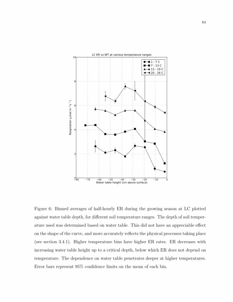
64
Figure 6: Binned averages of half-hourly ER during the growing season at LC plotted
against water table depth, for di↵erent soil temperature ranges. The depth of soil temper-
ature used was determined based on water table. This did not have an appreciable e↵ect
on the shape of the curve, and more accurately reflects the physical processes taking place
(see section 3.4.1). Higher temperature bins have higher ER rates. ER decreases with
increasing water table height up to a critical depth, below which ER does not depend on
temperature. The dependence on water table penetrates deeper at higher temperatures.
Error bars represent 95% confidence limits on the mean of each bin.

65
Figure 7: ER plotted against water table height for LC (•), WC (�), and Sylvania (⌃).
The plot is a binned average of growing-season ER, calculated from half-hourly data.
Each point is the mean of a water table range containing an equal number of points.
WC and Sylvania, the upland forest sites, are plotted against LC WT for comparison.
The wetland site exhibits a large decrease in ER with higher WT at a level about 30 cm
below the surface. WC and Sylvania, the upland sites, do not show the same relationship
between ER and water table, indicating that the dependence in the wetland site is not a
statistical artifact. Error bars represent 95% confidence limits on the mean of each bin.

66
Figure 8: Yearly average GEP plotted against WT averaged over the period of each
year when soil temperature was greater than 0�C at LC (•), WC (�), and Sylvania (⌃).
The upland sites WC and Sylvania are plotted against LC water table for comparison.
Wetland GEP is highly correlated with water table (correlation coe�cient –0.94), while
upland GEP has no significant correlation with wetland water table. Yearly average
wetland GEP increased by over 20% over the record.

67
Figure 9: Yearly-averaged NEE at Lost Creek, Willow Creek, and Sylvania as a function
of Lost Creek warm period WT. NEE was not correlated with LC water table at any of the
sites. The relationships between NEE and whole-year average WT were not materially
di↵erent.

68
Figure 10: Weekly-average growing season evapotranspiration (solid line), and water
table (dashed line) at Lost Creek. Evapotranspiration decreased as water table declined.
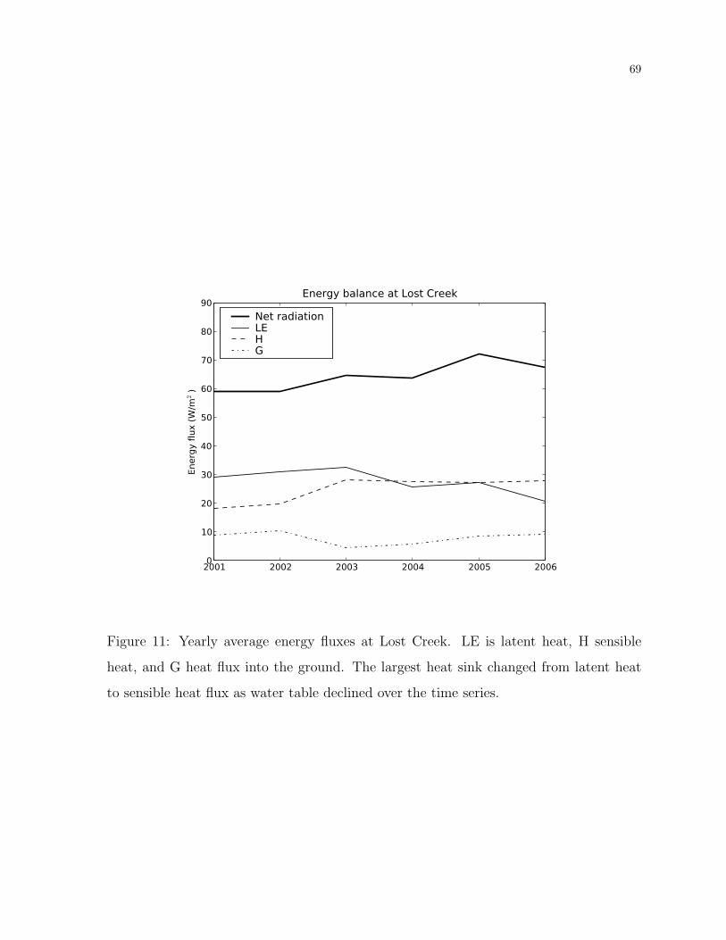
69
Figure 11: Yearly average energy fluxes at Lost Creek. LE is latent heat, H sensible
heat, and G heat flux into the ground. The largest heat sink changed from latent heat
to sensible heat flux as water table declined over the time series.

70
Figure 12: Yearly average evaporative fraction (Eq. 2) as a function of warm-period
water table at LC. The dashed line indicates the level where latent heat flux and sensible
heat flux are equal. EF declined as water table declined (r = 0.975) and EF crossed
below the 0.5 level, indicating that sensible heat flux became a larger part of the energy
budget than latent heat flux.

71
Figure 13: Yearly Lost Creek water use e�ciency (defined here as the ratio between
evapotranspiration and GEP) as a function of WT averaged over the period of each year
when soil temperature was greater than 0�C. Evapotranspiration decreased as the water
table declined while GEP increased, resulting in a net increase in WUE. The correlation
coe�cient is –0.91.

72
Figure 14: ER at the three wetland sites. LC (shrub fen) is circles, WF (sedge and grass
fen) is squares, and SF (bog) is triangles.

73
Figure 15: GEP at the three wetland sites. LC (shrub fen) is circles, WF (sedge and
grass fen) is squares, and SF (bog) is triangles.

74
Figure 16: Net ecosystem CO2 exchange at the three wetland sites. LC (shrub fen) is
circles, WF (sedge and grass fen) is squares, and SF (bog) is triangles.

75
Figure 17: Latent and sensible heat fluxes as a function of warm-period water table
at the three wetland sites. Black symbols are latent heat fluxes and open symbols are
sensible heat fluxes. Circles are LC (shrub fen), squares are WF (sedge and grass fen),
and triangles are SF (bog). Latent heat flux was correlated with water table across the
sites (r = 0.71, p = 0.005), while sensible heat flux was not significantly correlated with
water table (r = 0.04)

76
Table 1: Yearly average measurements for LC. NEE, ER, and GEP are average fluxes
in µmol m�2s�1, precipitation is total mm for each year, and water table (WT) is in cm
above soil surface.
Year NEE ER GEP WT Total precip Average T (C)
2001 -0.17 1.81 1.98 -8.05 865 5.61
2002 -0.25 1.56 1.76 -8.67 965 4.86
2003 -0.25 1.91 2.12 -32.84 692 4.11
2004 -0.18 2.15 2.32 -27.72 814 4.04
2005 -0.27 2.06 2.33 -33.79 790 5.74
2006 -0.21 2.16 2.37 -39.25 665 6.09