1

A Bayesian Approach to the Analysis of Split-Plot Product Arrays

and Optimization in Robust Parameter Design

Abstract

Many robust parameter design (RPD) studies involve a split-plot randomization structure

and to obtain valid inferences in the analysis, it is essential to account for the design

induced correlation structure. Bayesian methods are appealing for these studies since they

naturally accommodate a general class of models, can account for parameter uncertainty

in process optimization, and offer the necessary flexibility when one is interested in non-

standard performance criteria. In this article, we present a Bayesian approach to process

optimization for a general class of RPD models in the split-plot context using an

empirical approximation to the posterior distribution of an objective function of interest.

Two examples from the literature are used for illustration.

KEY WORDS: Bayesian Predictive Density; Generalized Linear Mixed Models; Hard-

to-Change Factor; Markov Chain Monte Carlo; Process Optimization; Response Surface;

Restricted Randomization.

2

Introduction

In many robust parameter design (RPD) applications, the response of interest

follows a non-normal distribution. For instance, Lee and Nelder (2003) utilize Poisson

regression to estimate the relationship between the number of solder defects and eight

design variables (5 control factors and 3 noise factors). Myers, Brenneman and Myers

(2005) demonstrate the use of gamma regression in modeling the relationship between

resistivity and four design factors (3 control and 1 noise factor) using data from a wafer

etching process in semiconductor manufacturing.

Quite often in RPD, the designed experiment is a crossed or product array (i.e., a

design for the noise factors crossed with a design in the control factors). Although there

are times when a completely randomized design (CRD) is appropriate for these

experiments, a split-plot design (SPD) can be easier and more cost efficient to implement

when hard/difficult-to-change factors exist. Even when hard-to-change factors do not

exist, Box and Jones (1992) point out that SPD’s are often more efficient than CRD’s

especially when the noise factors are in the outer array. Goos et al. (2006), Wolfinger and

Tobias (1998), and Ganju and Lucas (1997) note that the induced correlation structure

from a SPD must be accounted for in the analysis to obtain valid statistical inferences.

Wolfinger and Tobias (1998) suggest the use of linear mixed models for RPD SPD’s with

normal responses but do not discuss prediction. Robinson et al. (2004) advocate the use

of generalized linear mixed models (GLMMs) for industrial SPD’s with non-normal

responses. Robinson et al. (2009) propose Bayesian methods for the analysis of SPD’s

with non-normal responses.

Several uses of Bayesian methods for RPD have appeared in the literature but all

assume complete randomization of the experimental run order. Chipman (1998) propose

a Bayesian approach for product arrays. Miro-Quesada, Del Castillo, and Peterson (2004)

present a Bayesian approach using the posterior predictive distribution for multiple

response optimization. Rajagopal, Del Castillo and Peterson (2005) extend the work of

Miro-Quesada et al. (2004) to cases in which the practitioner seeks an RPD solution

robust to uncertainty in the process model by using Bayesian model averaging. Bayesian

approaches are appealing in RPD since (a) they allow for uncertainty in parameter

estimation to be accounted for when obtaining an optimal solution in the control factor

3

space; (b) process quality can be optimized in terms of a variety of performance criteria

such as conformance probabilities and other more useful characteristics of the response

distribution than being restricted to the process mean and variance; and (c) the approach

can handle a wide class of error distributions in a straightforward manner.

In this article, we define a general class of models for product array robust design

experiments with a split-plot randomization structure. We then develop a Bayesian

approach for modeling the data along with an optimization approach using an empirical

approximation to the posterior distribution of a user-defined objective function. The

methodology is illustrated with two examples from the literature and we consider some

non-standard performance criteria in characterizing the underlying process.

Model Formulation and Examples

For an exponential family member response observed from a split-plot

experiment, we consider an extended class of generalized linear models which include

random effects. Let y be an N1 vector of responses (N denoting the total number of

subplot runs), X an Np matrix of whole plot and subplot model terms, denote the

associated p1 vector of fixed-effects regression parameters, Z an Nw model matrix for

the random effects and the corresponding w-vector of random effects. Models under

consideration contain two parts:

1. Conditional on the random effect , the response distribution is a member of

the exponential family of distributions with

| , |E Var V y y ,

where is the dispersion parameter and V is the variance function. The linear

predictor is given by

X Zg .

Here, the link function, g , is chosen to be monotonic and differentiable.

2. The random effects in are assumed i.i.d. according to some specified

probability distribution.

4

Normal Response Example

Box and Jones (1992) consider an example where the manufacturer seeks the best

recipe for a box cake mix. In the example there are three control factors: X1 = flour, X2 =

shortening and X3 = egg powder, coded in the ranges -1 to +1. The manufacturer is

concerned that random fluctuations in cooking time, Z1, and cooking temperature, Z2, in

home ovens (both treated as noise factors with 2 levels codes as -1 and +1) may result in

cake flavor that is too variable. In order to develop a robust cake recipe, a 22 factorial

design in the noise factors is crossed with a 23 factorial design in the control factors. For a

fixed level combination of Z1 and Z2, eight cakes are baked, each with a different

combination of X1, X2 and X3 levels and the run order of the control factor combinations

are randomized. Note that in this experiment, the noise factors are in the whole plots,

while the control factors are changed within the whole plots.

Consistent with Box and Jones (2002), we assume 2 2| , ~ ,ij ij ijy N , where

ijy denotes the average cake quality (i.e., averaged across a panel of judges who each

ranked taste from 1-7) for the jth

cake baked at the ith

level combination of Z1 and Z2

1,...,4; 1,...,8i j . Also consistent with Box and Jones, we treat the response as

continuous since ordinal scores are averaged over a panel of judges. While Box and Jones

focused upon treatment comparisons we consider response optimization and fit a model

with an identity link i.e., | |ij i ijg

. Thus, the linear predictor is given by

ij|

i

ij| x

ij

' i, (1)

where each x

ij

' denotes a 115 vector of model terms consisting of the intercept, the two

noise main effects, six control factor only effects (i.e., 3 main effects and 3 two-factor

interactions), and the six control-by-noise two-factor interactions. The ’s are the

associated fixed-effects model parameters while the i represent the whole-plot error

terms and are assumed to be i.i.d. Normal 20 , . Relating the model in (0) to the

general formulation, we have g , y denotes the 321 vector of responses starting

with the eight observations in the first whole plot and so on, Z is a 324 classification

matrix of ones and zeros where the klth

entry is a one if the kth

observation (k=1,…,32)

5

belongs to the lth

whole plot (l=1,…,4). The i

comprise the 41 vector of random

effects, , and the rows of the 3215 model matrix X are formed by x

ij

' .

Gamma Response Example

Robinson et al. (2004) consider data from a film manufacturer in which the

investigator wishes to study the effects of six factors (three mixture components [X1, X2,

X3] and three process variables [p1, p2, and p3]) on film quality. We assume for this

application that the process variables represent environmental variables whose

fluctuations in the process cause unwanted variation in the response. A product array with

the mixture design in the control factors serving as the outer array and a 23-1

design in the

process variables as the inner array was conducted. Note that there is potential for

confusion with the terminology of the experiment, since we need to clarify both the RPD

and the split-plot pieces of the design. In RPD, the control factors are traditionally labeled

as being in the inner array and noise factors in the outer array, and yet for this

experiment, control factor levels were randomized at the whole plot level and the noise

factor levels were randomized at the subplot level. Note that this experimental set-up

differs from the first example where the noise factor levels were varied within the whole

plots. The goals of this experiment were to: (a) examine the impact of the mixture

variables on response quality; (b) study the contribution of the noise factors to process

variance; and (c) determine optimal settings for the mixture variables. In the experiment,

five distinct formulations of the mixture variables were used to produce a total of 13

batches (one batch=one roll). Upon production of a roll of film with a given setting of the

mixture variables, four pieces of the roll were randomly assigned according to a 23-1

design in the process variables.

Consistent with Robinson et al. (2004, 2009) and Lee, Nelder and Park (2010), we

assume | , ~ ,ij ij ijy Gamma , where ijy denotes the film quality for the j

th piece of

film from the ith

roll. The following parameterization of the gamma density is assumed,

1 y

y

y ef y

. (2)

Using the model of Robinson et al. (2004, 2009), a log link i.e., gij i ij i

ln

| | ,

with linear predictor

6

'

3 3 2 3

12 1 2

1 1 1 1

ij i ij i ij i

b b ij ij ij c ij c ij bc b ij c ij i

b c b c

ln

x x x p x p

x

, , , , , , ,

| |

, (3)

is fit. Note that the linear predictor in (0) does not include an intercept since we are fitting

a Scheffé model for mixture experiments and only a subset of the total number of

possible two factor interactions were of interest. In (3), the ’s are for the first and

second order mixture/control factor terms, the ’s are for the linear process/noise terms,

and the ’s represent the mixture-by-process/control-by-noise interactions. Relating the

model in (0) to the general formulation, we have lng , y denotes the 521 vector

of observations starting with the four observations from the first roll and so on, Z is a

5213 classification matrix of ones and zeros, where the klth

entry is a one if the kth

observation (k=1,…,52) belongs to the lth

roll (l=1,…,13). The rows of the 5213 model

matrix X are formed by '

ijx for each observation.

Bayesian Inference

Let denote the vector of model parameters. The Bayesian inferential approach

combines prior information about with the information contained in the data. The

prior information is described by a prior density, , and summarizes what is known

about the model parameters before data are observed. The information provided by data

is captured by the data sampling model, |fy y , known as the likelihood. The

combined information is described by the posterior density, | y . We evaluate the

posterior density using Bayes' Theorem [Degroot (1970) p. 28] as

( | ) ( | ) ( )f y y .

For the cake mix example, ' ' ',  ,, , where ' is the 115 vector of

regression coefficients, 'δ is the 14 vector of random effects used to model the outer

array error term, is the standard deviation of the random effects distribution, and is

the normal error shape parameter. The likelihood |fy y has the form

7

4 8

1 1

( | ) ( | , )y ij iji j

f f y

y y ,

with ij given in (0), where ( | , )y ij ijf y is a normal density. We see from (0) that

ij also depends on x

ij

' , ' , and i . The prior density, , has the form

() fi(i

i1

4

|2)

f

j( j

j1

15

)

f( ) f

( ) ,

where ( )f is the Normal(0, 2

) density assumed for the random effects, i . For the

regression coefficients (the 'j s ), we use the following diffuse but proper prior

distributions: Normal(0,10002). For

, we use the diffuse prior distribution Uniform(0,

10). For , we use the informative prior distribution Gamma(625,10000). An

informative prior is needed here since there is no replication of whole plots, and hence

the observed data do not contain information about both the interaction between time and

temperature and the whole plot variability.

For the film manufacturing example, ' ' ', , , , where is the gamma

shape parameter, ' is the 113 vector of regression coefficients given in (3), 'δ is the

113 vector of random roll effects, and is the standard deviation of the random effects

distribution. The likelihood |fy y has the form

13 4

1 1

( | ) ( | , / )y ij ij iji j

f f y

y y ,

with fy ( yij | ,ij ) from (0) and ij given in (0). From (0), it is evident that ij depends

on'

ijx ,β , and i . The prior density, , has the form

13 132

1 1

( ) ( | ) ( ) ( ) ( )i ji j

i j

f f f f

,

where ( )f is the Normal(0, 2

) density assumed for the random roll effects i . For the

regression coefficients (the 'j s ) and , we use the diffuse but proper prior

8

distributions: Normal(0,10002) and Uniform(0,100), respectively. For , we use the

diffuse prior Uniform(0,100) distribution as suggested by Gelman (2006).

When the form of the posterior density is well known, the posterior distribution

can be obtained in closed form. For more general forms of the posterior density, we can

approximate the posterior distribution via Markov chain Monte Carlo (MCMC) [Gelfand

and Smith (1990), Casella and George (1992), Chib and Greenberg (1995)]. The MCMC

algorithm produces samples from the joint posterior distribution of by sequentially

updating each model parameter conditional on the current values of the other parameters.

To analyze both examples, we used WinBUGS [Spiegelhalter, Thomas, Best, and

Lunn (2004)]. For the cake mix data, summaries of the joint posterior draws of are

given in Table 1, and are based on two chains of length 100,000 thinned to every 20th

draw, i.e., totaling 10,000 draws. A similar summary for the film example is given in

Table 2. Note that in the cake mix example there are no whole plot replicates, so the

marginal posterior distribution of the whole plot error variance is essentially the chosen

informative prior. For the film example, there are several whole plot replicates, so that

the whole plot error variance can be estimated; thus, the data can update the prior.

To assess convergence of the MCMC algorithms and goodness-of-fit of the

models to the data, several diagnostics were considered. We begin with diagnostics for

the cake mix example. To assess the convergence of the MCMC algorithm, trace plots of

the MCMC chains, such as those in Figure 1, work well. Figure 1 contains the trace plots

of the MCMC chains for the first four regression coefficients in the cake mix example.

Here, only one of the two chains is shown, and the pictured chain is thinned to every

100th

iteration instead of every 20th

. Figure 1 shows that convergence for the four

parameters has occurred by iteration 10,000, and that they are mixing well. Trace plots

for the other model parameters (not shown) all lead to similar conclusions. See Gelman

et al. (2004, Section 11.6 pp. 294-299) for more discussion of MCMC convergence

diagnostics.

The overall fit of the model to the data can be examined by the Bayesian 2

goodness-of-fit test (Johnson, 2004). The test proceeds as follows:

1. Divide the interval [0, 1] into N0.4

=320.4

=4 bins (as recommended by Johnson

(2004)), and set each bin count to zero.

9

2. For a given MCMC draw of Θ, calculate the cumulative probability of ,

, and . Here, F is a normal

cumulative distribution function.

3. If , the count of bin 1 is increased by 1. If , the

count of bin 2 is increased by 1, etc.

4. Compute the standard statistic for comparing the observed bin counts to the

expected bin counts, N/4=32/4=8.

5. Compare the statistic to the 95th

percentile of the distribution where the

degrees of freedom are computed as 3=4-1.

6. Repeat 1-5 for all 10,000 (2 chains 5,000 draws per chain) draws of .

If approximately 95% of the tests fail to reject that the observed bin counts are consistent

with the expected bin counts, there is no evidence of lack-of-fit. That proportion for the

cake mix example is 94.14%.

To check the assumption of normal random effects, for each posterior draw of ,

, an envelope based the corresponding draw of is created. The number

of draws, , that falls within its corresponding envelope summarizes the

appropriateness of the normal assumption for the random effects. An envelope is created

by the following procedure:

1. Generate 1,000 sets of 4 deviates.

2. Order each set.

3. Calculate the 0.013/2 and 1-0.013/2 percentiles of each order statistic since

0.9874

0.949.

A draw of , , is said to fall within its envelope if its order statistics fall

within their corresponding intervals. If approximately 95% of the , ,

draws fall within their corresponding envelope, the normal assumption for the random

effects is tenable. The percentage for the cake mix example is 95.12%.

Lastly, we consider the conditional normality of the response, , by examining

the residuals, . Using the posterior distribution of , we create a normal

q-q plot from the medians of those distributions. The plot is given in Figure 2, and it

suggessts the conditional normality of the response is reasonable.

10

Similar diagnostics were considered in the film manufacturing experiment, and

they imply no problems with the convergence or mixing of the MCMC chains or the fit of

the model to the data. One difference between the diagnostics for the cake mix

experiment and the film manufacturing experiment is that deviance residuals, instead of

raw residuals, are used for the film manufacturing experiment because the response is

assumed to be conditionally gamma instead of normal. Also for the film manufacturing

experiment, we may consider a different diagnostic for assessing the assumption of

normal random effects. Specifically, we create a normal q-q plot from the posterior

means of , , which are given in Table 2. The plot is shown in Figure 3,

and it implies the normal assumption for the random effects is reasonable. Such a plot in

the cake mix experiment is not as useful since there are only four random effects.

Prediction, Performance Criteria and Optimization

Posterior Predictive Density and Performance Criterion

The primary goal of RPD is to find levels of the control factors which lead to

desirable process quality results. Thus, we wish to optimize an appropriate characteristic

of the response distribution under future production conditions. Inference regarding

unobserved values of the response generally focuses upon characteristics of a posterior

predictive density where the density incorporates all potential sources of uncertainty.

However, we take a slightly different approach. Let newy denote a new, observed value

of the response from the process, new an unobservable random effect associated

with newy , cx a combination of control factors, and nx a combination of noise factor

levels. We consider the following density

| ,  , , |

= | , , |

new n

new n

new c new new n c n new

new new c n new n n new

f y f y

f y f f

x

x

x x x x

x x x x,

where | , ,new new c nf y x x is a normal density in the first example and a gamma

density in the second example, |newf is a univariate normal density, and nf x is

a user-specified multivariate normal density representing anticipated random fluctuations

11

of the noise factors during the process. Note that | , new cf y x incorporates the

variability associated with random fluctuations of the noise factors (through nf x ), the

variability associated with a new whole plot effect (through |newf ) and the

variability associated with the new observed responses (through | , ,new new c nf y x x ).

Also, | , new cf y x is related to the posterior predictive density, | , new old cf y y x , since

| , |new old c new c oldf y f y f y x x y

,

and oldy denotes the vector of observed data. The posterior predictive density, which

integrates over the uncertainty from estimating the model parameters, is the focus of

Miro-Quesada, Del Castillo and Peterson (2004) who discuss process optimization for

completely randomized designs with normal responses. We choose to focus on the

distribution of | , new cf y x because it summarizes what we expect to see under future

regular process conditions, and allows for greater flexibility in specifying performance

criteria or objective functions for the optimization. Specifically, let the function , ch x

denote a characteristic of the density in (4). This function is chosen to represent an

important aspect of the response upon which process optimization should be based.

Given that we have variability from many sources as well as uncertainty from the

parameter estimation, we wish to examine what range of values of , ch x are possible

across the probable parameter values. For example, in the film example, guarding against

a worst case scenario for the proportion of high quality film could be more important to

the practitioner than estimating the proportion of high quality film using the posterior

predictive density. Quite often in RPD, optimization focuses on a criterion such as

squared error loss. In the cake example, high taste scores (close to the maximum of 7)

are most desirable. Thus, one might wish to find   cx such that a property of the posterior

distribution of

| ,

2, 7 * 7

new cc y new newh E y I y

xx

is minimized, where

12

| ,

2 2| ,7 * 7 7 * 7

ne

new c

w

y new new new new new c new

y

E y I y y I y f y dy x

x

  .

In the definition of , ch x above, we include the indicator function so as not to

penalize any predicted response greater than 7, which is the maximum possible average

score for taste.

For the film example, Robinson et al. (2009) suggest that film pieces whose

quality exceeds 150 represent premium grade film. As such, it might be desirable to find

  cx such that the exceedence probability Pr 150| ,,  newc ch y x x is maximized,

using

150

Pr 150| , | ,

new

new c new c new

y

y f y dy

 x x   .

General Description of Optimization Algorithm

To investigate robust values of cx , we evaluate properties of the posterior

distribution of , ch x over a grid of cx points. Consider a single point in the grid of

cx values, say 0

cx . To evaluate properties of the posterior distribution of 0, ch x , we

first obtain a sample of MCMCN 's from oldf y using WinBUGS, and a sample of

NoiseN observations of nx from the user-specified ( )nf x . Then, for each of the

MCMC NoiseN N , n x  pairs, we sample a value of new from the appropriate distribution.

For our examples, this is the univariate normal. For each of these MCMC NoiseN N

,n newx triples, we sample a newy value from the appropriate normal (first example)

or gamma (second example) distribution. Since noiseN of these newy values are generated

from the same posterior draw, say 0 , we can estimate 0 0, ch x . For example, if

00 0 0Pr 150| ,,  newc cyh xx ,

0 0 0

1

1Pr 150| ,  150

noiseN

i

new c new

inoise

y I yN

x ,

13

where 0i

newy is the thi value of newy generated according to 0 for a particular

choice of cx . This process gives MCMCN posterior samples of 0, ch x , thereby enabling

the estimation of quantities such as 0,old

cE h

xy|

, 0,old

chVar

y

x|

, and the 5th

,

10th

, and 50th

posterior percentiles of the posterior distribution of 0, ch x , for instance.

The median gives us the center of the distribution while the 5th

and 10th

percentiles give

lower bounds on 0, ch x . If we had focused on the posterior predictive distribution,

then only a single summary, such as the mean or an exceedance probability is possible.

With the proposed approach, understanding the characteristics of the distribution of

0, ch x induced by the uncertainty in is possible, and allows for greater flexibility to

select a most relevant attribute of the distribution.

Examining these quantities over a grid of cx values provides the opportunity to

choose cx candidates that are robust to changes in nx . Note that maximizing

0150| , Prold

new cE y

xy

|

over values of cx , is equivalent to maximizing

Pr( 150 | ,  )new old cy y x over values of cx , since

0 0 0

150

0

150

0

150| , | , ,

( , | , )

150| .,

Pr

Pr

oldnew

new

new c new c new old c

y

new old c new

y

new old c

E y f y y f

f y y

y

x x y xy

y x

y x

|

Also note that optimizing Pr | , new old cy A y x over values of cx was the approach of

Miro-Quesada, Del Castillo and Peterson (2004) but they did so for situations where

| , new old cf y y x exists in closed form.

To facilitate a fair comparison for each cx in the grid, we use the same sample of

MCMC NoiseN xN n x pairs for each cx in the grid. Further, when the analyses in both

14

examples were re-done, using different samples of the

NMCMC NNoise n x pairs, the

results were essentially unchanged.

Results for the Examples

Cake Mix Experiment Results

Using the sample of NMCMC posterior ' s obtained from WinBUGS, we now seek

to find the optimal combination of control factors (Flour, Shortening and Eggs) to

minimize the expected squared loss from the target taste value of 7. These settings are

chosen to be robust to variations in the cooking time and temperature which are not as

tightly controlled when consumers bake the cake compared to the laboratory

environment. Similar to other RPD applications, we assume that the distribution of the

coded noise variables (cooking time and temperature) in the less controlled consumer

environment is appropriately modeled with a bivariate normal distribution with mean (0,

0) and variance 2I .

When we examine the optimizations based on different criteria from the posterior

distribution of 2

, 7 * 7c new newh E y I y

x over the design region, we see that

different settings are identified as best depending on the criterion considered. Table 3

shows various locations of optima along with their respective optimum values depending

upon which characteristic of the posterior of , ch x one is interested in optimizing

with respect to. Note that all optimal settings have Flour and Eggs set to their maximum

amount (1 in the coded factors), but the amount of Shortening to be included varies by

criterion. The optimization actually proceeded in two stages. In the first stage,

is optimized over the grid . In the second stage,

optimization is performed over the finer grid . By considering

several properties of the posterior of , ch x , rather than just a single summary, we

are able to gain a more detailed understanding of how to best optimize the process. For

example, the smallest mean and median of the posterior for , ch x occurs at the

control factor setting of (1, 1, 1) with corresponding values 2.93 and 2.83, respectively.

The optimal control factor setting shifts more towards middle values of Shortening to

15

optimize the tail of the posterior distribution of , ch x . Specifically, the 90th

percentile

is minimized at the control factor setting (1, 0.8, 1) with a value of 4.08 and the minimum

95th

percentile is 4.44 at the control factor setting (1, 0.6, 1). Hence if the manufacturer

wishes to optimize the typical taste characteristic for the consumer, then the optimal

setting should be chosen as (1, 1, 1). However, if it is a priority for the company to make

sure that very few consumers experience poor taste, then the setting of (1, 0.8, 1) or (1,

0.6, 1) should be considered as best.

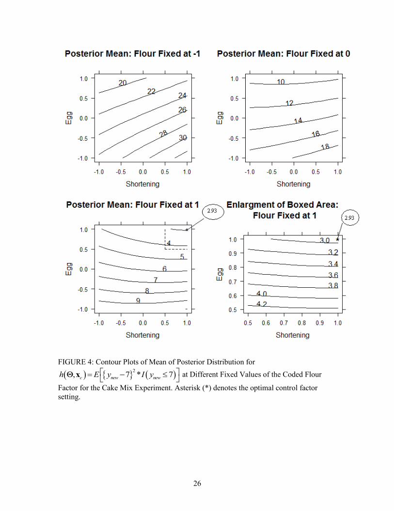
Figure 4 shows the contour plot of the mean of the posterior distribution of

, ch x across the design region. The first three sub-figures show contour plots for

different fixed values of Flour across the range of design Egg and Shortening factors. The

final sub-figure shows an enlargement of the optimal corner of the design region with

more detailed contours.

Figure 5 shows contour plots for different attributes of the posterior distribution of

, ch x with Flour fixed at a value of 1. Examining the plots, we see that the shape of

the contour lines changes for the different percentiles of the posterior, with the median

optimized in the corner of the design space, while the optimum control factor settings for

tail percentiles favors smaller amounts of Shortening. While there are differences in the

global optimum, we can see that the optimal RPD operation setting does not change the

amounts of Flour and Eggs. Given the flat contour lines in the Shortening direction for

Flour and Eggs at their maximums, these differences in the optimal settings represent

some alternatives which perform quite well across a range of different distributional

characteristics.

Finally, we compare the results of our optimization to those that would have been

obtained if we had used a criterion of maximizing the proportion of the posterior

predictive distribution above a certain threshold using methodology similar to what was

outlined in Miro-Quesada et al. (2004). In this case, if one maximizes the proportion of

responses above the taste score thresholds of 6 and 6.5 according to the posterior

predictive distribution, similar but not identical results are found compared to those

above. Optimal control factor settings for maximizing Pr 6 |new oldy y and

Pr 6.5|new old

y y along with the corresponding values are found in the last two rows of

16

Table 3. In the case of the posterior predictive distribution, the proportions of Flour and

Eggs are maintained at their maximum values, but the optimal setting of Shortening is at

its low level. The global best control factor setting is (1, -1, 1), with 37% and 24% of the

distribution predicted to fall above each threshold, respectively. Based on these results, it

is clear that the Flour and Eggs settings should be maximized, while the criterion for

optimizing determines the value of the Shortening.

Film Manufacturing Experiment Results

We now consider RPD optimization for the film manufacturing example using the

sample of NMCMC posterior ' s obtained from a Bayesian analysis of the data in

WinBUGS. The goal of this analysis is to determine the control/mixture factor level

combination [X1, X2, X3] which maximizes the proportion of high quality film given the

unwanted variation from the process variables [p1, p2, p3] in the less controlled

production environment. As with other RPD applications, we assume that the coded noise

factors are from a trivariate normal distribution with mean (0, 0, 0) and variance, 3I . The

optimal settings and corresponding values based on different criteria from the posterior

distribution of Pr 150| ,,  newc ch y x x are summarized in Table 4. For all

summaries of the posterior of Pr 150| ,,  newc ch y x x , the goal is to find the

control factor settings resulting in maximization. We utilized a grid search to find the

optimal mean, median, 5th

and 10th

percentiles of the posterior distribution of , ch x .

As in the cake mix example, the optimization proceeds in two stages. In the first stage,

is optimized over the grid

. In the second stage, optimization is

over the finer grid . The

best mixture combination based on the mean of Pr 150| , new cy x is at

1 2 3( , , ) (0.5425,0.2575,0.2000)X X X . Figure 6 provides the contour plots of the mean

of Pr 150| , new cy x across the control factor space. Since the control factors are

mixture variables in this experiment (constrained to sum to one), the entire design region

for the outer array is shown in two dimensions ( 2 3 and X X ) with 1 2 31 - X X X

17

inferred. Figure 6(a) shows the control factor design space, while Figure 6(b) shows an

enlargement of the region with the optimum, shown with the dashed line in Figure 6(a).

The surface corresponding to the mean of the posterior distribution of , ch x is quite

smooth with a single maximum on the boundary of the space. We note that this solution

is similar to the approach of Miro-Quesada et al. (2004) as it maximizes the proportion of

the posterior predictive distribution above 150. For our implementation, we have

estimated the value using the MCMC draws, rather than finding a closed form expression

for the quantity.

Alternately, we consider different percentiles of the posterior of , ch x for

selecting the best production recipe for film. The settings of the optimum based on the

50th

, 5th

and 10th

percentiles of the posterior distribution of , ch x are also given in

Table 4. All of the identified optima have 3 0.2X , but the proportions of 1 2 and X X

differ depending on the criterion considered. For the median, the estimated proportion of

high quality film is 0.886, with two distinct settings, 1 2 3( , , ) (0.535,0.265,0.200)X X X

or (0.52,0.28,0.20) , producing this value. The median or mean of , ch x ’s posterior

distribution represent “typical” proportions of high quality film under expected noise

condition variation, while the lower percentiles (5th

and 10th

) monitor the “worst case”

proportion of high quality film under the uncertainty in the model parameters. By

considering the proportion of high quality film in the tails of the posterior distribution

(0.623 and 0.719 for the 5th

and 10th

percentiles, respectively), we gain a more realistic

assessment of what proportions might be observed during regular production. The choice

of which metric to select depends on whether we want to optimize typical proportions of

high quality film or determine a setting where we can be very confident of attaining at

least a certain proportion. Figures 4, 5 and 6 shows contour plots for the median, 5th

and

10th

percentiles, respectively, across the design region. The second sub-figure 10 in each

plot shows an enlargement of the contour plot around the optimum for the area denoted

by the dashed line in the first sub-figure.

As we protect more against the tail of the posterior distribution, the 2X

proportion decreases to 0.2050 (with1X increasing to 0.5950). Quantifying the trade-off

18

in both settings and the proportion of high quality film expected can help managers make

more informed decisions about what to expect during regular production. Table 5 shows

the values of the different criteria associated with , ch x for two settings which

correspond to the optimal settings for the median and 5th

percentile criteria. If we choose

based on the median or “typical proportion”, then an optimal setting is

1 2 3( , , ) (0.535,0.265,0.200)X X X . However, if we used the 5th

percentile as a

conservative measure to almost guarantee at least a certain proportion of high quality

film, then the optimal setting is 1 2 3( , , ) (0.595,0.205,0.200)X X X . When we consider

the results in Table 5, we see that while the optimum setting shifts slightly depending on

the chosen criterion, none of the competing criteria perform too badly at the optima of

another. By considering the entire posterior distribution of Pr 150| , new cy x , and

matching its characteristics to aspect of production on which we wish to focus, we can

make a more informed choice for how to optimize the process.

Conclusions and Discussion

In this paper we present a method for finding optimally robust settings in the

control factor space for different characteristics of the posterior distribution of an

objective function. The Bayesian approach allows flexible objective functions for a very

general class of models. In the two examples, the responses were normal and gamma

distributed; the proposed methodology easily handles other response distributions such as

the Weibull and lognormal distributions for continuous responses and the binomial and

Poisson distributions for discrete responses. The methods presented were compared to the

optimization based on the posterior predictive distribution described in Quesada et al.

(2005) and shows the two approaches are related if the mean of the posterior distribution

is selected. In other cases, the more general new approach allows different functions of

the model parameters to be considered, and different attributes of the posterior

distribution to be utilized. This flexibility allows the user to specify an attribute of the

distribution that most realistic summarizes what is of primary interest in the experiment.

Assessing the robustness of the optimization results across different potential attributes is

straightforward and allows direct comparison of trade-offs.

19

Using the optimization algorithm, it is straightforward to substitute more

complicated noise variable structures, including correlations, into the optimization. For

example, in the film experiment, the distribution of the coded noise factors in the

production environment could have been replaced with a multivariate normal distribution

with mean (0,0,0) and variance

12 13

12 23

13 23

1

1

1

, with no additional complication other

than how to sample the noiseN values.

In the cake example, there were no whole plot replicates to allow estimation the

variance of 2

from the data. Hence the prior distribution provided the needed

information to complete the analysis. In general, the authors feel that whenever possible

designs should be selected with adequate whole plot replication to provide some

confirmation of the range of values for 2

. However, when no replication is possible, the

Bayesian approach allows incorporating external knowledge of uncertainty into the

analysis.

Acknowledgements

We thank Derek Bingham of Simon Fraser University and Alyson Wilson of Iowa State

University for helpful discussions.

References

Box, G.E.P. and Jones, S. (1992). “Split-Plot Designs for Robust Product Experimentation”.

Journal of Applied Statistics, 19, pp. 3-26.

Casella, G. and George, E. (1992). “Explaining the Gibbs Sampler”. The American

Statistician, 46, pp. 167-174.

Chib, S. and Greenberg, E. (1995). “Understanding the Metropolis-Hastings Algorithm”.

The American Statistician, 49, pp. 327-335.

Chipman, H. (1998). “Handling Uncertainty in Analysis of Robust Design Experiments”.

Journal of Quality Technology, 30, pp. 11-17.

DeGroot, M.H. (1970). Optimal Statistical Decisions. New York: McGraw-Hill.

Ganju, J. and Lucas, J.M. (1997). “Bias in Test Statistics when Restrictions in

Randomization are Caused by Factors”. Communications in Statistics: Theory and

Methods, 26, pp. 47-63.

Gelfand, A.E. and Smith, A.F.M. (1990). “Sampling-Based Approaches to Calculating

20

Marginal Densities”. Journal of the American Statistical Association, 85, pp. 398-

409.

Gelman, A. (2006). “Prior Distributions for Variance Parameters in Hierarchical

Models”. Bayesian Statistics, 1, pp. 515-533.

Gelman, A., Carlin, J.B., Stern, H.S., and Rubin, D.B. (2004), Bayesian Data Analysis,

Second Edition, Chapman & Hall/CRC, Boca Raton, FL.

Goos, P., Langhans, I. and Vandebroek, M. (2006). “Practical Inference from Industrial

Split-Plot Designs”. Journal of Quality Technology, 38, pp. 162-179.

Johnson, V.E. (2004), “A Bayesian Chi-Square Test for Goodness-of-Fit,” Annals of

Statistics, 32, 2361-2384.

Lee, Y. and Nelder, J.A. (2003). “Robust Design Via Generalized Linear Models”.

Journal of Quality Technology, 35, pp. 2-12.

Lee, Y., Nelder, J.A., and Park, H. (2010), “HGLMs for Quality Improvement”. Applied

Stochastic Models in Business and Industry. DOI: 10.1002/asmb.840

Miro-Quesada, G., Del Castillo, E. and Peterson, J.J. (2004). “A Bayesian Approach for

Multiple Response Surface Optimization in the Presence of Noise Variables”.

Journal of Applied Statistics, 31, pp. 251-270.

Myers, R.H., Brenneman, W.A and Myers, W.R. (2005). “A Dual Response Approach

to Robust Parameter Design for a Generalized Linear Model”. Journal of Quality

Technology, 37, pp. 130-138.

Rajagopal, R., Del Castillo, E. and Peterson, J.J. (2005). “Model and Distribution-Robust

Process Optimization with Noise Factors”. Journal of Quality Technology 37,

pp. 210-222.

Robinson, T.J., Myers, R.H. and Montgomery, D.C. (2004). “Analysis Considerations in

Industrial Split-Plot Experiments with Non-Normal Responses”. Journal of

Quality Technology, 36, pp. 180-192.

Robinson, T.J., Anderson-Cook, C.M. and Hamada, M.S. (2009). “Bayesian Analysis of

Split-Plot Experiments with Non-Normal Responses for Evaluating Non-

Standard Performance Criteria”. Technometrics, 51, pp. 56-65.

Spiegelhalter, D., Thomas, A., Best, N. and Lunn, D. (2004). WinBUGS Version 1.4

User Manual.

Wolfinger, R.D. and Tobias R.D. (1998). “Joint Estimation of Location, Dispersion, and

Random Effects in Robust Design”. Technometrics, 40, pp. 62-71.

21

TABLE 1. Posterior Means, Standard Deviations, and Selected Quantiles for Regression

Coefficients 's , Random Effect Variance 2 and Subplot Variance 2

for the

Cake Mix Experiment

Quantiles

Parameter Mean Std. Dev. 0.025 0.5 0.975

Intercept 3.444 0.162 3.127 3.444 3.760

Time (t) 0.268 0.159 -0.048 0.269 0.575

Temp (T) 0.553 0.158 0.240 0.552 0.862

t

T 0.034 0.158 -0.278 0.034 0.338

Flour (F) 1.336 0.098 1.142 1.334 1.525

Shortening (S) -0.167 0.100 -0.366 -0.167 0.034

Egg (E) 0.603 0.098 0.409 0.604 0.797

F

S 0.098 0.099 -0.097 0.098 0.292

F

E 0.103 0.099 -0.092 0.103 0.302

S

E 0.065 0.099 -0.131 0.065

0.263

F

T 0.154 0.098 -0.039 0.155 0.347

F

t 0.004 0.098 -0.191 0.003 0.197

S

T -0.461 0.098 -0.656 -0.461 -0.268

S

t -0.110 0.099 -0.307 -0.108 0.084

E

T -0.015 0.099 -0.216 -0.015 0.182

E

t -0.043 0.098 -0.238 -0.043 0.151 2

0.310 0.133 0.145 0.280 0.644

2

0.062 0.002 0.058 0.062 0.067

22

TABLE 2. Posterior Means, Standard Deviations, and Selected Quantiles for Regression

Coefficients 's , Gamma Shape Parameter , Random Effects 'i s and Random

Effect Variance for the Film Manufacturing Experiment

Quantile

Effect Estimate Standard

Dev. 0.025 0.5 0.975

x1 6.169 0.4533 5.284 6.166 7.104 x2 4.035 0.4661 3.116 4.031 4.980 x3 1.265 0.9708 -0.7040 1.2780 3.213

x1

x2 10.550 2.8080 4.896 10.52 16.20 p1 -0.7074 0.5317 -1.7530 -0.7132 0.3595 p2 0.3728 0.5351 -0.6979 0.3743 1.417 p3 0.2952 0.5323 -0.7399 0.2886 1.344

x1

p1 1.217 0.7490 -0.2781 1.224 2.668 x2

p1 1.992 0.7506 0.5145 1.997 3.467 x1

p2 -0.2336 0.7551 -1.6920 -0.2372 1.283 x2

p2 -1.040 0.7582 -2.521 -1.039 0.4820 x1

p3 -0.4783 0.7477 -1.9690 -0.4745 0.9840 x2

p3 -0.1303 0.7524 -1.6230 -0.1255 1.333

4.835 1.167 2.861 4.717 7.412

1 0.1236 0.2550 -0.3563 0.1084 0.6605

2 -0.0301 0.2536 -0.5550 -0.0258 0.4871

3 0.1519 0.2558 -0.3296 0.1310 0.6943

4 0.0718 0.2560 -0.4311 0.05894 0.6122

5 -0.05651 0.2552 -0.6006 -0.04433 0.4486

6 -0.2264 0.2611 -0.7915 -0.2066 0.2395

7 -0.04031 0.2986 -0.6639 -0.0308 0.5665

8 -0.3423 0.2814 -0.9395 -0.3209 0.1273

9 0.2259 0.2643 -0.2499 0.2045 0.7945

10 0.1295 0.2582 -0.3637 0.1103 0.6803

11 0.2589 0.2579 -0.1818 0.2358 0.8286

12 0.04056 0.2991 -0.5474 0.03139 0.6818

13 -0.3369 0.2880 -0.9675 -0.3139 0.1369

0.3372 0.1606 0.06390 0.3212 0.7082

23

TABLE 3. Optimal Control Factor Settings and Values for Different Summaries of

2

, 7 * 7c new newh E y I y

x and the Posterior Predictive Distribution for the

Cake Mix Experiment

Minimizing summaries of 2

, 7 * 7c new newh E y I y

x

Setting

Value Flour Shortening Eggs

Mean 1.0 1.0 1.0 2.93

Median 1.0 1.0 1.0 2.83

90th

Percentile 1.0 0.8 1.0 4.08

95th

Percentile 1.0 0.6 1.0 4.44

Maximization Using Posterior Predictive Distribution

Pr 6 |new oldy y 1.0 -1.0 1.0 0.37

Pr 6.5|new old

y y 1.0 -1.0 1.0 0.24

TABLE 4: Optimal Control Factor Settings and Values for Different Summaries of

Pr 150| ,,  newc ch y x x for the Film Manufacturing Experiment

Setting

Value X1 X2 X3

Mean* 0.5425 0.2575 0.2000 0.854 (maximum)

Median 0.5350

0.5200

0.2650

0.2800

0.2000

0.2000

0.886 (maximum)

5th

Percentile 0.5950 0.2050 0.2000 0.623 (maximum)

10th

Percentile 0.5650

0.5500

0.2350

0.2500

0.2000

0.2000

0.719 (maximum)

* equivalent to the posterior predictive optimization of Quesada et al. (2005)

TABLE 5: Posterior Percentiles of Pr 150| ,,  newc ch y x x at Two Optimal

Control Factor Settings for the Film Manufacturing Experiment

X1 X2 X3 Mean Median 5th

%ile 10th

%ile Variance

0.5350 0.2650 0.2000 0.854 0.886* 0.614 0.716 0.015

0.5950 0.2050 0.2000 0.847 0.875 0.623* 0.714 0.014

* denotes best value across all control factor locations in design space

24

FIGURE 1: Trace Plots of the MCMC Samples for the First Four Regression

Coefficients in the Cake Mix Experiment.

25

FIGURE 2: Q-Q plot of the Medians of the Posterior Distributions of the Raw Residuals

for the Cake Mix Experiment.

FIGURE 3: Q-Q Plot of the Posterior Means of the Random Effects in the Film

Manufacturing Experiment.

26

FIGURE 4: Contour Plots of Mean of Posterior Distribution for

2

, 7 * 7c new newh E y I y

x at Different Fixed Values of the Coded Flour

Factor for the Cake Mix Experiment. Asterisk (*) denotes the optimal control factor

setting.

27

FIGURE 5: Contour Plots of Median, 90th

and 95th

Percentiles of the Posterior

Distribution for 2

, 7 * 7c new newh E y I y

x Coded Flour factor Set at 1 for

the Cake Mix Experiment. Asterisk (*) denotes the optimal control factor setting.

28

(a)

(b)

FIGURE 6: Contour Plots of Mean of Posterior Distribution for

Pr 150| ,,  newc ch y x x for the Film Manufacturing Example: (a) Entire Design

Region, (b) Enlargement of Region Close to Optimum Denoted by Dashed Line in (a).

Asterisk (*) denotes the optimal control factor setting.

29

(a)

(b)

FIGURE 7: Contour Plots of Median of Posterior Distribution for

Pr 150| ,,  newc ch y x x for the Design Space Region in the Film Manufacturing

Experiment: (a) Entire Design Region, (b) Enlargement of Region Close to Optimum

Denoted by Dashed Line in (a). Asterisk (*) denotes the optimal control factor setting.

30

(a)

(b)

FIGURE 9: Contour Plots of 5th

Percentile of Posterior Distribution for

Pr 150| ,,  newc ch y x x for the Design Space Region in the Film Manufacturing

Experiment: (a) Entire Design Region, (b) Enlargement of Region Close to Optimum

Denoted by Dashed Line in (a). Asterisk (*) denotes the optimal control factor setting.

31

(a)

(b)

FIGURE 10: Contour Plots of 10

th Percentile of Posterior Distribution for

Pr 150| ,,  newc ch y x x for the Design Space Region in the Film Manufacturing

Experiment: (a) Entire Design Region, (b) Enlargement of Region Close to Optimum

Denoted by Dashed Line in (a). Asterisk (*) denotes the optimal control factor setting.