-1-

Complete factorial experiments in split-plots andstrip-plots

In split-plot and strip-plot designs, the precision of some maineffects are sacrificed. This is due to practical necessity; forexample, some factors may require larger experimental units thanothers, or their levels are more difficult to change. Sometimescertain factors, called classification factors Planning ofby Cox (Experiments,1958), in the experiment primarily to are included examine their possible interactions with other factors. In this case,their main effects are of less interest, and it is desirable to havehigher precision for the effects of other factors and theirinteractions with the classification factors.

-2-

Split-plot designs

In agricultural experiments, sometimes certaintreatment factors require larger plots than others.

Treatment factors: three varieties of a crop and fourdifferent rates of a fertilizer

While each fertilizer can be applied to a small plot,the varieties can only be applied to larger plots due tolimitations on the machines for sowing seed.

-3-

The varieties are first assigned randomly to plots of asuitable size. These plots are called .whole-plotsEach whole-plot is then divided into four sub-plots,and the four different rates of fertilizer are assignedrandomly to the four sub-plots within each whole-plot.

Same block structure as a block design: each whole-plot is a block and each sub-plot is a unit in a block.

-4-

However, the main effect of the varieties factor isconfounded with between-whole-plot contrasts andmust be estimated in the whole-plot stratum

-5-

Many industrial experiments also have a split-plotstructure.

It may be difficult to change the levels of certainfactors, which have to be kept at the same level forall the experimental runs on the same day, while thelevels of the other factors can be varied from run torun. Then each run is a sub-plot and the experimentalruns on the same day constitute a whole-plot.

-6-

In many experiments that are conducted in two (ormore) stages, the levels of certain factors are set ateach stage. Suppose batches of material are treatedby several different methods, and each batch isdivided into several samples to receive differentlevels of another factor (say temperature). Then eachbatch is a whole-plot and the samples are sub-plots.

-7-

Analysis of split-plot designs

Two treatment factors: ( levels), ( levels)E + F ,

Block structure:( blocks) ( whole-plots) ( sub-plots).< Î + Î ,

Each level of factor is assigned to one whole-plotEin each block (replicate), and each level of isFassigned to one sub-plot in each whole-plot.

E F: : .whole-plot factor sub-plot factor

-8-

Let (respectively, ) be the subspace of all U c <+, ‚ "vectors such that has constant values over all theC Centries that correspond to the sub-plots that are in thesame block (respectively, same whole-plot).

Then dim and dim .Ð Ñ œ ; Ð Ñ œ ;+U c

There are three strata other than : block stratumZU Z‹ ; " with degrees of freedom, whole-plotstratum with 1 degrees ofc U‹ ;+ ; œ ;Ð+ Ñfreedom and sub-plot stratum with c¼ ;+, ;+ œ;+Ð, "Ñ degrees of freedom.

-9-

Suppose we write a factorial effect as a contrast ,-wαwhere is the vector of treatment effects,α +, ‚ "and let be the inflated version of as defined in- -‡

Handout #8.

If is a main-effect contrast of , then since has-wα E Ethe same level on all the sub-plots in each whole-,plot, we have . Also, since the levels of factor-‡ − cE appear equally often in each block, by proportionalfrequencies, we have . Therefore ,- -‡ ‡¼ − ‹U c Uthe whole-plot stratum.

-10-

On the other hand, if is a main-effect contrast of-wαF F, then since each level of appears once in eachwhole-plot, again by proportional frequencies,- -‡ ‡ ¼¼ −c c, i.e., , the sub-plot stratum.

By using the orthogonality between contrastsrepresenting the main effect of and interaction of E Eand , one can show that if is an interactionF -wαcontrast of and , then .E F −-‡ ¼c

-11-

Therefore we have an orthogonal design in the senseof (8.3) and (8.4) in Handout #8.

The main-effect contrasts of are estimated in theEwhole-plot stratum, while the main- effect contrastsof and the interaction contrasts of and areF E Festimated in the sub-plot stratum

By Theorem 2 in Handout #8, estimates of thesecontrasts and the associated sums of squares can becomputed in a simple manner as if there were noblocking.

-12-

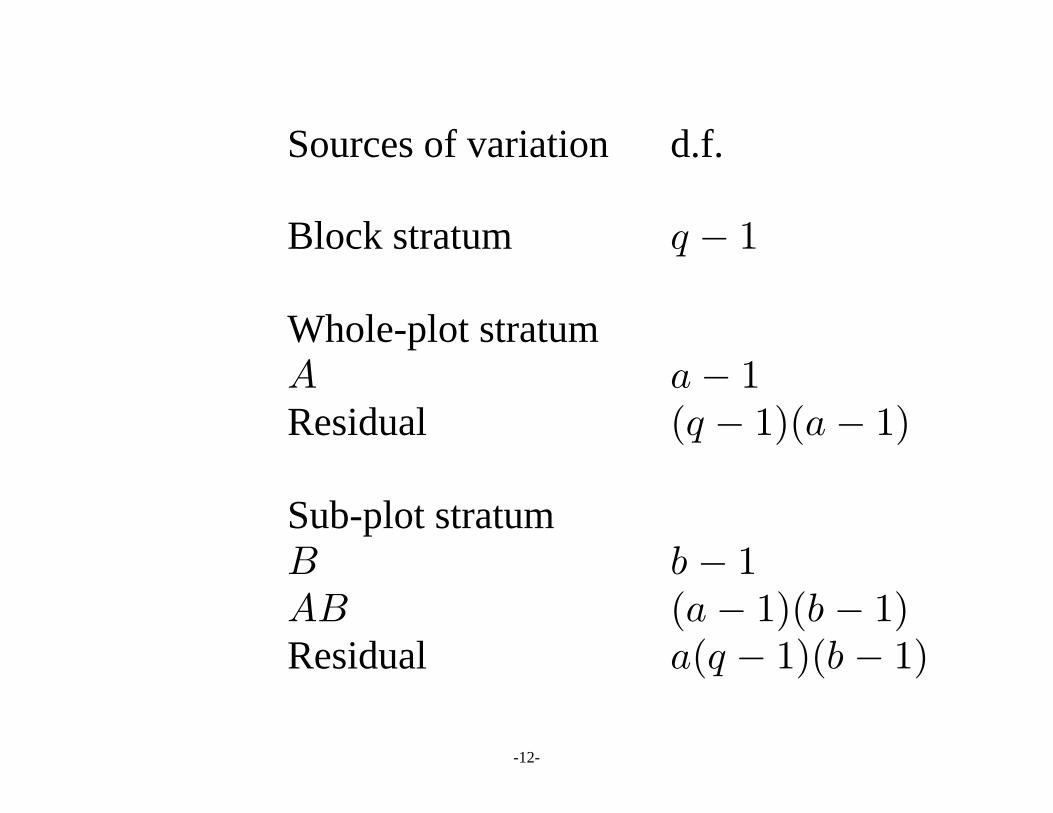
Sources of variation d.f.

Block stratum ; " Whole-plot stratum E + " Residual Ð; "ÑÐ+ "Ñ

Sub-plot stratum F , " EF Ð+ "ÑÐ, "Ñ Residual +Ð; "ÑÐ, "Ñ

-13-

Paper manufacture

Factor 1: three pulp preparation methodsFactor 2: four cooking temperatures

Objective: study the effect on the tensile strength ofthe paper

Three replicates of a 4 3 experiment‚

-14-

A batch of pulp is produced by one of the threemethods; then it is divided into 4 samples. Eachsample is cooked at one temperature.

Block 1 Block 2 Block 3Pulp preparation method 1 2 3 1 2 3 1 2 3

Temperature200 30 34 29 28 31 31 31 35 32225 35 41 26 32 36 30 37 40 34250 37 38 33 40 42 32 41 39 39275 36 42 36 41 40 40 40 44 45

-15-

> y=c(30, 34, 29, 28, 31, 31, 31, 35, 32, 35, 41, 26, 32, 36, 30, 37,40, 34,+ 37, 38, 33, 40, 42, 32, 41, 39, 39, 36, 42, 36, 41, 40, 40, 40, 44,45)> block=gl(3,3,36)> pulp=gl(3,1,36)> temp=gl(4,9,36)> plot=pulp> subplot=temp

> out=aov(y~pulp*temp+Error(block/plot/subplot))> summary(out)

-16-

Error: block Df Sum Sq Mean Sq F value Pr(>F)Residuals 2 77.556 38.778

Error: block:plot Df Sum Sq Mean Sq F value Pr(>F)pulp 2 128.389 64.194 7.0781 0.04854 *Residuals 4 36.278 9.069

Error: block:plot:subplot Df Sum Sq Mean Sq F value Pr(>F)temp 3 434.08 144.69 36.4266 7.449e-08 ***pulp:temp 6 75.17 12.53 3.1538 0.02711 *Residuals 18 71.50 3.97

Nelder (1965a,b) The analysis of randomized experiments withorthogonal block structure. I and II, Proceedings of the RoyalSociety of London, Ser. A, , 147-162 and 163-178.283

Bailey (1981) A unified approach to design of experiments,Journal of Royal Statistical Society Ser. A, , , 214-223.144

Although Nelder (1965a,b) gave a unified treatment of what hecalled 'simple block structures' over ten years ago, his ideas do notseem to have gained wide acceptance. It is a pity, because they areuseful and, I believe, simplifying. However, there seems to be awidespread belief that his ideas are too difficult to be understoodor used by practical statisticians or students.

-17-

From the archive of S-news email list:

"I'm having trouble with what I'm sure is a verysimple problem, i.e., specifying the correctsyntax for a simple split plot design. To checkmy understanding I'm using the cake data setfrom Table 7.5 of Cochran & Cox. .....I can't figure out what error term I need tospecify ....."

-18-

"Speaking as an absolutely committed devotee ofSplus, I think that the Splus syntax for analyzingexperimental designs containing random effectsabsolutely SUCKS!!! … .. I am firmly of theopinion that talking about 'split plots' as such iscounter-productive, confusing, and antiquated. The***right*** way to think about such problems issimply to decide which effects are random and whichare fixed. Then think about expected mean squares,and choose the denominator of your F-statistic sothat under H_0 the ratio of the expected mean squaresis 1 … ."

-19-

"It's a cross-Atlantic culture clash. … .. This divide-and-conquer idea of separating the data using linearfunctions with homogeneous error variances, that is,the spectral decomposition of the variance matrix, Ifind immensely simplifying and natural. … .. Thecontrary notion of putting everything together in onebig anova table with interactions between randomand fixed effects standing in for what really are errorterms and pondering which one goes on the bottom ofwhich other is to lose the plot entirely. … … "

---- Bill Venables

-20-

"The great advantage of the western Pacific view ofspecifying an experiment is that the commandsfollow from the design of the experiment. There is noneed to know anything about fixed or random effects,or denominators of F ratios. Experimenters knowwhat their treatments are, and they know how theyrandomised their experiment. That's all they need tospecify the model, and the correct analysis pops outwhether it was a split plot, confounded factorial,Latin square, or whatever. … .."

-21-

Strip-plot designs

Suppose there are two treatment factors both ofwhich require large plots. If has levels and E + Fhas levels, then one replicate of a complete factorial,requires large plots, which may not be practical.+,

Alternative: Divide the experimental area into +horizontal strips and vertical strips. Each level of,factor is assigned to all the plots in one row, andEeach level of is assigned to all the plots in oneFcolumn.

-22-

Suppose there are replicates and randomization is;carried out within each replicate separately.

Block structure: ( blocks) ( rows) ( columns); ÎÒ + ‚ , Ó

This is a more economic way to run the experiment,but the main effects of the two factors areconfounded with the rows and columns, respectively.

-23-

Many industrial experiments are also run in strip-plots to reduce cost. For example, the fabrication ofintegrated circuits involves a sequence of processingstages. In each stage several wafers may be processedtogether and they are all assigned the same level ofsome treatment factors.

A strip-plot design is useful for experiments with twoprocessing stages.

-24-

Let U e V (respectively, and ) be the subspace of all;<- ‚ " vectors such that has constant valuesC Cover all the entries that correspond to the units thatare in the same block (respectively, same row andsame column). Then dim , dim andÐ Ñ œ ; Ð Ñ œ ;<U edim .Ð Ñ œ ;-V

Four strata other than : block stratum withZ U Z‹; ‹ ;Ð+ Ñ1 d.f., row stratum with 1 d.f.,e Ucolumn stratum with 1 d.f. and unitV U‹ ;Ð, Ñstratum with d.f.Ð Ñ ;Ð+ "ÑÐ, "Ñe V ¼

-25-

The main-effect contrasts of are estimated in theErow stratum, the main-effect contrasts of areFestimated in the column stratum, and the interactioncontrasts of and are estimated in the bottomE F(unit) stratum.

All these estimates and the associated sums ofsquares can be computed in a simple manner.

-26-

ANOVA Sources of variation d.f.

Block stratum ; " Row stratum E + " Residual Ð; "ÑÐ+ "Ñ

Column stratum F , " Residual Ð; "ÑÐ, "Ñ

-27-

Unit stratum EF Ð+ "ÑÐ, "Ñ Residual Ð; "ÑÐ+ "ÑÐ, "Ñ

Total <+, "

This analysis can also be extended easily to thecase of more than two factors.

-28-

An example

Miller ( , vol.39, 153-161, 1997)Technometricsdescribed an experiment for investigating methods ofreducing the wrinkling of clothes being laundered.The experiment was run in two blocks, and fourwashers and four dryers were used. After clothsamples were washed, they were divided into fourgroups such that each group contained exactly onesample from each washer. Each group was thenassigned to one of the dryers.

-29-

The extent of wrinkling on each sample wasevaluated at the end of the experiment. There wereten two-level treatment factors, six of which wereconfigurations of washers and four wereconfigurations of dryers. These factors must be keptat the same level in each washing or drying cycle,respectively. Here we only consider three washerfactors and two dryer factors so that one completereplicate can be accommodated. We shall return todiscuss this example in full after we have introducedfractional factorial designs.

-30-

Washer factors: , , E F GDryer factors: , .I JBlock structure:Ð# ÑÎÒÐ% Ñ ‚ Ð Ñ blocks rows 4 columns ].

Each of the four combinations of and isI Jassigned to one column (dryer) in each block, butsince there are eight combinations of , and ,E F Gone of their factorial effects must be confounded withblocks. One can choose to confound the three-factorinteraction .EFG

-31-

Each of the four combinations of , and withE F Gnone or two of the three factors at level 1 is assignedto each row (washer) in block 1 and each of the otherfour combinations is assigned to each row (washer)in block 2. This results in the following design(before randomization):

Ð"Ñ / 0 /0 + +/ +0 +/0+, +,/ +,0 +,/0 , ,/ ,0 ,/0+- +-/ +-0 +-/0 - -/ -0 -/0,- ,-/ ,-0 ,-/0 +,- +,-/ +,-0 +,-/0

-32-

Assume that all the three-factor and higher-orderinteractions are negligible.

Sources of variation d.f.

Block stratum 1 Row stratum E " F " G " EF " EG " FG "

-33-

Column stratum I " J " IJ " Residual $

Unit stratum EI " EJ " FI " FJ " GI " GJ " Residual 12 Total $"