1

9. Pre- and Post-Processing

Pre-processing:

– creating geometry

– grid-generation

– governing equations

– boundary conditions

Solving

Post-processing

Pre-processing

Solving:

– discretisation

– solution of equations

Post-processing

2

Pre-processing

Solving

Post-processing:

– analysis

– visualisation

CFD Codes

Commercial Codes:

– STAR-CCM+

– Fluent

– FLOW3D

– PowerFLOW

– COMSOL

Open source:

– OpenFOAM

– CodeSaturne

General portals:

– www.cfd-online.com

The Computational Mesh

3

Mesh Generation

Function:

– to decompose the domain into control volumes

Constraints:

– flow geometry

– capabilities of the solver

Output:

– cell vertices (x, y, z)

– connectivity data

Mesh Arrangements

Node locations (cell centres / vertices)

Staggered / co-located

Cell shapes (tetrahedra / hexahedra / arbitrary polyhedra)

Structured (single- or multi-block) / unstructured

Cartesian / curvilinear (orthogonal / non-orthogonal)

…

Storage Locations

cell-centred cell-vertex

staggered

u p

v

4

Cell Shapes

2-d: triangles, quadrilaterals, …

3-d: tetrahedra, hexahedra, …

tetrahedron hexahedron

Areas and Volumes

Vector areas are needed to compute fluxes:

Volumes are needed to compute amounts and averages:

Auρ

Vρ

AΓ

mass flux:

diffusive flux:

amount in cell:

Face Areas

2121 ssA

Triangles

Quadrilaterals

)()( 241321

241321 rrrrddA

4 points are not necessarily coplanar

Vector area is independent of spanning surface

s1

s2

A

A

A

r3

4r

1r2r

5

Some Vector Calculus (Not Examinable)

),,()(gradzyx

z

f

y

f

x

f zyx

ffdivDivergence:

Gradient:

zyx fff

zyx

kji

ffcurlCurl:

),,(zyx

is both a vector and a differential operator

Integral Theorems

Gauss’ Divergence Theorem:

VV

V Aff dd

Stokes’ Theorem:

AA

sfAf dd

VV

dA

A

dsA

Volumes

V

V Ar d3

1

Integrate over an arbitrary closed volume V:

),,( zyxr

3

z

z

y

y

x

xr

VV

VV d3dr

VV

3d

Ar

Divergence:

Position vector:

Use the divergence theorem:

Volumes

V

V Ar d3

1Arbitrary volume:

General polyhedron: faces

ffV Ar3

1

Hexahedron

faces

ffV Ar31

)( 432141 rrrrr f

32161 sss V

Tetrahedron

s3

1s

2s

6

2-D Case

Treat as cells of unit depth

The “volume” of the cell is then the planar area

Outward “face area” vectors derived from Cartesian projections:

x

y

Δ

ΔΔA

(cell boundary traversed anticlockwise)

V

s

A

y

x0

-x

y0

Cell-Averaged Derivatives

)1

)( ttbbnnsseewwavV

AAAAAA

Vav

VxVx

d1

faces

fxf

av

AVx

1

faces

ffavV

A1

)(

V

avV

Ad1

(

Vx V

Vd)(

1e

V

xV

Ae d1

Hexahedra:

Cartesian cell:

)(1

ΔΔwxwexe

wewe ΑΑVxA

ΑΑ

xx

e

n

w

s

Aw

An

Ae

As

)0,0,(

x

Vare

a A

x

V

xAV

d1

Example

A tetrahedral cell has vertices at A(2, –1, 0), B(0, 1, 0), C(2, 1, 1) and D(0, –1, 1).

(a) Find the outward vector areas of all faces. Check that they sum to zero.

(b) Find the volume of the cell.

(c) If the values of at the centroids of the faces (indicated by their vertices) are

BCD = 5, ACD = 3, ABD = 4, ABC = 2,

find the volume-averaged derivatives

avavav zyx

,,

7

Example

In a 2-dimensional unstructured mesh, one cell has the

form of a pentagon. The coordinates of the vertices are

as shown in the figure, whilst the average values of a

scalar on edges a – e are:

a = –7, b = 8, c = –2, d = 5, e = 0

Find:

(a) the area of the pentagon;

(b) the cell-averaged derivatives avav yx

,

(2,-4)

(5,1)

(1,3)

(-3,0)

(-2,-3)

a

bc

d

e

Example

The figure shows the vertices of a single triangular cell in a 2-d unstructured finite-

volume mesh. The accompanying table shows the pressure p and velocity (u,v) on

the faces marked a,b,c at the end of a steady, incompressible flow simulation.

Find:

(a) the area of the triangle;

(b) the net pressure force (per unit depth) on the cell;

(c) the outward volume flow rate (per unit depth) for all faces;

(d) the missing velocity component uc;

(e) the cell-averaged velocity gradients u/x, u/y, v/x, v/y.

(f) Define, mathematically, the acceleration (material derivative) Du/Dt. If the

velocity at the centre of the cell is u = (16/3,–4), use this and the gradients from

part (e) to calculate the acceleration.

edge p u v

a 3 5 –1

b 5 7 –5

c 2 uc –6

(4,0)

(3,5)

(1,1)

bc

ax, u

y, v

Structured Grids

Control volumes indexed by (i, j, k)

Curvilinear Cartesian

8

Unstructured Grids

Fitting Complex Boundaries − Blocking Out Cells

Implemented by a source-term modification:

A lot of redundant matrix operations for cells inside block

)(,0 erlarge numbsb PP F

PPPFFPP sbaa

0

numberlargea

a

P

FF

P

Fitting Complex Boundaries − Volume-of-Fluid (VOF) Approach

One way of handling free-surface calculations.

For moving surfaces, solve a transport equation for fluid fraction f.

Related technique: level-set method.

f = 0

f = 1

f = 0

0 < f < 1

9

Fitting Complex Boundaries − Curvilinear (Body-Fitted) Grids

Curvilinear Grids

sourcediffusionadvectionamountt faces

)()(d

d

Diffusion:

– also requires derivatives parallel to cell faces

Advection:

– all velocity components contribute to mass flux

AAn PE

PE

ΔΓΓ

P

E = const.

=const.

u

v

Fitting Complex Boundaries − Multi-Block Grids

Multiple structured blocks

Grid lines may or may not match at block boundaries

Arbitrary interfaces allow non-coincident grid vertices

Sliding grids used for rotating machinery (pumps; turbines)

2 3 4

51

2 3 4

587

61

6 85321

47

10

Fitting Complex Boundaries − Overset (Chimera) Grids

Disposition of Grid Cells

Local refinement needed where gradients are large:

– solid boundaries

– shear layers

– separation, reattachment and impingement points

– discontinuities (shocks, hydraulic jumps)

Grid-dependence tests necessary

Turbulent calculations impose constraints:

– low-Re calculations: y+ < 1 (ideally)

– wall-function calculations: 30 < y + < 150 (ideally)

Multiple Levels of Grid

Used to confirm grid independence

Exploited by multi-grid methods

Permit estimation of error (and solution improvement)

by Richardson extrapolation

11

Richardson Extrapolation

nΔerror

12

2* Δ2Δ

n

n

n

n

C

C

)Δ2(*

Δ*

Δ2

Δ

Order n

Improved solution by weighted

average from two meshes

12Δ ΔΔ2

n

nC Estimate of error from difference

between solutions on two meshes

Example

A numerical scheme known to be second-order accurate is used to

calculate a steady-state solution on two regular Cartesian meshes A

and B, where the finer mesh A has half the grid spacing of mesh B. The

values of the solution at a particular point are found to be 0.74 using

mesh A and 0.78 using mesh B. Use Richardson extrapolation to:

(a) estimate an improved value of the solution at this point;

(b) estimate the error at this point using the mesh-A solution.

Lewis Fry Richardson Father of modern weather forecasting

12

Summary of Grids

Dictated by:

– flow geometry

– solver capabilities

Grid generator provides vertex and connectivity data

Vector geometry to find areas, volumes and cell-averages

Structured/unstructured meshes

Complex geometries via:

– blocked-out cells

– volume-of-fluid methods

– curvilinear (body-fitted) meshes

– multiblock grids

– overset meshes

Cell density higher in rapidly-varying regions

Boundary Conditions

Boundary Conditions

Inlet:

– velocity inlet

– stagnation / reservoir inlet

Outlet:

– standard outlet

– pressure boundary

– radiation boundary

Wall:

– non-slip (rough/smooth; moving/stationary; adiabatic/heat-transfer)

– slip (inviscid case)

Symmetry plane

Periodic boundary

Free surface

13

Flow Visualisation

Uses of Flow Visualisation

Understanding flow behaviour

Locating important regions

Summarising data

Optimising design

Finding reasons for non-convergence

Publicity

Types of Plot

x-y line graphs

Contour plots

Vector plots

Streamline plots

Mesh plots

Composite plots

14

x-y Graphs

x-y Graphs − Assessment

• Simple

• Widely-available software

• Precise and quantitative

• Direct comparison with experimental data

• Linear or logarithmic scales

• Limited view of flow field

Contour Plots

15

Contour Plots − Assessment

Isoline (2D) or isosurface (3D)

Optional smooth or discrete colour shading

Global view of the flow

Geometric spacing of lines indicates gradient

Not as quantitative as line graphs

Miss detail in small, but important, flow regions

Vector Plots

Vector Plots − Assessment

Direction and magnitude

Used to plot vector quantities (velocity and stress)

May be coloured to indicate magnitude

Excellent first indication of flow behaviour

Interpolation often necessary for non-uniform grids

Not good in flows with wide range of magnitudes

Miss important detail in small regions

Orientation effects deceptive in 3d

16

Streamline Plots

Calculating Streamlines

3D: integrate a particle path ux

td

d

xv

yu

ψ,

ψ

fluxvolumexvyu ddψd

2D: contour the stream function

1

2

volume flux

1

2

dy

dx-v

u

(a) Two adjacent cells in a 2-dimensional Cartesian mesh are shown below, along

with the cell dimensions and some of the velocity components (in m s–1) normal

to cell faces. The value of the stream function at the bottom left corner is

A = 0. Find the value of the stream function at the other vertices B to F. (You

may use either sign convention for the stream function.)

(b) Sketch the pattern of streamlines across the two cells in part (a).

Example

A

D F

C

0.3 m 0.2 m

0.1 m

E

B

5

2

12 3

17

Mesh Plots

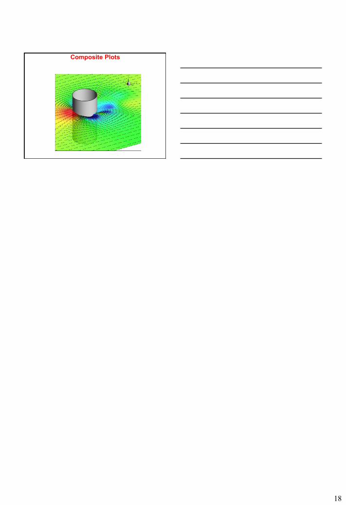
Composite Plots

Composite Plots

18

Composite Plots