10 November 2005. Eric Rasmusen, Erasmuse@indiana.edu. Http://www.rasmusen.org.

9 Adverse Selection

9.1 Introduction: Production Game VI

In Chapter 7, games of asymmetric information were divided between games with moralhazard, in which agents are identical, and games with adverse selection, in which agentsdiffer. In moral hazard with hidden knowledge and adverse selection, the principal tries tosort out agents of different types. In moral hazard with hidden knowledge, the emphasisis on the agent’s action rather than his choice of contract because agents accept contractsbefore acquiring information. Under adverse selection, the agent has private informationabout his type or the state of the world before he agrees to a contract, which means thatthe emphasis is on which contract he will accept.

For comparison with moral hazard, let us consider still another version of the Produc-tion Game of Chapters 7 and 8.

Production Game VI: Adverse Selection

PlayersThe principal and the agent.

The Order of Play

(0) Nature chooses the agent’s ability a, observed by the agent but not by the principal,according to distribution F (a).

(1) The principal offers the agent one or more wage contracts w1(q), w2(q), . . .

(2) The agent accepts one contract or rejects them all.

(3) Nature chooses a value for the state of the world, θ, according to distribution G(θ).Output is then q = q(a, θ).

PayoffsIf the agent rejects all contracts, then πagent = U(a), which might or might not vary withhis type, a; and πprincipal = 0.Otherwise, πagent = U(w, a) and πprincipal = V (q − w).

Under adverse selection, it is not the worker’s effort, but his ability, that is noncon-tractible. Without uncertainty (move (3)), the principal would provide a single contractspecifying high wages for high output and low wages for low output, but either high or lowoutput might be observed in equilibrium, unlike under moral hazard– if both types of agentaccepted the contract. Also, under adverse selection, unlike moral hazard, offering multiple

261

contracts can be an improvement over offering a single contract. The principal might, forexample, provide a flat-wage contract for low-ability agents and an incentive contract forhigh-ability agents.

Production Game VIa puts specific functional forms into the game to illustrate howto find an equilibrium.

Production Game VIa: Adverse Selection with Particular Parameters

PlayersThe principal and the agent.

The Order of Play

(0) Nature chooses the agent’s ability a, unobserved by the principal, according to dis-tribution F (a), which puts probability 0.9 on low ability, a = 0, and probability 0.1on high ability, a = 10.

(1) The principal offers the agent one or more wage contractsW1 = (w1(q = 0), w1(q = 10)), W2 = (w2(q = 0), w2(q = 10)) . . .

(2) The agent accepts one contract or rejects them all.

(3) Nature chooses a value for the state of the world, θ, according to distribution G(θ),which puts equal weight on 0 and 10. Output is then q = Min(a + θ, 10).

PayoffsIf the agent rejects all contracts, then depending on his type his reservation payoff is eitherULow = 3 or UHigh = 2 and the principal’s payoff is πprincipal = 0.Otherwise, Uagent = w and Vprincipal = q − w.

Thus, in Production Game VIa, output is 0 or 10 for the low-ability type of agent,depending on the state of the world, but always 10 for the high-ability agent. The agenttypes also differ in their reservation payoffs: the low- ability agent would work for anexpected wage of 3, but the high-ability agents would require just 2. More realistically thehigh-ability agent would have a higher reservation wage (his ability might be recognizeablein some alternative job), but I have chosen UHigh = 2 to illustrate an interesting feature ofthe equilibrium.

A separating equilibrium isPrincipal: Offer W1 = {w1(q = 0) = 3, w1(q = 10) = 3},

W2 = {w2(q = 0) = 0, w2(q = 10) = 3}

Low agent: Accept W1

High agent: Accept W2

As usual, this is a weak equilibrium. Both Low and High agents are indifferent aboutwhether they accept or reject their contract. The equilibrium indifference of the agents

262

arises from the open-set problem; if the principal were to specify a wage of 3.01 for W2, forexample, the high- ability agent would no longer be indifferent about accepting it insteadof W1.

Let us go through how I came up with the equilibrium contracts above. First, whataction does the principal desire from each type of agent? The agents do not choose effort,but they do choose whether or not to work for the principal, and which contract to accept.The low-ability agent’s expected output is 0.5(0) + 0.5(10)= 5, compared to a reservationpayoff of 3, so the principal will want to hire the low-ability agent if he can do it at anexpected wage of 5 or less. The high-ability agent’s expected output is 0.5(10) + 0.5(10)=10, compared to a reservation payoff of 2, so the principal will want to hire the high-abilityagent if he can do it at an expected wage of 10 or less.

In hidden-action models, the principal tries to construct a contract which will inducethe agent to take the single appropriate action. In hidden-knowledge models, the principaltries to make different actions attractive to different types of agent, so the agent’s choicedepends on the hidden information. The principal’s problem, as Production Game V withits moral hazard and hidden actions, is to maximize his profit subject to

(1) Incentive compatibility (the agent picks the desired contract and actions).

(2) Participation (the agent prefers the contract to his reservation utility).

In a model with hidden knowledge, the incentive compatibility constraint is custom-arily called the self-selection constraint, because it induces the different types of agentsto pick different contracts. A big difference from moral hazard is that in a separating equi-librium there will be an entire set of self-selection constraints, one for each type of agent,since the appropriate contract depends on the hidden information. A second big differenceis that the incentive compatibility constraint could vanish, instead of multiplying. Theprincipal might decide to give up on separating the types of agent, in which case all he hasto do is make sure they all participate.

Here, the participation constraints are, if let πi(Wj) denote the expected payoff an agentof type i gets from contract j,

πL(W1) ≥ ULow; 0.5w1(0) + 0.5w1(10) ≥ 3

πH(W2) ≥ UHigh; 0.5w2(10) + 0.5w2(10) ≥ 2.(1)

Clearly the contracts in our conjectured equilibrium, W1 = (3, 3) and W2 = (0, 3),satisfy the participation constraints. In the equilibrium, the low- and the high-outputwages both matter to the low-ability agent, but only the high-output wage matters to thehigh-ability agent. Both agents, however, end up earning a wage of 3 in each state of theworld, the only difference being that contract W2 would be a very risky contract for thelow-ability agent despite being riskless for the high-ability agent. principal would like tomake W1 risk-free, with the same wage in each state of the world.

In our separating equilibrium, the participation constraint is binding for the “bad”type but not for the “good” type, who would accept a wage as low as 2 if nothing better

263

were available. This is typical of adverse selection models (if there are more than two typesit is the participation constraint of the worst type that is binding, and no other). Theprincipal makes the bad type’s contract unattractive for two reasons. First, if he pays less,he keeps more. Second, when the bad type’s contract is less attractive, the good type canbe more cheaply lured away to a different contract. The principal allows the good type toearn more than his reservation payoff, on the other hand, because the good type always hasthe option of lying about his type and choosing the bad type’s contract, and the good type,with his greater skill, could earn a positive payoff from the bad type’s contract. Thus, theprincipal can never extract all the gains from trade from the good type unless he gives upon making either of his contracts acceptable to the bad type.

Another typical feature of this equilibrium is that the low-ability agent’s contract notonly drives him down to his participation constraint, but is riskless. An alternative wouldbe to offer the low-ability agent a contract of the form W ′

1 = (wl, wh), where it still satisfiesthe participation constraint because 0.5U(wl) + 0.5U(wh) ≥ 3. That is easy enough to doin Production Game VIa, because the agents are risk neutral, and when U(w) = w, thelow-ability agent would be as happy with W ′

1 = (0, 6) as with W1 = (3, 3). But W ′1 would

create a big problem for self-selection, because the high-ability agent would get an expectedpayoff of 6 from it, since his output is always high. Also, if the agents were risk-averse,the risky contract would have to have a higher expected wage than W1, to make up for therisk, and thus would be more expensive for the principal.

Next, look at the self-selection constraints, which are

πL(W1) ≥ πL(W2); 0.5w1(0) + 0.5w1(10) ≥ 0.5w2(0) + 0.5w2(10)

πH(W2) ≥ πH(W1); 0.5w2(10) + 0.5w2(10) ≥ 0.5w1(10) + 0.5w1(10)(2)

The first inequality in (2) says that the contract W2 has to have a low enough expectedreturn for the low-ability agent to deter him from accepting it. The second inequality saysthat the wage contract W1 must be less attractive than W2 to the high-ability agent. Theconjectured equilibrium contracts W1 = (3, 3) and W2 = (0, 3) do this, as can be seen bysubstituting their values into the constraints:

πL(W1) ≥ πL(W2); 0.5(3) + 0.5(3) ≥ 0.5(0) + 0.5(3)

πH(W2) ≥ πH(W1); 0.5(3) + 0.5(3) ≥ 0.5(3) + 0.5(3)(3)

The self-selection constraint is binding for the good type but not for the bad type.This, too, is typical of adverse selection models. The principal wants the good type toreveal his type by choosing the appropriate to the good type as the bad type’s contract.It does not have to be more attractive though (here notice the open-set problem), so theprincipal will minimize his salary expenditures and choose two contracts equally attractiveto the good type. In so doing, however, the principal will have chosen a contract for thegood type that is strictly worse for the bad type, who cannot achieve so high an output soeasily.

It is to show how the participation constraint does not have to be binding for the goodtype that I assumed UHigh = 2 for Production Game VIa. If I had assumed UHigh = 3,

264

then we would still have W2 = (0, 3), but the fact that the “3” came from the self-selectionconstraint would be obscured. And although it is typical that the good agent’s participationconstraint is nonbinding and his incentive compatibility constraint is not, it is by no meansnecessary. If I had assumed UHigh = 4, then we would need W2 = (0, 4) to satisfy theparticipation constraint as cheaply as possible, so it would be binding, and then the self-selection constraint would not be binding. Despite all this, modellers most often expect tofind the bad type’s participation constraint and the good type’s self-selection constraintswill be the binding ones in a two-type model, and the worst agent’s participation constraintand all other agents’ self-selection constraints in a multi-type model.

Once the self-selection and participation constraints are satisfied, weakly or strictly,the agents will not deviate from their equilibrium actions. All that remains to check iswhether the principal could increase his payoff. He cannot, because he makes a profit fromeither contract, and having driven the low- ability agent down to his reservation payoff andthe high-ability agent down to the minimum payoff needed to achieve separation, he cannotfurther reduce their pay.

Competition and Pooling

As with hidden actions, if principals compete in offering contracts under hidden infor-mation, a competition constraint would be added: the equilibrium contract must be asattractive as possible to the agent, since otherwise another principal could profitably lurehim away. An equilibrium may also need to satisfy a part of the competition constraint notfound in hidden actions models: either a nonpooling constraint or a nonseparatingconstraint. If one of several competing principals wishes to construct a pair of separatingcontracts C1 and C2, he must construct it so that not only do agents choose C1 and C2

depending on the state of the world (to satisfy incentive compatibility), but also they prefer(C1, C2) to a pooling contract C3 (to satisfy nonpooling). We only have one principal inProduction Game VI, though, so competition constraints are irrelevant.

Although it is true, however, that the participation constraints must be satisfied foragents who accept the contracts, it is not always the case that they accept different contractsin equilibrium, and if they do not, they do not need to satisfy self-selection constraints.

If all types of agents choose the same strategy in all states, the equilibrium is pooling.Otherwise, it is separating.

The distinction between pooling and separating is different from the distinction be-tween equilibrium concepts. A model might have multiple Nash equilibria, some poolingand some separating. Moreover, a single equilibrium— even a pooling one— can includeseveral contracts, but if it is pooling the agent always uses the same strategy, regardless oftype. If the agent’s equilibrium strategy is mixed, the equilibrium is pooling if the agentalways picks the same mixed strategy, even though the messages and efforts would differacross realizations of the game.

These two terms came up in Section 6.2 in the game of PhD Admissions. Neither typeof student applied in the pooling equilibrium, but one type did in the separating equilibrium.In a principal-agent model, the principal tries to design the contract to achieve separationunless the incentives turn out to be too costly. In Production Game VI, the equilibrium

265

was separating, since the two types of agents choose different contracts.

A separating contract need not be fully separating. If agents who observe a state vari-able θ ≤ 4 accept contract C1 but other agents accept C2, then the equilibrium is separatingbut it does not separate out every type. We say that the equilibrium is fully revealingif the agent’s choice of contract always conveys his private information to the principal.Between pooling and fully revealing equilibria are the imperfectly separating equilibriasynonymously called semi-separating, partially separating, partially revealing, orpartially pooling equilibria.

The possibility of a pooling equilibrium reveals one more step we need to take toestablish that the proposed separating equilibrium in Production Game VIa is really anequilibrium: would the principal do better by offering a pooling contract instead, or aseparating contract under which one type of agent does not participate? All of my derivationabove was to show that the agents would not deviate from the proposed equilibrium, butit might still be that the principal would deviate.

First, would the principal prefer pooling? Then all that is necessary is that the contractas cheaply as possible induce both types of agent to participate. Here, that would requirethat we make the contract barely acceptable to the type with the lowest ability and highestreservation payoff, the low-ability agent. The contract (3, 3) offered by itself would do that,but it would not increase profits over W1 and W2 in our equilibirum above. Either pooling orseparating would yield profits of 0.9(0.5(0−3)+0.5(10−3))+0.1(0.5(10−3)+0.5(10−3)) =2.5.

Second, would the principal prefer a separating contract that “gave up” on one typeof agent? The principal would not want to drive away the high-ability agent, of course,though he could do so by offering a high wage for q = 0 and a low wage for q = 10, becausethe high-ability agent has both greater output and a lower reservation payoff (if we hadUHigh = 11 then the outcome would be different). But if the principal did not have tooffer a contract that gave the low-ability agent his reservation payoff of 3, he could bemore stingy towards the high-ability agent. If there were no low-ability agent, the principalwould offer a contract such as (0, 2) to the high-ability agent, driving him down to hisreservation payoff and increasing the profits from hiring him. Here, however, there are notenough high-ability agents for that to be a good strategy for the principal. His payoff woulddecline to 0.9(0) + 0.1(0.5(10 − 2) + 0.5(10 − 2)) = 0.8, a big decline from 2.5. If 99% ofthe agents were high-ability, instead of 10%, things would have turned out differently, butthere are too many agents who have low ability yet can be efficiently hired for the principalto give up on them.

The Production Game is one setting for adverse selection, and is a good foundationfor modelling it, but the best-known setting, and one which well illustrates the power ofthe idea in explaining everyday phenomenon, is in the used-car market. We will look atthat market in the next few sections. All adverse selection games are games of incompleteinformation, but they might or might not contain uncertainty, moves by Nature occuringafter the agents take their first actions. We will continue using games of certainty inSections 9.2 and 9.3 and wait to look at the effect of uncertainty in Section 9.4. The firstgame will model a used car market in which the quality of the car is known to the seller but

266

not the buyer, and the various versions of the game will differ in the types and numbersof the buyers and sellers. Section 9.4 will return to models with uncertainty, in a modelof adverse selection in insurance. One result there will be that a Nash equilibrium in purestrategies fails to exist for certain parameter values. Section 9.5 applies the idea of adverseselection to explain the magnitude of the bid-ask spread in financial markets, and Section9.6 touches on a variety of other applications.

9.2 Adverse Selection under Certainty: Lemons I and II

Akerlof stimulated an entire field of research with his 1970 model of the market for shoddyused cars (“lemons”), in which adverse selection arises because car quality is better knownto the seller than to the buyer. In agency terms, the principal contracts to buy from theagent a car whose quality, which might be high or low, is noncontractible despite the lackof uncertainty.

We will spend considerable time adding twists to a model of the market in used cars.The game will have one buyer and one seller, but this will simulate competition betweenbuyers, as discussed in Section 7.2, because the seller moves first. If the model had symmet-ric information there would be no consumer surplus. It will often be convenient to discussthe game as if it had many sellers, interpreting one seller whom Nature randomly assignsa type to be a population of sellers of different types, one of whom is drawn by Nature toparticipate in the game.

The Basic Lemons Model

PlayersA buyer and a seller.

The Order of Play

(0) Nature chooses quality type θ for the seller according to the distribution F (θ).The seller knows θ, but while the buyer knows F , he does not know the θ of theparticular seller he faces.

(1) The buyer offers a price P .

(2) The seller accepts or rejects.

PayoffsIf the buyer rejects the offer, both players receive payoffs of zero.Otherwise, πbuyer = V (θ)− P and πseller = P −U(θ), where V and U will be defined later.

The payoffs of both players are normalized to zero if no transaction takes place. (Anormalization is part of the notation of the model rather than a substantive assumption.)The model assigns the players’ utility a base value of zero when no transaction takes place,and the payoff functions show changes from that base. The seller, for instance, gains P ifthe sale takes place but loses U(θ) from giving up the car.

267

The functions F (θ), U(θ), and V (θ) will be specified differently in different versionsof the game. We start with identical tastes and two types (Lemons I ), and generalize to acontinuum of types (Lemons II ). Section 9.3 specifies first that the sellers are identical andvalue cars more than buyers (Lemons III), next that the sellers have heterogeneous tastes(Lemons IV). We will look less formally at other modifications involving risk aversion andthe relative numbers of buyers and sellers.

Lemons I: Identical Tastes, Two Types of Sellers

Let good cars have quality 6, 000 and bad cars (lemons) quality 2, 000, so θ ∈ {2, 000, 6, 000},and suppose that half the cars in the world are of the first type and the other half of thesecond type. A payoff profile of (0,0) will represent the status quo, in which the buyer has$50,000 and the seller has the car. Assume that both players are risk neutral and theyvalue quality at one dollar per unit, so after a trade the payoffs are πbuyer = θ − P andπseller = P − θ. Figure 1 shows the extensive form.

Figure 1: An Extensive Form for Lemons I

If he could observe quality at the time of his purchase, the buyer would be willing toaccept a contract to pay $6,000 for a good car and $2,000 for a lemon. He cannot observequality, however, and we assume that he cannot enforce a contract based on his discoveryonce the purchase is made. Given these restrictions, if the seller offers $4,000, a price equalto the average quality, the buyer will deduce that the car is a lemon. The very fact that thecar is for sale demonstrates its low quality. Knowing that for $4,000 he would be sold onlylemons, the buyer would refuse to pay more than $2,000. Let us assume that an indifferentseller sells his car, in which case half of the cars are traded in equilibrium, all of themlemons.

A friendly advisor might suggest to the owner of a good car that he wait until all thelemons have been sold and then sell his own car, since everyone knows that only good cars

268

have remained unsold. But allowing for such behavior changes the model by adding a newaction. If it were anticipated, the owners of lemons would also hold back and wait for theprice to rise. Such a game could be formally analyzed as a war of attrition (Section 3.2).

The outcome that half the cars are held off the market is interesting, though notstartling, since half the cars do have genuinely higher quality. It is a formalization ofGroucho Marx’s wisecrack that he would refuse to join any club that would accept him asa member. Lemons II will have a more dramatic outcome.

Lemons II: Identical Tastes, a Continuum of Types of Sellers

One might wonder whether the outcome of Lemons I was an artifact of the assumptionof just two types. Lemons II generalizes the game by allowing the seller to be any ofa continuum of types. We will assume that the quality types are uniformly distributedbetween 2, 000 and 6, 000. The average quality is θ = 4, 000, which is therefore the pricethe buyer would be willing to pay for a car of unknown quality if all cars were on themarket. The probability density is zero except on the support [2,000, 6,000], where it isf(θ) = 1/(6, 000− 2, 000), and the cumulative density is

F (θ) =∫ θ

2,000f(x)dx

=∫ θ

2,0001

4000dx =

∣∣∣∣θx=2000

x4000

= θ4000

− 0.5

(4)

The payoff functions are the same as in Lemons I.

The equilibrium price must be less than $4,000 in Lemons II because, as in LemonsI, not all cars are put on the market at that price. Owners are willing to sell only if thequality of their cars is less than 4,000, so while the average quality of all used cars is 4,000,the average quality offered for sale is 3,000. The price cannot be $4,000 when the averagequality is 3,000, so the price must drop at least to $3,000.

If that happens, the owners of cars with values from 3,000 to 4,000 pull their cars offthe market and the average of those remaining is 2,500. The acceptable price falls to $2,500,and the unravelling continues until the price reaches its equilibrium level of $2,000. But atP = 2, 000 the number of cars on the market is infinitesimal. The market has completelycollapsed!

Figure 2 puts the price of used cars on one axis and the average quality of cars offeredfor sale on the other. Each price leads to a different average quality, θ(P ), and the slope ofθ(P ) is greater than one because average quality does not rise proportionately with price. Ifthe price rises, the quality of the marginal car offered for sale equals the new price, but thequality of the average car offered for sale is much lower. In equilibrium, the average qualitymust equal the price, so the equilibrium lies on the 45◦ line through the origin. That lineis a demand schedule of sorts, just as θ(P ) is a supply schedule. The only intersection isthe point (2,000, 2,000).

269

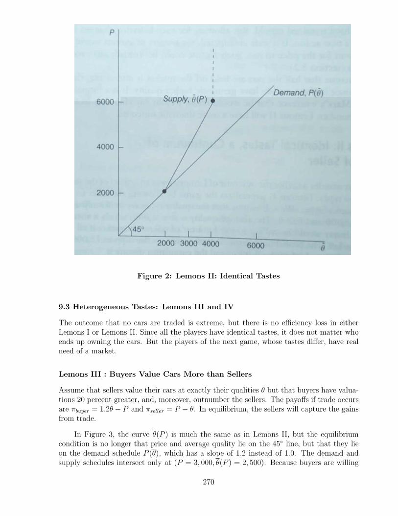
Figure 2: Lemons II: Identical Tastes

9.3 Heterogeneous Tastes: Lemons III and IV

The outcome that no cars are traded is extreme, but there is no efficiency loss in eitherLemons I or Lemons II. Since all the players have identical tastes, it does not matter whoends up owning the cars. But the players of the next game, whose tastes differ, have realneed of a market.

Lemons III : Buyers Value Cars More than Sellers

Assume that sellers value their cars at exactly their qualities θ but that buyers have valua-tions 20 percent greater, and, moreover, outnumber the sellers. The payoffs if trade occursare πbuyer = 1.2θ − P and πseller = P − θ. In equilibrium, the sellers will capture the gainsfrom trade.

In Figure 3, the curve θ(P ) is much the same as in Lemons II, but the equilibriumcondition is no longer that price and average quality lie on the 45◦ line, but that they lieon the demand schedule P (θ), which has a slope of 1.2 instead of 1.0. The demand andsupply schedules intersect only at (P = 3, 000, θ(P ) = 2, 500). Because buyers are willing

270

to pay a premium, we only see partial adverse selection; the equilibrium is partiallypooling. The outcome is inefficient, because in a world of perfect information all the carswould be owned by the “buyers,” who value them more, but under adverse selection theyonly end up owning the low-quality cars.

Figure 3: Buyers Value Cars More than Sellers: Lemons III

Lemons IV: Sellers’ Valuations Differ

In Lemons IV, we dig a little deeper to explain why trade occurs, and we model sellers asconsumers whose valuations of quality have changed since they bought their cars. For aparticular seller, the valuation of one unit of quality is 1+ε, where the random disturbanceε can be either positive or negative and has an expected value of zero. The disturbancecould arise because of the seller’s mistake— he did not realize how much he would enjoydriving when he bought the car— or because conditions changed— he switched to a jobcloser to home. Payoffs if a trade occurs are πbuyer = θ − P and πseller = P − (1 + ε)θ.

If ε = −0.15 and θ = 2, 000 for a particular seller, then $1,700 is the lowest price atwhich he would resell his car. The average quality of cars offered for sale at price P is theexpected quality of cars valued by their owners at less than P , i.e.,

θ(P ) = E (θ | (1 + ε)θ ≤ P ) . (5)

271

Suppose that a large number of new buyers, greater in number than the sellers, appear inthe market, and let their valuation of one unit of quality be $1. The demand schedule,shown in Figure 4, is the 45◦ line through the origin. Figure 4 shows one possible shapefor the supply schedule θ(P ), although to specify it precisely we would have to specify thedistribution of the disturbances.

Figure 4: Lemons IV: Sellers’ Valuations Differ

In contrast to Lemons I, II, and III, here if P ≥ $6, 000 some car owners wouldbe reluctant to sell, because they received positive disturbances to their valuations. Theaverage quality of cars on the market is less than 4,000 even at P = $6, 000. On the otherhand, even if P = $2, 000 some sellers with low-quality cars and negative realizations of thedisturbance do sell, so the average quality remains above 2,000. Under some distributionsof ε, a few sellers hate their cars so much they would pay to have them taken away.

The equilibrium drawn in Figure 4 is (P = $2, 600, θ = 2, 600). Some used cars aresold, but the number is inefficiently low. Some of the sellers have high-quality cars butnegative disturbances, and although they would like to sell their cars to someone whovalues them more, they will not sell at a price of $2,600.

A theme running through all four Lemons models is that when quality is unknown tothe buyer, less trade occurs. Lemons I and II show how trade diminishes, while Lemons III

272

and IV show that the disappearance can be inefficient because some sellers value cars lessthan some buyers. Next we will use Lemons III, the simplest model with gains from trade,to look at various markets with more sellers than buyers, excess supply, and risk-aversebuyers.

More Sellers than Buyers

In analyzing Lemons III we assumed that buyers outnumbered sellers. As a result, thesellers earned producer surplus. In the original equilibrium, all the sellers with quality lessthan 3, 000 offered a price of $3,000 and earned a surplus of up to $1,000. There weremore buyers than sellers, so every seller who wished to sell was able to do so, but the priceequalled the buyers’ expected utility, so no buyer who failed to purchase was dissatisfied.The market cleared.

If, instead, sellers outnumber buyers, what price should a seller offer? At $3,000, notall would-be sellers can find buyers. A seller who proposed a lower price would find willingbuyers despite the somewhat lower expected quality. The buyer’s tradeoff between lowerprice and lower quality is shown in Figure 3, in which the expected consumer surplus isthe vertical distance between the price (the height of the supply schedule) and the demandschedule. When the price is $3,000 and the average quality is 2,500, the buyer expects aconsumer surplus of zero, which is $3, 000 − $1.2 · 2, 500. The combination of price andquality that buyers like best is ($2,000, 2,000), because if there were enough sellers withquality θ = 2, 000 to satisfy the demand, each buyer would pay P = $2, 000 for a car worth$2,400 to him, acquiring a surplus of $400. If there were fewer sellers, the equilibrium pricewould be higher and some sellers would receive producer surplus.

Heterogeneous Buyers: Excess Supply

If buyers have different valuations for quality, the market might not clear, as Charles Wilson(1980) points out. Assume that the number of buyers willing to pay $1.2 per unit of qualityexceeds the number of sellers, but that buyer Smith is an eccentric whose demand for highquality is unusually strong. He would pay $100,000 for a car of quality 5,000 or greater,and $0 for a car of any lower quality.

In Lemons III without Smith, the outcome is a price of $3,000, an average marketquality of 2,500, and a market quality range between 2,000 and 3,000. Smith would beunhappy with this, since he has zero probability of finding a car he likes. In fact, he wouldbe willing to accept a price of $6,000, so that all the cars, from quality 2,000 to 6,000, wouldbe offered for sale and the probability that he buys a satisfactory car would rise from 0 to0.25. But Smith would not want to buy all the cars offered to him, so the equilibrium hastwo prices, $3,000 and $6,000, with excess supply at the higher price.

Strangely enough, Smith’s demand function is upward sloping. At a price of $3,000,he is unwilling to buy; at a price of $6,000, he is willing, because expected quality riseswith price. This does not contradict basic price theory, for the standard assumption ofceteris paribus is violated. As the price increases, the quantity demanded would fall if allelse stayed the same, but all else does not— quality rises.

273

Risk Aversion

We have implicitly assumed, by the choice of payoff functions, that the buyers and sellersare both risk neutral. What happens if they are risk averse— that is, if the marginalutilities of wealth and car quality are diminishing? Again we will use Lemons III and theassumption of many buyers.

On the seller’s side, risk aversion changes nothing. The seller runs no risk becausehe knows exactly the price he receives and the quality he surrenders. But the buyer doesbear risk, because he buys a car of uncertain quality. Although he would pay $3,600 fora car he knows has quality 3,000, if he is risk averse he will not pay that much for a carwith expected quality 3,000 but actual quality of possibly 2,500 or 3,500: he would obtainless utility from adding 500 quality units than from subtracting 500. The buyer would payperhaps $2,900 for a car whose expected quality is 3,000 where the demand schedule isnonlinear, lying everywhere below the demand schedule of the risk- neutral buyer. As aresult, the equilibrium has a lower price and average quality.

9.4 Adverse Selection under Uncertainty: Insurance Game III

The term “adverse selection,” like “moral hazard,” comes from insurance. Insurance paysmore if there is an accident than otherwise, so it benefits accident-prone customers morethan safe ones and a firm’s customers are “adversely selected” to be accident-prone. Theclassic article on adverse selection in insurance markets is Rothschild & Stiglitz (1976),which begins, “Economic theorists traditionally banish discussions of information to foot-notes.” How things have changed! Within ten years, information problems came to domi-nate research in both microeconomics and macroeconomics.

We will follow Rothschild & Stiglitz in using state-space diagrams, and we will use aversion of Section 8.5’s Insurance Game. Under moral hazard, Smith chose whether to beCareful or Careless. Under adverse selection, Smith cannot affect the probability of atheft, which is chosen by Nature. Rather, Smith is either Safe or Unsafe, and while hecannot affect the probability that his car will be stolen, he does know what the probabilityis.

Insurance Game III

PlayersSmith and two insurance companies.

The Order of Play

(0) Nature chooses Smith to be either Safe, with probability 0.6, or Unsafe, with prob-ability 0.4. Smith knows his type, but the insurance companies do not.

(1) Each insurance company offers its own contract (x, y) under which Smith pays pre-mium x unconditionally and receives compensation y if there is a theft.

(2) Smith picks a contract.

274

(3) Nature chooses whether there is a theft, using probability 0.5 if Smith is Safe and0.75 if he is Unsafe.

PayoffsSmith’s payoff depends on his type and the contract (x, y) that he accepts. Let U ′ > 0 andU ′′ < 0.

πSmith(Safe) = 0.5U(12− x) + 0.5U(0 + y − x).

πSmith(Unsafe) = 0.25U(12− x) + 0.75U(0 + y − x).

The companies’ payoffs depend on what types of customers accept their contracts, asshown in Table 1.

Table 1 Insurance Game III Payoffs

Company payoff Types of customers

0 no customers

0.5x + 0.5(x− y) just Safe

0.25x + 0.75(x− y) just Unsafe

0.6[0.5x + 0.5(x− y)] + 0.4[0.25x + 0.75(x− y)] Unsafe and Safe

Smith is Safe with probability 0.6 and Unsafe with probability 0.4. Without insur-ance, Smith’s dollar wealth is 12 if there is no theft and 0 if there is, depicted in Figure 5 ashis endowment in state space, ω = (12, 0). If Smith is Safe, a theft occurs with probability0.5, but if he is Unsafe the probability is 0.75. Smith is risk averse (because U ′′ < 0) andthe insurance companies are risk neutral.

275

Figure 5: Insurance Game III: Nonexistence of a Pooling Equilibrium

If an insurance company knew that Smith was Safe, it could offer him insurance at apremium of 6 with a payout of 12 after a theft, leaving Smith with an allocation of (6, 6).This is the most attractive contract that is not unprofitable, because it fully insures Smith.Whatever the state, his allocation is 6.

Figure 5 shows the indifference curves of Smith and an insurance company, with theno-insurance starting point at ω = (12, 0). A higher insurance premium reduces Smith’swealth in both states of the world; a higher theft insurance payout increases Smith’s wealthin the state of the world in which there is a theft. The insurance company is risk neutral,so its indifference curve is a straight line with negative slope, since to keep the company’s

276

profit constant, the decrease in profit from a rise in Smith’s wealth if there is no theft mustbe balanced by an increase in profit from a fall in Smith’s wealth if there is a theft.

If Smith will be a customer regardless of his type, the company’s indifference curvebased on its expected profits is ωF (although if the company knew that Smith was Safe,the indifference curve would be steeper, and if it knew he was Unsafe, the curve would beless steep). The insurance company is indifferent between ω and C1, at both of which itsexpected profits are zero. Smith is risk averse, so his indifference curves are convex, andclosest to the origin along the 45◦ line if the probability of Theft is 0.5. He has two setsof indifference curves, solid if he is Safe and dotted if he is Unsafe.

Figure 5 shows why no Nash pooling equilibrium exists. To make zero profits, theequilibrium must lie on the line ωF . It is easiest to think about these problems by imaginingan entire population of Smiths, whom we will call “customers.” Pick a contract C1 anywhereon ωF and think about drawing the indifference curves for the Unsafe and Safe customersthat pass through C1. Safe customers are always willing to trade Theft wealth for NoTheft wealth at a higher rate than Unsafe customers. At any point, therefore, the slopeof the solid (Safe) indifference curve is steeper than that of the dashed (Unsafe) curve.Since the slopes of the dashed and solid indifference curves differ, we can insert anothercontract, C2, between them and just barely to the right of ωF . The Safe customers prefercontract C2 to C1, but the Unsafe customers stay with C1, so C2 is profitable— since C2

only attracts Safes, it need not be to the left of ωF to avoid losses. But then the originalcontract C1 was not a Nash equilibrium, and since our argument holds for any poolingcontract, no pooling equilibrium exists.

The attraction of the Safe customers away from pooling is referred to as creamskimming, although profits are still zero when there is competition for the cream. Wenext consider whether a separating equilibrium exists, using Figure 6. The zero-profitcondition requires that the Safe customers take contracts on ωC4 and the Unsafe’s onωC3.

277

Figure 6: A Separating Equilibrium for Insurance Game III

The Unsafes will be completely insured in any equilibrium, albeit at a high price.On the zero-profit line ωC3, the contract they like best is C3, which the Safe’s are nottempted to take. The Safe’s would prefer contract C4, but C4 uniformly dominates C3,so it would attract Unsafes too, and generate losses. To avoid attracting Unsafes, theSafe contract must be below the Unsafe indifference curve. Contract C5 is the fullestinsurance the Safes can get without attracting Unsafes: it satisfies the self-selection andcompetition constraints.

Contract C5, however, might not be an equilibrium either. Figure 7 is the same asFigure 6 with a few additional points marked. If one firm offered C6, it would attractboth types, Unsafe and Safe, away from C3 and C5, because it is to the right of theindifference curves passing through those points. Would C6 be profitable? That dependson the proportions of the different types. The assumption on which the equilibrium ofFigure 6 is based is that the proportion of Safe’s is 0.6, so the zero-profit line for poolingcontracts is ωF and C6 would be unprofitable. In Figure 7 it is assumed that the proportionof Safes is higher, so the zero-profit line for pooling contracts would be ωF ′ and C6, lying to

278

its left, is profitable. But we already showed that no pooling contract is Nash, so C6 cannotbe an equilibrium. Since neither a separating pair like (C3, C5) nor a pooling contract likeC6 is an equilibrium, no equilibrium whatsoever exists.

Figure 7: Curves for which there Is No Equilibrium in Insurance Game III

The essence of nonexistence here is that if separating contracts are offered, somecompany is willing to offer a superior pooling contract; but if a pooling contract is offered,some company is willing to offer a separating contract that makes it unprofitable. Amonopoly would have a pure-strategy equilibrium, but in a competitive market only amixed-strategy Nash equilibrium exists (see Dasgupta & Maskin [1986b]).

*9.5 Market Microstructure

The prices of securities such as stocks depend on what investors believe is the value of theassets that underly them. The value are highly uncertain, and new information about themis constantly being generated. The market microstructure literature is concerned with hownew information enters the market. In the paradigmatic situation, an informed trader has

279

private information about the asset value that he hopes to use to make profitable trades,but other traders know that someone might have private information. This is adverseselection, because the informed trader has better information on the value of the stock,and no uninformed trader wants to trade with an informed trader– the informed trade isa “bad type” from the point of view of the other side of the market. . An institution thatmany markets have developed is the “marketmaker” or “specialist”, a trader in a particularstock who is always willing to buy or sell to keep the market going. Other traders feel saferin trading with the marketmaker than with a potentially informed trader, but this justtransfers the adverse selection problem to the marketmaker, who always loses when hetrades with someone who is informed.

The two models in this section will look at how a marketmaker deals with the problemof informed trading. Both are descendants of the verbal model in Bagehot (1971).(“Bage-hot”, pronounced “badget”, is a pseudonym for Jack Treynor. See Glosten & Milgrom[1985] for a formalization.) In the Bagehot model, there may or may not be one or moreinformed traders, but the informed traders as a group have a trade of fixed size if they arepresent. The marketmaker must decide how big a bid-ask spread to charge. In the Kylemodel, there is one informed trader, who decides how much to trade. On observing theimbalance of orders, the marketmaker decides what price to offer.

The Bagehot Model

PlayersThe informed trader and two competing marketmakers.

The Order of Play

(0) Nature chooses the asset value v to be either p0 − δ or p0 + δ with equal probability.The marketmakers never observe the asset value, nor do they observe whether anyoneelse observes it, but the “informed” trader observes v with probability θ.

(1) The marketmakers choose their spreads s, offering prices pbid = p0 − s2

at which theywill buy the security and pask = p0 + s

2for which they will sell it.

(2) The informed trader decides whether to buy one unit, sell one unit, or do nothing.

(3 ) Noise traders buy n units and sell n units.

PayoffsEveryone is risk neutral. The informed trader’s payoff is (v − pask) if he buys, (pbid − v) ifhe sells, and zero if he does nothing. The marketmaker who offers the highest pbid tradeswith all the customers who wish to sell, and the marketmaker who offers the lowest pask

trades with all the customers who wish to buy. If the marketmakers set equal prices, theysplit the market evenly. A marketmaker who sells x units gets a payoff of x(pask − v), anda marketmaker who buys x units gets a payoff of x(v − pbid).

280

Optimal strategies are simple. Competition between the marketmakers will make theirprices identical and their profits zero. The informed trader should buy if v > pask and sellif v < pbid. He has no incentive to trade if v ∈ [pbid, pask].

A marketmaker will always lose money trading with the informed trader, but if s > 0,so pask > p0 and pbid < p0, he will earn positive expected profits in trading with the noisetraders. Since a marketmaker could specialize in either sales or purchases, he must earnzero expected profits overall from either type of trade. Centering the bid-ask spread on theexpected value of the stock, p0, ensures this. Marketmaker sales will be at the ask priceof (p0 + s/2). With probability 0.5, this is above the true value of the stock, (p0 − δ), inwhich case the informed trader will not buy but the marketmakers will earn a total profit ofn[(p0+s/2)−(p0−δ)] from the noise traders. With probability 0.5, the ask price of (p0+s/2)is below the true value of the stock, (p0 + δ), in which case the informed trader will beinformed with probability θ and buy one unit and the noise traders will buy n more in anycase, so the marketmakers will earn a total expected profit of (n + θ)[(p0 + s/2)− (p0 + δ)],a negative number. For marketmaker profits from sales at the ask price to be zero overall,this expected profit must be zero:

0.5n[(p0 + s/2)− (p0 − δ)] + 0.5(n + θ)[(p0 + s/2)− (p0 + δ)] = 0 (6)

Equation (6) implies that n[s/2 + δ] + (n + θ)[s/2− δ] = 0, so

s∗ =2δθ

2n + θ. (7)

The profit from marketmaker purchases must similarly equal zero, and will for the samespread s∗, though we will not go through the algebra here.

Equation (7) has a number of implications. First, the spread s∗ is positive. Eventhough marketmakers compete and have zero transactions costs, they charge a differentprice to buy and to sell. They make money dealing with the noise traders but lose moneywith the informed trader, if he is present. The comparative statics reflect this. s∗ rises in δ,the dispersion of the true value, because divergent true values increase losses from tradingwith the informed trader, and s∗ falls in n, which reflects the number of noise tradersrelative to informed traders, because when there are more noise traders, the profits fromtrading with them are greater. The spread s∗ rises in θ, the probability that the informedtrader really has inside information, which is also intuitive but requires a little calculus todemonstrate, using equation (7):

∂s∗

∂θ=

2δ

2n + θ− 2δθ

(2n + θ)2=

(1

(2n + θ)2

)(4δn + 2δθ − 2δθ) > 0. (8)

The second model of market microstructure, important because it is commonly used asa foundation for more complicated models, is the Kyle model. It focuses on the decision ofthe informed trader, not the marketmaker. The Kyle model is set up so that marketmakerobserves the trade volume before he chooses the price.

The Kyle Model (Kyle [1985])

281

PlayersThe informed trader and two competing marketmakers.

The Order of Play

(0) Nature chooses the asset value v from a normal distribution with mean p0 and varianceσ2

v , observed by the informed trader but not by the marketmakers.

(1) The informed trader offers a trade of size x(v), which is a purchase if positive and asale if negative, unobserved by the marketmaker.

(2) Nature chooses a trade of size u by noise traders, unobserved by the marketmaker,where u is distributed normally with mean zero and variance σ2

u.

(3) The marketmakers observe the total market trade offer y = x + u, and choose pricesp(y).

(4) Trades are executed. If y is positive (the market wants to purchase, in net), whichevermarketmaker offers the lowest price executes the trades; if y is negative (the marketwants to sell, in net), whichever marketmaker offers the highest price executes thetrades. The value v is then revealed to everyone.

PayoffsAll players are risk neutral. The informed trader’s payoff is (v − p)x. The marketmaker’spayoff is zero if he does not trade and (p− v)y if he does.

An equilibrium for this game is the strategy profile

x(v) = (v − p0)

(σu

σv

)(9)

and

p(y) = p0 +

(σv

2σu

)y. (10)

This is reasonable. It says that the informed trader will increase the size of his tradeas v gets bigger relative to p0 (and he will sell, not buy, if v−p0 < 0), and the marketmakerwill increase the price he charges if y is bigger and more people want to sell, which is anindicator that the informed trader might be trading heavily. The variances of the assetvalue (σ2

v) and the noise trading (σ2u) enter as one would expect, and they matter only in

their relation to each other. If σ2v

σ2u

is large, then the asset value fluctuates more than theamount of noise trading, and it is difficult for the informed trader to conceal his tradesunder the noise. The informed trader will trade less, and a given amount of trading willcause a greater response from the marketmaker. One might say that the market is less“liquid”: a trade of given size will have a greater impact on the price.

I will not (and cannot) prove uniqueness of the equilibrium, since it is very hard tocheck all possible profiles of nonlinear strategies, but I will show that {(9), (10)} is Nash

282

and is the unique linear equilibrium. To start, hypothesize that the informed trader uses alinear strategy, so

x(v) = α + βv (11)

for some constants α and β. Competition between the marketmakers means that theirexpected profits will be zero, which requires that the price they offer be the expected valueof v. Thus, their equilibrium strategy p(y) will be an unbiased estimate of v given theirdata y, where they know that y is normally distributed and that

y = x + u= α + βv + u.

(12)

This means that their best estimate of v given the data y is, following the usual regressionrule (which readers unfamiliar with statistics must accept on faith),

E(v|y) = E(v) +(

cov(v,y)var(y)

)y

= p0 +(

βσ2v

β2σ2v+σ2

u

)y

= p0 + λy,

(13)

where λ is a new shorthand variable to save writing out the term in parentheses.

The function p(y) will be a linear function of y under our assumption that x is a linearfunction of v. Given that p(y) = p0 + λy, what must next be shown is that x will indeedbe a linear function of v. Start by writing the informed trader’s expected payoff, which is

Eπi = E([v − p(y)]x)

= E([v − p0 − λ(x + u)]x)

= [v − p0 − λ(x + 0)]x,

(14)

since E(u) = 0. Maximizing the expected payoff with respect to x yields the first-ordercondition

v − p0 − 2λx = 0, (15)

which on rearranging becomes

x = − p0

2λ+

(1

2λ

)v. (16)

Equation (16) establishes that x(v) is linear, given that p(y) is linear. All that is left is tofind the value of λ. By comparing (16) and (11) we can see that β = 1

2λ. Substituting this

β into the value of λ from (13) leads to

λ =βσ2

v

β2σ2v + σ2

u

=σ2

v

2λσ2

v

(4λ2)+ σ2

u

, (17)

283

which upon solving for λ yields λ = σv

2σu. Since β = 1

2λ, it follows that β = σu

σv. These values

of λ and β together with equation (16) give the strategies asserted at the start in equations(9) and (10).

The Bagehot model is perhaps a better explanation of why marketmakers might chargea bid/ask spread even under competitive conditions and with zero transactions costs. Itsassumption is that the marketmaker cannot change the price depending on volume, butmust instead offer a price, and then accept whatever order comes along—a buy order, or asell order.

The two main divisions of the field of finance are corporate finance and asset pricing.Corporate finance, the study of such things as project choice, capital structure, and mergershas the most obvious applications of game theory, but the Bagehot and Kyle models showthat the same techniques are also important in asset pricing. For more information, Irecommend Harris & Raviv (1995).

*9.6 A Variety of Applications

Price Dispersion

Usually the best model for explaining price dispersion is a search model— Salop & Stiglitz(1977), for example, which is based on buyers whose search costs differ. But although wepassed over it quickly in Section 9.3, the Lemons model with Smith, the quality-consciousconsumer, generated not only excess supply, but price dispersion as well. Cars of the sameaverage quality were sold for $3,000 and $6,000.

Similarly, while the most obvious explanation for why brands of stereo amplifiers sellat different prices is that customers are willing to pay more for higher quality, adverseselection contributes another explanation. Consumers might be willing to pay high pricesbecause they know that high-priced brands could include both high-quality and low-qualityamplifiers, whereas low- priced brands are invariably low quality. The low-quality amplifierends up selling at two prices: a high price in competition with high-quality amplifiers, and,in different stores or under a different name, a low price aimed at customers less willing totrade dollars for quality.

This explanation does depend on sellers of amplifiers incurring a large enough fixedset-up or operating cost. Otherwise, too many low-quality brands would crowd into themarket, and the proportion of high-quality brands would be too small for consumers tobe willing to pay the high price. The low-quality brands would benefit as a group fromentry restrictions: too many of them spoil the market, not through price competition butthrough degrading the average quality.

Health Insurance

284

Medical insurance is subject to adverse selection because some people are healthier thanothers. The variance in health is particularly high among old people, who sometimes havedifficulty in obtaining insurance at all. Under basic economic theory this is a puzzle: theprice should rise until supply equals demand. The problem is pooling: when the price ofinsurance is appropriate for the average old person, healthier ones stop buying. The pricemust rise to keep profits nonnegative, and the market disappears, just as in Lemons II.

If the facts indeed fit this story, adverse selection is an argument for government-enforced pooling. If all old people are required to purchase government insurance, thenwhile the healthier of them may be worse off, the vast majority could be helped.

Using adverse selection to justify medicare, however, points out how dangerous manyof the models in this book can be. For policy questions, the best default opinion is thatmarkets are efficient. On closer examination, we have found that many markets are ineffi-cient because of strategic behavior or information asymmetry. It is dangerous, however, toimmediately conclude that the government should intervene, because the same argumentsapplied to government show that the cure might be worse than the disease. The analyst ofhealth care needs to take seriously the moral hazard and rent-seeking that arise from gov-ernment insurance. Doctors and hospitals will increase the cost and amount of treatmentif the government pays for it, and the transfer of wealth from young people to the elderly,which is likely to swamp the gains in efficiency, might distort the shape of the governmentprogram from the economist’s ideal.

Henry Ford’s Five-Dollar Day

In 1914 Henry Ford made a much-publicized decision to raise the wage of his auto workersto $5 a day, considerably above the market wage. This pay hike occurred without pressurefrom the workers, who were non-unionized. Why did Ford do it?

The pay hike could be explained by either moral hazard or adverse selection. Inaccordance with the idea of efficiency wages (Section 8.1), Ford might have wanted workerswho worried about losing their premium job at his factory, because they would work harderand refrain from shirking. Adverse selection could also explain the pay hike: by raising hiswage Ford attracted a mixture of low- and high-quality workers, rather than low-qualityalone (see Raff & Summers [1987]).

Bank Loans

Suppose that two people come to you for an unsecured loan of $10,000. One offers to payan interest rate of 10 percent and the other offers 200 percent. Who do you accept? LikeCharles Wilson’s car buyer in Section 9.3 who chose to buy at a high price, you may chooseto lend at a low interest rate.

If a lender raises his interest rate, both his pool of loan applicants and their behaviorchange because adverse selection and moral hazard contribute to a rise in default rates.Borrowers who expect to default are less concerned about the high interest rate thandependable borrowers, so the number of loans shrinks and the default rate rises (see Stiglitz& Weiss [1981]). In addition, some borrowers shift to higher-risk projects with greater

285

chance of default but higher yields when they are successful. In Section 6.6 we wentthrough the model of D. Diamond (1989) which looks at the evolution of this problem asfirms age.

Whether because of moral hazard or adverse selection, asymmetric information canalso result in excess demand for bank loans. The savers who own the bank do not saveenough at the equilibrium interest rate to provide loans to all the borrowers who want loans.Thus, the bank makes a loan to John Smith, while denying one to Joe, his observationallyequivalent twin. Policymakers should carefully consider any laws that rule out arbitraryloan criteria or require banks to treat all customers equally. A bank might wish to restrictits loans to left-handed people, neither from prejudice nor because it is useful to rationloans according to some criterion arbitrary enough to avoid the moral hazard of favoritismby loan officers.

Bernanke (1983) suggests adverse selection in bank loans as an explanation for theGreat Depression in the United States. The difficulty in explaining the Depression is notso much the initial stock market crash as the persistence of the unemployment that followed.Bernanke notes that the crash wiped out local banks and dispersed the expertise of theloan officers. After the loss of this expertise, the remaining banks were less willing to lendbecause of adverse selection, and it was difficult for the economy to recover.

Solutions to Adverse Selection

Even in markets where it apparently does not occur, the threat of adverse selection, likethe threat of moral hazard, can be an important influence on market institutions. Adverseselection can be circumvented in a number of ways besides the contractual solutions wehave been analyzing. I will mention some of them in the context of the used car market.

One set of solutions consists of ways to make car quality contractible. Buyers whofind that their car is defective may have recourse to the legal system if the sellers werefraudulent, although in the United States the courts are too slow and costly to be fullyeffective. Other government bodies such as the Federal Trade Commission may do better byissuing regulations particular to the industry. Even without regulation, private warranties—promises to repair the car if it breaks down— may be easier to enforce than oral claims,by disspelling ambiguity about what level of quality is guaranteed.

Testing (the equivalent of moral hazard’s monitoring) is always used to some extent.The prospective driver tries the car on the road, inspects the body, and otherwise tries toreduce information asymmetry. At a cost, he could even reverse the asymmetry by hiringmechanics who can tell him more about the car than the owner himself knows. The ruleis not always caveat emptor; what should one’s response be to an antique dealer who offersto pay $500 for an apparently worthless old chair?

Reputation can solve adverse selection, just as it can solve moral hazard, but only ifthe transaction is repeated and the other conditions of the models in Chapters 5 and 6 aremet. An almost opposite solution is to show that there are innocent motives for a sale;that the owner of the car has gone bankrupt, for example, and his creditor is selling thecar cheaply to avoid the holding cost.

286

Penalties not strictly economic are also important. One example is the social ostracisminflicted by the friend to whom a lemon has been sold; the seller is no longer invited todinner. Or, the seller might have moral principles that prevent him from defrauding buyers.Such principles, provided they are common knowledge, would help him obtain a higher pricein the used-car market. Akerlof himself has worked on the interaction between social customand markets in his 1980 and 1983 articles. The second of these articles looks directly atthe value of inculcating moral principles, using theoretical examples to show that parentsmight wish to teach their children principles, and that society might wish to give hiringpreference to students from elite schools.

It is by violating the assumptions needed for perfect competition that asymmetricinformation enables government and social institutions to raise efficiency. This points toa major reason for studying asymmetric information: where it is important, noneconomicinterference can be helpful instead of harmful. I find the social solutions particularlyinteresting since, as mentioned earlier in connection with health care, government solutionsintroduce agency problems as severe as the information problems they solve. Noneconomicbehavior is important under adverse selection, in contrast to perfect competition, whichallows an “Invisible Hand” to guide the market to efficiency, regardless of the moral beliefsof the traders. If everyone were honest, the lemons problem would disappear becausethe sellers would truthfully disclose quality. If some fraction of the sellers were honest, butbuyers could not distinguish them from the dishonest sellers, the outcome would presumablybe somewhere between the outcomes of complete honesty and complete dishonesty. Thesubject of market ethics is important, and would profit from investigation by scholarstrained in economic analysis.

9.7 Adverse Selection and Moral Hazard Combined: Production Game VII (newin the 4th edition)

What happens when adverse selection and moral hazard combine, so that agents beginthe game with private information but then also take unobserved actions in the course ofthe game? Production Game VII shows one possibility, in a model that will also be usedat the start of Chapter 10.

Production Game VII: Adverse Selection and Moral Hazard

PlayersThe principal and the agent.

The Order of Play

(0) Nature chooses the state of the world s, observed by the agent but not by the principal,according to distribution F (s), where the state s is Good with probability 0.5 andBad with probability 0.5.

287

(1) The principal offers the agent a wage contract w(q).

(2) The agent accepts or rejects the contract.

(3) The agent chooses effort level e.

(4) Output is q = q(e, s). where q(e, good) = 3e and q(e, bad) = e.

PayoffsIf the agent rejects all contracts, then πagent = U = 0 and πprincipal = 0.Otherwise, πagent = U(e, w, s) = w − e2 and πprincipal = V (q − w) = q − w.

Thus, there is no uncertainty, both principal and agent are risk neutral in money, andeffort is increasingly costly.

In this model, the first-best effort depends on the state of the world. The two socialsurplus maximization problems are

Maximizeeg 3eg − e2

g, (18)

which is solved by the optimal effort eg = 1.5 (and qg = 4.5) in the good state, and

Maximizeeg eb − e2

b , (19)

which is solved by the optimal effort eb = 0.5 (and qb = 0.5)in the bad state.

The problem is that the principal does not know what level of effort and output areappropriate. He does not want to require high output in both states, because if he does, hewill have to pay too high a salary to the agent to compensate for the difficulty of attainingthat output in the bad state. Rather, he must solve the following problem:

Maximizeqg, qb, wg, wb [0.5(qg − wg) + 0.5(qb − wb)], (20)

where the agent has a choice between two forcing contracts, (qg, wg) and (qb, wb), and thecontracts must induce participation and self selection.

The self-selection constraints are based on efforts of e = q/3 for the good state ande = q for the bad state. In the good state, the agent must choose the good-state contract,so

πagent(qg, wg|good) = wg −(qg

3

)2

≥ πagent(qb, wb|good) = wb −(qb

3

)2

(21)

and in the bad state he must choose the bad-state contract,so

πagent(qb, wb|bad) = wb − q2b ≥ πagent(qg, wg|bad) = wg − q2

g . (22)

The participation constraints are

πagent(qg, wg|good) = wg −(qg

3

)2

≥ 0 (23)

288

andπagent(qb, wb|bad) = wb − q2

b ≥ 0. (24)

The bad state’s participation constraint will be binding, since in the bad state theagent will not be tempted by the good-state contract’s higher output and wage. Thus, wecan conclude from constraint (24) that

wb = q2b . (25)

The good state’s participation constraint will not be binding, since there the agentwill be left with an informational rent– the principal must leave the agent some surplus toinduce him to reveal the good state.

The good state’s self-selection constraint will be binding, since in the good state theagent will be tempted to take the easier contract appropriate for the bad state. Thus, wecan conclude from constraint (21) that

wg =(qg

3

)2

+ wb −(qb

3

)2

=(qg

3

)2

+ q2b −

(qb

3

)2

,

(26)

where the second step substitutes for wb from equation (25). The bad state’s self-selectionconstraint will not be binding, since the agent would then not be tempted to produce alarge amount for a large wage.

Now let’s return to the principal’s maximization problem. Having found expressionsfor wb and wg we can rewrite (20) as

Maximizeqg, qb [0.5

(qg −

(qg

3

)2

− q2b +

(qb

3

)2)

+ 0.5(qb − q2b )] (27)

with no constraints. The first-order conditions are

0.5

(1− 2qg

9

)= 0, (28)

so qg = 4.5, and

0.5

(−2qb +

2qb

9

)+ 0.5(1− 2qb) = 0, (29)

so qb ≈ .26. We can then find the wages that satisfy the constraints, which are wg ≈ 2.32and wb ≈ 0.07.

Thus, in the second-best world of information asymmetry, the effort in the good stateremains the first-best effort, but second-best effort in the bad state is lower than first-best. This results from the principal’s need to keep the bad- state contract from beingtoo attractive in the good state. Bad-state output and compensation must be suppressed.Good-state output, on the other hand, should be left at the first-best level, since the agentwill not be tempted by that contract in the bad state.

289

Also, observe that in the good state the agent earns an informational rent. As ex-plained earlier, this is because the good-state agent could always earn a positive payoff bypretending the state was bad and taking that contract, so any contract that separates outthe good-state agent (while leaving some contract acceptable to the bad-state agent) mustalso have a positive payoff.

290

Notes

N9.1 Introduction: Production Game VI

• In moral hazard with hidden knowledge, the contract must ordinarily satisfy only one partic-ipation constraint, whereas in adverse selection problems there is a different participationconstraint for each type of agent. An exception is if there are constraints limiting howmuch an agent can be punished in different states of the world. If, for example, there arebankruptcy constraints, then, if the agent has different wealths across the N possible statesof the world, there will be N constraints for how negative his wage can be, in additionto the single participation constraint. These can be looked at as interim participationconstraints, since they represent the idea that the agent wants to get out of the contractonce he observes the state of the world midway through the game.

• Gresham’s Law (“Bad money drives out good” ) is a statement of adverse selection. Onlydebased money will be circulated if the payer knows the quality of his money better thanthe receiver. The same result occurs if quality is common knowledge, but for legal reasonsthe receiver is obligated to take the money, whatever its quality. An example of the firstis Roman coins with low silver content; and of the second, Zambian currency with anovervalued exchange rate.

• Most adverse selection models have types that could be called “good” and “bad,” becauseone type of agent would like to pool with the other, who would rather be separate. It isalso possible to have a model in which both types would rather separate— types of workerswho prefer night shifts versus those who prefer day shifts, for example— or two types whoboth prefer pooling— male and female college students.

• Two curious features of labor markets is that workers of widely differing outputs seem tobe paid identical wages and that tests are not used more in hiring decisions. Schmidtand Judiesch (as cited in Seligman [1992], p. 145) have found that in jobs requiring onlyunskilled and semi-skilled blue-collar workers, the top 1 percent of workers, as defined byperformance on ability tests not directly related to output, were 50 percent more productivethan the average. In jobs defined as “high complexity” the difference was 127 percent.

At about the same time as Akerlof (1970), another seminal paper appeared on adverseselection, Mirrlees (1971), although the relation only became clear later. Mirrlees looked atoptimal taxation and the problem of how the government chooses a tax schedule given thatit cannot observe the abilities of its citizens to earn income, and this began the literatureon mechanism design. Used cars and income taxes do not appear similar, but in bothsituations an uninformed player must decide how to behave to another player whose typehe does not know. Section 10.4 sets out a descendant of Mirrlees (1971) in a model ofgovernment procurement: much of government policy is motivated by the desire to createincentives for efficiency at minimum cost while eliciting information from individuals withsuperior information.

N9.2 Adverse Selection under Certainty: Lemons I and II

• Suppose that the cars of Lemons II lasted two periods and did not physically depreciate. Anaive economist looking at the market would see new cars selling for $6,000 (twice $3,000)and old cars selling for $2,000 and conclude that the service stream had depreciated by 33percent. Depreciation and adverse selection are hard to untangle using market data.

291

• Lemons II uses a uniform distribution. For a general distribution F , the average qualityθ(P ) of cars with quality P or less is

θ(P ) = E(θ|θ ≤ P ) =

∫ P−∞ xF ′(x)dx

F (P ). (30)

Equation (30) also arises in physics (the equation for the center of gravity) and nonlineareconometrics (the likelihood equation). Think of θ(P ) as a weighted average of the valuesof θ up to P , the weights being densities. Having multiplied by all these weights in thenumerator, we have to divide by their “sum,” F (P ) =

∫ P−∞ F ′(x)dx, in the denominator,

giving rise to equation (30).

N9.3 Heterogeneous Tastes: Lemons III and IV

• You might object to a model in which the buyers of used cars value quality more than thesellers, since the sellers are often richer people. Remember that quality here is “quality ofused cars,” which is different from “quality of cars.” The utility functions could be mademore complicated without abandoning the basic model. We could specify something likeπbuyer = θ + k/θ − P , where θ2 > k. Such a specification implies that the lower is thequality of the car, the greater the difference between the valuations of buyer and seller.

• In the original article, Akerlof (1970), the quality of new cars is uniformly distributedbetween zero and 2, and the model is set up differently, with the demand and supply curvesoffered by different types of traders and net supply and gross supply presented ratherconfusingly. Usually the best way to model a situation in which traders sell some of theirendowment and consume the rest is to use only gross supplies and demands. Each oldowner supplies his car to the market, but in equilibrium he might buy it back, havingbetter information about his car than the other consumers. Otherwise, it is easy to counta given unit of demand twice, once in the demand curve and once in the net supply curve.

• See Stiglitz (1987) for a good survey of the relation between price and quality. Leibenstein(1950) uses diagrams to analyze the implications of individual demand being linked to themarket price of quantity in markets for “bandwagon,” “snob,” and “Veblen” goods.

• Risk aversion is concerned only with variability of outcomes, not their level. If the qualityof used cars ranges from 2,000 to 6,000, buying a used car is risky. If all used cars are ofquality 2,000, buying a used car is riskless, because the buyer knows exactly what he isgetting.

In Insurance Game III in Section 9.4, the separating contract for the Unsafe consumerfully insures him: he bears no risk. But in constructing the equilibrium, we had to be verycareful to keep the Unsafes from being tempted by the risky contract designed for theSafes. Risk is a bad thing, but as with old age, the alternative is worse. If Smith werecertain his car would be stolen, he would bear no risk, because he would be certain to havelow utility.

• To the buyers in Lemons IV, the average quality of cars for a given price is stochasticbecause they do not know which values of ε were realized. To them, the curve θ(P ) is onlythe expectation of the average quality.

292

• Lemons III′: Minimum Quality of Zero. If the minimum quality of car in Lemons IIIwere 0, not 2,000, the resulting game (Lemons III′) would be close to the original Akerlof(1970) specification. As Figure 8 shows, the supply schedule and the demand scheduleintersect at the origin, so that the equilibrium price is zero and no cars are traded. Themarket has shut down entirely because of the unravelling effect described in Lemons II.Even though the buyers are willing to accept a quality lower than the dollar price, theprice that buyers are willing to pay does not rise with quality as fast as the price neededto extract that average quality from the sellers, and a car of minimum quality is valuedexactly the same by buyers and sellers. A 20 percent premium on zero is still zero. Theefficiency implications are even stronger than before, because at the optimum all the oldcars are sold to new buyers, but in equilibrium, none are.

Figure 8: Lemons III′ When Buyers Value Cars More and the MinimumQuality is Zero

N9.4 Adverse Selection under Uncertainty: Insurance Game III

• Markets with two types of customers are very common in insurance, because it is easy todistinguish male from female, both those types are numerous, and the difference betweenthem is important. Males under age 25 pay almost twice the auto insurance premiums offemales, and females pay 10 to 30 percent less for life insurance. The difference goes bothways, however: Aetna charges a 35-year old woman 30 to 50 percent more than a man formedical insurance. One market in which rates do not differ much is disability insurance.Women do make more claims, but the rates are the same because relatively few women buythe product (Wall Street Journal, p. 21, 27 August 1987).

293

N9.6 A Variety of Applications

• Economics professors sometimes make use of self-selection for student exams. One of mycolleagues put the following instructions on an MBA exam, after stating that either Question5 or 6 must be answered.

“The value of Question 5 is less than that of Question 6. Question 5, however, isstraightforward and the average student may expect to answer it correctly. Question 6is more tricky: only those who have understood and absorbed the content of the coursewell will be able to answer it correctly... For a candidate to earn a final course grade ofA or higher, it will be necessary for him to answer Question 6 successfully.”

Making the question even more self-referential, he asked the students for an explanation ofits purpose.

Another of my colleagues tried asking who in his class would be willing to skip the examand settle for an A−. Those students who were willing, received an A−. The others got A’s.But nobody had to take the exam. (This method did upset a few people). More formally,Guasch & Weiss (1980) have looked at adverse selection and the willingess of workers withdifferent abilities to take tests.

• Nalebuff & Scharfstein (1987) have written on testing, generalizing Mirrlees (1974), whoshowed how a forcing contract in which output is costlessly observed might attain efficiencyby punishing only for very low output. In Nalebuff & Scharfstein, testing is costly and agentsare risk averse. They develop an equilibrium in which the employer tests workers with smallprobability, using high-quality tests and heavy punishments to attain almost the first-best.Under a condition which implies that large expenditures on each test can eliminate falseaccusations, they show that the principal will test workers with small probability, but useexpensive, accurate tests when he does test a worker, and impose a heavy punishment forlying.

294

Problems

9.1. Insurance with Equations and Diagrams (easy)The text analyzes Insurance Game III using diagrams. Here, let us use equations too. LetU(t) = log(t).

(a) Give the numeric values (x, y) for the full-information separating contracts C3 and C4 fromFigure 6. What are the coordinates for C3 and C4?

(b) Why is it not necessary to use the U(t) = log(t) function to find the values?

(c) At the separating contract under incomplete information, C5, x = 2.01. What is y? Justifythe value 2.01 for x. What are the coordinates of C5?

(d) What is a contract C6 that might be profitable and that would lure both types away fromC3 and C5?

9.2: Testing and Commitment (medium)Fraction β of workers are talented, with output at = 5, and fraction (1− β) are untalented, withoutput au = 0. Both types have a reservation wage of 1 and are risk neutral. At a cost of 2 toitself and 1 to the job applicant, employer Apex can test a job applicant and discover his trueability with probability θ, which takes a value of something over 0.5. There is just one period ofwork. Let β = 0.001. Suppose that Apex can commit itself to a wage schedule before the workerstake the test, and that Apex must test all applicants and pay all the workers it hires the samewage, to avoid grumbling among workers and corruption in the personnel division.

(a) What is the lowest wage, wt, that will induce talented workers to apply? What is the lowestwage, wu, that will induce untalented workers to apply? Which is greater?

(b) What is the minimum accuracy value θ that will induce Apex to use the test? What arethe firm’s expected profits per worker who applies?

(c) Now suppose that Apex can pay wp to workers who pass the test and wf to workers whoflunk. What are wp and wf? What is the minimum accuracy value θ that will induce Apexto use the test? What are the firm’s expected profits per worker who applies?

(d) What happens if Apex cannot commit to paying the advertised wage, and can decide eachapplicant’s wage individually?

(e) If Apex cannot commit to testing every applicant, why is there no equilibrium in whicheither untalented workers do not apply or the firm tests every applicant?

9.3. Finding the Mixed-Strategy Equilibrium in a Testing Game (medium)Half of high school graduates are talented, producing output a = x, and half are untalented,producing output a = 0. Both types have a reservation wage of 1 and are risk neutral. At a costof 2 to himself and 1 to the job applicant, an employer can test a graduate and discover his trueability. Employers compete with each other in offering wages but they cooperate in revealing testresults, so an employer knows if an applicant has already been tested and failed. There is just oneperiod of work. The employer cannot commit to testing every applicant or any fixed percentageof them.

295

(a) Why is there no equilibrium in which either untalented workers do not apply or the employertests every applicant?

(b) In equilibrium, the employer tests workers with probability γ and pays those who pass thetest w, the talented workers all present themselves for testing, and the untalented workerspresent themselves with probability α, where possibly γ = 1 or α = 1 . Find an expressionfor the equilibrium value of α in terms of w. Explain why α is not directly a function ofx in this expression, even though the employer’s main concern is that some workers have aproductivity advantage of x.

(c) If x = 9, what are the equilibrium values of α, γ, and w?

(d) If x = 8, what are the equilibrium values of α, γ, and w?

9.4: Two-Time Losers (easy)Some people are strictly principled and will commit no robberies, even if there is no penalty.Others are incorrigible criminals and will commit two robberies, regardless of the penalty. Societywishes to inflict a certain penalty on criminals as retribution. Retribution requires an expectedpenalty of 15 per crime (15 if detection is sure, 150 if it has probability 0.1, etc.). Innocent peopleare sometimes falsely convicted, as shown in Table 2.

Table 2: Two-Time Losers

ConvictionsRobberies 0 1 20 0.81 0.18 0.011 0.60 0.34 0.062 0.49 0.42 0.09

Two systems are proposed: (i) a penalty of X for each conviction, and (ii) a penalty of 0 for thefirst conviction, and some amount P for the second conviction.

(a) What must X and P be to achieve the desired amount of retribution?

(b) Which system inflicts the smaller cost on innocent people? How much is the cost in eachcase?

(c) Compare this with Problem 8.2. How are they different?

9.5. Insurance and State-Space Diagrams (medium)Two types of risk-averse people, clean-living and dissolute, would like to buy health insurance.Clean-living people become sick with probability 0.3, and dissolute people with probability 0.9.In state-space diagrams with the person’s wealth if he is healthy on the vertical axis and if he issick on the horizontal, every person’s initial endowment is (5,10), because his initial wealth is 10and the cost of medical treatment is 5.

(a) What is the expected wealth of each type of person?

296

(b) Draw a state-space diagram with the indifference curves for a risk-neutral insurance com-pany that insures each type of person separately. Draw in the post-insurance allocationsC1 for the dissolute and C2 for the clean-living under the assumption that a person’s typeis contractible.

(c) Draw a new state-space diagram with the initial endowment and the indifference curves forthe two types of people that go through that point.

(d) Explain why, under asymmetric information, no pooling contract C3 can be part of a Nashequilibrium.

(e) If the insurance company is a monopoly, can a pooling contract be part of a Nash equilib-rium?

297

Adverse Selection in Stock Sales: A Classroom Game for Chapter 9

This is a game modelling a financial market in which sellers of stock know the value of thestock better than buyers do, but buyers get more utility than sellers from a given asset.

There are two kinds of people: buyers and sellers. Each buyer starts with a checking accountwith $200. Each seller starts with 4 stock certificates from 4 different companies. Stock facevalues are $90, $70, $30, and $10 in equal proportions.

Buyers value stocks more than cash, because they wish to save. Each buyer has the followingpayoff function, where payoff is measured in utils.

π(buyer) = cash + 1.5 ∗ (stock value) (31)

The initial payoff of a buyer is 200 utils from his $200 in cash, but it would rise to 300 utilsif the buyer could convert his $200 in cash to $200 in stocks.

Sellers value cash more than stocks, because they wish to consume now. Each seller haspayoff function

π(seller) = 1.5 ∗ cash + (stock value) (32)

In the game, buyers and sellers buy and sell stock. The buyers pay with checks registeredon the blackboard. If buyer Smith buys a stock certificate for $40 from Jones, he writes “Smith”on the board, and under it writes “Owes $40 to Jones”. If Smith then buy a certificate for $90from Lee, he writes “Owes $90 to Lee” under the first entry.

The game is repeated with different features. Each time, sellers start with 4 new shares, andbuyers start with $200. Players do not keep their earnings from previous rounds. (Think of the1993 movie, Groundhog Day (http://www.imdb.com/title/tt0107048.)

1. Symmetric Information. The instructor writes the value of each company on the board.

2. Asymmetric Information—decentralized. The instructor tells the sellers, but not the buyers,the value of each company.

3. The same as Round 2, but with new shares.

4. Asymmetric Information—centralized. Partial regulation: Sellers must disclose if their stock isworth less than 50. The instructor tells the sellers, but not the buyers, the value of each company.

5. Asymmetric Information—centralized. Truth regulation: Sellers may guarantee their stockvalue. The instructor tells the sellers, but not the buyers, the value of each company.

298