4.3 measurement and expectation values - | stanford lagunita...nnn n cte r ... measurement and...
TRANSCRIPT
4.3 Measurement and expectation values
Slides: Video 4.3.1 Quantum-mechanical measurement
Text reference: Quantum Mechanics for Scientists and Engineers
Section 3.8

Measurement and expectation values
Quantum-mechanical measurement
Quantum mechanics for scientists and engineers David Miller
Probabilities and expansion coefficients
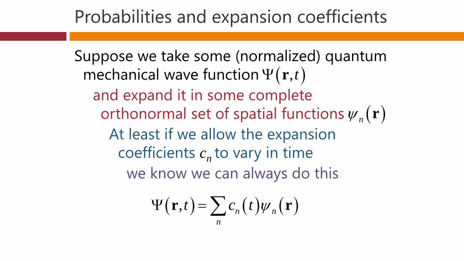
Suppose we take some (normalized) quantum mechanical wave function
and expand it in some complete orthonormal set of spatial functions
At least if we allow the expansion coefficients cn to vary in time
we know we can always do this
,t r
n r
, n nn
t c t r r

Probabilities and expansion coefficients
Then the fact that is normalized means we know the answer for the normalization integral
Because of the orthogonality of the basis functions only terms with survive the integration
Because of the orthonormality of the basis functions the result from any such term will simply be
Hence we have
,t r
2 3 3, 1n n m mn m
t d c t c t d
r r r r r
n m
2nc t
2 1nn
c

Measurement postulate
On measurement of a statethe system collapses into the nth
eigenstate of the quantity being measuredwith probability
In the expansion of the state in the eigenfunctions
of the quantity being measuredcn is the expansion coefficient
of the nth eigenfunction
2n nP c

Expectation value of the energy
Suppose do an experiment to measure the energy E of some quantum mechanical system
We could repeat the experiment many timesand get a statistical distribution of results
Given the probabilities Pn of getting a specific energy eigenstate, with energy En
we would get an average answer
where we call this average the “expectation value”
2n n n n
n n
E E P E c E
Energy expectation value example
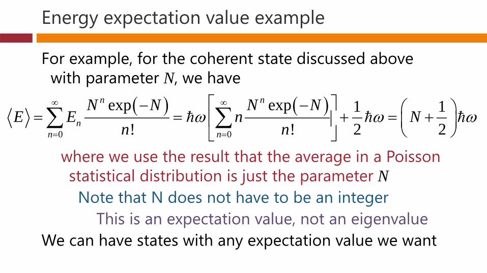
For example, for the coherent state discussed above with parameter N, we have
where we use the result that the average in a Poisson statistical distribution is just the parameter N
Note that N does not have to be an integerThis is an expectation value, not an eigenvalue
We can have states with any expectation value we want
0 0
exp exp 1 1! ! 2 2
n n
nn n
N N N NE E n N
n n

Stern-Gerlach experiment
This apparatus has a non-uniform magnetic fieldlocally stronger near the
North pole magnet facebecause it is narrower
N
S
magnet North pole
magnet South pole
screen
magnetic field more
concentrated here
than here

Stern-Gerlach experiment
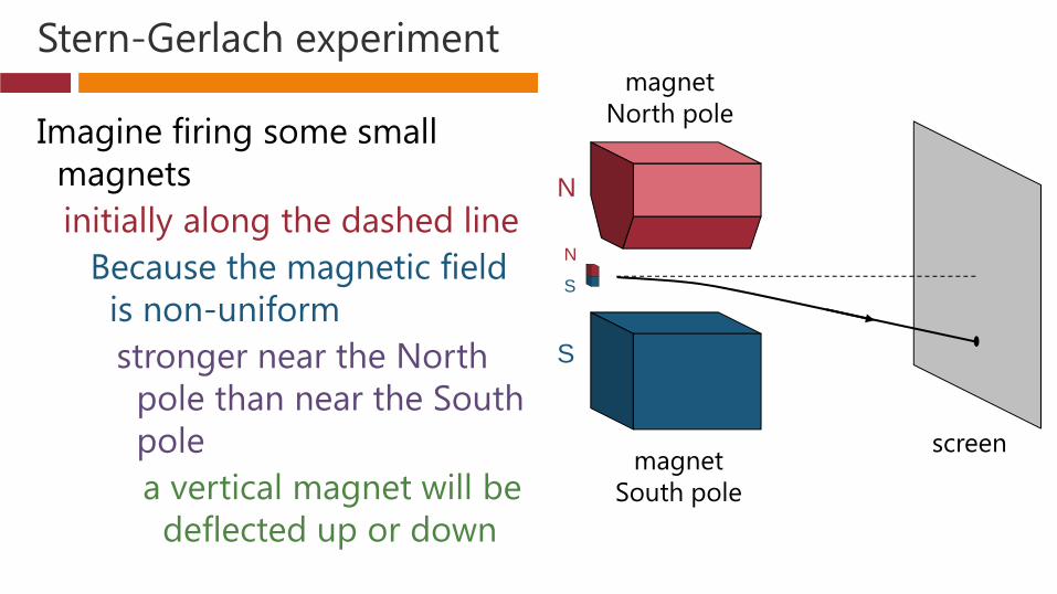
Imagine firing some small magnets initially along the dashed line
Because the magnetic field is non-uniformstronger near the North
pole than near the South polea vertical magnet will be
deflected up
N
S
N
S
magnet North pole
magnet South pole
screen
Stern-Gerlach experiment
Imagine firing some small magnets initially along the dashed line
Because the magnetic field is non-uniformstronger near the North
pole than near the South polea vertical magnet will be
deflected up or down
S
N
N
S
magnet North pole
magnet South pole
screen

Stern-Gerlach experiment
A horizontally-oriented magnet will not be deflected
SN
N
S
magnet North pole
magnet South pole
screen

Stern-Gerlach experiment
A horizontally-oriented magnet will not be deflectedand magnets of other
orientationsshould be deflected by intermediate amounts
After “firing” many randomly oriented magnetswe should end up with a line
on the screen
N
S
magnet North pole
magnet South pole
screen
?
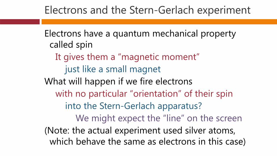
Electrons and the Stern-Gerlach experiment
Electrons have a quantum mechanical property called spin
It gives them a “magnetic moment”just like a small magnet
What will happen if we fire electronswith no particular “orientation” of their spin
into the Stern-Gerlach apparatus?We might expect the “line” on the screen
(Note: the actual experiment used silver atoms, which behave the same as electrons in this case)

Stern-Gerlach experiment
With electronswe get two dots!
“Explanation”We are measuring the vertical
component of the spinThere are two eigenstatesof this componentup and down
so we have collapse to the eigenstates
N
S
magnet North pole
magnet South pole
screen
electrons


4.3 Measurement and expectation values
Slides: Video 4.3.3 Expectation values and operators
Text reference: Quantum Mechanics for Scientists and Engineers
Sections 3.9 – 3.10

Measurement and expectation values
Expectation values and operators
Quantum mechanics for scientists and engineers David Miller

Hamiltonian operator
In classical mechanics, the Hamiltonian is a function of position and momentum
representing the total energy of the systemIn quantum mechanical systems that can be analyzed by
Schrödinger’s equationwe can define the entity
so we can write the Schrödinger equations as
and
2ˆ ,2
H V tm
2
r
,ˆ ,t
H t it
r
r H E r r
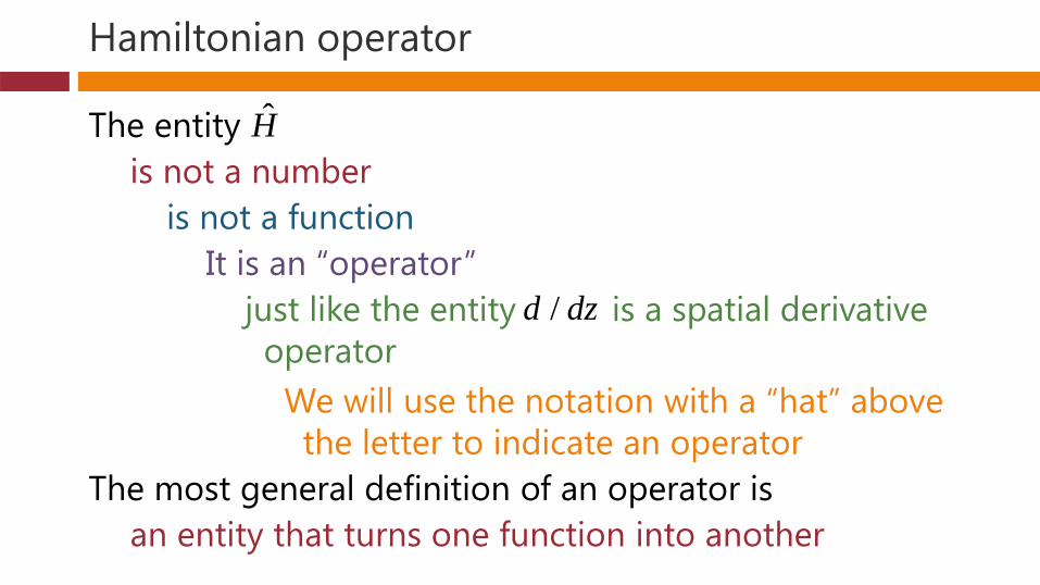
Hamiltonian operator
The entityis not a number
is not a functionIt is an “operator”
just like the entity is a spatial derivative operator
We will use the notation with a “hat” above the letter to indicate an operator
The most general definition of an operator isan entity that turns one function into another
H
/d dz

Hamiltonian operator
The particular operator is called the Hamiltonian operator
Just like the classical Hamiltonian functionit is related to the total energy of the system
This Hamiltonian idea extends beyond the specific Schrödinger-equation definition we have so far
which is for single, non-magnetic particlesIn general, in non-relativistic quantum mechanics
the Hamiltonian is the operator related to the total energy of the system
H
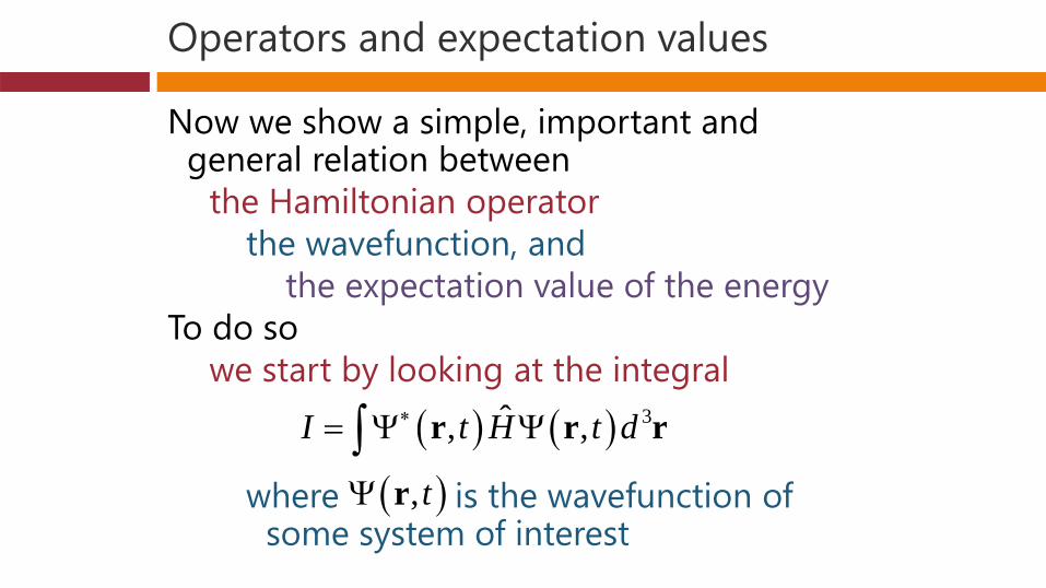
Operators and expectation values
Now we show a simple, important and general relation between
the Hamiltonian operatorthe wavefunction, and
the expectation value of the energyTo do so
we start by looking at the integral
where is the wavefunction of some system of interest
3ˆ, ,I t H t d r r r
,t r

Operators and expectation values
In looking at this integral
we will expand the wavefunction in the (normalized) energy eigenstates
So
3ˆ, ,I t H t d r r r
,t r
, n nn
t c t r r
2
2ˆ , , ,2
H t V t tm
r r r
n r
2
2 ,2 n n
nV t c t
m
r r n n nn
c t E r

Operators and expectation values
So the integral becomes
Because of the orthonormality of the basis functionsthe only terms in the double sum that survive
are the ones for which
so
But this is just the expectation value of the energy, so
3 3ˆ, , m m n n nm n
t H t d c t c t E d
r r r r r r
n r
n m
23ˆ, , n nn
t H t d E c r r r
3ˆ, ,E t H t d r r r
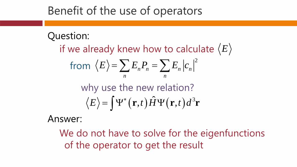
Benefit of the use of operators
Question:if we already knew how to calculate
from
why use the new relation?
Answer:We do not have to solve for the eigenfunctions of the operator to get the result
E2
n n n nn n
E E P E c
3ˆ, ,E t H t d r r r

4.3 Measurement and expectation values
Slides: Video 4.3.5 Time evolution and the Hamiltonian
Text reference: Quantum Mechanics for Scientists and Engineers
Section 3.11

Measurement and expectation values
Time evolution and the Hamiltonian
Quantum mechanics for scientists and engineers David Miller
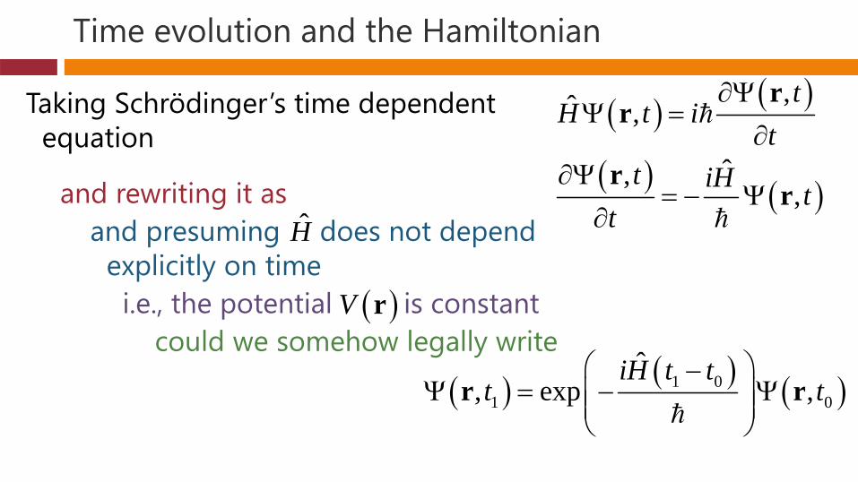
Time evolution and the Hamiltonian
Taking Schrödinger’s time dependent equation
and rewriting it asand presuming does not depend
explicitly on time i.e., the potential is constant
could we somehow legally write
,ˆ ,t
H t it
r
r
ˆ,
,t iH t
t
r
rH
V r
1 01 0
ˆ, exp ,
iH t tt t
r r

Time evolution and the Hamiltonian
Certainly, if the Hamiltonian operator here was replaced by a constant number
we could perform such an integration of
to get
1 01 0
ˆ, exp ,
iH t tt t
r r
ˆ,
,t iH t
t
r
r
H

Time evolution and the Hamiltonian
If, with some careful definition, it was legal to do thisthen we would have an operator that
gives us the state at time t1 directly from that at time t0To think about this “legality”
first we note that, because is a linear operatorfor any number a
Since this works for any functionwe can write as a shorthand
H
ˆ ˆ, ,H a t aH t r r
,t r
ˆ ˆHa aH
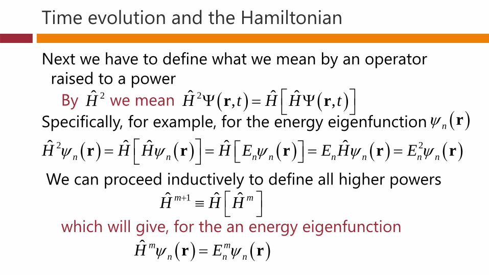
Time evolution and the Hamiltonian
Next we have to define what we mean by an operator raised to a power
By we meanSpecifically, for example, for the energy eigenfunction
We can proceed inductively to define all higher powers
which will give, for the an energy eigenfunction
2H 2ˆ ˆ ˆ, ,H t H H t r r n r
2 2ˆ ˆ ˆ ˆ ˆn n n n n n n nH H H H E E H E r r r r r
1ˆ ˆ ˆm mH H H
ˆ m mn n nH E r r
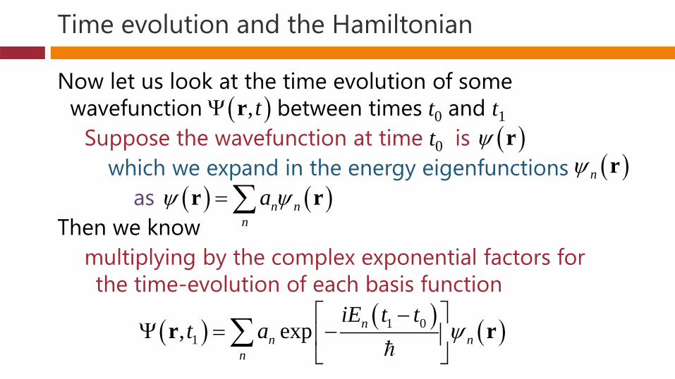
Time evolution and the Hamiltonian
Now let us look at the time evolution of some wavefunction between times t0 and t1
Suppose the wavefunction at time t0 iswhich we expand in the energy eigenfunctions
as Then we know
multiplying by the complex exponential factors for the time-evolution of each basis function
,t r r
n r n n
n
a r r
1 01, exp n
n nn
iE t tt a
r r
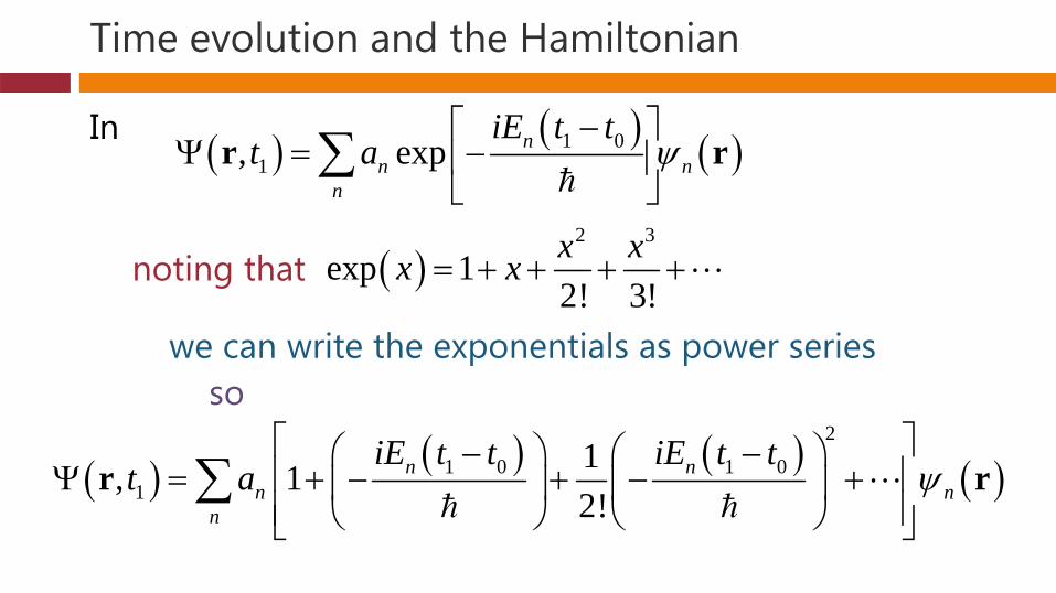
Time evolution and the Hamiltonian
In
noting that
we can write the exponentials as power seriesso
1 01, exp n
n nn
iE t tt a
r r
2 3
exp 12! 3!x xx x
2
1 0 1 01
1, 12!
n nn n
n
iE t t iE t tt a
r r

Time evolution and the Hamiltonian
In
because we showed thatwe can substitute to obtain
2
1 0 1 01
1, 12!
n nn n
n
iE t t iE t tt a
r r
ˆ m mn n nH E r r
2
1 0 1 01
ˆ ˆ1, 12!n n
n
iH t t iH t tt a
r r

Time evolution and the Hamiltonian
With
because the operator and all its powers commute with scalar quantities (numbers) we can rewrite
H
2
1 0 1 01
ˆ ˆ1, 12!n n
n
iH t t iH t tt a
r r
2
1 0 1 01
2
1 0 1 00
ˆ ˆ1, 12!
ˆ ˆ11 ,2!
n nn
iH t t iH t tt a
iH t t iH t tt
r r
r

Time evolution and the Hamiltonian
So, provided we define the exponential of the operator in terms of a power series, i.e.,
then we can write our preceding expression as
2
1 0 1 0 1 0ˆ ˆ ˆ1exp 1
2!iH t t iH t t iH t t
1 01 0
ˆ, exp ,
iH t tt t
r r

Time evolution and the Hamiltonian
Hence we have established that there is a well-defined operator that
given the quantum mechanical wavefunction or “state” at time t0
will tell us what the state is at a time t1
1 01 0
ˆ, exp ,
iH t tt t
r r
