2d heat conduction fem

7/29/2019 2d Heat Conduction Fem

http://slidepdf.com/reader/full/2d-heat-conduction-fem 1/8

3.5 Heat Conduction

Heat conduction is defined as the transfer of thermal energy from the more

energetic particles of a medium to the adjacent less energetic ones. Conduction can take

place in liquids and gases as well as solids provided. Heat transfer problems are often

classified as being steady or transient. It is also being classified as one-dimensional, two-

dimensional, or three-dimensional depending on the level accuracy desired.

In this analysis, two-dimensional heat conduction problem is considered. So, in

terms of a single independent variable, T, the governing equation of the heat conduction

is,

0=∂∂

−+

∂∂

∂∂

+

∂∂

∂∂

t

T cQ

y

T k

y x

T k

x ρ

where the heat fluxes are,

x

T

k q x ∂

∂

−= y

T

k q y ∂

∂

−=

and, c = specific heat

ρ = density

Applying the boundary condition of,

oT T = on C1 (fixed temperature ; Dirichlet boundary condition)

and,

qnT k =∂∂− on C2 (fixed heat flux ; Neumann boundary condition)

for convective heat transfer boundary condition,

)( f s T T hn

T k −=∂∂

− on C2



3.6 Galerkin Weighted Residual Method

In this analysis, the Galerkin method for the development of finite elements

algorithms is applied. The residual provides the error in the satisfaction of the equation.

Consider the residual equation,

Q y

T k

y x

T k

x R s +

∂∂

∂∂

+

∂∂

∂∂

=

where T contains trial functions and satisfies the boundary condition of oT T = at C1

and R s is a function of position in S.

To reduce the residual as close to zero as possible,

∫ = s

si ds RW 0 mi ,...,2,1=

where W i is set of arbitrary functions known as weighting functions,

A function ),( y xT that satisfies equation above for every function Wi in S is a weak

solution of differential equation.

For Neumann boundary condition,

qn

T k RC +∂

∂=2

∫ =+

∂∂

∂∂

+

∂∂

∂∂

si dsQ

y

T k

y x

T k

xW 0)(



where R C2 is the residual on C2.

Thus,

∫ =2

2 0C

C idc RW mi ,...,2,1=

where iW is the weighting functions on C2.

∫ =+∂∂

20)(

C i dcq

n

T k W

Combining R s and R C2 , the weak form,

∫ ∫ =+∂∂

++

∂∂

∂∂

+

∂∂

∂∂

20)()(

C i

si dcq

n

T k W dsQ

y

T k

y x

T k

xW

where this form will be simplified using Green’s Lemma theorem.

3.7 Green’s Lemma Theorem

Green's theorem gives the relationship between a line integral around a simple

closed curve C and a double integral over the plane region R bounded by C . It is the two-

dimensional special case of the more general Stokes' theorem, and is named after British

scientist George Green.

This theorem is mostly used to solve two-dimensional flow integrals, stating that

the sum of fluid outflows at any point inside a volume is equal to the total outflow

summed about an enclosing area. In this application, Green’s theorem will simplify the

integration of partial differential equation concerned.

http://www.answers.com/topic/line-integral-2

http://www.answers.com/topic/multiple-integral

http://www.answers.com/topic/stokes-theorem


http://www.answers.com/topic/united-kingdom

http://www.answers.com/topic/george-green

http://www.answers.com/topic/multiple-integral


http://www.answers.com/topic/united-kingdom

http://www.answers.com/topic/george-green

http://www.answers.com/topic/line-integral-2



From the previous form,

∫ ∫ =+∂∂

++

∂∂

∂∂

+

∂∂

∂∂

20)()(

C i

si dcq

n

T k W dsQ

y

T k

y x

T k

xW

Apply the Green’s Lemma and the equation become,

∫ ∫ ∫ ∫ +=+

∂∂

+∂∂

++

∂∂

∂∂

+∂∂

∂∂

21 20)()(

C C C ii

si

s

ii dcqn

T k W dc

n

T k W QdxdyW dxdy

y

T k

y

W

x

T k

x

W

Now, limit the choice of weighting functions as,

0=iW on C1

ii W W −= on C2

Thus,

∫ ∫ ∫ =+−

∂∂

∂∂

+∂∂

∂∂

s C ii

s

ii dcqW QdxdyW dxdy y

T k

y

W

x

T k

x

W

20

In order to obtain the approximation of the solution from the above weak form equation,

it is need to choose appropriate trial functions, ),( y x N i to represent the real solution.

∑∞

=

+=1

),(),(i

iio y x N C C y xT

Employing the Galerkin Method,

),(),( y x N y xW ii =

Thus,



∫ ∫ ∫ =+−

∂∂

∂∂

+∂∂

∂∂

s C ii

s

ii dcq N Qdxdy N dxdy y

T k

y

N

x

T k

x

N

20

3.8 2D Triangular Elements

The triangular elements describing a two-dimensional temperature distribution are

better suited to approximate curved boundaries. A triangular element is defined by three

nodes.

Therefore, the variation of a dependent variable, such as temperature, over the

triangular region is given by,

Y a X aaT e

321

)( ++=

Figure 3.2

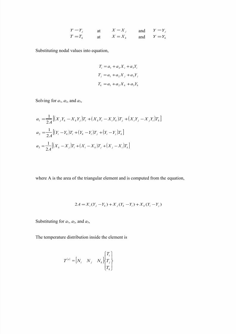
Considering the nodal temperatures as shown in figure, the following conditions must be

satisfied:

iT T = at i X X = and iY Y =

X Y

T j

T k

X Y

X i Y i

T i



jT T = at j X X = and jY Y =

k T T = at k X X = and k Y Y =

Substituting nodal values into equation,

iii Y a X aaT 321 ++=

j j j Y a X aaT 321 ++=

k k k Y a X aaT 321 ++=

Solving for a1, a2, and a3,

( ) ( ) ( )[ ]k i j ji jk iik i jk k jT Y X Y X T Y X Y X T Y X Y X

Aa −+−+−=

21

1

( ) ( ) ( )[ ]k ji jik ik i T Y Y T Y Y T Y Y A

a −+−+−=2

12

( ) ( ) ( )[ ]k i j jk ii jk T X X T X X T X X A

a −+−+−=2

13

where A is the area of the triangular element and is computed from the equation,

)()()(2 jik ik jk ji Y Y X Y Y X Y Y X A −+−+−=

Substituting for a1, a2, and a3,

The temperature distribution inside the element is

( ) [ ]

=

k

j

i

k ji

e

T

T

T

N N N T



where the shape function k ji N N N ,, are,

( )Y X A

N iiii δ β α ++=21

( )Y X A

N j j j j δ β α ++=2

1

( )Y X A

N k k k k δ β α ++=2

1

jk k ji Y X Y X −=α k ji Y Y −=β jk i X X −=δ

k iik j Y X Y X −=α ik j Y Y −=β k i j X X −=δ

i j jik Y X Y X −=α jik Y Y −=β i jk X X −=δ

Thus,

∫

∂∂

∂∂

+∂∂

∂∂

= s

ji jiij dxdy

y

N k

y

N

x

N k

x

N K

[ ]∫ += s

ji ji dxdy Ak δ δ β β

24

[ ] ji ji A

k δ δ β β +=

43,2,1, = ji

Complete element matrix,

++++++

+++

=k k k k jk jk ik ik

k jk j j j j ji ji j

k ik i ji jiiiii

A K

δ δ β β δ δ β β δ δ β β δ δ β β δ δ β β δ δ β β

δ δ β β δ δ β β δ δ β β 1

and K is symmetric.

Element load vector, F,

qQ f f f +=



where,

=

= ∫ 1

1

1

3

QAds

N

N

N

Q f s

k

j

i

Q and dc N q f C

q ∫ −=2

If side ij of the triangle is subjected to the Neumann boundary condition with a uniform

flux, q , then,

dc N

N

q f f ijC

j

i

qq ij ∫

−==

2

0

dc L

qij

−=

0

11

2

where Lij is the length of element side ij.

2d heat conduction fem

Documents