CAVEAT-TR: A 2D hydrodynamic code with heat conduction

and radiation transport.

I. Implementation of the SSI method for heat conduction

Mikhail M. BaskoGSI, Darmstadt; on leave from ITEP, Moscow∗

Joachim A. Maruhn and Anna TauschwitzFrankfurt University, Frankfurt

∗Electronic address: basko@itep.ru

CAVEAT-TR 2007 2

CAVEAT-TR 2007 3

Contents

1. Introduction 5

2. Energy equation with thermal conduction and radiation transport 6

3. Lagrangian phase of the algorithm 83.1. The general 3D case 83.2. Reduction to the 2D case 9

4. General scheme of the SSI algorithm 11

5. SSI realization for heat conduction 135.1. General scheme 135.2. Formulae for explicit deposition rates WT and total fluxes Hijm 145.3. Flux limiting 155.4. Formulae for coefficients DT 165.5. Formulae for the energy corrections δT 165.6. Weight coefficients for the energy correction 175.7. Time step control 185.8. Boundary conditions 19

1. Physical boundaries 192. Block interfaces 20

6. Test problems 236.1. Problem 1: one-dimensional non-linear heat wave 236.2. Problem 2: a spherical heat wave from an instantaneous point source 286.3. Problem 3: a planar shock wave with heat conduction 31

A. CAVEAT interpolation schemes 331. Vertex temperatures 33

a. 1D interpolation 33b. 2D interpolation 34

2. Face-centered heat flux 353. Face-centered conduction coefficient 37

References 37

CAVEAT-TR 2007 4

CAVEAT-TR 2007 5

1. INTRODUCTION

The PHELIX laser at GSI (Darmstadt) is currently able to deliver about 500 joules ofenergy in 2–3 ns long pulses for plasma physics experiments. In future, the pulse energyis planned to be increased up to 3.6 kJ. A combination of intense laser and ion beams atGSI offers a unique possibility to study fundamental properties of matter at high energydensities. The PHELIX laser beam will be used to create hot plasmas with temperatures ofup to 1 keV by direct target irradiation. Indirect-drive schemes, based on various forms ofradiative hohlraums, hold out promise of well-controlled volumes of relatively dense quasi-uniform plasmas with temperatures T ∼ 100 eV. These laser-generated plasmas will be usedin a broad variety of experiments, some of them — like heavy ion stopping measurements inplasmas with T >∼ 10–50 eV — quite unique. Also, as a powerful X-ray backlighter emitter,laser-created plasmas should find their place in diagnostics of various experiments, wherematter is heated by intense ion beams. Investigation of hohlraum-created plasmas is of itsown interest in the context of inertial confinement fusion research.

Preparation and interpretation of all sorts of experiments, involving high-temperaturelaser plasmas, usually requires sophisticated two-dimensional (2D) — if not three-dimensional — hydrodynamic simulations with a proper account of heat conductionand spectral radiation transport. However, development of such a 2D RH (radiative-hydrodynamics) code still provides a major challenge from the point of view of computationalphysics. And especially so, if one expects such a code to be reasonably universal, fast andaccurate. Among a few 2D RH codes, existing presently in the world (like the well-knownLASNEX code at Livermore), only the MULTI-2D code, developed by R. Ramis (Madrid,Spain), is freely available and could, in principle, be employed for laser-plasma simulationsat GSI.

In numerical hydrodynamics there are two major competing approaches: one based onsome type of artificial (pseudo-) viscosity (av-schemes), and the other, Godunov-like ap-proach, based on some version of a Riemann solver [1]. From the physics point of view, aGodunov-like approach would always be preferable because it does not involve unphysicalviscosity and is automatically well-suited for accurate description of large density and pres-sure jumps. Once higher-order low-diffusion Godunov-like schemes had been developed [2],they were demonstrated to be superior to traditional av-schemes [1] in terms of accuracy aswell — at least to those of them which do not use specially developed techniques [3].

The MULTI-2D code by R. Ramis is based on a rather simple version of an av-schemefor an unstructured triangular mesh [4]. As a consequence, its capabilities in modellingcomplex two-dimensional flows (even in its later versions with a mesh adaptivity option)— like, for example, high-convergence implosions — appear rather limited. Also, radiationtransport in the distributed version of MULTI-2D is available only in a single-frequency-group approximation. An additional obstacle for any attempt to modify or upgrade theMULTI-2D code is the need to master the author’s original high-level programming language,in which the source code is written.

At the same time, very positive experience has been accumulated at GSI [5, 6] withthe 2D purely hydrodynamical code CAVEAT, originally developed at the Los Alamos Na-tional Laboratory [7] and written in the standard FORTRAN-77. CAVEAT is based on asecond-order Godunov-like scheme for a structured quadrilateral grid, and fully exploits theadvantages of the arbitrary Lagrangian-Eulerian (ALE) technique. Its numerical schemeproduces just the right amount of numerical diffusion, so that, for example, in the Rayleigh-

CAVEAT-TR 2007 6

Taylor unstable situations the shortest (on the scale of a single grid cell) wavelengths areconveniently suppressed, whereas at wavelengths of 8–10 grid cells the instability is quiteaccurately reproduced [5].

An important advantage of CAVEAT is that the scheme is able to maintain very accu-rately the inherent symmetry of the problem (due to the structured character of the meshand moderate amount of numerical diffusion) and, for example, follow symmetric implosionsdown to the radial convergence factors of ' 100 [6]. The code is well suited for treating multi-material problems with a broad selection of different equations of state; a special attentionis paid to accurate tracing of material interfaces. Another major advantage of CAVEAT isa possibility to handle topologically complex situations, where the computational domainis comprised of many mutually bordering topologically quadrilateral blocks, each having alocally structured mesh. Building up on this positive experience, a decision was made by thepresent authors to undertake a challenging project of upgrading the original 2D CAVEATcode to a version which includes both the thermal conduction and the spectral radiation

transport. The new version has been named CAVEAT-TR.The original CAVEAT scheme is based on cell-centered values for all principal dynamic

variables, one of which is the total (internal + kinetic) fluid energy density E. For ther-mal conduction and radiation transport, a more natural principal variable would be mattertemperature T , for which vertex-centered values are needed. The difficulties associatedwith combining these two approaches are extensively discussed in Ref. [8]. In this part I ofthe report on CAVEAT-TR we describe implementation of the symmetrical semi-implicit(SSI) method [9] for treating thermal conduction. After introduction of two complementarycriteria for time-step control, the SSI method was found to work quite accurately and effi-ciently within the general CAVEAT scheme. The adopted reinterpolation scheme from thecell-centered to vertex-centered temperature values is demonstrated to provide more thansufficient accuracy in describing the propagation of non-linear heat fronts.

2. ENERGY EQUATION WITH THERMAL CONDUCTION AND RADIATION

TRANSPORT

Heat conduction and radiation transport (the latter — in the simplest approximation ofinstantaneous energy redistribution) appear only in the energy equation

∂(ρE)

∂t+ div [(ρE + p)~u] = − div

(

~h + ~hr

)

+ Q (2.1)

CAVEAT-TR 2007 7

of the full system of the hydrodynamic equations. Here

ρ = ρ(t, ~x) is the fluid density [g cm−3],

E = e +u2

2is the mass-specific total energy [erg g−1],

e = e(t, ~x) is the mass-specific internal energy [erg g−1],

~u = ~u(t, ~x) is the fluid velocity [cm s−1],

p = p(ρ, e) is the fluid pressure [erg cm−3],

Q = Q(t, ~x) = ρq is the volume-specific external heating rate [erg cm−3 s−1],

q = q(t, ~x) is the mass-specific external heating rate [erg g−1 s−1],

T = T (ρ, e) is the fluid temperature [eV],~h = −κ∇T is the area-specific heat flux [erg cm−2 s−1],

κ = κ(ρ, T ) is the heat conduction coefficient [erg cm−1 s−1 eV−1],

~hr =

∞∫

0

dν

∫

4π

~ΩI d~Ω is the area-specific radiation energy flux [erg cm−2 s−1],

I = I(~x, ν, ~Ω) is the radiation intensity [erg cm−2 s−1 ster−1 eV−1],

ν is the photon frequency [eV],~Ω is the unit vector in the direction of photon propagation,

d~Ω is the solid angle element.

(2.2)

At each time t the radiation intensity I(~x, ν, ~Ω) is calculated by solving the time-independent transport equation

~Ω · ∇I = kν (Ipl − I) , (2.3)

where

kν = kν(ν, ρ, T ) is the radiation absorption coefficient [cm−1],

Ipl = 5.0404 × 1010 ν3

exp(ν/T ) − 1is the Planckian intensity [erg cm−2 s−1 ster−1 eV−1].

(2.4)Note that kν is the full — i.e. corrected for stimulated emission — absorption coefficient. Thesimplest version (2.3) of the transport equation is written under the assumptions that (i) ateach time a negligible amount of energy resides in the radiation field, and (ii) no momentumis transferred by radiation, i.e. radiation pressure can be ignored. This approximation maybe called the approximation of instantaneous energy redistribution (IRD), and is in thissense analogous to heat conduction: in the optically thick case it is equivalent to addingthe radiative heat conduction coefficient κr = 4

3aclRT 3 to the molecular (electron) heat

conduction coefficient κ; here a is a constant in the expression aT 4 [erg cm−3] for theequilibrium radiative energy density, c is the speed of light, and lR = lR(ρ, T ) is the Rosselandmean free path of photons.

CAVEAT-TR 2007 8

3. LAGRANGIAN PHASE OF THE ALGORITHM

3.1. The general 3D case

In the CAVEAT code all the energy deposition and redistribution is accomplished duringthe Lagrangian phase (L-step) of the computational cycle; a computational cycle is a singletime step, during which all the principal variables are advanced in time from t to t + ∆t.Below the quantities in a cell (i, j) at the end of the Lagrangian phase are marked with abar, like eij, Eij, Tij . . .

In the Lagrangian phase the mass-specific total energy E is advanced according to theintegral form of the energy equation (2.1)

d

dt

∫

Vij

ρE dV = −∫

Sij

p ~u · ~n dS −∫

Sij

(~h + ~hr) · ~n dS +

∫

Vij

ρq dV, (3.1)

where Vij is the Lagrangian volume of the mesh cell (i, j), Sij is its surface area, and ~n isthe outward unit normal to the cell surface. Note that the cell mass

Mij =

∫

Vij

ρ dV (3.2)

is conserved in the L-step, i.e. dMij/dt = 0. By definition, the following relationships arealways fulfilled

Eij =1

Mij

∫

Vij

ρE dV, qij =1

Mij

∫

Vij

ρq dV. (3.3)

The density ρij in cell (i, j) is calculated from the relationship

ρij =Mij

Vij. (3.4)

The mass-specific total energy Eij of cell (i, j) is advanced in the L-step according to thefollowing finite-difference approximation to Eq. (3.1)

Eij = Eij + ∆t

(

Wp,ij + WT,ij + Wr,ij

Mij+ qij

)

, (3.5)

where the corresponding energy deposition powers (in [erg s−1]) in cell (i, j) are given by

Wp,ij = −∫

Sij

p ~u · ~n dS, WT,ij = −∫

Sij

~h · ~n dS, Wr,ij = −∫

Sij

~hr · ~n dS. (3.6)

The cell volume Vij is advanced in the L-step according to the equation

dVij

dt=

∫

Vij

div ~u dV =

∫

Sij

~u · ~n dS. (3.7)

CAVEAT-TR 2007 9

Correspondence with the code variables:

ρij = RHO(I,J) intensive, mass density;

pij = PR(I,J) intensive, pressure;

Vij = VOL(I,J) extensive, cell volume;

Mij = CM(I,J) extensive, cell mass; conserved in the L-step;

eij = SIE(I,J) intensive, mass-specific internal energy;

eij = SIEL(I,J) intensive;

Eij = TE(I,J) intensive;

Eij = TEL(I,J) intensive;

qij = QDEPO(I,J) intensive, mass-specific heating rate;

3.2. Reduction to the 2D case

Two-dimensional flows are described by using two different versions of coordinate systems:(i) Cartesian, when the internal CAVEAT coordinates are (x1, x2) = (x, y), and (ii) cylin-drical, when the internal coordinates are either (x1, x2) = (r, z), or (x1, x2) = (z, r); here ris the cylindrical radius. These two different mesh geometries are combined by introducinga generalized radius

R =

1, (x1, x2) = (x, y), Cartesian, IRADIAL=0,

x1, (x1, x2) = (r, z), cylindrical 1, IRADIAL=1,

x2, (x1, x2) = (z, r), cylindrical 2, IRADIAL=2.

(3.8)

Then, the 3D volume Vij in 2D problems becomes either a volume per unit length along thez-axis in the Cartesian case, or a volume per steradian of the azimuth angle in the axiallysymmetric case. To get the full 3D volume in the axially symmetric case, one has to multiplythe 2D volume Vij by 2π. The same pertains to the surface areas Sij, and to all extensivephysical quantities.

Accordingly, all the volume and surface integrals are transformed as follows. The integralof any scalar intensive quantity q over the cell volume is cast in a form

∫

Vij

q dV =

∫

Aij

q R dx1 dx2, (3.9)

where Aij is the surface area of the mesh cell (i, j) on the x1, x2-plane; remind that theinternal coordinates x1, x2 are treated as orthogonal Cartesian.

A corresponding surface integral is then given by∫

Sij

q dS =

∫

Lij

q R dλ, (3.10)

where Lij is the perimeter of the mesh cell (i, j) on the x1, x2-plane, and dλ is the lengthelement along this perimeter. For quadrangular cells with straight sides the integral (3.10)

CAVEAT-TR 2007 10

is approximated as a sum over its four sides (faces)

∫

Lij

q R dλ =4∑

α=1

qf,α Λα, (3.11)

where qf,α is the face-centered value of q, and

Λα =

∫

face α

R dλ. (3.12)

cell (i,j)

face (i,j,1)

face

(i,

j,2)

(i,j+1)

(i+1,j)(i,j)

nf,ij1

nf,ij2

FIG. 3.1: Numbering of vertices, cells and faces in CAVEAT.

For straight-line faces the integral in (3.12) is calculated exactly. In the CAVEAT nomen-clature the faces are numbered after the vertices from which they originate; for each vertex(i, j) there are two faces ascribed to it; face (i, j, 1) connects the vertex (i, j) to (i + 1, j);face (i, j, 2) connects the vertex (i, j) to (i, j +1) (see Fig. 3.1). On each face (i, j, m) a unitnormal vector ~nf,ijm is defined, which points in the positive direction of the alternative co-ordinate x3−m; here m = 1, 2. This normal vector should not be mixed (!) with the outwardnormal ~n to the cell surface, used in the formulae of the previous section. The quantity Λijm

is called the area of the face (i, j, m); its values are given by

Λij1 = 12(Rij + Ri+1,j) |~xi+1,j − ~xij| ,

Λij2 = 12(Rij + Ri,j+1) |~xi,j+1 − ~xij| ;

(3.13)

here ~x = x1; x2 is the vector with coordinates x1, x2, and ~xij represents coordinates of themesh vertex (ij) (see Fig. 3.1).

CAVEAT-TR 2007 11

Correspondence with the code variables:

x1,ij = XV(I,J,1) x1-coordinate of vertex (i, j);

x2,ij = XV(I,J,2) x2-coordinate of vertex (i, j);

nf,ijm,1 = FN(I,J,M,1) x1-component of the unite normal vector ~nf,ijm; calcu-lated in subroutine GEOM;

nf,ijm,2 = FN(I,J,M,2) x2-component of the unite normal vector ~nf,ijm; calcu-lated in subroutine GEOM;

Λijm = FA(I,J,M) (> 0) area of face (i, j, m); calculated in subroutine GEOM;

4. GENERAL SCHEME OF THE SSI ALGORITHM

When applying the SSI method to Eq. (3.5), we split the terms on its right-hand side intotwo groups: (i) the p dV -work, represented by the ∆tWp,ij/Mij term, is treated explicitly(i.e. taken over unaltered from the original CAVEAT version) and remains untouched by theSSI scheme; (ii) the remaining ∆t WT,ij/Mij, ∆t Wr,ij/Mij, and ∆t qij terms are combinedinto a joint SSI step. As discussed below, splitting into separate SSI steps with respect toheat conduction and radiative transport might seriously undermine the code’s capability totreat laser-heating problems.

Then, the L-step for the energy equation is accomplished according to the followingfinite-difference representation

Eij = Eij +∆t

Mij

Wp,ij +∆t

Mij

(

WT,ij + Wr,ij

)

+ qij∆t +δT,ij + δr,ij

Mij

. (4.1)

The cell deposition powers WT,ij, Wr,ij [erg s−1] are defined in Eq. (3.6). Tilde above thesequantities means that they are evaluated by using not the “old” (i.e. assigned before the startof the new computational cycle) temperatures Tij but the SSI-advanced “new” temperatures

Tij (for more details see the next section); note that the SSI-advanced temperatures Tij arenot the same as the L-step-advanced temperatures Tij. The values WT,ij, Wr,ij without atilde are calculated by using the old temperatures Tij; it is these values that would havebeen used under the explicit treatment of heat conduction and radiation transport. Theterms δT,ij, δr,ij [erg] in Eq. (4.1) are the energy corrections from the previous time step,originating from the energy disbalance inherent in the SSI method [9]. These quantities donot participate in calculation of the SSI-advanced temperatures Tij and deposition powers

WT (r),ij .When adding the amount of energy δT (r),ij to cell (i, j), it should be kept in mind that

δT (r),ij was calculated in the previous hydro cycle. Since due to mesh rezoning the cell massMij may change from cycle to cycle, the “old” energy correction, imposed on a “new” massMij may, in principal, lead to a temperature overshoot and potential instability. Neverthe-less, we choose this method, based on passing to a new cycle the absolute energy correctionδT (r),ij rather than the mass-specific quantity δT (r),ij/Mij, because it is globally conservative,and because it is difficult to propose a reasonable alternative for a purely Eulerian mesh.

Probably, the energy corrections δT,ij and δr,ij should be also subjected to the remapping

procedure at the rezoning phase!

CAVEAT-TR 2007 12

Now, having split the physical processes into those participated and not participating inthe SSI step, we have the following equation for calculating the SSI-advanced temperaturesTij and specific internal energies eij:

eij − eij =∆t

Mij

(

WT,ij + Wr,ij + qijMij

)

+δT,ij + δr,ij

Mij. (4.2)

Because the SSI step does not include the hydro motion, we use the specific internal energieseij instead of Eij, and we can relate the change in e to the change in T by invoking the heatcapacity cV (per unit mass) at constant volume,

eij − eij = cV,ij τij, (4.3)

whereτij = Tij − Tij (4.4)

is the principal unknown quantity to be determined at the SSI step. The heat capacity cV

is calculated from the old (i.e. available at the start of the cycle) values of e, ρ, T .After an appropriate linearization (required, in particular, for the radiative transport),

general expressions for WT (r),ij can be cast in the form

WT,ij = −DT,ijτij + WT,ij, Wr,ij = −Dr,ijτij + Wr,ij, (4.5)

where the coefficients DT,ij are determined by mesh geometry and the conduction coefficientsκij, Dr,ij — by mesh geometry, opacities kν,ij, old temperatures Tij and densities ρij. Notethat by their physical meaning the coefficients DT (r),ij must be non-negative because, when acell (i, j) is overheated and τij is large, both heat conduction and radiative transport shouldlead to the cooling of this same cell (i, j).

Having substituted Eqs. (4.5) and (4.3) into Eq. (4.2), we obtain

τij =(WT,ij + Wr,ij + qijMij)∆t + δT,ij + δr,ij

cV,ijMij + ∆t(DT,ij + Dr,ij), (4.6)

and the final equation for the L-step in the specific total energy

Eij = Eij +∆t

MijWp,ij + cV,ijτij. (4.7)

Obviously, for DT,ij = Dr,ij = 0 we recover the “underlying” explicit scheme for heatconduction and radiation transport.

Equation (4.6) clearly illustrates the advantages of combining conduction, radiation andexternal heating into a single SSI step (i.e. not splitting with respect to each individualprocess). If, for example, laser heating occurs in a thin layer, then this layer rapidly becomesvery hot with large values of either DT,ij or Dr,ij (or both); then, once ∆t(DT,ij + Dr,ij) >cV,ijMij, Eq. (4.6) naturally prevents the heated cells from being “overheated” — whichwould occur with a separate and explicit treatment of the heating source qij.

CAVEAT-TR 2007 13

Correspondence with the code variables:

∆t = DTHYDRO time step;

Tij = TEMP(I,J) intensive, temperature;

κij = TCOND(I,J) intensive, conduction coefficient;

cV,ij = CV(I,J) intensive, mass-specific heat capacity;

eij − eij = DTESSI(I,J) intensive, mass-specific internal energy increment;

δT,ij + δr,ij = ECORSSI(I,J) extensive, energy correction to cell (i, j) for the next cycle;

5. SSI REALIZATION FOR HEAT CONDUCTION

5.1. General scheme

As explained in section 4, implementation of the SSI algorithm for heat conduction re-quires calculation of three cell-centered quantities: WT,ij, DT,ij and δT,ij. Bar over δT,ij

means that this quantity will only be used in the next cycle. The deposition power WT,ij

for cell (i, j) can be written as

WT,ij = Hij1 + Hij2 − Hi,j+1,1 − Hi+1,j,2, (5.1)

WT,ij = Hij1 + Hij2 − Hi,j+1,1 − Hi+1,j,2,

where

Hijm = +

∫

face (i,j,m)

(κ∇T · ~n) R dλ = −∫

face (i,j,m)

(κ∇T · ~nf,ijm) R dλ, m = 1, 2, (5.2)

is the total (in [erg s−1]) conductive energy flux across the face (i, j, m) (see Fig. 5.1). Ina finite difference version of Eq. (5.2) Hijm is a linear function of the temperatures Tij,Ti±1,j, Ti,j±1, Ti±1,j±1, associated with the centers of the cell (i, j) and the neighboring cells(i ± 1, j), (i, j ± 1), (i ± 1, j ± 1).

To be able to calculate the coefficients DT,ij, we have to single out in Eq. (5.2) the explicitdependence on two face-adjacent temperatures:

Hij1 = −aij1Tij + bij1Ti,j−1 +∑′

c1αTα, (5.3)

Hij2 = −aij2Tij + bij2Ti−1,j +∑′′

c2αTα. (5.4)

In the above expressions the summation∑

′ is performed over all the participating temper-atures other than Tij and Ti,j−1, the summation

∑

′′ — over all participating temperaturesother than Tij and Ti−1,j. By their physical meaning, the coefficients aijm and bijm must beboth non-negative. The algorithm for evaluation of the coefficients aijm and bijm depends on

a particular scheme chosen for finite-difference approximation of the heat flux ~h = −κ∇T .Representation (5.3) leads us to the following expressions for the semi-implicit fluxes Hα

CAVEAT-TR 2007 14

(i,j+1)

(i+1,j)(i,j)

Hij1

Hij2

Hi,j+1,1

Hi+1,j,2T

ijTi+1,j

Ti,j-1

Ti-1,j

Ti,j+1

(i+1,j+1)

FIG. 5.1: Nomenclature of heat fluxes across the faces of cell (i, j).

that should be used to calculate the semi-implicit deposition power WT,ij:

Hij1 = −aij1 τij + Hij1, (5.5)

Hij2 = −aij2 τij + Hij2, (5.6)

Hi,j+1,1 = bi,j+1,1 τij + Hi,j+1,1, (5.7)

Hi+1,j,2 = bi+1,j,2 τij + Hi+1,j,2. (5.8)

From Eqs. (5.5)–(5.8) and (5.1) we find

DT,ij = aij1 + aij2 + bi,j+1,1 + bi+1,j,2. (5.9)

Substituting Eqs. (5.1) and (5.9) into Eq. (4.6), we calculate τij.

Correspondence with the code variables:

aijm = WWAT(I,J,M) SSI coefficients;

bijm = WWBT(I,J,M) SSI coefficients;

Hijm = WWHT(I,J,M) extensive, total heat fluxes;

τij = DTESSI(I,J) intensive, temperature increments;

Tv,ij = TEMPV(I,J) intensive, vertex temperatures;

5.2. Formulae for explicit deposition rates WT and total fluxes Hijm

Equation (5.1) expresses WT,ij in terms of face-centered total fluxes Hijm, which, accord-ing to Eq. (A.20), are given by

Hijm =κf,ijmRf,ijm

|Jijm|[(

~λv,ijm · ~λc,ijm

)

∆Tv,ijm − |~λv,ijm|2∆Tijm

]

. (5.10)

CAVEAT-TR 2007 15

Here

∆Tijm =

Tij − Ti,j−1, m = 1,

Tij − Ti−1,j , m = 2,(5.11)

∆Tv,ijm =

Tv,i+1,j − Tv,ij , m = 1,

Tv,i,j+1 − Tv,ij , m = 2,(5.12)

vector ~λv,ij1 [or ~λv,ij2] connects vertex (i, j) with vertex (i + 1, j) [or (i, j + 1)], and vec-

tor ~λc,ij1 [or ~λc,ij2] connects cell center (i, j − 1) [or (i − 1, j)] with cell center (i, j);

see Fig. A.3. Jacobian Jijm is given by the vector product Jijm = ~λv,ijm ⊗ ~λc,ijm, i.e.|Jijm| = 2

∣

∣A+∆,ijm + A−

∆,ijm

∣

∣. Face-centered radii Rf,ijm are given by Eq. (A.16), and vertex-centered temperatures Tv,ij are given by Eqs. (A.10) and (5.19). When evaluating theface-centered conduction coefficients κf,ijm, a flux limiting condition

κf |∇T | ≤ hl (5.13)

is imposed as described in the following section; here hl > 0 [erg cm−2 s−1] is the maxi-mum allowed absolute value of the area-specific heat flux h. Physically, for electron heatconduction usually a formula is used

hl = finhneTe(Te/me)1/2, (5.14)

where the dimensionless inhibition factor finh ' 0.03–1.

5.3. Flux limiting

For each cell (i, j) a cell-centered flux limit hl,ij is defined. It is supposed to be calculatedtogether with the cell-centered conduction coefficient κf,ij in the thermodynamic part of thecode. Then the flux-limit-corrected face-centered conduction coefficient κijm is calculated as

κf,ijm = min

κf,ijm;hl,ijm

|g|ijm

, (5.15)

where κf,ijm is given by Eqs. (A.21) and (A.22),

hl,ij1 =

hl,i,j−1, Hij1 > 0,

hl,ij, Hij1 ≤ 0,(5.16)

hl,ij2 =

hl,i−1,j, Hij2 > 0,

hl,ij, Hij2 ≤ 0,(5.17)

and

|g|ijm =1

|Jijm|

[

∣

∣

∣

~λv,ijm

∣

∣

∣

2

∆T 2ijm +

∣

∣

∣

~λc,ijm

∣

∣

∣

2

∆T 2v,ijm − 2

(

~λv,ijm · ~λc,ijm

)

∆Tijm ∆Tv,ijm

]1/2

(5.18)is the absolute value of the face-centered temperature gradient ~g = (∇T )f [see Eq. (A.18)

below].

CAVEAT-TR 2007 16

5.4. Formulae for coefficients DT

Equation (5.9) expresses DT,ij in terms of face-centered coefficients aijm and bijm. Toobtain explicit formulae for aijm and bijm from Eq. (A.20), we cast the interpolation scheme(A.10) for the vertex temperatures Tv,ij in the form

Tv,ij = µ1,ij Tij + µ2,ij Ti−1,j + µ3,ij Ti−1,j−1 + µ4,ij Ti,j−1, (5.19)

which complies with the CAVEAT convention about numbering of the four cells that sur-round a vertex (i, j); see Fig. 5.2. Coefficients µα,ij are expressed in terms of the ξ, η values forthe vertex (i, j) and the cell-centered conduction coefficients κα in the surrounding four cells,as given by Eq. (A.10), with a restriction µα,ij > 0 and a provision of µ1,ij +µ2,ij +µ3,ij +µ4,ij.As a result, we calculate

aij1 =κf,ij1Rf,ij1

|Jij1|[

|~λv,ij1|2 +(

~λv,ij1 · ~λc,ij1

)

(+µ1,ij − µ2,i+1,j)]

, (5.20)

bij1 =κf,ij1Rf,ij1

|Jij1|[

|~λv,ij1|2 +(

~λv,ij1 · ~λc,ij1

)

(−µ4,ij + µ3,i+1,j)]

, (5.21)

for face 1, and

aij2 =κf,ij2Rf,ij2

|Jij2|[

|~λv,ij2|2 +(

~λv,ij2 · ~λc,ij2

)

(+µ1,ij − µ4,i,j+1)]

, (5.22)

bij2 =κf,ij2Rf,ij2

|Jij2|[

|~λv,ij2|2 +(

~λv,ij2 · ~λc,ij2

)

(−µ2,ij + µ3,i,j+1)]

, (5.23)

for face 2.

Tv,ij

µ1,ijTij

µ2,ijTi-1,j

µ3,ijTi-1,j-1

µ4,ijTi,j-1

12

3 4

FIG. 5.2: Numbering of cell-centered quantities used to evaluate vertex temperatures Tij .

5.5. Formulae for the energy corrections δT

Once the values of τij have been determined for the entire mesh, we can calculate theenergy correction δT,ij [erg], which is lost at the current L-step in cell (i, j), and which shouldbe added at the next time step. The energy disbalance arises from the fact that the flux

CAVEAT-TR 2007 17

Hij1, given by Eq. (5.5), is not equal to the flux Hij1, obtained from Eq. (5.7) by replacing jwith j − 1. As a result, we have a situation where energy either disappears or is created atcell interfaces. Since the flux discrepancy is proportional to ∆t, the energy correction willbe proportional to ∆t2.

If we denote the amount of energy disappearing at face (i, j, 1) as ed,ij1 ∆t [erg], then fromEqs. (5.5) and (5.7) it is easy to calculate that

ed,ij1 = aij1τij + bij1τi,j−1. (5.24)

Similarly, if the amount of energy lost at face (i, j, 2) is ed,ij2 ∆t, then

ed,ij2 = aij2τij + bij2τi−1,j. (5.25)

Finally, the energy compensation for the next time step is found to be

δT,ij = [χij1 ed,ij1 + χij2 ed,ij2 + (1 − χi,j+1,1) ed;i,j+1,1 + (1 − χi+1,j,2) ed;i+1,j,2] ∆t, (5.26)

where 0 ≤ χijm ≤ 1 is the fraction of the energy ed,ijm ∆t lost at face (i, j, m), which isascribed to the neighboring cell in the “forward” (i.e. along the normal ~nf,ijm) directionfrom this face (see Figs. 3.1 and 5.1). We assume that the weight χijm is proportionalto the total (not specific) heat capacity of the triangular region in cell (i, j), made up oftwo vertices of face (i, j, m) and of the cell center ~xc,ij (see Fig. 5.3); specific formulae aregiven in section 5 5.6 Similar weights are used in the original CAVEAT code to calculate theface-centered values κf,ijm of the conduction coefficient κ.

Rij R

i+1,j

Ri,j+1

Rc,ij

Rc,i,j-1

(a)

A−

Δ,ij1

A+

Δ,ij1

Rij R

i+1,j

Ri,j+1

Rc,ij

Rc,i-1,j

A−

Δ,ij2

(b)

A+

Δ,ij2

FIG. 5.3: Face-adjacent triangles used to calculate weights for splitting face-centered values between

the two adjacent cells.

5.6. Weight coefficients for the energy correction

For the weight coefficients χijm in Eq. (5.26) no formulae are available from the originalCAVEAT version. We evaluate them as

χijm =C+

∆,ijm

C+∆,ijm + C−

∆,ijm

(5.27)

CAVEAT-TR 2007 18

with a restriction of0 ≤ χijm ≤ 1; (5.28)

here

C+∆,ij1 =

1

3(Rij + Ri+1,j + Rc,ij) A+

∆,ij1 cV,ij ρij, (5.29)

C−

∆,ij1 =1

3(Rij + Ri+1,j + Rc,i,j−1) A−

∆,ij1 cV,i,j−1 ρi,j−1, (5.30)

C+∆,ij2 =

1

3(Rij + Ri,j+1 + Rc,ij) A+

∆,ij2 cV,ij ρij, (5.31)

C−

∆,ij2 =1

3(Rij + Ri,j+1 + Rc,i−1,j) A−

∆,ij2 cV,i−1,j ρi−1,j , (5.32)

Rij is the radius R of vertex (i, j), Rc,ij is the radius of the (i, j)-cell center, A+∆,ijm is the

area of the (i, j, m)-face-adjacent triangle extending into cell (i, j) (see Fig. 5.3), and A−

∆,ijm

is the area of the (i, j, m)-face-adjacent triangle extending into the neighboring cell [either(i, j − 1) or (i − 1, j)]. Note that the quantities C±

∆,ijm may have negative values.

Correspondence with the code variables:

Rc,ij = XC(I,J,IRADIAL) cylindrical radius of the (i, j)-cell center;

2ωm

∣

∣A+∆,ijm

∣

∣ = DETI(I,J,M) area of the (i, j, m)-face adjacent quarter-triangle of cell(i, j); calculated in subroutine DETCALC;

2ωm

∣

∣A−

∆,ijm

∣

∣ = DETJ(I,J,M) area of the (i, j, m)-face adjacent quarter-triangle in thecorresponding neighbor cell (i, j); calculated in subrou-tine DETCALC;

ωm = HANDED handedness of the mesh; calculated in subroutineMESHGEN;

hl,ij = HCONDL(I,J) intensive, cell-centered thermal flux limits;

µk,ij = WWMU(I,J,K) weight coefficients for evaluation of Tv,ij ; k = 1, 2, 3, 4

χijm = WWECWEI(I,J,M) weight coefficients for evaluation of δT,ij + δr,ij

5.7. Time step control

The SSI algorithm requires a separate control of the time step ∆t to ensure accuracyand stability of simulation. Because the energy correction δij = δT,ij + δr,ij is taken fromthe previous step and cannot be reduced in the current hydro cycle, we need two separateconstraints on the ∆t value with two independent control parameters ε0 and ε1 [9]. We usethe following two conditions for time step control at the SSI stage:

∣

∣

∣

∣

(WT,ij + Wr,ij + qijMij)∆t

cV,ijMij + ∆t(DT,ij + Dr,ij)

∣

∣

∣

∣

≤ (ε0 − ε1) (Tij + Ts) , (5.33)

∣

∣

∣

∣

δT,ij + δr,ij

cV,ijMij

∣

∣

∣

∣

≤ ε1 (Tij + Ts) , (5.34)

where Ts > 0 is a problem-specific “sensitivity” threshold for temperature variations (not tobe confused with the temperature floor value Tflr). Clearly, we must always have ε1 < ε0.

CAVEAT-TR 2007 19

Condition (5.34) guarantees that in the next cycle the relative temperature variation dueto the SSI energy correction δij will not exceed ε1 for any new value of ∆t > 0. When appliedtogether at each time step, the two conditions (5.33) and (5.34) guarantee that the totalrelative temperature variation |τij|/(Tij + Ts) [where τij is given by Eq. (4.6)] never exceedsε0. Note that by reducing the current time step ∆t both conditions (5.33) and (5.34) canalways be satisfied for any ε1 > 0 and ε0 > ε1. Without condition (5.34) numerical instabilitywas sometimes observed in certain test runs with flux limiting. Sufficiently accurate resultshave always been obtained with ε0 = 0.2 and ε1 = 0.05.

Correspondence with the code variables:

ε0 = EPS0SSI principal time-step control parameter at the SSI stage; def = 0.2;

ε1 = EPS1SSI secondary time-step control parameter at the SSI stage; def = 0.05;

Ts = TEMPSNS sensitivity threshold for T variation;

Tflr = TEMPFLR absolute minimum for T values; def =10−30;

5.8. Boundary conditions

1. Physical boundaries

In the present code version only two types of boundary conditions for the heat conductionequation are foreseen: (i) zero flux (ITCONBC =1), and (ii) specified temperature (ITCONBC=2). By using Fig. 5.1 and the above formulae for fluxes, one easily verifies that these typesof boundary conditions can be implemented by requiring that

if face (i, j, 1) is part of physical boundary IB=1 (bottom), then

bij1 = 0, χij1 = 1 for ITCONBC =1,2,

aij1 = 0, Hij1 = 0 for ITCONBC =1;(5.35)

if face (i, j, 1) is part of physical boundary IB=2 (top), then

aij1 = 0, χij1 = 0 for ITCONBC =1,2,

bij1 = 0, Hij1 = 0 for ITCONBC =1;(5.36)

if face (i, j, 2) is part of physical boundary IB=3 (left), then

bij2 = 0, χij2 = 1 for ITCONBC =1,2,

aij2 = 0, Hij2 = 0 for ITCONBC =1;(5.37)

if face (i, j, 2) is part of boundary boundary IB=4 (right), then

aij2 = 0, χij2 = 0 for ITCONBC =1,2,

bij2 = 0, Hij2 = 0 for ITCONBC =1;(5.38)

and by setting corresponding values of the boundary temperature TEMPBC(kprt,ib,iblk)and conduction coefficient TCCOFBC(kprt,ib,iblk). The above boundary values for weightcoefficients χijm ensure that all the SSI energy correction ed,ijm∆t, generated at a boundaryinterface, will be deposited in the physical mesh domain.

CAVEAT-TR 2007 20

2. Block interfaces

At block interfaces all the above quantities aijm, bijm, Hijm, and χijm are calculated byusing ghost-cell data transferred from the corresponding neighbor-block. After the quantitiesτij are calculated, they should be passed through the inter-block communication procedureas well. Special treatment is needed however for three-block meeting points.

Three-block meeting point. If the “primary” corner of a block boundary IB (i.e. theleft-hand corner when the block body is above this boundary) is a 3-block meeting pointwith no void left (a 3-bk point), the flag I3BK(IB,IBLK) is set equal to 1. In this casethe corresponding corner ghost cell in each of the three meeting blocks is degenerate andhas zero volume, whereas next-to-corner ghost cells get their cell-centered values from thecorresponding physical cells of the meeting blocks. Although “reasonable” (i.e. interpolatedfrom the two neighboring cells) cell-center values of physical quantities are neverthelessassigned to the degenerate corner cell, the vertex temperature Tv at the meeting point,calculated as described in section A1, turns out to be different in each of the three meetingblocks. As a result, the conduction scheme becomes non-conservative with respect to energy.

Example: if I3BK(IB,IBLK)=1, then logically different ghost vertices (0,0), (0,1), and(1,0) coincide in physical space and lie on the common boundary between the twoother meeting blocks; see Fig. 5.4.

block 1

block 2

block 3

block 1

(1,0)

(1,1)(0,1)

(0,0)

FIG. 5.4: Ghost cells around a 3-block meeting point.

To restore the conservativeness of the algorithm, a three-point interpolation schemeshould be used for the Tv value at the 3-bk point. To this end, the general interpolationformula

Tv,ij = µ1,ij Tij + µ2,ij Ti−1,j + µ3,ij Ti−1,j−1 + µ4,ij Ti,j−1 =

4∑

α=1

µα Tα (5.39)

is cast in the form

Tv,ij =3∑

k=0

µαkTαk

, (5.40)

where αk = α0, α1, α2, α2 is such a permutation of indices α = 1, 2, 3, 4 that α0 corre-sponds to the corner ghost cell in each of the three meeting blocks. Then the value of µα0

CAVEAT-TR 2007 21

is set equal to zero, while the values of µαk, k = 1, 2, 3 are calculated from a linear 3-point

interpolation between the remaining three cell centers α1, α2, α3:

µα0= 0, (5.41)

µα1= 1 − µα2

− µα3, (5.42)

µα2=

(yα3− yα1

)(xv − xα1) − (xα3

− xα1)(yv − yα1

)

det, (5.43)

µα3=

−(yα2− yα1

)(xv − xα1) + (xα2

− xα1)(yv − yα1

)

det, (5.44)

det = (xα2− xα1

)(yα3− yα1

) − (yα2− yα1

)(xα3− xα1

). (5.45)

Since the 3-point linear interpolation is uniquely defined (when the three cell centers sur-rounding the 3-bk vertex make up a non-degenerate triangle) and depends on parametersin the physical cells only, it yields the same 3-bk vertex temperature in each of the threemeeting blocks. In the numerical algorithm the coefficients µαk

are additionally restrictedto lie within the interval 0 ≤ µαk

≤ 1.Three-block-void meeting point. In this case three blocks meet at a joint corner

vertex, but an adjoining void sector is also present (a 3-vd point). Here again, to preservethe conservativeness of the algorithm, a 3-point interpolation scheme should be used for thevertex temperature at the common corner of the 3 meeting blocks; see Fig. 5.5. Of the 3meeting blocks, the flag I3VD(IB,IBLK) is set equal to 1 only for the two diagonally oppositeblocks which border on void. In each of these two blocks the next-to-the-corner ghost cell,which borders on void, is excluded from the 4-point interpolation scheme for the vertextemperature at the physical corner (unshaded in Fig. 5.5).

Interblock communication: 3-block-void meeting point

mavb(ib,iblk)

mav(ib,iblk)

acceptor

block iblk

ib

?

?

mac(ib,iblk)

mdc(ib,iblk)

donor block

idonr(ib,iblk) mdv(ib,iblk)

mdvb(ib,iblk)

FIG. 5.5: Ghost cells around a 3-block-void meeting point.

For the third central block, which does not border on void, a new flag I3DD(IB,IBLK) isset equal to 1. In this block the corner ghost cell (unshaded in Fig. 5.5) is excluded from

CAVEAT-TR 2007 22

the interpolation scheme. Note that the values of various quantities in this ghost cell arespurious.

initialize: DTESSI=0, HT=a

T=b

T=0

RADIATION: calculate Hr, a

r, b

r: call raddrv

calculate ξij, η

ij: call xieta (..., WWXI, WWETA, ...)

calculate A∆

+, A∆

−: call detcalc (..., DETI, DETJ, ...)

calculate χijm

: call ecorwei (..., deti, detj, WWECWEI, ...)

calculate HT, a

T, b

T: call tssiabh (..., deti, detj, ... tempv, ... wwmu,

WWHT, WWAT, WWBT ...)

calculate TV,ij

, µα,ij

: call tvcalc (..., wwxi, wweta, WWMU, TEMPV, ...)

boundary cond-s: call bndtssi (wwht,wwat,wwbt, ...)

inter-block comm-n: call bcomq (dtessi, xc)

th.cond.energy blnc: WTCBCTO = ...

blo

ck l

oo

p

calculate τij = DTESSI,

maxij|τ

0,ij|/(T

ij+T

s) = WWTRISE

? WWTRISE > EPS0SSI-EPS1SSI ?yes

calculate maxij|τ

1,ij|/(T

ij+T

s) = WWTRISE

finalize: DTESSI=CV * DTESSI, ECORSSI=W1W1

? WWTRISE > EPS1SSI ?yes

dth

yd

ro=

0.5

dth

yd

ro .

..

dth

yd

ro=

0.5

dth

yd

ro *

ep

s1

ssi/w

wtr

ise

calculate δT, δ

r: call ecorcalc (wwecwei, wwat, wwbt, dtessi, W1W1,...)

blo

ck

loo

p

FIG. 5.6: Block-scheme of the SSI algorithm in the CAVEAT-TR code.

CAVEAT-TR 2007 23

6. TEST PROBLEMS

6.1. Problem 1: one-dimensional non-linear heat wave

In the first series of tests, propagation of a planar non-linear heat wave was simulatedusing both the explicit and the SSI algorithms. We assume a power-law form of the heatconduction coefficient,

κ(ρ, T ) = κ0Tn, (6.1)

in the one-dimensional planar heat conduction equation

ρcV∂T

∂t=

∂

∂x

(

κ∂T

∂x

)

. (6.2)

Here cV is the mass-specific heat capacity at constant volume; the quantities κ0, cV , and ρare assumed to be constant.

To test the code, the heat wave propagation in a half-space with a constant drivingtemperature T = T0 at the boundary plane x = 0 is considered. By transforming to theself-similar variable

ξ =

(

n + 1

2

ρcV

κ0T n0

)1/2x√t, (6.3)

Eq. (6.2) is reduced tod2τn+1

dξ2+ ξ

dτ

dξ= 0 , where τ =

T

T0

. (6.4)

The boundary conditions are τ = 1 at ξ = 0, and τ = τn(dτ/dξ) = 0 at an unknown frontposition ξ = ξ0, which is to be determined in the process of solution of the boundary valueproblem. The condition at ξ = ξ0 expresses the fact that the heat flux, proportional toτn(∂τ/∂ξ), is a continuous function of ξ.

Equation (6.4) is readily solved numerically by transforming to a new independent func-tion y = τn. The position of the thermal front is given by

xf = ξ0

[

2κ0Tn0

(n + 1)ρcV

t

]1/2

. (6.5)

In tests 1a, 1b and 1c below the heat wave was simulated for n = 3. In this case numericalintegration of Eq. (6.4) yields an eigenvalue ξ0 = 1.231172.

1a. Planar heat wave on a 1D mesh launched by a thermal reservoir

Here we test heat wave propagation from a hot region inside the computational volume,which is a rectangular block in cartesian coordinates with reflective boundary conditions. Inthe x-direction the computational region is divided into two parts. The first part serves asa thermal reservoir to impose the constant temperature on the left boundary of the secondpart. To this end, the heat capacity and the conduction coefficient of the reservoir gas arechosen to be much larger than the corresponding values in the propagation region. Also, thegas parameters are adjusted such that the hydrodynamical time scale is 108 times longer thanthe thermal time scale, i.e. the gas remains practically at rest as the heat wave propagates.Sample runs have shown that the number of cells along the y-axis affects the results by nomore than ' 2 × 10−4.

The numerical problem has been configured as follows:

CAVEAT-TR 2007 24

x = −1 0 1ρ = 1, T = 1, γ = 1.001κ = 1011(explicit), 1012(SSI)NCELL(1,1,1)=25

ρ = 1, T = 0, γ = 2κ = 108T 3

NCELL(2,1,1)=100

In both regions the ideal-gas equation of state is assumed,

p = (γ − 1)ρε = ρT, T =ε

cV, cV =

1

γ − 1. (6.6)

-1.0 -0.5 0.0 0.5 1.00.0

0.2

0.4

0.6

0.8

1.0

0.75 0.76 0.77 0.78 0.79 0.80

0.47

0.48

0.49

0.50

0.51

0.52

0.53

exact explicit SSI

T

x

κ=κ0 T3, κ

0=108, t=10-8

xf=0.870570 (exact)

FIG. 6.1: Results for test problem 1a, where the heat wave propagates from an adjoining thermal

reservoir at x < 0.

Figure 6.1 shows the temperature profiles at t = 10−8 calculated using the explicit and theSSI schemes, as well as the exact solution. The insert shows a blow-up of the region aroundT = 0.5T0 (T0 = 1). The CAVEAT solutions follow the exact profile with a good accuracy.The result for the explicit scheme was obtained in about Ncyc ' 500 000 time steps. In thiscase, the time step is limited not in the heat wave region but in the reservoir, where theconduction coefficient is large, κ = 1011. The SSI calculations were done for κ = 1012 insidethe thermal reservoir and required Ncyc = 3 171 time steps for ε0 = 0.2, ε1 = 0.02 in thecriteria (5.33) and (5.34). The values TEMPFLR = 1.D-30, TEMPSNS = 1.D-3 have beenassumed for the temperature “floor” Tflr and sensitivity threshold Ts.

TABLE I: Reference values from the exact, explicit and SSI solutions in test 1a.

reference quantity exact explicit SSI

T at x = 0.775 0.4974 0.5047 0.5053

wave front xf 0.870570 0.8755 ± 0.0005 0.8750 ± 0.0005

CAVEAT-TR 2007 25

A quantitative comparison between the exact, explicit and SSI solutions is given in Table Ifor temperatures values at T ≈ 0.5T0, and for the wave front position xf . One sees thatboth numerical solutions reproduce the exact temperature profile to an accuracy of about1.5%; the front position xf is calculated with a relative error of ' 0.7%. These resultsclearly demonstrate that the SSI method allows to solve heat conduction problems 10–100times faster than the explicit scheme, preserving essentially the same accuracy. It becomesparticularly useful when certain regions of the computational domain have very high valuesof the conduction coefficient and small sizes of mesh cells.

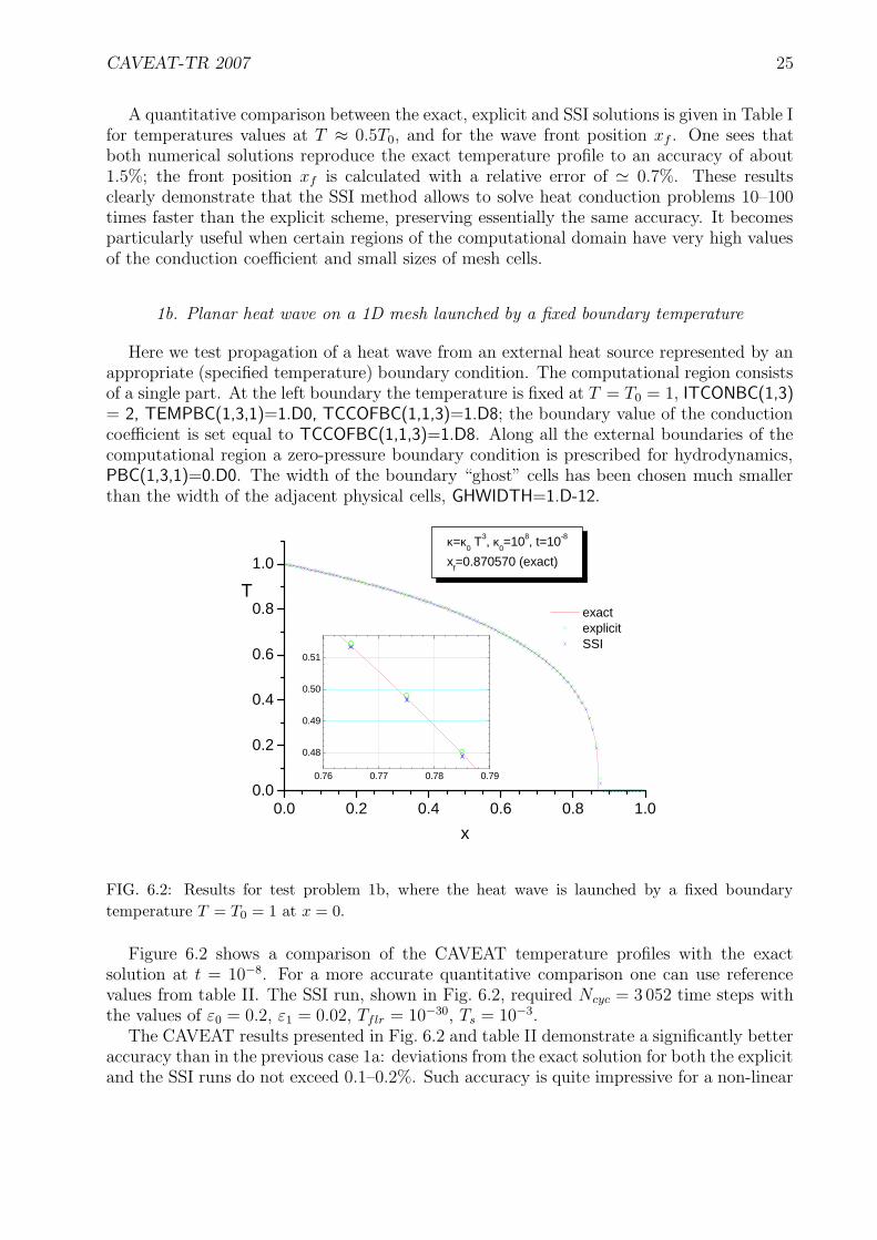
1b. Planar heat wave on a 1D mesh launched by a fixed boundary temperature

Here we test propagation of a heat wave from an external heat source represented by anappropriate (specified temperature) boundary condition. The computational region consistsof a single part. At the left boundary the temperature is fixed at T = T0 = 1, ITCONBC(1,3)= 2, TEMPBC(1,3,1)=1.D0, TCCOFBC(1,1,3)=1.D8; the boundary value of the conductioncoefficient is set equal to TCCOFBC(1,1,3)=1.D8. Along all the external boundaries of thecomputational region a zero-pressure boundary condition is prescribed for hydrodynamics,PBC(1,3,1)=0.D0. The width of the boundary “ghost” cells has been chosen much smallerthan the width of the adjacent physical cells, GHWIDTH=1.D-12.

0.0 0.2 0.4 0.6 0.8 1.00.0

0.2

0.4

0.6

0.8

1.0

0.76 0.77 0.78 0.79

0.48

0.49

0.50

0.51

exact explicit SSI

T

x

κ=κ0 T3, κ

0=108, t=10-8

xf=0.870570 (exact)

FIG. 6.2: Results for test problem 1b, where the heat wave is launched by a fixed boundary

temperature T = T0 = 1 at x = 0.

Figure 6.2 shows a comparison of the CAVEAT temperature profiles with the exactsolution at t = 10−8. For a more accurate quantitative comparison one can use referencevalues from table II. The SSI run, shown in Fig. 6.2, required Ncyc = 3 052 time steps withthe values of ε0 = 0.2, ε1 = 0.02, Tflr = 10−30, Ts = 10−3.

The CAVEAT results presented in Fig. 6.2 and table II demonstrate a significantly betteraccuracy than in the previous case 1a: deviations from the exact solution for both the explicitand the SSI runs do not exceed 0.1–0.2%. Such accuracy is quite impressive for a non-linear

CAVEAT-TR 2007 26

TABLE II: Reference values from the exact, explicit and SSI solutions in test 1b.

reference quantity exact explicit SSI

T at x = 0.775 0.4974 0.4982 0.4968

wave front xf 0.870570 0.8720 ± 0.0005 0.8700 ± 0.0005

wave extending over less than 100 discrete mesh cells. In this way we verify (i) that thespatial part of the SSI algorithm is of sufficiently high accuracy, and (ii) that the boundarycondition for heat conduction is correctly implemented in the code.

1c. Planar heat wave on a skewed 2D mesh launched by a fixed boundary temperature

This example tests propagation of a 1D non-linear planar heat wave on a 2D skewed mesh.The mesh used in this test consists of four quadrangular blocks and is shown in Fig. 6.3. Theheat wave propagates from the bottom boundary of block 3, where the temperature is fixedat T = T0 = 1. The mesh has 50 cells along the y-axis (direction of wave propagation), and25 cells in the perpendicular x direction. Here we test the numerical scheme in the situationwhere the symmetry of the solution (planar) differs significantly from the symmetry of thenumerical grid. The heat conduction coefficient and the equation of state are the same asin test 1b.

0.0 0.1 0.2 0.3 0.4 0.5-0.6

-0.5

-0.4

-0.3

-0.2

-0.1

0.0

0.1

0.2

0.3

0.4

0.5

0.6

block 3

block 2

block 4

x

y

block 1

FIG. 6.3: Skewed 4-block mesh for test problem 1c.

CAVEAT-TR 2007 27

The numerical results are compared with the exact solution in Fig. 6.4 for t = 10−8,where temperature profiles along the x = 0.006 and x = 0.475 lines are plotted. The insertis a blow-up of the region around T = 0.5T0. The SSI run, shown in Fig. 6.4, requiredNcyc = 3 554 time steps with the values of ε0 = 0.2, ε1 = 0.02, Tflr = 10−30, Ts = 10−3.Table III gives temperatures at T ≈ 0.5T0 and the positions of the front for the both profiles.

0.0 0.2 0.4 0.6 0.8 1.00.0

0.2

0.4

0.6

0.8

1.0

0.77 0.78 0.79 0.800.46

0.47

0.48

0.49

0.50

0.51

exact SSI, x=0.006 SSI, x=0.475 explicit, x=0.475

T

y

κ=κ0 T3, κ

0=108, t=10-8

yf=0.870570 (exact)

FIG. 6.4: Results for test problem 1c: a planar heat wave is launched by a fixed boundary tem-

perature T = T0 = 1 at y = 0. Line-out profiles for x = 0.006 and x = 0.475 are plotted.

At x = 0.006 the cells are practically rectangular, and, similar to test 1b, an excellentagreement is observed with the exact solution. For this case only the SSI results are plottedin Fig. 6.4. At x = 0.475 a very close agreement is observed between the SSI and explicitresults, but both differ from the exact solution by about 1.2–1.8%. The observed 1–2%deviation from the exact solution must be caused by the propagation of a planar heat frontthrough skewed quadrangles of the numerical grid.

TABLE III: Reference values from the exact, explicit and SSI solutions in test 1c.

reference quantity exact explicit SSI

x = 0.006

T at y = 0.77 0.5059 – 0.5076

wave front 0.870570 – 0.872 ± 0.0005

x = 0.475

T at y = 0.7755 0.4966 0.5034 0.5028

wave front 0.870570 0.887 ± 0.0005 0.8865 ± 0.0005

With this test, a correct implementation of the inter-block communication scheme hasalso been validated, both along the block edges and at different types of the corner meetingpoints.

CAVEAT-TR 2007 28

6.2. Problem 2: a spherical heat wave from an instantaneous point source

Here we consider a spherically symmetric non-linear heat wave governed by the equation

ρcV∂T

∂t=

1

r2

∂

∂r

(

r2κ∂T

∂r

)

, (6.7)

where the conduction coefficient κ is given by Eq. (6.1). The mass-specific heat capacity cV

and the gas density ρ are supposed to be constant. We assume that at time t = 0 a finiteamount of energy E is instantaneously released in the center at r = 0. The solution to thisproblem is fully analytical and can, for example, be found in Ref. [10, Ch. X]. It has theform

T (r, t) = Tc

(

1 − r2

r2f

)1/n

, (6.8)

where the wave front radius is given by

rf = rf (t) = ξ1

(

κ0t

ρcV

Qn

)1

3n+2

, (6.9)

and the central temperature is

Tc = Tc(t) =

[

nξ21

2(3n + 2)

]1/n

Q2

3n+2

(

ρcV

κ0t

)3

3n+2

. (6.10)

Here the parameter Q is defined as

Q =E

ρcV= 4π

∞∫

0

Tr2dr , (6.11)

and the dimensionless constant

ξ1 =

[

3n + 2

2n−1 n πn

]1

3n+2

[

Γ(

52

+ 1n

)

Γ(

1 + 1n

)

Γ(

32

)

]n

3n+2

(6.12)

is obtained by solving the corresponding eigenvalue problem.For numerical test runs we select a particular case of n = 2 because, on the one hand,

this is already quite close to the physically most interesting case of the Spitzer conductivitywith n = 5/2, while, on the other hand, the parameter ξ1 can be very simply calculated as

ξ1 =27/8

√π

= 1.0347 2826. (6.13)

If, further, we assume Q = 1 and introduce a notation

t =κ0t

ρcV

, (6.14)

CAVEAT-TR 2007 29

0.0 0.2 0.4 0.6 0.8 1.0

0.0

0.2

0.4

0.6

0.8

1.0

block 3

block 2

r

z

block 1

FIG. 6.5: Skewed 3-block mesh for test problem 2.

0.0 0.2 0.4 0.6 0.8 1.00.0

0.1

0.2

0.3

0.4

0.5

0.6

0.00 0.05 0.10 0.15 0.200.55

0.56

0.57

0.58

0.82 0.84 0.86 0.88 0.900.00

0.01

0.02

0.03

0.04

0.05

n=2, t=0.3, ε0=0.2, ε

1=0.02

T

r

exact θ = 0o

θ = 45o

θ = 90o

T2

r

T

r

FIG. 6.6: Temperature profiles for test problem 2: a spherical heat wave is launched at t = 0 by an

instantaneous point source in the center. Three line-outs, corresponding to the polar angle values

θ = 0, 45, and 90, are compared with the exact solution at t = 0.3.

we obtain the following exact values of rf and Tc:

rf = ξ1 t1/8 = 0.890 1567, t = 0.3,

Tc =ξ1

2√

2t−3/8 = 0.574 5937, t = 0.3.

(6.15)

Clearly, by choosing a sufficiently large value of κ0, we can always make the hydrodynamictime scale to be arbitrarily long compared to the thermal time scale t ' ρcV /κ0.

Numerical simulation of the above stated problem was conducted in the cylindrical r, zcoordinates (one of the two principal options for the intrinsic coordinate system in the

CAVEAT-TR 2007 30

TABLE IV: Numerical results for test problem 2 that are to be compared with the following exact

values: Tc = 0.5745937, rf = 0.8901567.

ε0 ε1 Tc rf,z rf,45 rf,r Ncyc

0.01 0.5736 0.887 ± 0.0005 0.896 ± 0.0005 0.8885 ± 0.0005 21 880

0.02 0.5735 0.887 ± 0.0005 0.896 ± 0.0005 0.8885 ± 0.0005 20 080

0.1 0.04 0.5753 0.887 ± 0.0005 0.896 ± 0.0005 0.8885 ± 0.0005 23556

0.05 0.5750 0.887 ± 0.0005 0.896 ± 0.0005 0.8885 ± 0.0005 27 546

0.08 0.5735 0.887 ± 0.0005 0.896 ± 0.0005 0.8885 ± 0.0005 68 701

0.01 0.5731 0.887 ± 0.0005 0.896 ± 0.0005 0.8885 ± 0.0005 17 310

0.02 0.5750 0.887 ± 0.0005 0.896 ± 0.0005 0.8885 ± 0.0005 13 502

0.2 0.03 0.5704 0.887 ± 0.0005 0.896 ± 0.0005 0.8885 ± 0.0005 12 252

0.04 0.5743 0.887 ± 0.0005 0.896 ± 0.0005 0.8885 ± 0.0005 11 819

0.05 0.5698 0.887 ± 0.0005 0.896 ± 0.0005 0.8885 ± 0.0005 11 714

0.08 0.5790 0.887 ± 0.0005 0.896 ± 0.0005 0.8885 ± 0.0005 12 806

CAVEAT code). Since the symmetry of the tested solution is quite different from thesymmetry of the adopted coordinate system, the present test provides a good check forpossible spurious numerical effects that might arise along the z-axis, where the coordinatesingularity occurs. To aggravate the situation, we used a 3-block skewed mesh (see Fig. 6.5)which has no circular symmetry in the r, z plane as well. Because of the rotational symmetryaround the z-axis, our mesh represents one half of a sphere of radius 1.

A progressively increasing cell size was used in the central block 1, so that ∆z11 = ∆r11 =2 × 10−3 for the first cell in the center, and ∆z = ∆r = 2 × 10−2 along, respectively, theθ = 0 (z-axis, r = 0) direction in block 3, and the θ = 90 (radial, z = 0) direction inblock 2. The condition Q = 1 was ensured by setting the initial value of the mass-specificinternal energy in the central cell equal to

e11 =cV

4πV11, (6.16)

where V11 = 12∆r2

11 ∆z is the volume (per steradian of the azimuth angle) of cell (i, j) = (1, 1).Because the volume of the central cell V11 comprises a negligible fraction of 1.2 × 10−8 ofthe total volume of the simulated hemisphere (1/3 per steradian of the azimuth angle),no noticeable effects can be expected from the non-point-like form of the initial energydeposition.

The results of numerical simulations with the SSI algorithm are presented in Fig. 6.6 andtable IV. One of the goals of these simulations was to determine an optimal combination ofthe two SSI accuracy parameters ε0 and ε1, which would ensure a sufficiently good accuracywith not too many time steps Ncyc. From table IV one infers that the values ε0 = 0.2,ε1 = 0.02 are a good combination: the temperature profiles along all three line-outs inFig. 6.6 are described to an accuracy of about 0.2% — which is quite impressive for askewed mesh with a cell size of ∆r = ∆z = 0.02. The optimal ratio between the twoaccuracy parameters appears to be ε1/ε0 = 0.1–0.2. For larger relative values of ε1 slightly

CAVEAT-TR 2007 31

non-monotonic temperature profiles are observed near the center r = z = 0. No spuriousnumerical effects along the rotational z-axis have been detected. A relatively large numberNcyc >∼ 10 000 of time steps in all numerical runs is due to the fact that the temperature

contrast between the initial central value, T11 ≈ 2 × 107, and the “sensitivity” thresholdTs = 10−3 is more than 10 orders of magnitude.

6.3. Problem 3: a planar shock wave with heat conduction

Here we consider a planar shock wave in a medium with non-linear heat conduction. Leta steady-state planar shock propagate with a velocity D along x direction. An ideal-gasequation of state (6.6) is assumed. The gas in front of the shock is at rest and has the initialtemperature T = T0 = 0 and density ρ = ρ0. In the reference frame comoving with theshock front the equations of mass, momentum and energy balance are [10, Ch. VII]

ρu = −ρ0D, (6.17)

p + ρu2 = ρ0D2, (6.18)

ρu

(

γ

γ − 1T +

1

2u2

)

− κdT

dx= −1

2ρ0D

3. (6.19)

After we introduce a new dimensionless variable

η =ρ0

ρ(6.20)

Eqs. (6.17) and (6.18) yield

u = −Dη, (6.21)

T = D2 η(1 − η), (6.22)

whereas the energy equation (6.19) becomes

κdT

dx=

1

2ρ0D

3(1 − η)

(

1 − γ + 1

γ − 1η

)

. (6.23)

Now, the shock structure can be fully resolved in parametric form, with η treated as anindependent parameter. Further on, we consider a specific case of γ = 5/3 and

κ = κ0T2. (6.24)

From Eqs. (6.21)-(6.23) one infers that the unperturbed gas first passes through a thermalprecursor, where η changes continuously from η = η0 = 1 to η = η′

1 = 2/(γ + 1) = 3/4, andthe gas is compressed to ρ = ρ′

1 = ρ0/η′

1 = (4/3)ρ0; the temperature rises from T = T0 = 0to T = T ′

1 = T1 = D2 η′

1(1 − η′

1) = (3/16)D2; see Fig. 6.7. Then the gas passes throughan isothermal (T1 = T ′

1) density jump by a factor ρ1/ρ′

1 = η′

1/η1 = 2/(γ − 1) = 3; the ηparameter jumps from η′

1 = 2/(γ + 1) = 3/4 to η = η1 = (γ − 1)/(γ + 1) = 1/4.By substituting Eqs. (6.22) and (6.24) into Eq. (6.23) and integrating, one obtains

x =κ0

ρ0

(

D

4

)3 [

−16η4 +80

3η3 − 6η2 − 3η − 9

16− 3

4ln

(

2η − 1

2

)]

, (6.25)

CAVEAT-TR 2007 32

where we have assumed x = 0 at the density jump. Equations (6.20)-(6.22) and (6.25) givea full solution in a parametric form for the shock wave structure; in Eqs. (6.22) and (6.25)the parameter η varies within the interval 3/4 ≤ η ≤ 1, where x = 0 and T = T1, and η = 1,where x = xf and T = T0 = 0. For numerical simulations we choose the values κ0 = ρ0 = 1and D = 4; then ρ1 = 4, T1 = 3, p1 = 12, and

xf =53

48− 3

4ln

3

2= 0.8000678. (6.26)

-0.2 0.0 0.2 0.4 0.6 0.8 1.00

1

2

3

4 ρ, exact T, exact ρ, CAVEAT-TR T, CAVEAT-TR

x

T

ρ

FIG. 6.7: Temperature and density profiles for test problem 3: a planar shock front with heat

conduction.

In numerical simulation the shock front was launched by a fixed boundary pressure p1 =12 (rigid piston). Since initially the density jump has no thermal precursor, the shock fronthas to propagate over a certain distance before the steady-state profiles are established.To make this relaxation distance as short as possible, we assign also a fixed boundarytemperature T = T1 = 3 and a conduction coefficient κ = κ0 = 1 at the piston boundary:the resulting heat inflow through the piston surface provides quick replenishment of theenergy that escapes into the precursor region. The computational domain is a simple single-block rectangular region at −10 ≤ x ≤ +1 divided into 300 cells with a progressivelydiminishing length down to ∆x = 0.01 at x = +1. The shock wave is launched at x = −10at time t = 0. By the time t = 2.5 the shock front arrives at x = 0, and Fig. 6.7 showsthe density and temperature profiles at this moment. More precisely, the profiles are shiftedby ∆x = +0.035 to place the density jump at x = 0 exactly (this small discrepancy in thedistance traveled must be due to the non-equilibrium initial shock front structure). ThisCAVEAT run required 17 333 time steps with ε0 = 0.2, ε1 = 0.02, and Ts = 10−3. In Fig. 6.7one sees that the exact solution is reasonably well reproduced, with a typical error for thetemperature profile at the front end of the precursor being ' 2%.

CAVEAT-TR 2007 33

APPENDIX A: CAVEAT INTERPOLATION SCHEMES

1. Vertex temperatures

The original CAVEAT version contains an explicit algorithm for heat conduction, which,in addition to cell-centered temperatures T , uses vertex-centered values Tv to evaluate theface-centered temperature gradients. The values of Tv are obtained by interpolation fromthe surrounding four cell-centered values of T . We take this scheme over to CAVEAT-TRwithout changes.

Besides the mesh geometry, the CAVEAT algorithm for evaluating Tv uses also cell-centered values of the conduction coefficient κ to calculate the corresponding interpolationcoefficients. Being quite appropriate for heat conduction proper, this is questionable for

radiation transport. To illustrate the idea, first consider the simpler 1D case.

a. 1D interpolation

Assume that the temperature values T and T+ are associated with the cell centers xc andxc+, respectively; see Fig. A.1. Then, if we want to evaluate the temperature Tv at a meshnode xv (xc ≤ xv ≤ xc+), the simplest algorithm would be based on the assumption of acontinuous gradient ∇T at point xv:

Tv − T

xv − xc=

T+ − Tv

xc+ − xv, (A.1)

which leads us to the expression

Tv =(xc+ − xv) T + (xv − xc) T+

xc+ − xv + xv − xc. (A.2)

T κ, T

xc

xv

xc+

x

Tv

κ+, T

+

FIG. A.1: 1D illustration of the temperature interpolation algorithm.

However, in many cases, when the conduction coefficient κ is either a strong function oftemperature or simply discontinuous, it will be more physical to assume that the flux κ∇Tis continuous rather than ∇T . In our 1D case this leads to

κTv − T

xv − xc

= κ+T+ − Tv

xc+ − xv

(A.3)

CAVEAT-TR 2007 34

instead of (A.2); from Eq. (A.3) we calculate

Tv =κ(xc+ − xv) T + κ+(xv − xc) T+

κ(xc+ − xv) + κ+(xv − xc). (A.4)

An obvious generalization of Eq. (A.4) to a multidimensional case from a “normal” (con-tinuous gradient) interpolation scheme

Tv =

∑

α µα Tα∑

α µα(A.5)

will be

Tv =

∑

α καµα Tα∑

α καµα. (A.6)

This is exactly the scheme adopted in CAVEAT to evaluate the vertex temperatures Tv.

b. 2D interpolation

In CAVEAT the 2D interpolation for calculating the vertex temperatures is based on alocal bilinear interpolation on a mathematical ξ, η plane. Let us assume that a rectangle,made up by four cell centers ~xcα surrounding mesh vertex (i, j), is mapped onto a square−1 ≤ ξ ≤ +1, −1 ≤ η ≤ +1 on a mathematical plane of “natural coordinates” ξ and η (seeFig. A.2). Then an obvious bilinear interpolation

T (ξ, η) = T(+1,+1)1

4(1 + ξ)(1 + η) + T(−1,+1)

1

4(1 − ξ)(1 + η) +

T(−1,−1)1

4(1 − ξ)(1 − η) + T(+1,−1)

1

4(1 + ξ)(1 − η) (A.7)

can be written for any function T (x, y) (in this subsection we use the notation x1 = x,x2 = y), based on four values T(±1,±1) at the corresponding corners ξ = ±1, η = ±1 of the“natural” square.

xc3

x

vertex (i,j)

(+1,+1)xc2

xc1

xc4

ξ

η

+1-1

+1

-1

(-1,+1)

(+1,-1)(-1,-1)

FIG. A.2: 2D mapping of a rectangular cell (i, j) in physical space onto a “natural” square in

mathematical ξ, η space.

It is assumed that the mapping of physical coordinates x, y onto the ξ, η plane is performedby the same bilinear interpolation (A.7) with T (ξ, η) replaced by either x(ξ, η) or y(ξ, η).

CAVEAT-TR 2007 35

Then the values of ξ and η, corresponding to the vertex point ~xij = ~x = x; y, can befound from the following system of equations,

x =1

4(xc1 + xc2 + xc3 + xc4) +

1

4(xc1 − xc2 − xc3 + xc4) ξ +

1

4(xc1 + xc2 − xc3 − xc4) η +

1

4(xc1 − xc2 + xc3 − xc4) ξη, (A.8)

y =1

4(yc1 + yc2 + yc3 + yc4) +

1

4(yc1 − yc2 − yc3 + yc4) ξ +

1

4(yc1 + yc2 − yc3 − yc4) η +

1

4(yc1 − yc2 + yc3 − yc4) ξη, (A.9)

which is easily reduced to a quadratic equation. Here we used the CAVEAT convention fornumbering the cell centers around vertex (i, j): center 1 is the center of cell (i, j), center 2is the center of cell (i − 1, j), . . . (see Fig. A.2).

Finally, taking into account correction for possible strong variations of the conductioncoefficient κ, we obtain the following interpolation formula for the vertex temperature Tv:

Tv =κ1T1 (1 + ξ)(1 + η) + κ2T2 (1 − ξ)(1 + η) + κ3T3 (1 − ξ)(1 − η) + κ4T4 (1 + ξ)(1 − η)

κ1 (1 + ξ)(1 + η) + κ2 (1 − ξ)(1 + η) + κ3 (1 − ξ)(1 − η) + κ4 (1 + ξ)(1 − η).

(A.10)

2. Face-centered heat flux

Consider a single mesh cell (i, j), as it is shown in Figs. 3.1 and 5.1. For brevity, inthis section we omit the indices (i, j) for all quantities. To implement the SSI algorithm forheat conduction, we need explicit expressions for the total heat fluxes H1 and H2 [erg s−1]through the two faces 1 and 2 of this cell, which emerge from the vertex (i, j). Here wecombine the formulae for both faces by using universal vector notations.

Let~λv = ~x+ − ~x, ~λc = ~xc − ~xc− (A.11)

be the two vectors connecting, respectively, the two vertices along the considered face m,

and the cell centers across this same face (see Fig. A.3). Vector ~λv starts at vertex (i, j);

vector ~λc ends at cell center (i, j). Let further T , T−, Tv, Tv+ be, respectively, the values oftemperature at the relevant cell centers ~xc, ~xc−, and the relevant vertices ~x, ~x+; see Fig. A.3.

To calculate the fluxH = −κf

[

(∇T )f · ~nf

]

|~λv|Rf , (A.12)

given by Eq. (5.2), we have to evaluate the face-centered conduction coefficient κf , and theface-centered temperature gradient

~g = (∇T )f . (A.13)

CAVEAT-TR 2007 36

Tv+

xc–

TT

–

Tv+

Tv

T–

T

Tv

x+

xc

x

x

xc

xc–

x+

λv

λv

λc

λc

face 1 face 2

(i,j)

(i,j)

(i,j-1)

(i+1,j)

(i,j)

(i,j+1)

(i-1,j)

(i,j)

FIG. A.3: Vector scheme for temperature gradient evaluation.

The components of the inward-oriented unit normal ~nf (as defined in Fig. 3.1) are given by

~nf = −λv,2; λv,1ωm

|~λv|, face 1,

~nf = λv,2; −λv,1ωm

|~λv|, face 2,

(A.14)

where

ωm =

+1, right-handed mesh,

−1, left-handed mesh.(A.15)

The face-centered radius Rf is given by

Rf =1

2(R + R+), (A.16)

where R and R+ are, respectively, the radii of vertices ~x and ~x+.The gradient ~g is calculated by solving the system of two linear equations

~g · ~λv = Tv+ − Tv,

~g · ~λc = T − T−,(A.17)

the mathematical meaning of which is clear from Fig. A.3. The solution of (A.17) is givenby

g1 = J−1 [λc,2(Tv+ − Tv) − λv,2(T − T−)] ,

−g2 = J−1 [λc,1(Tv+ − Tv) − λv,1(T − T−)] ,

(A.18)

where

J = ~λv ⊗ ~λc = λv,1λc,2 − λv,2λc,1 =

+|J |ωm, face 1,

−|J |ωm, face 2,(A.19)

and symbol ⊗ denotes a vector product.

CAVEAT-TR 2007 37

Finally, after we substitute Eqs. (A.14) and (A.18) into Eq. (A.12), we obtain

H =κfRf

|J |[(

~λv · ~λc

)

(Tv+ − Tv) − |~λv|2(T − T−)]

. (A.20)

This is the basic expression which enables us to calculate both the explicit fluxes Hijm andthe coefficients aijm, bijm required in the SSI method (see section 4 above).

3. Face-centered conduction coefficient

In the original CAVEAT version the face-centered conduction coefficient κf is evaluatedas an average of the two adjoining cell-centered values,

κf,ij1 = κij

A−

∆,ij1

A−

∆,ij1 + A+∆,ij1

+ κi,j−1

A+∆,ij1

A−

∆,ij1 + A+∆,ij1

, (A.21)

κf,ij2 = κij

A−

∆,ij2

A−

∆,ij2 + A+∆,ij2

+ κi−1,j

A+∆,ij2

A−

∆,ij2 + A+∆,ij2

. (A.22)

The corresponding weights are proportional to the areas A±

∆,ijm of the two adjacent triangles— i.e. to normal distances from the adjacent cell centers to the face (i, j, m); see Fig. 5.3.The idea is that if, for example, a cell center (i, j) lies very close to face (i, j, m) (i.e.A+

∆,ijm → 0), then we must have κf,ijm = κij. Note that area values A±

∆,ijm, calculatedas vector products, can be negative. An additional constraint is imposed that the weightcoefficients in Eqs. (A.21) and (A.22) should lie between 0 and 1.

[1] P. Woodward and Ph.Colella, J. Comp. Physics 54 (1984) 115.

[2] P. Woodward and Ph.Colella, J. Comp. Physics 54 (1984) 174.

[3] R.B. Pember, R.W. Anderson, Comparison of Direct Eulerian Godunov and Lagrange Plus

Remap, Artificial Viscosity Schemes, UCRL-JC-143206 (Livermore, 2001).

[4] R. Ramis and J. Meyer-ter-Vehn, MPQ report 174, 1992; http://server.faia.upm.es/multi.

[5] M.M. Basko, J. Maruhn, and T. Schlegel, Phys. Plasmas, 9 (2002) 1348.

[6] M.M. Basko, T. Schlegel, and J. Maruhn, Phys. Plasmas, 11 (2004) 1577.

[7] F. L. Addessio, J. R. Baumgardner, J. K. Dukowicz, N. L. Johnson, B. A. Kashiwa,

R. M. Rauenzahn, and C. Zemach, CAVEAT: A Computer Code for Fluid Dynamics Problems

With Large Distortion and Internal Slip, LA-10613-MS, Rev. 1, UC-905 (Los Alamos, 1992).

[8] A.I. Shestakov, J.L. Milovich, and M.K. Prasad, J. Comp. Physics 170 (2001) 81.

[9] E. Livne and A. Glasner, J. Comp. Physics 58 (1985) 59.

[10] Ya. B. Zel’dovich and Yu. P. Raizer, Physics of Shock-Waves and High-Temperature Hydro-

dynamic Phenomena. Vol. II. (Academic Press, New York, 1967.)