2010 ka mun ho all rights reserved
TRANSCRIPT

©2010
Ka Mun Ho
ALL RIGHTS RESERVED
AUTOMATIC RECOGNITION AND DEMODULATION OF DIGITALLY
MODULATED COMMUNICATIONS SIGNALS USING WAVELET-DOMAIN
SIGNATURES
by
KA MUN HO
A Dissertation submitted to the
Graduate School-New Brunswick
Rutgers, The State University of New Jersey
in partial fulfillment of the requirements
for the degree of
Doctor of Philosophy
Graduate Program in Electrical and Computer Engineering
written under the direction of
Professor David G. Daut
and approved by
________________________
________________________
________________________
________________________
________________________
New Brunswick, New Jersey
January, 2010
ii
ABSTRACT OF THE DISSERTATION
Automatic Recognition and Demodulation of Digitally Modulated Communications
Signals Using Wavelet-Domain Signatures
By KA MUN HO
Dissertation Director: Professor David G. Daut
Abstract – Wavelet transform-based methodologies for both Automatic Modulation
Recognition (AMR) and Demodulation of digitally modulated communications signals
can be utilized in an enabling platform for the implementation of a new class of
communications systems. In particular, such techniques could enable the development of
agile radio transceivers for use in both commercial and military applications. Such radio
transceivers would have the ability to transmit and receive signals using many different
modulation schemes while employing a common receiver architecture based on a single
demodulator.
In this dissertation, the development of AMR and Demodulation techniques are based on
the relatively new mathematical theory of Wavelet Transforms (WTs). Information-
bearing signals acquired by communications receivers are transformed into the wavelet-
domain using the Continuous Wavelet Transform (CWT) and then applied to signal
processing algorithms that also use the CWT in conjunction with pattern recognition
techniques. In particular, the method of template-matching is used for both the AMR and
Demodulation processes. Signal templates characterizing various modulated signals are

iii
used for both processes. The signal templates are determined based on the signal features
present in the fractal patterns of their corresponding scalograms for specific modulation
schemes as they appear in the wavelet-domain. The algorithms developed in this work are
capable of both classifying the method of modulation used in the acquired signal, as well
as subsequently automatically demodulating the signal to recover the message.
The classes of digitally modulated signals considered in this work include variants of the
Amplitude-, Frequency-, Phase-Shift Keying modulation families, i.e., ASK, FSK, and
PSK, respectively, and multiple-level Quadrature Amplitude Modulation (M-ary QAM)
families. The AMR and Demodulation performances are evaluated in the presence of
Additive White Gaussian Noise (AWGN) over a wide range of Signal-to-Noise Ratio
(SNR) values. Through extensive Monte Carlo computer simulations it is determined
that the average correct classification rates using wavelet-based AMR for PSK, ASK, and
QAM are over 98%, and over 90% for FSK signals, all at an SNR of 0 dB. The Bit Error
Rate (BER) performance obtained using wavelet-based Demodulation is at least one
order of magnitude better than the matched filter-based BER performance realized for the
modulation schemes considered.
iv
Acknowledgement
First, I would like to express my gratitude to my advisor Professor David G. Daut
for his guidance and support throughout my Ph.D. studies at Rutgers, the State University
of New Jersey. I have benefited from his knowledge and technical insight on digital
communications. Most importantly, I have adapted my research skills, and style on
technical presentation and writing technical documents from Prof. Daut.
I would like to express my gratitude to my Ph.D. committee members, Prof.
Zoran Gajic, Prof. Sophocles Orfanidis, and Prof. Lawrence Rabiner. I would also like to
thank Prof. Anant Madabushi for serving as the dissertation external committee member.
Also, I have to thank Prof. Sigrid R. McAfee for her guidance on pursuing a Ph.D. degree
in Electrical Engineering, and the way of solving engineering problems during my early
years in graduate school.
I would like to extend my thanks to my colleague, Mr. Canute Vaz, for his helpful
technical discussions on different topics in Electrical Engineering. I would also like to
thank all of my friends for their accompaniment and providing me for the much needed
distractions outside work.
Finally, I would like to thank my mother for her encouragement, love and
friendship. She has made many sacrifices so as to provide me with the best education in
the United States.

v
Dedication
To my mother
vi
Table of Contents
Abstract of the Dissertation ...................................................................................... ii
Acknowledgement ..................................................................................................... iv
Dedication .................................................................................................................. v
List of Tables ............................................................................................................. x
List of Illustrations ..................................................................................................... xii
1. Introduction ....................................................................................................... 1
1.1 Motivation ................................................................................................... 2
1.2 Objective ..................................................................................................... 8
1.3 Major Contributions of the Dissertation ..................................................... 12
1.4 Organization of the Dissertation ................................................................ 12
2. Literature Survey .............................................................................................. 15
2.1 Automatic Modulation Recognition Techniques ........................................ 15
2.1.1 Techniques Based on the Decision-Theoretic Approach ................... 16
2.1.2 Techniques Based on the Pattern-Recognition Approach ................. 18
2.1.3 The Use of Artificial Neural Networks and Support Vector
Machines for Modulation Recognition ..............................................
19
2.1.4 Wavelet Transform-Based Techniques ............................................. 21
2.2 Techniques for Demodulation of Digital Data ............................................ 23
3. Mathematical Preliminaries ............................................................................. 25
3.1 An Overview of the Wavelet Transform ....................................................... 25
3.1.1 Review of the Continuous Wavelet Transform .................................... 27
3.1.2 Review of Multiresolution Analysis and the Discrete Wavelet
vii
Transform .............................................................................................. 31
3.2 Digital Communications Signal Models ........................................................ 33
3.3 Wavelet-Domain Cross-Correlation Operation ............................................. 34
4. Setup of the Automatic Modulation Recognition Process ............................. 37
4.1 Template Selection for the Wavelet-Domain Automatic Modulation
Recognition Process .......................................................................................
38
4.2 Mathematical Models of the Templates for Wavelet-Domain Signatures ..... 49
4.3 Determining the Length of the Templates for Wavelet-Domain Signatures . 52
4.4 Selection of Wavelets to be Used for Automatic Modulation Recognition ... 57
4.4.1 Selection of Wavelets Using Unique Features Templates .................... 58
4.4.2 Selection of Wavelets Using Common Features Templates ................. 65
4.5 Discussion of Methodologies ......................................................................... 68
5. Automatic Modulation Recognition Process Using Unique Features
Templates ..........................................................................................................
72
5.1 Development of the Automatic Modulation Recognition Process Using
Unique Features Templates ............................................................................
72
5.2 Simulation Experiment and Results ............................................................... 80
5.3 Comparison of Results ................................................................................... 82
5.4 Conclusions .................................................................................................... 85
6. Automatic Modulation Recognition Process Using Common Features
Templates ..........................................................................................................
88
6.1 Development of the Automatic Modulation Recognition Process Using
Common Features Templates ........................................................................
88

viii
6.2 Algorithm for the Automatic Modulation Recognition Process .................... 104
6.2.1 Procedure for Decision Block 1 ............................................................ 107
6.2.2 Procedure for Decision Block 2 ............................................................ 110
6.2.3 Procedure for Decision Block 3 ............................................................ 112
6.2.4 Procedures for Other Decision Blocks .................................................. 113
6.2.4.1 ASK and FSK Classifier Procedure .......................................... 113
6.2.4.2 PSK and QAM Classifier Procedure......................................... 116
6.3 Simulation Experiment and Results ............................................................... 126
6.4 Comparison of Results ................................................................................... 133
6.5 Conclusions .................................................................................................... 137
7. Techniques for Demodulation Using Wavelet-Domain Templates .............. 139
7.1 Demodulation Using Unique Features Templates ......................................... 140
7.2 Demodulation Using Common Features Templates ...................................... 145
7.2.1 Demodulation Techniques for Phase Shift Keyed Signals ................ 145
7.2.2 Demodulation Techniques for Frequency Shift Keyed Signals ......... 150
7.2.3 Demodulation Techniques for Amplitude Shift Keyed Signals ........ 153
7.2.4 Demodulation Techniques for Quadrature Amplitude Modulated
Signals ................................................................................................
156
7.3 Simulation Experiments and Results ............................................................. 162
7.4 Discussion of Results ..................................................................................... 170
8. Summary and Conclusions............................................................................... 176
8.1 Summary ........................................................................................................ 176
8.2 Contributions of the Dissertation ................................................................... 177
ix
8.3 Applications ................................................................................................... 178
8.4 Suggestions for Future Work ......................................................................... 179
8.5 Conclusions .................................................................................................... 181
References 183
Appendix A: Algorithm for Demodulating a 64-QAM Signal .................................. 190
Appendix B: Algorithm for Demodulating a 256-QAM Signal ................................ 193
Appendix C: Constants Used for the Common Features Templates for M-ary
QAM Signals ........................................................................................
199
Curriculum Vitae ....................................................................................................... 200

x
Lists of Tables
Table 1.1 MPSK modulation schemes and major applications ................................. 10
Table 1.2 M-ary QAM modulation schemes and major applications ........................ 11
Table 4.1 Number of unique features templates needed for different modulation
schemes .....................................................................................................
69
Table 5.1 Rates of correct classification for SNR = 10 dB [85] ................................ 81
Table 5.2 Rates of correct classification for SNR = 5 dB [85] .................................. 81
Table 5.3 Rates of correct classification for SNR = 0 dB [85] .................................. 81
Table 5.4 Rates of correct classification for SNR = -5 dB [85] ................................. 82
Table 5.5 Survey of the literature for BASK classification [85] ............................... 83
Table 5.6 Survey of the literature for BFSK classification [85] ................................ 83
Table 5.7 Survey of the literature for BPSK classification [85] ................................ 84
Table 5.8 Rates of correct classification for different baseband symbol sequence
lengths using BPSK signals .......................................................................
86
Table 6.1 Cross-correlation values of Template 1 and a sinusoidal function with
different phase shifts .................................................................................
92
Table 6.2 Cross-correlation values of Template 2 and a sinusoidal function with
different phase shifts .................................................................................
93
Table 6.3 Identification of signal space quadrant using the cross-correlation
results of Template 1 and Template 2 .......................................................
93
Table 6.4 Attributes of WD cross-correlation values from test cases with
Template 1 .................................................................................................
102
Table 6.5 Attributes of WD cross-correlation values from test cases with

xi
Template 2 ................................................................................................. 103
Table 6.6 Attributes of WD cross-correlation values from test cases with
Template 3 ...............................................................................................
103
Table 6.7 Two groups of data identified from Template 1 using dynamic range ...... 107
Table 6.8 Two groups of data identified from Template 1 using multi-level ............ 107
Table 6.9 Criteria used in Decision Block 1 .............................................................. 108
Table 6.10 Dynamic range of the cross-correlation data with Template 2 ................ 111
Table 6.11 Rates of correct classification for WD AMR process; SNR = 10 dB ...... 128
Table 6.12 Rates of correct classification for WD AMR process; SNR = 5 dB ........ 129
Table 6.13 Rates of correct classification for WD AMR process; SNR = 0 dB ........ 130
Table 6.14 Rates of correct classification for WD AMR process; SNR = -3 dB ...... 131
Table 6.15 Rates of correct classification for WD AMR process; SNR = -5 dB ...... 132
Table 6.16 Non-wavelet transform-based AMR methods ......................................... 135
Table 6.17 Wavelet transform-based AMR methods ................................................ 136
Table 6.18 AMR classification rates obtained in this research work ........................ 137
Table 7.1 BER results for WD Demodulation process using unique features
templates ....................................................................................................
144
Table C1 Constants used for the Common Features Templates for M-ary QAM
Signals .......................................................................................................
199
xii
List of Illustrations
Fig. 1.1. Overall system-level description of a radio receiver [1] ............................. 3
Fig. 1.2. Typical contemporary radio transceiver system [1] .................................... 4
Fig. 1.3. A basic system block diagram of an agile radio receiver ............................ 5
Fig. 1.4. System-level block diagram of an agile radio transceiver based on the
Wavelet Platform [2] ....................................................................................
7
Fig. 2.1. DWT of different modulated signals [54] ................................................... 22
Fig. 3.1. (Top) A time-domain sinusoidal signal, (Bottom) The corresponding WD
scalogram of the sinusoidal signal ................................................................
28
Fig. 3.2. A three-level filter bank illustrative of the MRA process ........................... 31
Fig. 4.1. Time-domain BASK signal with transitions contained within the box ....... 39
Fig. 4.2. Time-domain BFSK signal with transitions contained within the box ....... 39
Fig. 4.3. Time-domain BPSK signal with transitions contained within the box ....... 39
Fig. 4.4. Wavelet-domain scalogram of the BASK signal ......................................... 40
Fig. 4.5. Wavelet-domain scalogram of the BFSK signal ......................................... 40
Fig. 4.6. Wavelet-domain scalogram of the BPSK signal ......................................... 40
Fig. 4.7. Time-domain BASK signal with common features contained within the
boxes .............................................................................................................
42
Fig. 4.8. Time-domain BFSK signal with common features contained within the
boxes .............................................................................................................
42
Fig. 4.9. Time-domain BPSK signal with common features contained within the
boxes .............................................................................................................
42
Fig. 4.10. Wavelet-domain scalogram of the BASK signal with the common
xiii
features templates highlighted ................................................................... 44
Fig. 4.11. Wavelet-domain scalogram of the BFSK signal with the common
features templates highlighted ...................................................................
44
Fig. 4.12. Wavelet-domain scalogram of the BPSK signal with the common
features templates highlighted ...................................................................
44
Fig. 4.13. (a-q) WD scalograms of the unique features corresponding to all sixteen
symbol transitions in a QPSK signal .........................................................
46
Fig. 4.14. (a) Time-domain BPSK signal, (b) WD scalogram for the BPSK signal,
(c) Time-domain QPSK signal, and (d) WD scalogram of the QPSK
signal .........................................................................................................
47
Fig. 4.15. (a) Time domain 4-FSK signal, and (b) WD scalogram of the 4-FSK
signal .........................................................................................................
48
Fig. 4.16. Illustration of time-domain unique features templates .............................. 50
Fig. 4.17. Illustration of common features templates at different locations within a
symbol .......................................................................................................
51
Fig. 4.18. Illustration of the sliding cross-correlation process between a template
and a communications signal ....................................................................
53
Fig. 4.19. Graphical representation of the cross-correlation operation using
different template lengths ..........................................................................
54
Fig. 4.20. Scalogram of a BPSK test signal ............................................................... 55
Fig. 4.21. WD unique features Template 1 with length of (a) 128 samples, (b) 64
samples, and (c) 32 samples ......................................................................
55
Fig. 4.22. Cross-correlation results using a unique features template that is 32
xiv
samples in length ....................................................................................... 56
Fig. 4.23. Cross-correlation results using a unique features template that is 64
samples in length .......................................................................................
56
Fig. 4.24. Cross-correlation results using a unique features template that is 128
samples in length .......................................................................................
56
Fig. 4.25. Cross-correlation values arranged in sub-matrices within the matrix
image .........................................................................................................
60
Fig. 4.26. An example of the construction of the sub-matrices ................................. 61
Fig. 4.27. Matrix image with a threshold value Δ= 0 ............................................... 62
Fig. 4.28. Matrix image with a threshold value of Δ = 1 .......................................... 63
Fig. 4.29. Matrix image with a threshold value of Δ = 2 .......................................... 64
Fig. 4.30. Matrix image with a threshold value of Δ = 2.5 ....................................... 65
Fig. 4.31. Common feature templates highlighted in boxes in (a) BASK signal, (b)
BFSK signal, and (c) BPSK signal ............................................................
66
Fig. 4.32. Matrix image based on the common features templates, with a threshold
value of Δ = 1 ...........................................................................................
68
Fig. 5.1. Unique features templates for BASK signal (a-b) in time-domain, (c-d)
in wavelet-domain .......................................................................................
73
Fig. 5.2. Unique features templates for BFSK signal (a-b) in time-domain, (c-d) in
wavelet-domain ...........................................................................................
74
Fig. 5.3. Unique features templates for BPSK signal (a-b) in time-domain, (c-d) in
wavelet-domain ...........................................................................................
74
Fig. 5.4. Example of a “time-and-merged” operation in the WD AMR process ....... 76
xv
Fig. 5.5. Block diagram of the WD AMR process using unique features templates . 77
Fig. 5.6. Example of WD AMR process using unique features templates ................ 79
Fig. 6.1. Signal space representation of the three common features templates ......... 90
Fig. 6.2. The three common features templates used for the AMR process .............. 91
Fig. 6.3. Results of cross-correlation between BASK test signals and the common
features templates ........................................................................................
94
Fig. 6.4. Results of cross-correlation between 4-ASK test signals and the common
features templates ........................................................................................
95
Fig. 6.5. Results of cross-correlation between BFSK test signals and the common
features templates ........................................................................................
95
Fig. 6.6. Results of cross-correlation between 4-FSK test signals and the common
features templates ........................................................................................
96
Fig. 6.7. Results of cross-correlation between BPSK test signals and the common
features templates ........................................................................................
97
Fig. 6.8. Results of cross-correlation between QPSK test signals and the common
features templates ........................................................................................
98
Fig. 6.9. Results of cross-correlation between 8-PSK test signals and the common
features templates ........................................................................................
98
Fig. 6.10. Results of cross-correlation between the 4-QAM ( 4π -QPSK) test signal
and the common features templates ................................................................
99
Fig. 6.11. Results of cross-correlation between 16-QAM test signals and the
common features templates .......................................................................
100
Fig. 6.12. Results of cross-correlation between 64-QAM test signals and the

xvi
common features templates ....................................................................... 101
Fig. 6.13. Results of cross-correlation between 256-QAM test signals and the
common features templates .......................................................................
101
Fig. 6.14. Block diagram of the WD AMR process using common features
templates ....................................................................................................
106
Fig. 6.15. Flowchart of the procedure for Decision Block 1 ..................................... 110
Fig. 6.16. Flowchart of the procedure for Decision Block 2 ..................................... 111
Fig. 6.17. Flowchart of the procedure for Decision Block 3 ..................................... 112
Fig. 6.18. Additional common features templates used in the ASK and FSK
Classifier Procedure ..................................................................................
114
Fig. 6.19. System block diagram implementing the ASK and FSK Classifier
Procedure for Group 1 signals ...................................................................
115
Fig. 6.20. Signal constellations of M-ary QAM signals ............................................ 116
Fig. 6.21. Signal space representation of Group 2 signals in Quadrant I .................. 117
Fig. 6.22. Introduction of new I and Q axes in Quadrant I ........................................ 118
Fig. 6.23. Location of the new features template ....................................................... 120
Fig. 6.24. Location of the new features templates used for classifying QAM
signals ........................................................................................................
121
Fig. 6.25. The signal space depicting the new templates with special locations
indicated in Quadrant I ..............................................................................
123
Fig. 6.26. System block diagram implementing the PSK and QAM Classifier
Procedure for Group 2 signals in Quadrant I ............................................
125
Fig. 7.1. System-level block diagram for the WD Demodulation process ................ 141

xvii
Fig. 7.2. Example of WD Demodulation process using Templates 1 and 2 .............. 142
Fig. 7.3. Signal constellations for M-ary PSK signals ............................................... 146
Fig. 7.4. System block diagram for the BPSK demodulator in the WD .................... 147
Fig. 7.5. System block diagram for the QPSK demodulator in the WD .................... 148
Fig. 7.6. System block diagram for the 8-PSK demodulator in the WD ................... 150
Fig. 7.7. System block diagram for the BFSK demodulator in the WD .................... 151
Fig. 7.8. System block diagram for the 4-FSK demodulator in the WD ................... 153
Fig. 7.9. System block diagram for the BASK demodulator in the WD .................... 154
Fig. 7.10 Example plot of the WD cross-correlation of a 4-ASK signal with
Template 1. .................................................................................................
155
Fig. 7.11. System block diagram for the 4-ASK demodulator in the WD ................. 156
Fig. 7.12. Quadrant I of the 16-QAM signal constellation ........................................ 157
Fig. 7.13. Quadrant I of the 64-QAM signal constellation ........................................ 158
Fig. 7.14. Quadrant I of the 256-QAM signal constellation ...................................... 158
Fig. 7.15. System block diagram for the 4-QAM demodulator in the WD ............... 161
Fig. 7.16. WD demodulation performance for BPSK ................................................ 163
Fig. 7.17. WD demodulation performance for QPSK ................................................ 164
Fig. 7.18. WD demodulation performance for 8-PSK ............................................... 164
Fig. 7.19. WD demodulation performance for BASK ............................................... 165
Fig. 7.20. WD demodulation performance for 4-ASK .............................................. 165
Fig. 7.21. WD demodulation performance for BFSK ................................................ 166
Fig. 7.22. WD demodulation performance for 4-FSK ............................................... 166
Fig. 7.23. WD demodulation performance for 4-QAM ( 4π -QPSK) ....................... 167

xviii
Fig. 7.24. WD demodulation performance for 16-QAM ........................................... 167
Fig. 7.25. WD demodulation performance for 64-QAM ........................................... 168
Fig. 7.26. WD demodulation performance for 256-QAM ......................................... 168
Fig. 7.27. (Top) BFSK signal at 10 dB SNR, (bottom) 12-level wavelet-domain
decomposition using the Reverse Biorthogonal 1.3 wavelet ....................
174
Fig. 7.28. (Top) BFSK signal without noise, (bottom) 12-level wavelet-domain
decomposition using the Reverse Biorthogonal 1.3 wavelet ....................
175
Fig. A1. Quadrant I of the 64-QAM signal constellation .......................................... 190
1
Chapter 1
Introduction
A distinctive trend in the development of communications systems, for use in both
commercial and military applications, is that the operating characteristics of such systems
are becoming increasing stringent. In particular, systems are required to have the features
of high reliability, portability, security, and also simultaneously consume ever smaller
amounts of power. Communications engineers are required to design systems based on
existing and emerging communications protocols and standards that cater to the different
needs of customers while meeting these challenging requirements.
Typical contemporary communications systems are developed based on a wide range of
wireless protocols and standards. For example, cellular phone systems may employ either
Code Division Multiple Access (CDMA) or the Global System for Mobile
communications (GSM), and personal wireless networks may follow either the IEEE
802.11 family of standards or the newly developed technology of Worldwide
Interoperability for Microwave Access (WiMAX). With the variety of standards currently
in use, there exist entire families of communications systems that are tailored specifically
to each standard.
With consumers starting to use multiple communications devices, either in mobile, or in
fixed locations, there is an implicit drawback to the current state of the art. The drawback
is the lack of interoperability between such devices. In order to overcome this deficiency,
a new paradigm is needed for the development of future communications systems that
has a focus on the interoperability between different standards.
2
Such futuristic communications systems can be described as agile radio systems. Ideally,
an agile radio should have the flexibility to transmit signals at different carrier
frequencies and use different modulation schemes. In addition, the system should be able
to correctly classify and appropriately demodulate signals in real-time. Automation of
these functions is at the core of the agile nature of such radio systems.
With the use of the mathematical theory of Wavelet Transforms (WTs) the development
of agile radio transceiver systems is possible. The development of such a system is the
primary motivation of this dissertation with the focus on two of the core features of an
agile transceiver, namely Automatic Modulation Recognition (AMR) and the subsequent
Automatic Demodulation of communications signals.
Therefore, the focal points of this dissertation are:
1. The invention of WT-based techniques for the AMR of a select group of digitally
modulated communications signals.
2. The invention of WT-based techniques for the Automatic Demodulation of
digitally modulated communications signals subsequent to the AMR process.
1.1 Motivation
A typical contemporary communications receiver can be implemented by the means of
three major sub-systems, as illustrated in Fig. 1.1.

3
Fig. 1.1. Overall system-level description of a radio receiver [1].
1. Radio Frequency (RF) front-end: The RF front-end performs the down-
conversion of the passband signal to an intermediate frequency for the ease of
subsequent processing. It is composed of analog electronic sub-systems, such as
mixer, local oscillators, band-pass filters, variable gain amplifiers and antennas.
2. Mixed-signal stage: This stage converts the downconverted signal output by the
RF front-end to a digitized form. This stage is absent in analog receivers. The
Analog-to-Digital Converter (ADC), in Fig. 1.1, converts the analog received
signal into digitized form.
3. Demodulation and baseband processing units: The desired baseband data are
recovered by a signal-specific demodulator, and any decoding of the recovered
data is handled by a baseband processor.
Radio transmitters also use similar signal processing strategies as those in the receiver,
except in reverse. First, baseband data are encoded, if needed, and the data are then used
to modulate a carrier signal at an intermediate frequency. The modulated signal is then
upconverted to the RF passband and transmitted.
A more detailed depiction of a modern radio transceiver system is provided in Fig. 1.2.

4
Baseband Processor
Original Baseband Data
Modulator
LO
Baseband Processor
Recovered Baseband Data
Demodulator
Transmitter
Receiver
DAC
ADC
RF Front-EndMixed-SignalBaseband Processing
Fig. 1.2. Typical contemporary radio transceiver system [1].
Wireless communications systems are currently being developed based on advanced
techniques such as Orthogonal Frequency Division Multiplexing (OFDM), Multiple-
Input Multiple-Output (MIMO) system, and hybrid OFDM-MIMO techniques. Due to
this trend, advanced concepts for high-speed communications, such as various time,
frequency and spatial multiplexing techniques, are rapidly maturing.
The major limitation of communications systems based on advanced techniques as well
as of basic systems, such as the system shown in Fig. 1.2, is the lack of interoperability
between radios that implement different communications standards. One specific obstacle
to interoperability between systems is the fact that different standards may use different
modulation schemes.
The solution to this problem is to develop an agile radio system that has the ability to
5
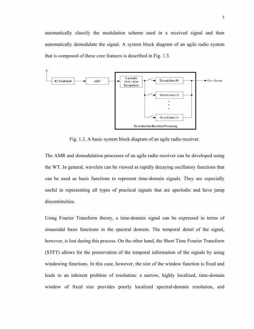
automatically classify the modulation scheme used in a received signal and then
automatically demodulate the signal. A system block diagram of an agile radio system
that is composed of these core features is described in Fig. 1.3.
Fig. 1.3. A basic system block diagram of an agile radio receiver.
The AMR and demodulation processes of an agile radio receiver can be developed using
the WT. In general, wavelets can be viewed as rapidly decaying oscillatory functions that
can be used as basis functions to represent time-domain signals. They are especially
useful in representing all types of practical signals that are aperiodic and have jump
discontinuities.
Using Fourier Transform theory, a time-domain signal can be expressed in terms of
sinusoidal basis functions in the spectral domain. The temporal detail of the signal,
however, is lost during this process. On the other hand, the Short Time Fourier Transform
(STFT) allows for the preservation of the temporal information of the signals by using
windowing functions. In this case, however, the size of the window function is fixed and
leads to an inherent problem of resolution: a narrow, highly localized, time-domain
window of fixed size provides poorly localized spectral-domain resolution, and
6
conversely a poorly-localized temporal window provides highly localized spectral
resolution. This drawback associated with fixed window sizes is especially problematic in
the analysis of digitally modulated communications signals. An advantageous situation
would be when the size of the window function can be altered to accommodate variations
in the phase and frequency of a signal.
The WT provides the feature of flexible window functions. In the WT, a window
function, i.e., a wavelet can be translated and dilated in time. The dilation of wavelets
allows for the variation of the size of wavelet windows to a specific temporal resolution.
The translated and dilated wavelets at different levels of resolution are cross-correlated
with the signal, resulting in the desired wavelet coefficients. These wavelet coefficients
implicitly contain the frequency information of the original signal, and explicitly preserve
the temporal information of the signal.
From the perspective of fundamental system development, the WT can be used to
develop a wavelet-based signal processing platform for agile radio systems. The agile
nature of a receiver is established using a WT-based AMR process and a subsequent
Automatic Demodulation process.
A system-level block diagram of such a Wavelet Platform is in Fig. 1.4. The Wavelet
Platform in the figure consists of five major components:
1. De-Noising: WT-based de-noising methods have been well established. De-
noising a corrupted received signal prior to processing it further would be a
valuable feature included in the Wavelet Platform.
2. Channel Estimation: Electrical characterization of the medium through which a

7
signal is propagating is performed in this operation. In addition, channel
estimation serves to restore signal features prior to WT-based AMR and
demodulation processes in order to improve performance.
3. Channel Equalization: The mitigation of unwanted channel effects present in
received signals is a desirable signal conditioning step before invoking the AMR
process.
4. AMR: This is a core feature of the Wavelet Platform. This processor
automatically identifies the modulation scheme of a received signal.
5. Demodulation: Automation demodulation is the second core feature of the
Wavelet Platform. After the modulation scheme of the unknown received signal is
recognized, the signal is then jointly and automatically demodulated appropriately
to recover the transmitted information.
Baseband Processor Modulator Front-End
Processing
Front-End Processing
Baseband Processor
Baseband Data
Recovered Baseband Data
Transmitter
Receiver
Channel Estimation
Channel Equalization
Automatic Modulation Recognition
Demodulator De-Noising
Wavelet Platform
Fig. 1.4. System-level block diagram of an agile radio transceiver based on the Wavelet
Platform [2].

8
In Fig. 1.4, both a transmitter and a receiver are shown as being part of an agile
transceiver. Major sub-systems of the receiver are implemented in the context of the
Wavelet Platform. In this transceiver, the transmitter operation is partially controlled by
the Wavelet Platform. The dashed lines serve to indicate feedback provided by the
Wavelet Platform to sub-systems in the transmitter. The information fed back can be
used to alter transmission characteristics such as the modulation scheme, carrier
frequency, etc., as needed. This functionality is yet another feature of agility possessed
by the wavelet-based transceiver.
In brief, the intention of developing wavelet-based AMR and automatic Demodulation
techniques is to advance the state of the art of communication systems by providing a
fundamental step towards interoperability between communications standards through the
use of wavelet transforms.
1.2 Objectives of the Dissertation
The primary objectives of this research work are:
1. To devise a technique for choosing a suitable wavelet(s) for use in both the AMR
and Demodulation processes.
2. Invention of a technique for choosing wavelet-domain signatures that are needed
for both the AMR and Demodulation processes.
3. Invention of techniques for AMR and automatic Demodulation using appropriate
wavelet-domain signatures, and evaluation of the performance of these new
techniques.
4. Compare the performance of the WT-based AMR and Demodulation

9
methodologies with results obtained using other methodologies that have been
reported in the literature.
The WT-based AMR and Demodulation processes both use the Continuous Wavelet
Transform (CWT).
Automatic Modulation Recognition
AMR is to be carried out with the use of WD signatures, or feature templates, which
contain characteristic features of a particular modulation scheme expressed in the
wavelet-domain. The received signal is transformed into the wavelet-domain using the
CWT. The cross-correlations between the transformed received signal and the WD
signatures are computed to obtained decision variables. The decision variables are used in
decision-making operations comprising the AMR algorithm.
The AMR algorithm is developed using a hypothesis testing methodology. The efficacy
of the AMR algorithm is validated using computer simulations. The simulations are
Monte Carlo experiments conducted in a manner so as to provide statistically significant
results.
Demodulation
WT-based Demodulation is developed based on the cross-correlations of WD signatures
with a received signal whose modulation technique has been classified. Demodulation
algorithms are specifically developed for each of the modulation schemes considered in
this work. The BER performances of the demodulation algorithms are compared with the
traditional matched filter-based BER performances for each modulation scheme. The
received signals have been corrupted by Additive White Gaussian Noise (AWGN) of

10
varying power levels.
Modulation Schemes
The modulation schemes considered in this research work are presented below. Some of
the current, planned, and future applications using the respective schemes are also
described.
1. M-ary Phase Shift Keying (M-PSK)
Table 1.1 MPSK modulation schemes and major applications
(a) BPSK IEEE 802.11a [1] and ZigBEE standards [3].
(b) QPSK IEEE 802.11b systems [4].
(c) 4π -QPSK Bluetooth 2 [5].
(d) 8-PSK Wireless communications systems applications.
11
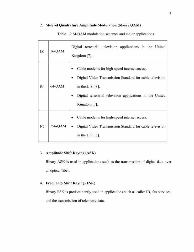
2. M-level Quadrature Amplitude Modulation (M-ary QAM)
Table 1.2 M-QAM modulation schemes and major applications
(a) 16-QAM Digital terrestrial television applications in the United
Kingdom [7].
(b) 64-QAM
• Cable modems for high-speed internet access.
• Digital Video Transmission Standard for cable television
in the U.S. [8].
• Digital terrestrial television applications in the United
Kingdom [7].
(c) 256-QAM
• Cable modems for high-speed internet access.
• Digital Video Transmission Standard for cable television
in the U.S. [8].
3. Amplitude Shift Keying (ASK)
Binary ASK is used in applications such as the transmission of digital data over
an optical fiber.
4. Frequency Shift Keying (FSK)
Binary FSK is predominantly used in applications such as caller ID, fax services,
and the transmission of telemetry data.

12
1.3 Major Contributions of the Dissertation
Among the many contributions of this research work, the following are considered to be
the most significant:
1. Development of a technique for choosing the suitable wavelet(s) for both the WD
AMR and the WD Demodulation processes.
2. Identification of WD signatures in digitally modulated communications signals
for use in WD AMR and WD Demodulation processes.
3. Development of new techniques for signal classification and demodulation of
digitally modulated communications signals using wavelet-domain signatures.
4. Introduction of a “moving origin” concept in order to recognize the different sizes
of square constellations for M-ary QAM signals based on a blind identification
process.
1.4 Organization of the Dissertation
This dissertation is composed of eight chapters. Chapter 1 introduces the framework of
agile transceivers and the problems being addressed in this study.
Chapter 2 contains an overview of existing AMR methodologies that use techniques
largely based on either a decision-theoretic approach, or a pattern recognition approach.
A summary of AMR techniques that employ WTs is also provided. In the remainder of
Chapter 2, an overview of demodulation techniques is provided, along with a survey of
demodulation techniques that are augmented by the use of de-noising procedures in the
wavelet-domain.
13
A brief primer on the CWT, along with descriptions of digital communications signals
and WD signature models, is provided in Chapter 3. The wavelet-domain cross-
correlation operation used in the AMR and demodulation algorithms is also introduced in
Chapter 3.
The preliminary setups required for both the AMR and the Demodulation processes are
described in Chapter 4. Several key parameters required for the AMR and Demodulation
processes are investigated in this chapter, including: 1.) Selection of WD signatures; 2.)
The length, or size, of the templates representing the WD signatures; and 3.) The suitable
choice of wavelet(s) used to transform the received signals.
This research work has produced two distinct WT-based AMR methodologies. Each is
based on a different type of template describing the communications signal features. The
two WT-based AMR methodologies involve:
1. Unique features templates
Templates that contain unique features of specific types of digitally modulated
signals that arise due to the symbol transitions inherent in the modulated
waveform structure.
2. Common features templates
Templates that contain variations of the sinusoidal feature within a symbol period
of different modulation schemes. The sinusoidal feature within a symbol is
common in all modulation schemes arising from either the carrier, or variations in
the carrier signal.
Two different AMR algorithms have been developed based on these two types of

14
templates.
AMR using unique features templates is considered in Chapter 5. In this chapter detailed
design procedures for the AMR algorithm, results of computer simulation experiments,
and comparisons of the results with the existing literature are provided.
In Chapter 6, AMR using common features templates is developed. The AMR algorithm
based on the common features templates, the simulation results, and comparisons of
results are described in detail.
In Chapter 7, the techniques used for automatic signal demodulation in the wavelet-
domain are presented. The BER performances of the WT-based demodulation of the
various modulation schemes are compared with the relevant matched filter-based BER
performances.
Finally, in Chapter 8, the important features of the AMR and Demodulation processes
invented in this dissertation are summarized; extensions of the work are identified for
possible future investigation; and, the conclusions of this research work are provided.
15
Chapter 2
Literature Survey
In this chapter, a survey of the literature on AMR methodologies and demodulation
techniques is presented. The survey is sub-divided into two main sections. The first
section is on AMR, and consists of:
1. Decision-theoretic approaches,
2. Pattern recognition techniques, and
3. Methods that have already been developed using the wavelet transform.
The second section is a survey of the demodulation techniques that have been reported in
the literature.
2.1 Automatic Modulation Recognition Techniques
Automatic Modulation Recognition techniques [9]-[64] have been explored in detail
since the 1980s. Several techniques have been developed to perform signal identification.
AMR techniques can be fundamentally classified into two main categories: techniques
utilizing a decision-theoretic approach [9]-[35], and techniques utilizing pattern
recognition approaches [36]-[47].
In order to augment, the AMR process, recently Support Vector Machines (SVMs) and
Artificial Neural Networks (ANNs) have been used with various decision-theoretic and
pattern recognition approaches to improve the overall modulation recognition process.
16
Both SVMs and ANNs also have been used in conjunction with wavelet transform-based
techniques for the purpose of modulation classification.
Most of the work reported in the literature is largely theoretical. In most cases, however,
the realization of the techniques in a hardware format for use in communications systems
is either absent, or minimally developed. Techniques for AMR are challenging since
there is no a priori information about the signals and other parameters at the receiver
such as the signal power, carrier frequency, carrier phase, Signal-to-Noise Ratio (SNR),
synchronization, etc.
The remainder of this section contains a survey of existing methods for AMR. In
particular, the decision-theoretic approach, the pattern recognition approach, wavelet-
based techniques, and recent trends in AMR research will be presented.
2.1.1 Techniques Based on the Decision-Theoretic Approach
In this popular approach, decision theory is applied to the problem of AMR. Specifically,
upon reception, several statistical parameters, e.g., variance, mean, average power, of a
signal are computed by the communications receivers. The same statistical parameters are
also computed beforehand for the ideal cases of several modulation types. The statistics
of the received signal are then correlated with those of the ideal cases, and decisions as to
which modulation scheme is active are then made. Some of the work reported in the
literature makes use of likelihood functions in conjunction with specific statistical
parameters to distinguish between modulation schemes.

17
In the literature, both analog and digital modulation schemes are reported to have been
identified successfully by the use of decision-theoretic approaches. Depending on the
AMR techniques used, different signal parameters and decision variables are extracted in
order to perform modulation type classification. The variety of approaches in the
literature includes:
• Statistical parameters with new 4th order cumulants [18]
• Constellation rotation of the received symbols and a 4th order cumulant of a
1-D distribution of the signal’s in-phase component [21]
• Combination of high-order mixed moments [22]
• The ratio of the power of the primary spectral line to the rest of the lines in
the Power Spectral Density (PSD), the number of notable spectral lines in the
PSD, the ratio of the Cyclic Spectral Density (CSD) function maximum
modulus at two different cyclic frequencies, the number of notable spectral
lines in the CSD [23]
• Envelope features based on the 2nd and 4th-order moments of the signal
envelope [24]
• The ratio of the variance to mean square of the normalized instantaneous
envelope of the signal [25]
• Bayesian likelihood function [25]
• Two-element antenna with maximum likelihood function [27]
• The maximum value of power spectral density of the normalized-centered
instantaneous amplitude, standard deviation of the absolute value of the
18
centered non-linear component of the instantaneous phase in the non-weak
intervals of a signal segment, the standard deviation of the direct (not
absolute) value of the centered non-linear component of the instantaneous
phase, the standard deviation of the absolute value of the normalized
instantaneous amplitude; and the standard deviation of the absolute value of
the normalized instantaneous frequency over different symbol periods are
used in [32].
2.1.2 Techniques Based on the Pattern Recognition Approach
In this section, several studies on AMR using pattern recognition approaches that have
been reported in the literature are presented. The most common and direct is the use of
histograms to count the number of occurrences of the instantaneous amplitude,
instantaneous frequency, and instantaneous phase of a received signal [45]-[46]. In these
studies, the communications signals considered were Amplitude Modulation (AM),
BASK, BFSK, 4-FSK, BPSK, QPSK, and 8-PSK. Another study reported in the literature
utilized the amplitude histogram, the signal bandwidth, and the relationship between
spectral components [46]. All of these parameters were obtained from the instantaneous
amplitude of the Intermediate Frequency (IF) signal spectrum.
A survey paper published in 2000 reported that using of statistical parameters together
with a pattern recognition approach can be applied to AMR [42]. The specific statistical
features considered in that study were:
• Kurtosis of the signal envelope
• Variance of the derivative of the Power Spectral Density (PSD) of the signal

19
• Mean of the absolute value of the signal frequency.
The digitally modulated communications signals considered in that study were ASK,
FSK, 4-Differential Phase Shift Keying (4-DPSK) and 16-QAM. Furthermore, a
classifier based on fuzzy logic was also utilized to distinguish between the various
signals. The rate of correct classification was reported to be 90% at SNR = 5 dB, but
rapidly reduced to 0% at SNR = 0 dB.
2.1.3 The Use of Artificial Neural Networks and Support Vector Machines for
Modulation Recognition
In recent years, newer methods for modulation classification based on a combination of
the decision-theoretic approach and other computational techniques such as SVMs [11]-
[13] and ANNs [14]-[16] have been developed. These new methods provide higher
accuracy of classification when communications signals are subject to noise and channel
impairments. The ANNs and SVM techniques have also been used in conjunction with
WTs [49], [56].
SVM is a mathematical technique which maps the input data, which are the statistical
parameters of the received signals in this case, to a higher-dimensional space. With the
use of an appropriate kernel function, the two sets of data points are separated by a
hyperplane. By separating the data representing the statistical parameters of the received
signal, modulation classification can be carried out. ANNs are a rather new technique
used in applications requiring computational decision-making. Multiple input stimuli are
provided to an ANN and are propagated through an interconnected network of nodes.
Each node has the ability to assign a weight to each input signal. However, ANNs also
20
have the ability to adaptively change these weights based on the specific decision-making
mathematical model chosen for the ANN. Using signal parameters obtained from either
the decision-theoretic, or pattern recognition-based methods, ANNs can be used for
modulation classification. In addition, the adaptive learning ability of ANNs is especially
useful for the classification of communications signals that are subject to noise and
channel impairments.
In [56], an ANN and the WT were used in order to increase the detection probability of a
code acquisition system. The WT was used to extract the structural parameters, i.e.,
signal power and phase of the received signal. The Morlet wavelet family was used in
this method. Specifically, the Back Propagation (BP) ANN was used for template
matching in conjunction with the structural parameters to achieve signal identification.
The rate of correct classification was reported to be approximately 94%, however, the
specific details about the noise scenarios applied to the test signals were omitted. Another
study employed neural networks and the DWT to obtain the Shannon entropy of the input
signals [55]. The calculated entropy was used to train the BP ANN. The signal was
processed using three different signal processing techniques, such as Fast Fourier
Transform (FFT), power spectral density estimator, and entropy in the WD. These
techniques were used in conjunction with the ANN in order to perform modulation
recognition. It was concluded, however, that the use of entropy for modulation
classification was an unsuitable method when compared to other methods.
In [49], an SVM-based modulation classification method was developed. In that method,
the Haar wavelet was used as the kernel function. BPSK, QPSK, and AM signals,
corrupted by additive band-limited Gaussian noise, were used as test signals in the

21
reported work. The rate of correct classification was 84% in the presence of band-limited
Gaussian noise.
2.1.4 Wavelet Transform-Based Techniques
WTs have been used for signal identification in a wide variety of areas, such as, medical
applications, manufacturing processing, fault detection in a power system, and image
processing. There are also a few publications that have used WT for AMR [48]-[64].
One popular WT-based approach involves computing the histogram of the wavelet
coefficients of the received signals and then counting the number of peaks in the
histogram in order to distinguish between PSK and FSK [54]; QPSK and GMSK [48],
[61]; and M-QAM and M-ASK [50].
In [54], the method used to distinguish PSK and FSK signals is to determine the number
of distinct histogram ordinate levels reached by the histogram data peaks. The distinct
levels are used as thresholds in a subsequent decision-making step. Hence, the number
M of distinct levels is used to identify the M-ary modulated signals. Fig. 2.1 shows the
histogram for BPSK, QPSK, BFSK and 4-FSK signals. The dotted horizontal lines in Fig.
2.1 indicate the thresholds for the various M-ary modulation schemes. The success rate
of modulation classification was reported to be 100% at an SNR of 13 dB, 99% at an
SNR of 10 dB, and 97% at an SNR of 8 dB.
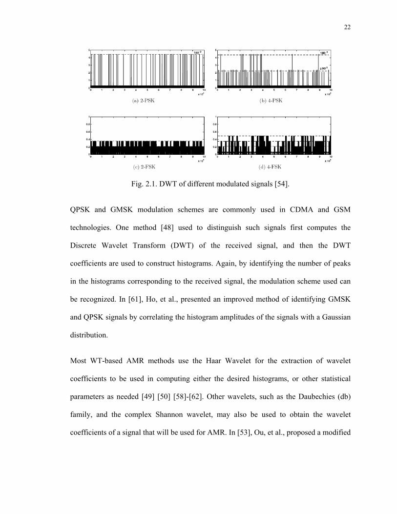
22
Fig. 2.1. DWT of different modulated signals [54].
QPSK and GMSK modulation schemes are commonly used in CDMA and GSM
technologies. One method [48] used to distinguish such signals first computes the
Discrete Wavelet Transform (DWT) of the received signal, and then the DWT
coefficients are used to construct histograms. Again, by identifying the number of peaks
in the histograms corresponding to the received signal, the modulation scheme used can
be recognized. In [61], Ho, et al., presented an improved method of identifying GMSK
and QPSK signals by correlating the histogram amplitudes of the signals with a Gaussian
distribution.
Most WT-based AMR methods use the Haar Wavelet for the extraction of wavelet
coefficients to be used in computing either the desired histograms, or other statistical
parameters as needed [49] [50] [58]-[62]. Other wavelets, such as the Daubechies (db)
family, and the complex Shannon wavelet, may also be used to obtain the wavelet
coefficients of a signal that will be used for AMR. In [53], Ou, et al., proposed a modified
23
Haar wavelet as the mother wavelet to extract the wavelet coefficients used to compute
the histogram.
Other methods in conjunction with the WT-based methods have also been introduced for
use in AMR. WT-based methods have also been combined with SVMs [49] and ANNs
[55]-[56]. In these cases, statistical parameters, such as the variance of the received
signal, and also the normalization of the signals, are computed for use as decision metrics
in the AMR process [58] [59] [62].
In [51], Chen, et al., proposed an algorithm which could identify signals in either the
inter-class, or intra-class by combining both WT and likelihood functions, which is
known as the decision-theoretic approach in the literature. The success rate of this
method is above 90% with a Carrier-to-Noise Ratio (CNR) of 13 dB and above.
Most of the literature involving the WT for AMR employs the Haar, Daubechies,
complex Shannon and Morlet wavelets. Most studies are based on the computation of the
histogram for the wavelet coefficients so as to identifying the number of peaks. However,
the drawback of this method is that only intra-class signals can be identified. Methods for
the identification of inter-class signals are still underdeveloped.
2.2 Techniques for Demodulation of Digital Data
Traditionally, demodulation techniques are based on the concept of matched filtering
[66]-[67] applied to the detection of digitally modulated communications signals.
Matched filtering methods are based on the cross-correlation of the basis functions with
the received communications signals in order to detect the presence, or absence, of the
24
basis function contained in the unknown signal. Using a subsequent Bayesian detector,
the baseband data bit sequence can be recovered.
Only one technique involving the use of WT in improving the demodulation of
communications signal has been developed. The approach used is to de-noise received
signals prior to demodulation using a standard matched filtering-based method [68]-[69].
In the work reported in [68], the signal was corrupted by AWGN resulting in SNR values
in the range of -3 dB to 3 dB, and the Haar wavelet was used in implementing the DWT.
It was determined that wavelet de-noising requires multiple samples per symbol to be
effective.
In [69], the use of different wavelets for signal decomposition employing the DWT was
presented. Both soft- and hard-thresholding were applied to the wavelet coefficients of
noisy communications signal prior to invoking the matched filter-based demodulation
method. PSK signal families were considered in this study. Signals were corrupted by
AWGN yielding SNR values in the range of -5 dB to 10 dB. The results show that the use
of wavelet-domain thresholding significantly improves the overall BER performance of
matched filter-based demodulation of PSK signals.
25
Chapter 3
Mathematical Preliminaries
Descriptions of the underlying theories of the CWT and the DWT are presented in
Section 3.1. Emphasis in the presentations, however, is on the CWT since that is the
transform used throughout this dissertation. In general terms, the CWT is defined as the
cross-correlation of a wavelet and a function of interest, while the DWT may be
described in terms of the filter theory approach of Multiresolution Analysis (MRA).
In Section 3.2, the time-domain mathematical models of the communications signals
investigated in this dissertation are presented. The WD AMR process developed in this
dissertation involves the cross-correlation of WD signatures and communications signals.
The cross-correlation operation in the WD is presented in Section 3.3.
3.1 An Overview of the Wavelet Transform
A brief introduction to the mathematical concept of the WT [65], [70]-[73] is presented in
this section. WTs can be essentially implemented using either the CWT or the DWT [76]-
[80]. The CWT is especially useful for the characterization (analysis) of signals, while
the DWT is used in signal and image processing for reconstruction and synthesis [79]. In
this dissertation, the CWT is used for both the AMR and the Demodulation processes.
Wavelets can be generally viewed as rapidly decaying oscillatory functions that may be
used as basis functions to represent signals. They are especially useful in representing all
types of signals that appear in practice with characteristics that are aperiodic and/or have
jump discontinuities. Some wavelets are compactly supported, i.e., localized in time, such

26
as the cubic B-spline wavelet [73]. Others, such as the Morlet wavelet, which is
constructed by modulating a sinusoidal function by a Gaussian function, are not [71].
Using Fourier transform theory, a time-domain signal can be expressed in terms of
sinusoidal functions (a continuous-time basis set) in the spectral domain. In this process,
however, the temporal detail of the signal is lost. By definition, Fourier transforms use
the entire time signal to produce the frequency-domain description of the signal. In the
case of transient signal analysis, the Short-Time Fourier Transform (STFT) [74] allows
for the preservation of the temporal information of the signal by using windowing
functions.
A carefully chosen user-defined window function is first multiplied with the signal
function, and then the Fourier transform of the resultant product function is taken. By
translating the window along the signal function in time, and then computing the Fourier
transform of each “windowed signal”, the STFT technique provides the ability to capture
the spectral content of the signal without losing the temporal content.
The fact that the window must be of fixed size, however, leads to an inherent problem of
resolution: a narrow, highly-localized, time-domain window of fixed size provides poorly
localized spectral-domain resolution, and conversely a broad, or non-localized, temporal
window provides highly localized spectral resolution. This drawback associated with
fixed window sizes is especially problematic in the analysis of digitally modulated
communications signals. An advantageous situation would be when the size of the
window function can be altered to accommodate variations of phase and frequency that
are characteristic of a digitally modulated communications signal.
27
In order to overcome this problem, WTs may be used instead. In the WT, a window
function, i.e., a wavelet can be translated and dilated in time. The dilation of wavelets
allows for the variation in the size of wavelet windows so as to achieve a specific
temporal resolution. The translated and dilated wavelets at different level of resolution
are cross-correlated with the signal, resulting in the desired wavelet coefficients. These
wavelet coefficients implicitly contain the frequency information of the original signal,
and explicitly preserve the temporal information of the signal.
3.1.1 Review of the Continuous Wavelet Transform
In contrast with the Fourier transform and the STFT, the window functions of wavelet
transforms have the properties that the function ( )tψ averages to zero over all time and
has finite energy [65], i.e., ( ) 0t dtψ∞
−∞
=∫ and ( ) 2t dtψ
∞
−∞
< ∞∫ , respectively.
It follows that window functions so described, allow for not only temporal translation but
also for time dilation. In other words, the width of the windows can be varied to achieve a
required resolution in either the temporal or spectral domains. Such window functions are
called wavelets. Transforming, that is comparing translated and scaled (dilated) wavelets
with the original signal yields correlation coefficients. In this way, at different scales,
correlation coefficients contain the frequency content of the original signal while
automatically preserving the temporal information of the signal.
The CWT, for a given wavelet ( )tψ , is formally defined as
28
( ) ( ) ( )*,, a bW a b f t t dtψ
∞
−∞
= ∫ (3.1)
where ( ),1
a bt bt
aaψ ψ −⎛ ⎞≡ ⎜ ⎟
⎝ ⎠ , ( )f t is the function to be transformed, a is the scale, or
dilation, variable and b is the translation variable.
MIN MAX
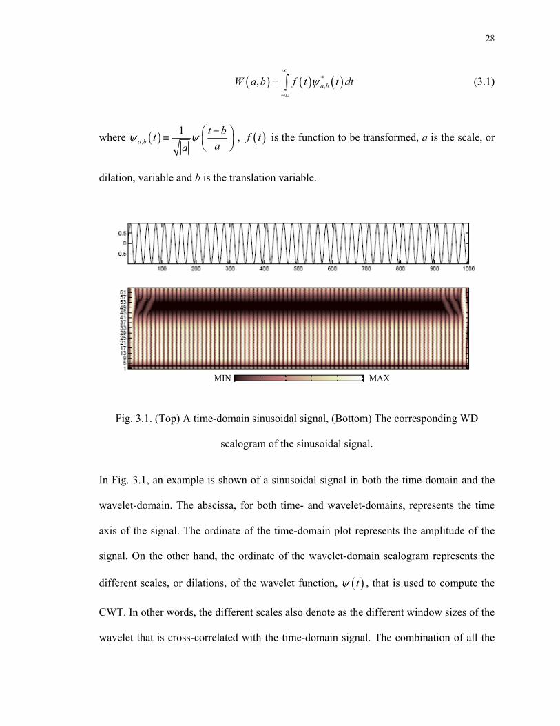
Fig. 3.1. (Top) A time-domain sinusoidal signal, (Bottom) The corresponding WD
scalogram of the sinusoidal signal.
In Fig. 3.1, an example is shown of a sinusoidal signal in both the time-domain and the
wavelet-domain. The abscissa, for both time- and wavelet-domains, represents the time
axis of the signal. The ordinate of the time-domain plot represents the amplitude of the
signal. On the other hand, the ordinate of the wavelet-domain scalogram represents the
different scales, or dilations, of the wavelet function, ( )tψ , that is used to compute the
CWT. In other words, the different scales also denote as the different window sizes of the
wavelet that is cross-correlated with the time-domain signal. The combination of all the
29
cross-correlation values (also known as the wavelet coefficients) for the different
dilations of the wavelet function, ( )tψ , makes up the scalogram. The different scales are
defined as the levels of resolution. The term levels of resolution is used in the remainder
of the dissertation.
On examining the fractal patterns of the segments appearing in the scalograms, it is seen
that structural details are present in two-dimensions (translation and scale) when one-
dimensional time-domain modulated signals are transformed into the WD. At some levels
of resolution in the WD, the signals are represented richly. While at other levels of
resolution the representation of the signal energy content is very weak. In the WD
scalogram shown in Fig. 3.1 (Bottom), the darker areas represent smaller cross-
correlation values obtained when the windowed time-domain signal is compared with a
wavelet of choice. The lighter areas in the scalogram represent larger magnitude wavelet
coefficients obtained with the windowed signal and the choice of wavelet. This particular
characteristic of the scalogram data is utilized advantageously in the WD AMR process.
Wavelets that are used for the CWT are typically required to satisfy the following
properties [83]:
i. Admissibility: Wavelets are required to be square integrable functions and
must not have a non-zero component at zero frequency. It is important that this
property be satisfied in order for the inverse CWT to be defined.
Mathematically, this condition is described as
30
( ) 2
c dψ
ωω
ω∞
−∞
Ψ= < +∞∫ (3.2)
where ( )ωΨ is the Fourier transform of the wavelet ( )tψ , and cψ is the
admissibility constant.
ii. Regularity: This condition ensures that the wavelet transform coefficients,
obtained using (3.1), decrease quickly in magnitude as the dilation changes. By
doing this, the wavelets can be very highly localized in time without causing an
unbounded time-bandwidth product.
Therefore, if a wavelet satisfies the condition that
( ) 0ppM t t dtψ
∞
−∞= =∫ for 0,1, 2, ,p n= (3.3)
where pM is the pth moment of the wavelet, then the wavelet is said to be of
order n.
iii. Linear Transformations: The wavelet transform, ( ),fW a b , must satisfy the
following conditions:
a) Superposition: ( ) ( ) ( )1 2 1 2
, , ,f f f fW a b W a b W a b+ = +
b) Translation: ( ) ( ) ( ) ( )0 0, ,f tf t tW a b W a b t− = −
c) Rescaling: ( ) ( ) ( ) ( )1 2 , ,f tm f mtW a b W ma mb= .
(3.4a)
(3.4b)
(3.4c)
By using the CWT, a broad class of communications signals can be expressed in terms of
wavelets belonging to different wavelet families. The results of such CWT operations are
wavelet coefficients that are specific to each combination of signal and wavelet. More
31
precisely, the wavelet coefficients may be obtained for different scales and translations of
the wavelet. By identifying the changes in the wavelet coefficients of a communications
signal, the characteristic amplitude, phase and frequency fluctuations inherent in a
communications signal can be identified.
3.1.2 Review of Multiresolution Analysis and the Discrete Wavelet Transform
The Digital Signal Processing (DSP) technique of MRA is based on the use of
orthonormal wavelet bases for signal analysis [70], [82]. In this technique, a sampled
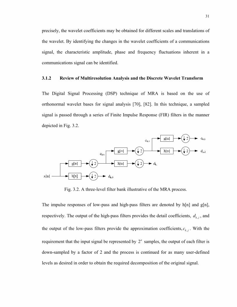
signal is passed through a series of Finite Impulse Response (FIR) filters in the manner
depicted in Fig. 3.2.
Fig. 3.2. A three-level filter bank illustrative of the MRA process.
The impulse responses of low-pass and high-pass filters are denoted by h[n] and g[n],
respectively. The output of the high-pass filters provides the detail coefficients, ,k jd , and
the output of the low-pass filters provide the approximation coefficients, ,k jc . With the
requirement that the input signal be represented by 2n samples, the output of each filter is
down-sampled by a factor of 2 and the process is continued for as many user-defined
levels as desired in order to obtain the required decomposition of the original signal.

32
In order to use MRA to implement the DWT technique a scaling function, ( )tφ , is
defined as [77]
( ) ( ) ( )0
2 2N
mt h N m t mφ φ
=
= − −∑ (3.5)
where 1N + is the order of the filter and m indexes into the set of filter coefficients
under consideration. The mother wavelet, ( )tψ , can then be described in terms of the
scaling function, and the filter coefficients according to
( ) ( ) ( ) ( ) ( ) ( )0 0
2 2 2 1 2N N
m
m mt g m t m h N m t mψ φ φ
= =
′ ′= − = − − − −∑ ∑ . (3.6)
In this MRA approach of implementing the DWT both the detail and approximation
coefficients of an input signal can be computed at different levels of resolution, as
illustrated in Fig. 3.2. Practically, the DWT can be used for the compression of data
prior to transmission through a noisy channel, for the de-noising of signals acquired by a
communications receiver, reconstruction of time-domain signals described in the
wavelet-domain, etc. [83]
As mentioned earlier, in developing the WD AMR process in this dissertation, it has
been found that the CWT is more suitable than the DWT. In the case of CWT, the signal
is represented by wavelet coefficients at different levels of resolution, which preserves
most of the signal contents. The CWT is also particularly useful for capturing the jump
discontinuities present in a signal, which often occurs in digitally modulated
communications signals. On the other hand, the DWT performs a decimation of the
wavelet-coefficients that is attractive for use in decomposition of a signal. This is
particularly useful in de-noising operations performed on a noisy signal, however, it

33
doesn’t help to preserve the signal contents that would be needed for signal
classification. Hence, subsequent attention is focused on the CWT.
3.2 Digital Communications Signal Models
Four different families of digital modulation schemes are considered in this dissertation.
Specifically, binary and quaternary ASK and FSK signals, M-ary PSK signals for M = 2,
4, and 8, and multiple-level QAM signals for M = 4, 16, 64, and 256 are investigated in
conjunction with developing classification strategies for WD AMR.
The time-domain ASK signals are defined as
( ) ( )2 cos 2 , 0
0, otherwise
bi c b
i b
EA f t t Ts t T
π⎧
≤ ≤⎪= ⎨⎪⎩
(3.7)
where 1,2,3,4,...i = . The variable iA represents the different levels of amplitude in ASK
signals such that { }iA ∈ . In the case of BASK, two amplitudes, 1A and 2A , denote data
symbols ‘0’ and ‘1’, respectively. In the case of 4-ASK signals, the four amplitudes, 1A ,
2A , 3A , and 4A , correspond to the data symbols ‘00’, ‘01’, ‘10’, and ’11.’ The parameter
bE denotes the energy per symbol, bT denotes the temporal duration of the symbol, and
the carrier frequency is denoted by cf .
The time-domain FSK signals used are defined as [84]
( ) ( )2 cos 2 , 0
0, otherwise
bi b
i b
E f t t Ts t T
π⎧
≤ ≤⎪= ⎨⎪⎩
(3.8)
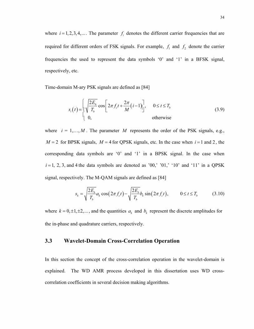
34
where 1,2,3,4,...i = . The parameter if denotes the different carrier frequencies that are
required for different orders of FSK signals. For example, 1f and 2f denote the carrier
frequencies the used to represent the data symbols ‘0’ and ‘1’ in a BFSK signal,
respectively, etc.
Time-domain M-ary PSK signals are defined as [84]
( ) ( )2 2cos 2 1 , 0
0, otherwise
bc b
i b
E f t i t Ts t T M
ππ⎧ ⎡ ⎤+ − ≤ ≤⎪ ⎢ ⎥= ⎣ ⎦⎨⎪⎩
(3.9)
where i = 1,…, M . The parameter M represents the order of the PSK signals, e.g.,
2M = for BPSK signals, 4M = for QPSK signals, etc. In the case when 1 and 2i = , the
corresponding data symbols are ‘0’ and ‘1’ in a BPSK signal. In the case when
1, 2, 3, and 4i = the data symbols are denoted as ’00,’ ’01,’ ‘10’ and ‘11’ in a QPSK
signal, respectively. The M-QAM signals are defined as [84]
( ) ( )2 2cos 2 sin 2 , 0b bk k c k c b
b b
E Es a f t b f t t TT T
π π= − ≤ ≤ (3.10)
where 0, 1, 2,...k = ± ± , and the quantities ka and kb represent the discrete amplitudes for
the in-phase and quadrature carriers, respectively.
3.3 Wavelet-Domain Cross-Correlation Operation
In this section the concept of the cross-correlation operation in the wavelet-domain is
explained. The WD AMR process developed in this dissertation uses WD cross-
correlation coefficients in several decision making algorithms.
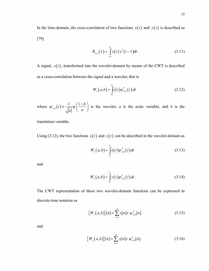
35
In the time-domain, the cross-correlation of two functions ( )x t and ( )y t is described as
[79]
( ) ( ) ( )*,x yR x t y t dtτ τ
∞
−∞
= −∫ . (3.11)
A signal, ( )s t , transformed into the wavelet-domain by means of the CWT is described
as a cross-correlation between the signal and a wavelet, that is
( ) ( ) ( )*,
0
,T
s a bW a b s t t dtψ= ∫ (3.12)
where ( ),1
a bt bt
aaψ ψ −⎛ ⎞≡ ⎜ ⎟
⎝ ⎠ is the wavelet, a is the scale variable, and b is the
translation variable.
Using (3.12), the two functions ( )x t and ( )y t can be described in the wavelet-domain as
( ) ( ) ( )*,
0
,T
x a bW a b x t t dtψ= ∫ (3.13)
and
( ) ( ) ( )*,
0
,T
y a bW a b y t t dtψ= ∫ . (3.14)
The CWT representation of these two wavelet-domain functions can be expressed in
discrete-time notation as
( ){ } *,
1, [ ] [ ] [ ]
N
x a bn
W a b n x n nψ=
=∑ i (3.15)
and
( ){ } *,
1, [ ] [ ] [ ]
N
y a bn
W a b n y n nψ=
=∑ i . (3.16)
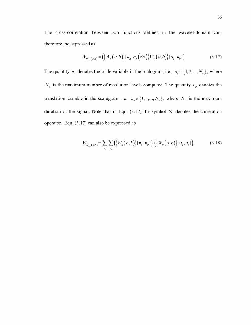
36
The cross-correlation between two functions defined in the wavelet-domain can,
therefore, be expressed as
( ) ( ){ }( ) ( ){ }( ), , , [ , ] , [ , ]
x y x a b y a bR a bW W a b n n W a b n n= ⊗ . (3.17)
The quantity an denotes the scale variable in the scalogram, i.e., { }1, 2,...,a an N∈ , where
aN is the maximum number of resolution levels computed. The quantity bn denotes the
translation variable in the scalogram, i.e., { }0,1,...,b bn N∈ , where bN is the maximum
duration of the signal. Note that in Eqn. (3.17) the symbol ⊗ denotes the correlation
operator. Eqn. (3.17) can also be expressed as
( ) ( ){ }( ) ( ){ }( ), , = , [ , ] , [ , ]
x ya b
x a b y a bR a bn n
W W a b n n W a b n n⋅∑∑ . (3.18)

37
Chapter 4
Setup for the Automatic Modulation Recognition Process
The Wavelet-Domain (WD) Automatic Modulation Recognition (AMR) process
developed in this dissertation is based on cross-correlating the Continuous Wavelet
Transform (CWT) of a digitally modulated signal of unknown modulation scheme, taken
to be at the input to a receiver, with a set of WD signatures that are locally stored
templates within a communications receiver. Therefore, in order to develop such a WD
AMR process, it is required to properly identify the WD signatures, or templates. At the
outset, a suitable wavelet must also be chosen in order to construct the templates for use
in the WD AMR process and also for performing the CWT of the received signal.
The methodologies to construct the templates are based on specific distinguishing
features of digitally modulated communications signals in both the time- and wavelet-
domains. Different temporal lengths of the WD signature templates are investigated in
order to enhance the cross-correlation operation used in conjunction with the decision
making algorithms. One immediate benefit of small WD signature lengths is a reduction
in the computational effort of the cross-correlation operations.
The choice of wavelet is arrived at based on the sensitivity of different candidate
wavelets to variations in the amplitude, frequency, and phase of a digitally modulated
signal. In this dissertation, the choice of a best-matched wavelet is selected based on the
largest cross-correlation result from among different WD signatures corresponding to a
total of 65 candidate wavelets. A matrix is formed using the cross-correlation values of
WD signatures for different signal features using various candidate wavelets. The values

38
are hard-thresholded in order to eliminate candidate wavelets which are not sensitive to a
particular distinguishing signal feature.
In this chapter, the main topics that are discussed include:
1. Techniques for template selection in the WD.
2. Variations in the temporal length, or size, of templates representing WD
signatures.
3. Choice of candidate wavelets based on cross-correlation values.
4.1 Template Selection for the Wavelet-Domain Automatic
Modulation Recognition Process
To develop the WD AMR process, it is necessary to properly identify the WD signatures,
or templates, that will be used in the AMR process. As seen from the definitions of the
digitally modulated signals given in Chapter 3, each of the digital modulation schemes
contain different types of features which can be extracted to serve as the WD signatures
for the WD AMR process. These features arise due to baseband symbol transitions, and
are seen to be variations in amplitude, frequency, and phase, of a carrier signal.
Figs. 4.1-4.3 illustrate BASK, BFSK, and BPSK signals with frame lengths that are 8
data-bearing symbols long in the time-domain, respectively. Symbol transitions, i.e., the
variations of amplitude, frequency, and phase, are enclosed in the boxes. In this
dissertation, such carrier transitions that arise between different symbols are used to
define the unique features templates.

39
0 100 200 300 400 500 600 700 800 900 1000-3
-2
-1
0
1
2
3
Time
Am
plitu
de
Fig. 4.1. Time-domain BASK signal with transitions contained within the box.
0 100 200 300 400 500 600 700 800 900 1000-2
-1
0
1
2
Time
Am
plitu
de
Fig. 4.2. Time-domain BFSK signal with transitions contained within the box.
0 100 200 300 400 500 600 700 800 900 1000-2
-1
0
1
2
Time
Am
plitu
de
Fig. 4.3. Time-domain BPSK signal with transitions contained within the box.
The wavelet-domain scalograms of the signals shown in Figs. 4.1-4.3 are provided in
Figs. 4.4-4.6, respectively with regions of the binary data transitions contained within the
box.

40
Values of Ca,b Coefficients for a = 1 2 3 4 5 ...
time (or space) b
scal
es a
100 200 300 400 500 600 700 800 900 1000 1 8 15 22 29 36 43 50 57 64 71 78 85 92 99106113120127
Fig. 4.4. Wavelet-domain scalogram of the BASK signal.
Values of Ca,b Coefficients for a = 1 2 3 4 5 ...
time (or space) b
scal
es a
100 200 300 400 500 600 700 800 900 1000 1 8 15 22 29 36 43 50 57 64 71 78 85 92 99106113120127
Fig. 4.5. Wavelet-domain scalogram of the BFSK signal.
Values of Ca,b Coefficients for a = 1 2 3 4 5 ...
time (or space) b
scal
es a
100 200 300 400 500 600 700 800 900 1000 1 8 15 22 29 36 43 50 57 64 71 78 85 92 99106113120127
Fig. 4.6. Wavelet-domain scalogram of the BPSK signal.
The WD representations of the unique features of BASK, BFSK, and BPSK signals,
which arise due to symbol transitions, are seen in Figs. 4.4-4.6. These features are stored
as templates representing the WD signatures of various modulation types for use in the
WD AMR process. While it is observed that the unique features are present in both the
time- and wavelet-domain templates, only WD signatures are used for the development
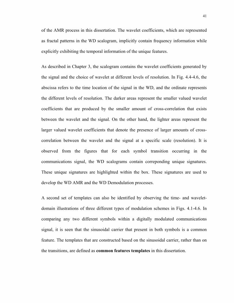
41
of the AMR process in this dissertation. The wavelet coefficients, which are represented
as fractal patterns in the WD scalogram, implicitly contain frequency information while
explicitly exhibiting the temporal information of the unique features.
As described in Chapter 3, the scalogram contains the wavelet coefficients generated by
the signal and the choice of wavelet at different levels of resolution. In Fig. 4.4-4.6, the
abscissa refers to the time location of the signal in the WD, and the ordinate represents
the different levels of resolution. The darker areas represent the smaller valued wavelet
coefficients that are produced by the smaller amount of cross-correlation that exists
between the wavelet and the signal. On the other hand, the lighter areas represent the
larger valued wavelet coefficients that denote the presence of larger amounts of cross-
correlation between the wavelet and the signal at a specific scale (resolution). It is
observed from the figures that for each symbol transition occurring in the
communications signal, the WD scalograms contain correponding unique signatures.
These unique signatures are highlighted within the box. These signatures are used to
develop the WD AMR and the WD Demodulation processes.
A second set of templates can also be identified by observing the time- and wavelet-
domain illustrations of three different types of modulation schemes in Figs. 4.1-4.6. In
comparing any two different symbols within a digitally modulated communications
signal, it is seen that the sinusoidal carrier that present in both symbols is a common
feature. The templates that are constructed based on the sinusoidal carrier, rather than on
the transitions, are defined as common features templates in this dissertation.
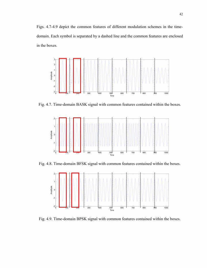
42
Figs. 4.7-4.9 depict the common features of different modulation schemes in the time-
domain. Each symbol is separated by a dashed line and the common features are enclosed
in the boxes.
0 100 200 300 400 500 600 700 800 900 1000-3
-2
-1
0
1
2
3
Time
Am
plitu
de
Fig. 4.7. Time-domain BASK signal with common features contained within the boxes.
0 100 200 300 400 500 600 700 800 900 1000-2
-1
0
1
2
Time
Am
plitu
de
Fig. 4.8. Time-domain BFSK signal with common features contained within the boxes.
0 100 200 300 400 500 600 700 800 900 1000-2
-1
0
1
2
Time
Am
plitu
de
Fig. 4.9. Time-domain BPSK signal with common features contained within the boxes.

43
From Figs. 4.7-4.9, it is observed that all three digitally modulated signals contain the
same common feature within different symbols, neglecting any variations in amplitude.
This common feature is the sinusoidal carrier. An exception to this rule is in the case of
BFSK, where another feature arises due to the variation frequency. Specifically, in BFSK
signals there may be two different carrier frequencies within a modulated signal
according to the definition of the modulation scheme and the actual data pattern. Since
the method used in extracting the common features templates is the same (i.e.,
windowing the sinusoidal carrier within a symbol to obtain a template), the BFSK
templates with different carrier frequencies are also grouped within the category of
common features templates.
The WD scalograms of the signals shown in Figs. 4.7-4.9, i.e., the plots that have
common features highlighted, are shown in Figs. 4.10-4.12, respectively. As seen in
these figures, the scalograms depict details of the time-domain signal structure at
different levels of resolution in the WD. In Figs. 4.10-4.12, the WD common features
templates for the three modulation schemes are the contents of the boxes. Unlike the
unique features templates representing symbol transitions, the common features templates
capture the modulation characteristics within a symbol period as shown in boxes within
these figures. The vertical dotted lines represent the symbol period boundaries within a
finite duration of an overall communications signal.
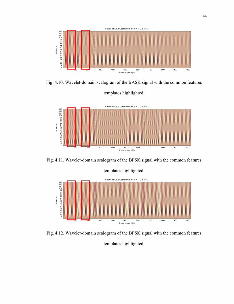
44
Values of Ca,b Coefficients for a = 1 2 3 4 5 ...
time (or space) b
scal
es a
100 200 300 400 500 600 700 800 900 1000 1 8 15 22 29 36 43 50 57 64 71 78 85 92 99106113120127
Fig. 4.10. Wavelet-domain scalogram of the BASK signal with the common features
templates highlighted.
Values of Ca,b Coefficients for a = 1 2 3 4 5 ...
time (or space) b
scal
es a
100 200 300 400 500 600 700 800 900 1000 1 8 15 22 29 36 43 50 57 64 71 78 85 92 99106113120127
Fig. 4.11. Wavelet-domain scalogram of the BFSK signal with the common features
templates highlighted.
Values of Ca,b Coefficients for a = 1 2 3 4 5 ...
time (or space) b
scal
es a
100 200 300 400 500 600 700 800 900 1000 1 8 15 22 29 36 43 50 57 64 71 78 85 92 99106113120127
Fig. 4.12. Wavelet-domain scalogram of the BPSK signal with the common features
templates highlighted.

45
From the various characteristics seen in Figs. 4.1-4.12, two distinct categories of
templates can be constructed, and therefore, two distinct WD AMR algorithms will be
developed. The two WD AMR algorithms are:
1. WD AMR process employing the unique features templates.
2. WD AMR process using the common features templates.
The observations that have been made thus far are based only on binary digitally
modulated communications signals. The same concepts, however, can be used in order to
construct the two categories of templates for signals associated with higher-order
modulation schemes. For example, unique features templates can also be extracted based
on the symbol transitions present in QPSK signals. Fig. 4.13 illustrates all of the possible
unique features in the WD for a QPSK signal. By the definition of a QPSK signal
described in (3.9), the signal is constructed based on different phase variations of
symbols corresponding to different data bits. Therefore, the unique features templates are
constructed based on symbol transitions, which arise from the QPSK signal phase
variations. There are a total of 16 unique features templates extracted for use in both the
WD AMR and Demodulation processes.
In Fig. 4.13, it is observed that each unique feature, arising due to symbol transitions, is
different from all of the other features. Therefore, it is anticipated that using these unique
features templates within the WD AMR process would result in a high rate of correct
classification for QPSK modulated signals. Furthermore, due to their uniqueness, these
templates can also be used advantageously to develop a robust WD Demodulation
algorithm.
46
Fig. 4.13. (a-q) WD scalograms of the unique features corresponding to all sixteen
symbol transitions in a QPSK signal.
As can be seen in the case of QPSK, the number of WD signatures required for the WD
AMR process increases for more complex modulation schemes. However, on the other
hand, the common features within the symbols of a QPSK signal are the same as those
for a BPSK signal, as illustrated in Fig. 4.14. Therefore, the same set of common features
templates, along with an appropiate hypothesis test, can be used to achieve classification
of a signal with unknown modulation type with reduced complexity. In the case of 4-
FSK there are four distinct common features due to the four different carrier frequencies
that are used to represent the baseband symbols. This can be seen in Fig. 4.15.

47
0 100 200 300 400 500 600 700 800 900 1000-2
-1
0
1
2
Time
Am
plitu
de
(a)
Values of Ca,b Coefficients for a = 1 2 3 4 5 ...
time (or space) b
scal
es a
100 200 300 400 500 600 700 800 900 1000 1 8 15 22 29 36 43 50 57 64 71 78 85 92 99106113120127
(b)
0 100 200 300 400 500 600 700 800 900 1000-2
-1
0
1
2
Time
Am
plitu
de
(c)
Values of Ca,b Coefficients for a = 1 2 3 4 5 ...
time (or space) b
scal
es a
100 200 300 400 500 600 700 800 900 1000 1 8 15 22 29 36 43 50 57 64 71 78 85 92 99106113120127
(d)
Fig. 4.14. (a) Time-domain BPSK signal, (b) WD scalogram for the BPSK signal, (c)
Time-domain QPSK signal, and (d) WD scalogram of the QPSK signal.

48
0 100 200 300 400 500 600 700 800 900 1000-2
-1
0
1
2
Time
Am
plitu
de
(a)
Values of Ca,b Coefficients for a = 1 2 3 4 5 ...
time (or space) b
scal
es a
100 200 300 400 500 600 700 800 900 1000 1 8 15 22 29 36 43 50 57 64 71 78 85 92 99106113120127
(b)
Fig. 4.15. (a) Time domain 4-FSK signal, and (b) WD scalogram of the 4-FSK signal.
Note again that higher-order ASK and PSK signals contain the same common features,
and therefore, the same set of common features templates are used in the WD AMR
process for these modulation schemes.
To summarize, two categories of templates have been identified to represent WD
signatures for use in the development of WD AMR. The templates in the first
category are called unique features templates, which contain carrier transition
features specific to different modulation schemes. The templates belonging to the
second category are called common features templates due to the fact that these
templates represent the common features of a sinusoidal carrier that are present in
different baseband symbols.
49
Chapter 5 will be focused on the development of a WD AMR algorithm using the unique
features templates, while Chapter 6 will describe a WD AMR algorithm using the
common features templates.
4.2 Mathematical Models of the Templates for Wavelet-Domain
Signatures
WD signatures of specific time-domain features of digitally modulated signals are used
for the AMR process in this dissertation. Details of the templates describing the WD
signatures were described in Section 4.1. There are two categories of templates for the
WD signatures, namely, the unique features templates and the common features
templates. Time-domain analytical representations of the templates are presented as
follows.
1. Unique Features Templates
These templates are described based on symbol transitions that occur within a
digitally modulated communications signal. Two unique features templates can
be extracted from each of the 3 binary digitally modulated signals. The piece-
wise continuous models of these templates are defined according to the
following:
i. For BASK signals, the two templates are defined as
( ) ( )( )
1 1 2,1
2 3 4
cos 2 , cos 2 ,
cBASK
c
A f t t t tp t
A f t t t tππ
< ≤⎧⎪= ⎨ < ≤⎪⎩ (4.1a)
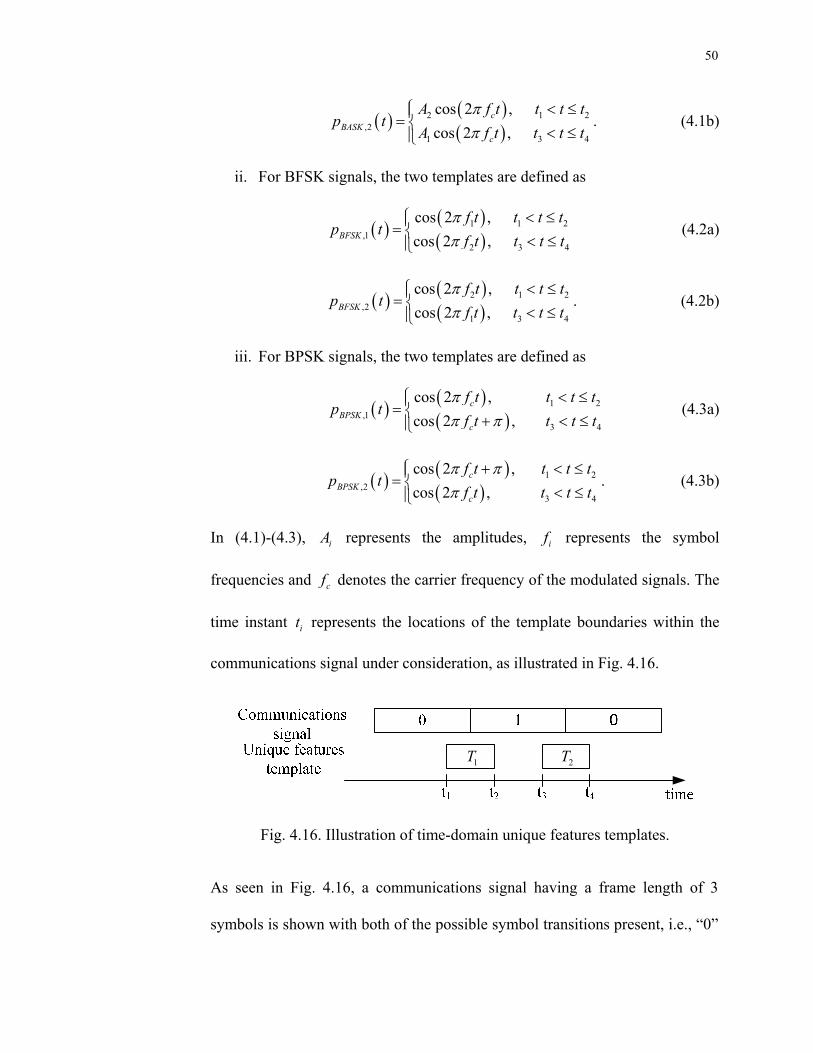
50
( ) ( )( )
2 1 2,2
1 3 4
cos 2 , cos 2 ,
cBASK
c
A f t t t tp t
A f t t t tππ
< ≤⎧⎪= ⎨ < ≤⎪⎩. (4.1b)
ii. For BFSK signals, the two templates are defined as
( ) ( )( )
1 1 2,1
2 3 4
cos 2 , cos 2 , BFSK
f t t t tp t
f t t t tππ
< ≤⎧⎪= ⎨ < ≤⎪⎩ (4.2a)
( ) ( )( )
2 1 2,2
1 3 4
cos 2 , cos 2 , BFSK
f t t t tp t
f t t t tππ
< ≤⎧⎪= ⎨ < ≤⎪⎩. (4.2b)
iii. For BPSK signals, the two templates are defined as
( ) ( )( )
1 2,1
3 4
cos 2 , cos 2 ,
cBPSK
c
f t t t tp t
f t t t tππ π
< ≤⎧⎪= ⎨ + < ≤⎪⎩ (4.3a)
( ) ( )( )
1 2,2
3 4
cos 2 , cos 2 ,
cBPSK
c
f t t t tp t
f t t t tπ ππ
+ < ≤⎧⎪= ⎨ < ≤⎪⎩. (4.3b)
In (4.1)-(4.3), iA represents the amplitudes, if represents the symbol
frequencies and cf denotes the carrier frequency of the modulated signals. The
time instant it represents the locations of the template boundaries within the
communications signal under consideration, as illustrated in Fig. 4.16.
1T 2T
Fig. 4.16. Illustration of time-domain unique features templates.
As seen in Fig. 4.16, a communications signal having a frame length of 3
symbols is shown with both of the possible symbol transitions present, i.e., “0”
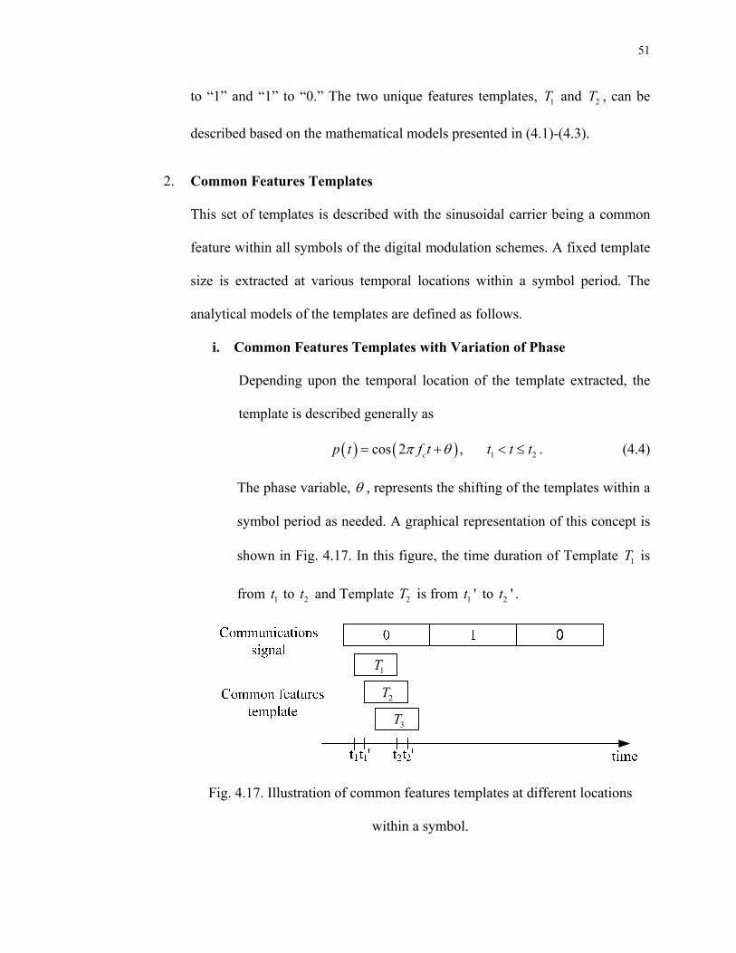
51
to “1” and “1” to “0.” The two unique features templates, 1T and 2T , can be
described based on the mathematical models presented in (4.1)-(4.3).
2. Common Features Templates
This set of templates is described with the sinusoidal carrier being a common
feature within all symbols of the digital modulation schemes. A fixed template
size is extracted at various temporal locations within a symbol period. The
analytical models of the templates are defined as follows.
i. Common Features Templates with Variation of Phase
Depending upon the temporal location of the template extracted, the
template is described generally as
( ) ( ) 1 2cos 2 , cp t f t t t tπ θ= + < ≤ . (4.4)
The phase variable, θ , represents the shifting of the templates within a
symbol period as needed. A graphical representation of this concept is
shown in Fig. 4.17. In this figure, the time duration of Template 1T is
from 1t to 2t and Template 2T is from 1 't to 2 't .
1T
2T
3T
Fig. 4.17. Illustration of common features templates at different locations
within a symbol.
52
ii. Common Features Templates with Different Frequencies
In an M-ary FSK signal, different carrier frequencies are used to
represent different data symbols within the modulated signal.
Therefore, another common features template can be defined
according to
( ) ( ) 1 2cos 2 , ip t f t t t tπ= < ≤ (4.5)
where if is the active carrier frequency in the specified symbol time
slot.
4.3 Determining the Length of the Templates for Wavelet-Domain
Signatures
In the AMR process that is developed in this dissertation, a wavelet-transformed received
signal of finite time duration is cross-correlated with WD signatures, which are also of
finite time duration. The WD signatures may be either unique features templates or
common features templates. In the WD cross-correlation operation, templates of finite
length, are slid across the communications signal, and then compared to it via correlation
in order to determine if the wavelet-transformed signal contains any features that are
similar to the WD signatures represented by the templates.
When unique features templates are used, these WD templates must be perfectly aligned
with the carrier transitions corresponding to each baseband symbol in the cross-
correlation operations. In order to ensure such alignment the duration, or length, of each
template must be a perfect divisor of the duration of each signal segment corresponding
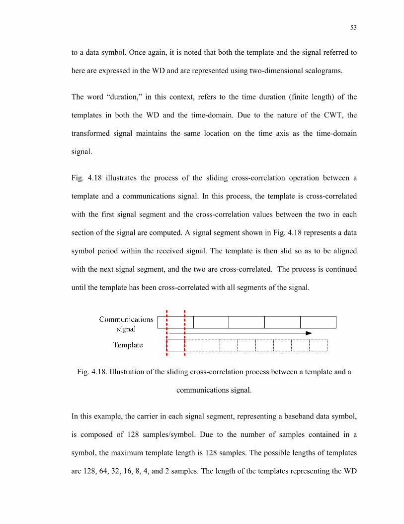
53
to a data symbol. Once again, it is noted that both the template and the signal referred to
here are expressed in the WD and are represented using two-dimensional scalograms.
The word “duration,” in this context, refers to the time duration (finite length) of the
templates in both the WD and the time-domain. Due to the nature of the CWT, the
transformed signal maintains the same location on the time axis as the time-domain
signal.
Fig. 4.18 illustrates the process of the sliding cross-correlation operation between a
template and a communications signal. In this process, the template is cross-correlated
with the first signal segment and the cross-correlation values between the two in each
section of the signal are computed. A signal segment shown in Fig. 4.18 represents a data
symbol period within the received signal. The template is then slid so as to be aligned
with the next signal segment, and the two are cross-correlated. The process is continued
until the template has been cross-correlated with all segments of the signal.
Fig. 4.18. Illustration of the sliding cross-correlation process between a template and a
communications signal.
In this example, the carrier in each signal segment, representing a baseband data symbol,
is composed of 128 samples/symbol. Due to the number of samples contained in a
symbol, the maximum template length is 128 samples. The possible lengths of templates
are 128, 64, 32, 16, 8, 4, and 2 samples. The length of the templates representing the WD

54
signatures, however, cannot be too short due to the loss of resolution in the WD
scalogram. The loss of resolution directly affects the performance of the WD AMR
process. A graphical representation of the sliding process with different template lengths
is shown in Fig. 4.19. For the sake of illustration, only templates of size 128, 64, and 32
samples are used.
Fig. 4.19. Graphical representation of the cross-correlation operation using different
template lengths.
The scalogram of a BPSK test signal with a frame length of 40 symbols, is shown in Fig.
4.20. The test signal is used to demonstrate the cross-correlation operation with different
lengths for the unique features templates, as described in Fig. 4.21. As seen in Figs. 4.22-
24, the cross-correlation results of the unique features templates with lengths of 32, 64,
and 128 samples when compared with the BPSK test signal are shown. It is observed
that that the longer the length of the template, the fewer the number of cross-correlation
peaks that are computed and available for decision making.

55
Values of Ca,b Coefficients for a = 1 2 3 4 5 ...
time (or space) b
scal
es a
500 1000 1500 2000 2500 1 8 15 22 29 36 43 50 57 64 71 78 85 92 99106113120127
Fig. 4.20. Scalogram of a BPSK test signal.
The choice of template length for both the WD AMR and Demodulation processes is 64
samples. The particular choice of 64 samples in a template maintains the required
resolution in the WD scalogram. Furthermore, using 64 samples does not increase the
computational effort in performing the cross-correlation operation as compared to when
templates consist of 128 samples. Another possible effect due to the different template
lengths is that of the WD AMR system robustness in the presence of AWGN. More
samples in a template (longer in length) may result in a higher possibility of error since
the WD AMR and the WD Demodulation processes are based on a cross-correlation
operations with the received, noisy signal and noise-free templates. A detail explanation
concerning the effect of noise is presented in Chapter 7.
Values of Ca,b Coefficients for a = 1 2 3 4 5 ...
time (or space) b
scal
es a
20 40 60 80 100 120 1 8 15 22 29 36 43 50 57 64 71 78 85 92 99106113120127
(a)
Values of Ca,b Coefficients for a = 1 2 3 4 5 ...
time (or space) b
scal
es a
10 20 30 40 50 60 1 8 15 22 29 36 43 50 57 64 71 78 85 92 99106113120127
(b)
Values of Ca,b Coefficients for a = 1 2 3 4 5 ...
time (or space) b
scal
es a
5 10 15 20 25 30 1 8 15 22 29 36 43 50 57 64 71 78 85 92 99106113120127
(c)
Fig. 4.21. WD unique features Template 1 with length of (a) 128 samples, (b) 64 samples,
and (c) 32 samples.

56
0 10 20 30 40 50 60 70 80-1.5
-1
-0.5
0
0.5
1
1.5
Am
plitd
ue
Fig. 4.22. Cross-correlation results using a unique features template that is 32 samples in
length.
0 5 10 15 20 25 30 35 40-3
-2
-1
0
1
2
3
Am
plitd
ue
Fig. 4.23. Cross-correlation results using a unique features template that is 64 samples in
length.
0 2 4 6 8 10 12 14 16 18 20-6
-4
-2
0
2
4
6
Am
plitd
ue
Fig. 4.24. Cross-correlation results using a unique features template that is 128 samples in
length.

57
4.4 Selection of Wavelets to be Used for Automatic Modulation
Recognition
Sixty-five wavelets are considered in this dissertation for possible use in constructing an
AMR processor. In order to find the most suitable wavelet, or wavelets, for use in the
WD AMR process, custom matrix images are generated. The images are based on the
auto- and cross-correlation data of the unique features templates and the common features
templates that had been constructed using the 65 different candidate wavelets.
The candidate wavelets considered in this study include:
1. Haar wavelet
2. Mexican wavelet
3. Morlet wavelet
4. Meyer wavelet
5. Discrete Meyer wavelet
6. The family of Daubechies wavelets (db1-db10)
7. Symlets ( sym2-sym8)
8. Coiflets (coif1-coif5)
9. Biorthogonal spline wavelets (bior1.1, 1.3, 1.5, 2.2, 2.4, 2.6, 2.8, 3.1, 3.3, 3.5, 3.7,
3.9, 4.4, 5.5, 6.8)
10. Reverse biorthogonal spline wavelets (rbio1.1, 1.3, 1.5, 2.2, 2.4, 2.6, 2.8, 3.1, 3.3,
3.5, 3.7, 3.9, 4.4, 5.5, 6.8)
11. The Gaussian wavelet family (gaus1-gaus8)

58
Since there are two categories of templates representing the WD signatures, i.e., unique
features templates and common features templates, two sets of matrix images are
developed to aid in the determination of the suitable choice of wavelet(s) for the WD
AMR process.
To summarize, the goals of this section are:
1. From the auto-correlations of all templates, to identify the wavelet(s) that
produces large magnitude results for all three modulation schemes (i.e. BASK,
BFSK, and BPSK).
2. To verify that the cross-correlations of all templates, i.e., the WD signatures
between the three modulation schemes are weak. This verification would
support the creation of an AMR process based on WD signatures.
4.4.1 Selection of Wavelets Using Unique Features Templates
Each of the binary digital modulation schemes, i.e., BASK, BFSK, and BPSK, produce
two unique features templates. For the purpose of clarity, the unique features template for
the transition from symbol ‘0’ to symbol ‘1’ is denoted as “Template 1,” and “Template
2” is used to denote transitions from symbol ‘1’ to symbol ‘0’. This nomenclature is used
for the unique features templates for all three binary modulation schemes.
The matrix image created in this section contains the cross-correlation values between all
unique features templates for all three modulation schemes. The matrix image is used to
help identify the most suitable wavelet(s) for WD AMR. Note that either Template 1, or
Template 2 for each of the modulation schemes could be used in this procedure. Of
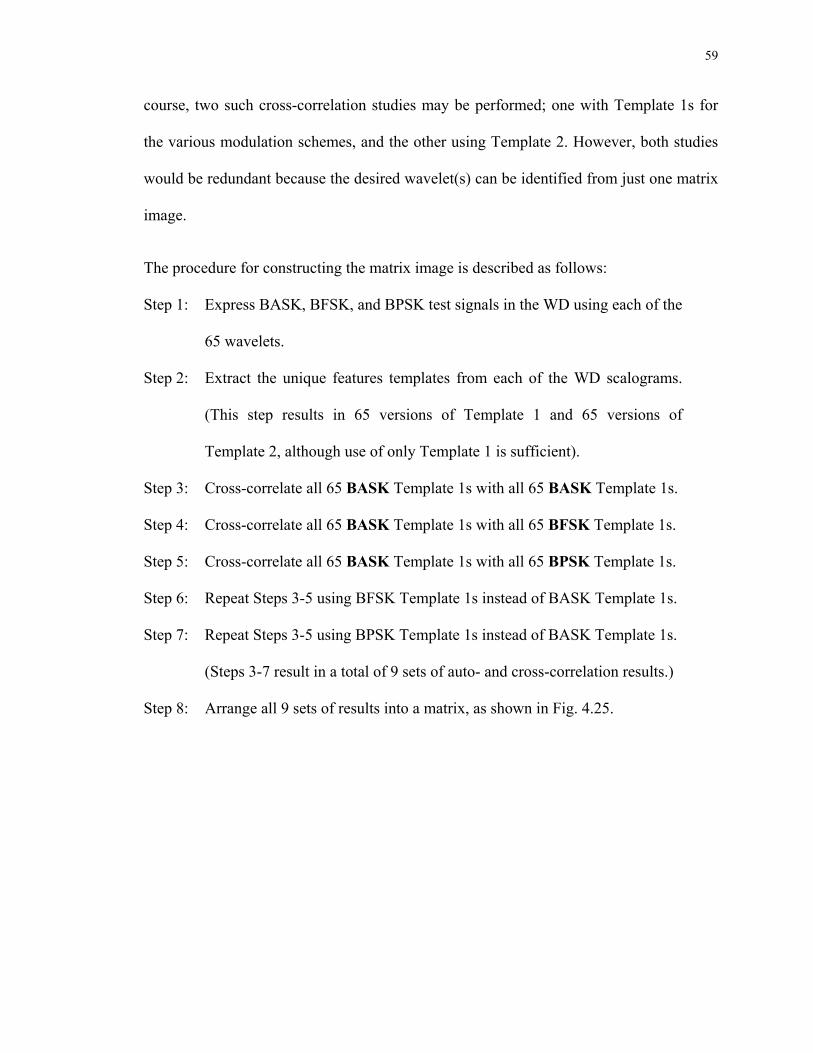
59
course, two such cross-correlation studies may be performed; one with Template 1s for
the various modulation schemes, and the other using Template 2. However, both studies
would be redundant because the desired wavelet(s) can be identified from just one matrix
image.
The procedure for constructing the matrix image is described as follows:
Step 1: Express BASK, BFSK, and BPSK test signals in the WD using each of the
65 wavelets.
Step 2: Extract the unique features templates from each of the WD scalograms.
(This step results in 65 versions of Template 1 and 65 versions of
Template 2, although use of only Template 1 is sufficient).
Step 3: Cross-correlate all 65 BASK Template 1s with all 65 BASK Template 1s.
Step 4: Cross-correlate all 65 BASK Template 1s with all 65 BFSK Template 1s.
Step 5: Cross-correlate all 65 BASK Template 1s with all 65 BPSK Template 1s.
Step 6: Repeat Steps 3-5 using BFSK Template 1s instead of BASK Template 1s.
Step 7: Repeat Steps 3-5 using BPSK Template 1s instead of BASK Template 1s.
(Steps 3-7 result in a total of 9 sets of auto- and cross-correlation results.)
Step 8: Arrange all 9 sets of results into a matrix, as shown in Fig. 4.25.
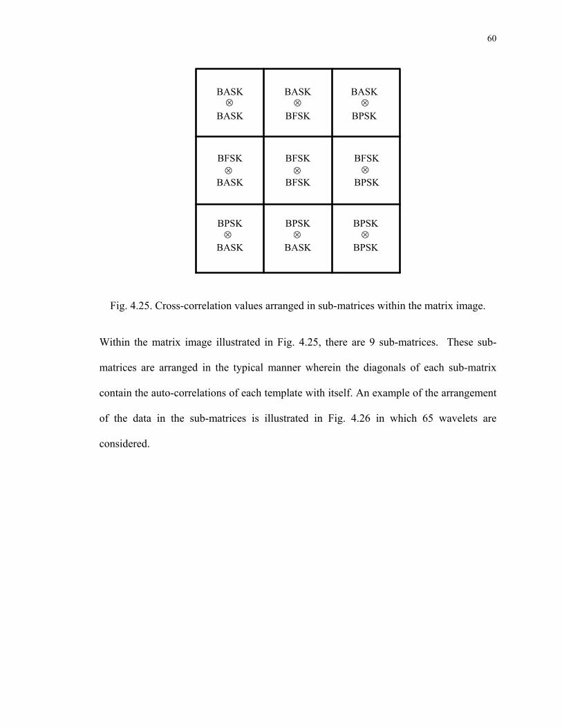
60
BASK
BASK
BASK
BFSK
BASK
BPSK
BFSK
BASK
BFSK
BFSK
BFSK
BPSK
BPSK
BASK
BPSK
BASK
BPSK
BPSK
⊗ ⊗ ⊗
⊗⊗⊗
⊗ ⊗⊗
Fig. 4.25. Cross-correlation values arranged in sub-matrices within the matrix image.
Within the matrix image illustrated in Fig. 4.25, there are 9 sub-matrices. These sub-
matrices are arranged in the typical manner wherein the diagonals of each sub-matrix
contain the auto-correlations of each template with itself. An example of the arrangement
of the data in the sub-matrices is illustrated in Fig. 4.26 in which 65 wavelets are
considered.

61
65 w
avel
ets
Fig. 4.26. An example of the construction of the sub-matrices.
As seen in Fig. 4.26, each cell in the sub-matrix contains the cross-correlation data of the
templates with specific candidate wavelets according to the header of each row and
column.
In this study only Template 1 has been used for all 3 modulation schemes. The auto- and
cross-correlations of all 65 Template 1s for all 3 modulation schemes are arranged in the
matrix image shown in Fig. 4.27.
In order to determine the most suitable wavelet(s) from examination of the matrix image,
the data are subjected to hard-thresholding. The first threshold value used is Δ= 0. Since
negative cross-correlation coefficients in this case imply that the two templates are
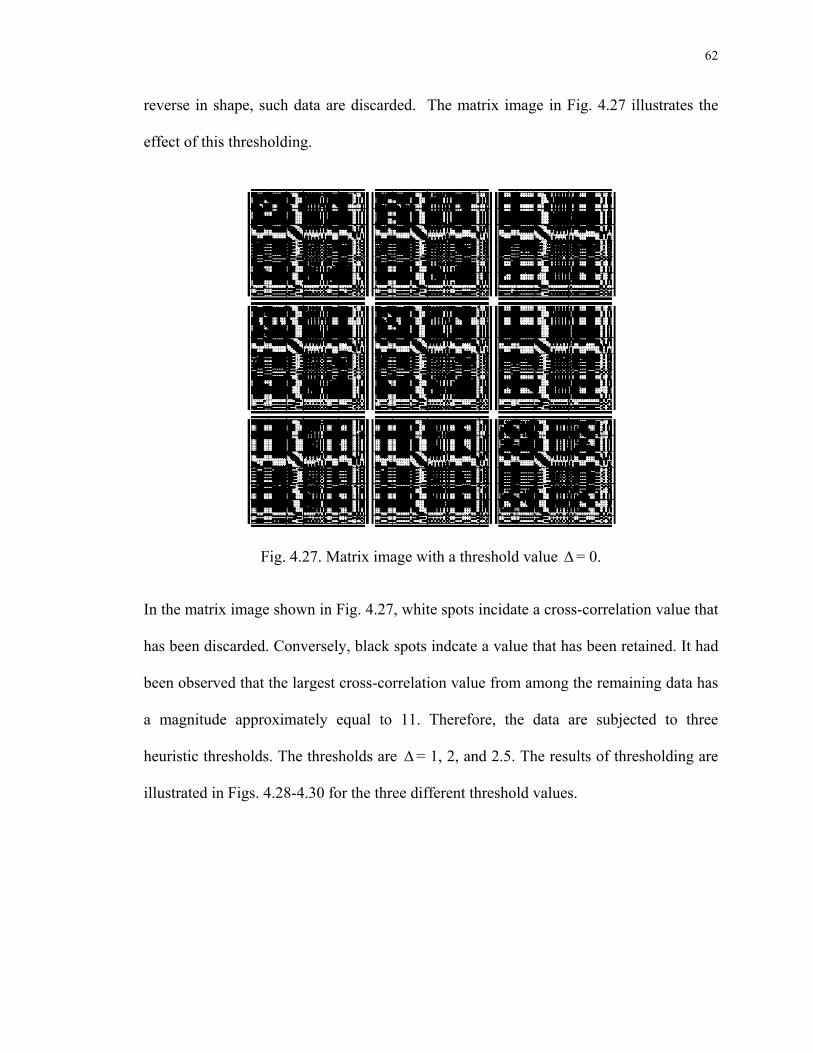
62
reverse in shape, such data are discarded. The matrix image in Fig. 4.27 illustrates the
effect of this thresholding.
Fig. 4.27. Matrix image with a threshold value Δ= 0.
In the matrix image shown in Fig. 4.27, white spots incidate a cross-correlation value that
has been discarded. Conversely, black spots indcate a value that has been retained. It had
been observed that the largest cross-correlation value from among the remaining data has
a magnitude approximately equal to 11. Therefore, the data are subjected to three
heuristic thresholds. The thresholds are Δ= 1, 2, and 2.5. The results of thresholding are
illustrated in Figs. 4.28-4.30 for the three different threshold values.

63
Fig. 4.28. Matrix image with a threshold value of Δ = 1.
In Fig. 4.28, the threshold value Δ = 1, is seen to be too low. This observation is made
because there are still too many large-valued cross-correlation data remaining. Due to
this, it is not possible to identify the desired wavelets, i.e., wavelets that produce
Template 1s that result in large magnitude correlation values for all of the three
modulation schemes.
A higher threshold value must, therefore, be applied. Next, the threshold value Δ = 2 is
used, and the resulting matrix image is shown in Fig. 4.29. In this image a suitable
wavelet is identifiable. The chosen wavelet is the Reverse Biorthogonal Spline 1.3 (rbio
1.3). The auto- and cross-correlation values corresponding to the templates based on this
wavelet are shown within the circles that are included in Fig. 4.29.

64
The solid circles indicate the auto-correlation values corresponding to the Template 1s
based on the rbio1.3 wavelet. The dotted circles indicate the locations of the cross-
correlation values of the templates that are based on rbio1.3. This observation is critical
for the AMR process since it implies that Template 1, based on rbio1.3, of one
modulation scheme will not strongly correlate with a unique feature of another
modulation scheme.
Fig. 4.29. Matrix image with a threshold value of Δ = 2.
For the sake of completeness, an even higher threshold value Δ = 2.5 is also used. The
resulting matrix image is provided in Fig. 4.30. It is seen that most results have been
discarded, and hence, no common wavelet(s) can be identified with this large of a
threshold.

65
Fig. 4.30. Matrix image with a threshold value of Δ = 2.5.
4.4.2 Selection of Wavelets Using Common Features Templates
The exact procedure used in Section 4.4.1 is now applied to determine the most suitable
wavelet(s) on which the common features templates can be based. The only difference in
this case is that the common features templates are used instead of the unique features
templates.
The common features templates to be used for the creation of the matrix image in this
case are highlighted in boxes in as shown Fig. 4.31. Once again the dotted vertical lines
in Fig. 4.31 indicate the symbol boundaries in the modulated signals.
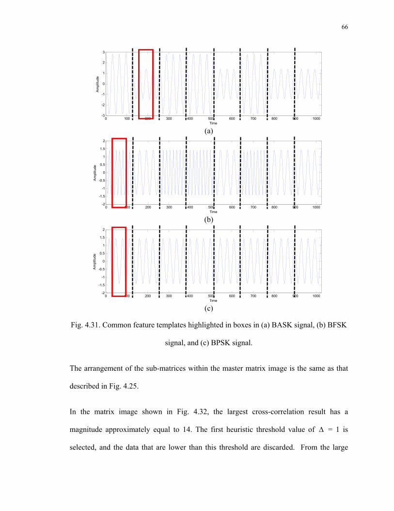
66
0 100 200 300 400 500 600 700 800 900 1000-3
-2
-1
0
1
2
3
Time
Am
plitu
de
(a)
0 100 200 300 400 500 600 700 800 900 1000-2
-1.5
-1
-0.5
0
0.5
1
1.5
2
Time
Am
plitu
de
(b)
0 100 200 300 400 500 600 700 800 900 1000-2
-1.5
-1
-0.5
0
0.5
1
1.5
2
Time
Am
plitu
de
(c)
Fig. 4.31. Common feature templates highlighted in boxes in (a) BASK signal, (b) BFSK
signal, and (c) BPSK signal.
The arrangement of the sub-matrices within the master matrix image is the same as that
described in Fig. 4.25.
In the matrix image shown in Fig. 4.32, the largest cross-correlation result has a
magnitude approximately equal to 14. The first heuristic threshold value of Δ = 1 is
selected, and the data that are lower than this threshold are discarded. From the large

67
number of white spots present in Fig. 4.32, it is seen that most of the data are, in fact,
discarded. Hence, a suitable wavelet can be immediately identified.
The solid circles on the major diagonal of the matrix image indicate the auto-correlation
values of the various templates in the WD that are large in magnitude for all 3 modulation
schemes. The dotted circles indicate the locations of cross-correlation values
corresponding to the same wavelet. It is seen that the values in these locations have been
discarded during thresholding. This implies that the candidate wavelet is not sensitive
enough when templates of common features representing one of the distinct variations,
e.g., amplitude, frequency or phase, based on the candidate wavelet are cross-correlated
with templates corresponding to any of the other distinctive features using the same
wavelet. It is observed that the most suitable wavelet to be utilized in the WD AMR
process is once again the rbio1.3 wavelet. This is the same wavelet identified in the case
of the unique features templates as described in Section 4.4.1.

68
Fig. 4.32. Matrix image based on the common features templates, with a threshold value
of Δ = 1.
4.5 Discussion of Methodologies
In this chapter, three important preliminary steps have been described that are required
for the development of the WD AMR process.
The first step is the definition of WD templates based on the features contained within a
binary digitally modulated communications signal. Specifically, two categories of
templates are defined for each modulation scheme: unique features templates and
common features templates.
For higher-order modulation schemes, it is must be noted that the number of unique
feature templates that are required for AMR can be very large. This is due to the fact that
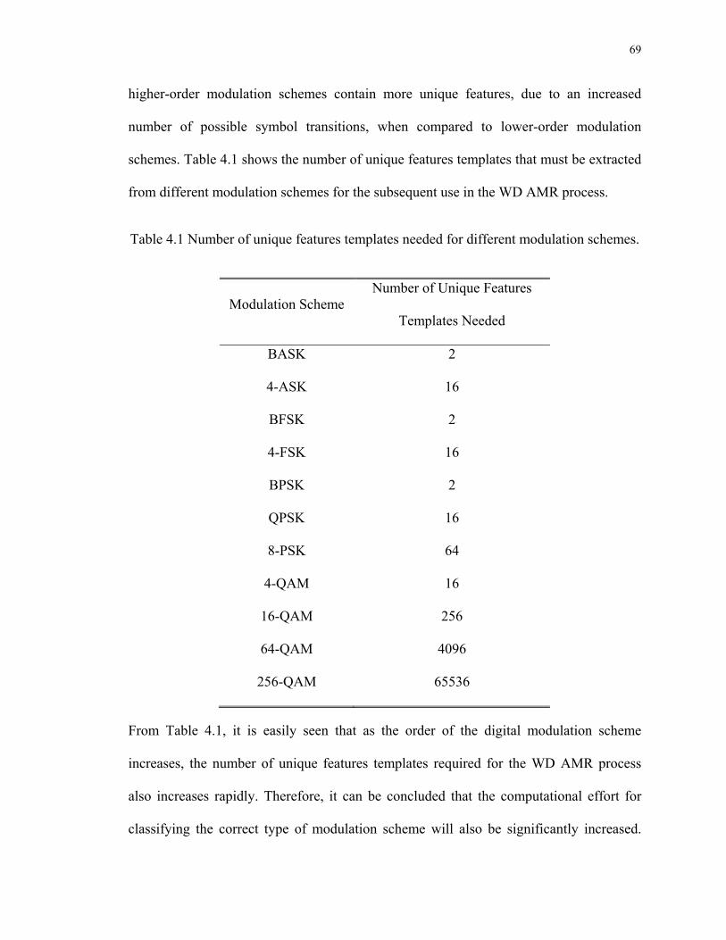
69
higher-order modulation schemes contain more unique features, due to an increased
number of possible symbol transitions, when compared to lower-order modulation
schemes. Table 4.1 shows the number of unique features templates that must be extracted
from different modulation schemes for the subsequent use in the WD AMR process.
Table 4.1 Number of unique features templates needed for different modulation schemes.
Modulation Scheme Number of Unique Features
Templates Needed
BASK 2
4-ASK 16
BFSK 2
4-FSK 16
BPSK 2
QPSK 16
8-PSK 64
4-QAM 16
16-QAM 256
64-QAM 4096
256-QAM 65536
From Table 4.1, it is easily seen that as the order of the digital modulation scheme
increases, the number of unique features templates required for the WD AMR process
also increases rapidly. Therefore, it can be concluded that the computational effort for
classifying the correct type of modulation scheme will also be significantly increased.

70
Due to this observation, the unique features templates will only be used for developing a
WD AMR process for classifying binary digitally modulated communications signals.
On the other hand, the common features templates do not suffer from such a disadvantage
because a minimum of 2 templates to a maximum of only 28 templates are needed to
adequately represent all of the digital modulation schemes considered in this study. The
common features templates are, therefore, used to develop a WD AMR process for all of
the modulation schemes listed in Table 4.1.
In the second preliminary step, WD templates having lengths of 32, 64, and 128 samples
were studied. As shown in Figs. 4.22-4.24, it was observed that those templates
composed of 64 and 128 samples demonstrate stronger cross-correlation results between
the templates and the test communications signals. Due to this observation, the WD
templates that are 32 samples in length are discarded. Therefore, templates that are either
64, or 128 samples in length can be used in developing the WD AMR process since such
templates produce the required resolution in the WD cross-correlation operations. It will
be seen in Chapters 5 and 6 that using templates that are 2N samples in length is
sufficient for very high correct classification rates to be achieved by the AMR process.
Here, N is the number of samples in each signal segment that represents a data symbol.
This is also the case in WD Demodulation, which is described in Chapter 7.
In the third, and final, preliminary step, matrix images that contain the cross-correlation
results of WD templates for BASK, BFSK, and BPSK signals, based on different
wavelets, were created. Two studies were conducted: one using the unique features
templates and the other using the common features templates. On subjecting the data in
71
the matrix images to hard-thresholding with different heuristic threshold values, it has
been found that the most suitable wavelet for developing the WD AMR process is the
rbio1.3 wavelet.
In Chapters 5 and 6, two fundamental WD AMR algorithms are developed, using the rbio
1.3 wavelet, based on the unique features templates and the common features templates,
respectively.
72
Chapter 5
Automatic Modulation Recognition Process Using Unique
Features Templates
AMR can be described as blind identification of the modulation scheme used to format
digital data embedded in a received signal. In this dissertation, the main focus is on
developing a methodology for AMR using WTs in conjunction with pattern recognition.
The WD AMR method employs the concept of template matching for modulation
identification prior to signal demodulation in order to recover the original data bit
sequences over a wide range of SNR values.
The WD AMR process described in this chapter involves the use of unique features
templates that have been developed in Chapter 4. The unique features templates represent
signal features that distinguish the transitions from data symbol ‘0’ to data symbol ‘1’
and vice versa. The transitions are indicated by a change in the amplitude, frequency
and/or phase of a digitally modulated signal. It was identified in Chapter 4 that this set of
templates is suitable for blind identification of binary digitally modulated
communications signals acquired by a communications receiver. The specific modulation
schemes considered here are BASK, BFSK, and BPSK.
5.1 Development of the Automatic Modulation Recognition Process
Using Unique Features Templates
Prior to developing the WD AMR process using unique features templates, the templates
and the wavelet were identified. As demonstrated in Chapter 4, the rbio1.3 wavelet has

73
been identified as the most suitable wavelet for the extraction of both the unique features
and the common features templates. In this chapter, the focus is on the development of a
WD AMR process that makes use of the unique features templates for binary
communications signal since large numbers of unique features templates are required in
the case of higher-order digitally modulated communications signals.
Each of the binary digitally modulated signals considered in this dissertation require two
unique features templates, which are expressed in the WD and are based on the symbol
transitions that are present within a signal. Unique features templates, in both time- and
wavelet-domains, are illustrated graphically in Figs. 5.1-5.3. There are a total of six
unique features templates needed to represent all three binary digital modulation
schemes.
0 10 20 30 40 50 60 70-3
-2
-1
0
1
2
3
Time
Am
plitu
de
(a)
0 10 20 30 40 50 60 70-3
-2
-1
0
1
2
3
Time
Am
plitu
de
(b)
Values of Ca,b Coefficients for a = 1 2 3 4 5 ...
time (or space) b
scal
es a
10 20 30 40 50 60 1 8 15 22 29 36 43 50 57 64 71 78 85 92 99106113120127
(c)
Values of Ca,b Coefficients for a = 1 2 3 4 5 ...
time (or space) b
scal
es a
10 20 30 40 50 60 1 8 15 22 29 36 43 50 57 64 71 78 85 92 99106113120127
(d)
Fig. 5.1. Unique features templates for BASK signal (a-b) in time-domain, (c-d) in
wavelet-domain.
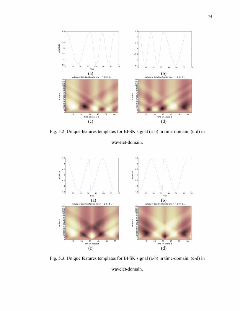
74
0 10 20 30 40 50 60 70-1.5
-1
-0.5
0
0.5
1
1.5
Am
plitu
de
Time
(a) 0 10 20 30 40 50 60 70
-1.5
-1
-0.5
0
0.5
1
1.5
(b) Values of Ca,b Coefficients for a = 1 2 3 4 5 ...
time (or space) b
scal
es a
10 20 30 40 50 60 1 8 15 22 29 36 43 50 57 64 71 78 85 92 99106113120127
(c)
Values of Ca,b Coefficients for a = 1 2 3 4 5 ...
time (or space) b
scal
es a
10 20 30 40 50 60 1 8 15 22 29 36 43 50 57 64 71 78 85 92 99106113120127
(d)
Fig. 5.2. Unique features templates for BFSK signal (a-b) in time-domain, (c-d) in
wavelet-domain.
0 10 20 30 40 50 60 70-1.5
-1
-0.5
0
0.5
1
1.5
Time
Am
plitu
de
(a)
0 10 20 30 40 50 60 70-1.5
-1
-0.5
0
0.5
1
1.5
Time
Am
plitu
de
(b)
Values of Ca,b Coefficients for a = 1 2 3 4 5 ...
time (or space) b
scal
es a
10 20 30 40 50 60 1 8 15 22 29 36 43 50 57 64 71 78 85 92 99106113120127
(c)
Values of Ca,b Coefficients for a = 1 2 3 4 5 ...
time (or space) b
scal
es a
10 20 30 40 50 60 1 8 15 22 29 36 43 50 57 64 71 78 85 92 99106113120127
(d)
Fig. 5.3. Unique features templates for BPSK signal (a-b) in time-domain, (c-d) in
wavelet-domain.
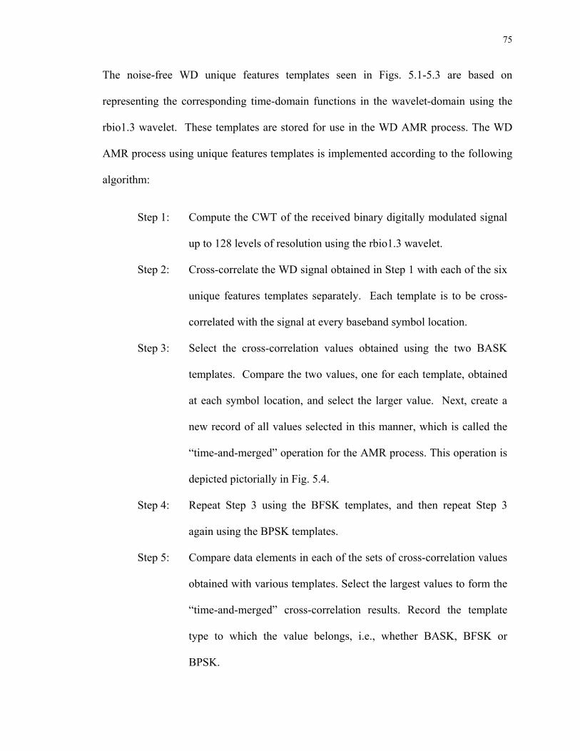
75
The noise-free WD unique features templates seen in Figs. 5.1-5.3 are based on
representing the corresponding time-domain functions in the wavelet-domain using the
rbio1.3 wavelet. These templates are stored for use in the WD AMR process. The WD
AMR process using unique features templates is implemented according to the following
algorithm:
Step 1: Compute the CWT of the received binary digitally modulated signal
up to 128 levels of resolution using the rbio1.3 wavelet.
Step 2: Cross-correlate the WD signal obtained in Step 1 with each of the six
unique features templates separately. Each template is to be cross-
correlated with the signal at every baseband symbol location.
Step 3: Select the cross-correlation values obtained using the two BASK
templates. Compare the two values, one for each template, obtained
at each symbol location, and select the larger value. Next, create a
new record of all values selected in this manner, which is called the
“time-and-merged” operation for the AMR process. This operation is
depicted pictorially in Fig. 5.4.
Step 4: Repeat Step 3 using the BFSK templates, and then repeat Step 3
again using the BPSK templates.
Step 5: Compare data elements in each of the sets of cross-correlation values
obtained with various templates. Select the largest values to form the
“time-and-merged” cross-correlation results. Record the template
type to which the value belongs, i.e., whether BASK, BFSK or
BPSK.
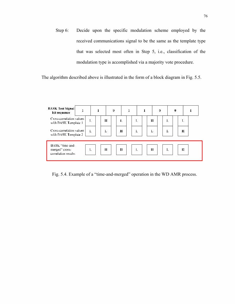
76
Step 6: Decide upon the specific modulation scheme employed by the
received communications signal to be the same as the template type
that was selected most often in Step 5, i.e., classification of the
modulation type is accomplished via a majority vote procedure.
The algorithm described above is illustrated in the form of a block diagram in Fig. 5.5.
Fig. 5.4. Example of a “time-and-merged” operation in the WD AMR process.
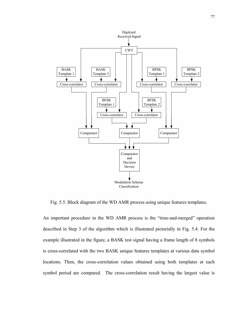
77
CWT
Cross-correlator
BASK Template 1
Cross-correlator
BASK Template 2
Cross-correlator
BFSK Template 1
Cross-correlator
BFSK Template 2
Cross-correlator
BPSK Template 1
Cross-correlator
BPSK Template 2
ComparatorComparator
Comparatorand
Decision Device
Comparator
DigitizedReceived Signal
Modulation Scheme Classification
Fig. 5.5. Block diagram of the WD AMR process using unique features templates.
An important procedure in the WD AMR process is the “time-and-merged” operation
described in Step 3 of the algorithm which is illustrated pictorially in Fig. 5.4. For the
example illustrated in the figure, a BASK test signal having a frame length of 8 symbols
is cross-correlated with the two BASK unique features templates at various data symbol
locations. Then, the cross-correlation values obtained using both templates at each
symbol period are compared. The cross-correlation result having the largest value is
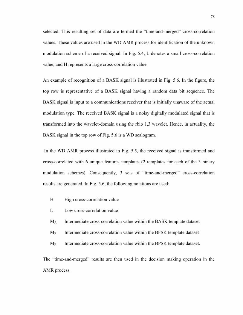
78
selected. This resulting set of data are termed the “time-and-merged” cross-correlation
values. These values are used in the WD AMR process for identification of the unknown
modulation scheme of a received signal. In Fig. 5.4, L denotes a small cross-correlation
value, and H represents a large cross-correlation value.
An example of recognition of a BASK signal is illustrated in Fig. 5.6. In the figure, the
top row is representative of a BASK signal having a random data bit sequence. The
BASK signal is input to a communications receiver that is initially unaware of the actual
modulation type. The received BASK signal is a noisy digitally modulated signal that is
transformed into the wavelet-domain using the rbio 1.3 wavelet. Hence, in actuality, the
BASK signal in the top row of Fig. 5.6 is a WD scalogram.
In the WD AMR process illustrated in Fig. 5.5, the received signal is transformed and
cross-correlated with 6 unique features templates (2 templates for each of the 3 binary
modulation schemes). Consequently, 3 sets of “time-and-merged” cross-correlation
results are generated. In Fig. 5.6, the following notations are used:
H High cross-correlation value
L Low cross-correlation value
MA Intermediate cross-correlation value within the BASK template dataset
MF Intermediate cross-correlation value within the BFSK template dataset
MP Intermediate cross-correlation value within the BPSK template dataset.
The “time-and-merged” results are then used in the decision making operation in the
AMR process.

79
Fig. 5.6. Example of WD AMR process using the unique features templates.
The “time-and-merged” results for the example are highlighted in the box shown in Fig.
5.6. For each symbol period, the three “time-and-merged” data results are compared. The
template having the best match to a candidate modulation type is identified based on the
largest value contained in the “time-and-merged” data. The classification of the unknown
modulation scheme is then accomplished via a majority vote of all the element-wise
template identifications previously made. In the example of Fig. 5.6, BASK templates are

80
identified as being present in the received signal most often. Therefore, the modulation
scheme employed by the received test signal is recognized to be that of BASK.
5.2 Simulation Experiment and Results
All of the binary digitally modulated test signals used in this study have been corrupted
by zero-mean AWGN during transmission to produce received signals with SNR values
in the range of -5 dB to 10 dB. The rates of correct classification produced by the WD
AMR algorithm based on the unique features templates have been obtained using 20,000
Monte Carlo trials, where each simulation experiment employs 50 bits per frame. Each
test signal used in the 20,000 trials randomly employs one among the BASK, BFSK, or
BPSK modulation schemes.
The signals are oversampled by a factor of sixteen over the Nyquist rate corresponding to
the carrier frequency. Oversampling is used because more signal content can be
represented in the WD scalogram, which can then enhance the WD AMR process. Perfect
symbol timing with no timing offset is also assumed throughout this dissertation.
All simulations have been performed using MATLAB. The results of the simulations are
provided in Tables 5.1-5.4, which contain the rates of correct classification of signals
with unknown modulation schemes corrupted by AWGN resulting in SNR values of 10
dB, 5 dB, 0 dB, and -5 dB.
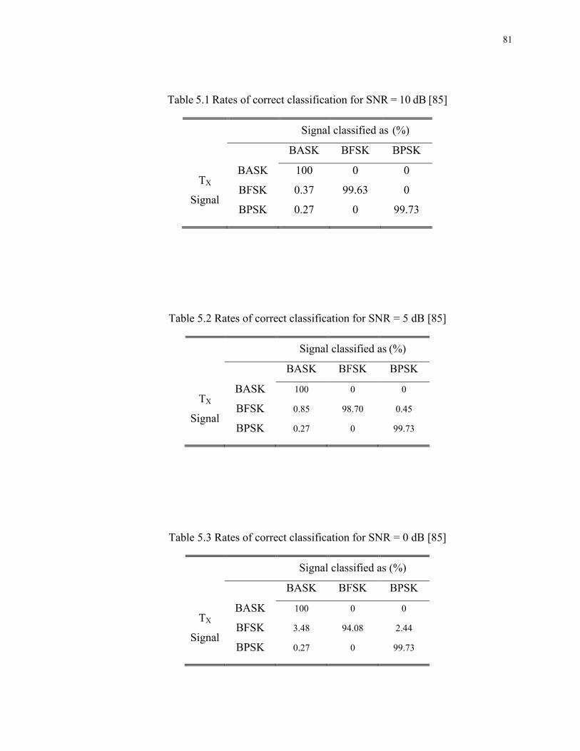
81
Table 5.1 Rates of correct classification for SNR = 10 dB [85]
Signal classified as (%)
BASK BFSK BPSK
TX
Signal
BASK 100 0 0
BFSK 0.37 99.63 0
BPSK 0.27 0 99.73
Table 5.2 Rates of correct classification for SNR = 5 dB [85]
Signal classified as (%)
BASK BFSK BPSK
TX
Signal
BASK 100 0 0
BFSK 0.85 98.70 0.45
BPSK 0.27 0 99.73
Table 5.3 Rates of correct classification for SNR = 0 dB [85]
Signal classified as (%)
BASK BFSK BPSK
TX
Signal
BASK 100 0 0
BFSK 3.48 94.08 2.44
BPSK 0.27 0 99.73
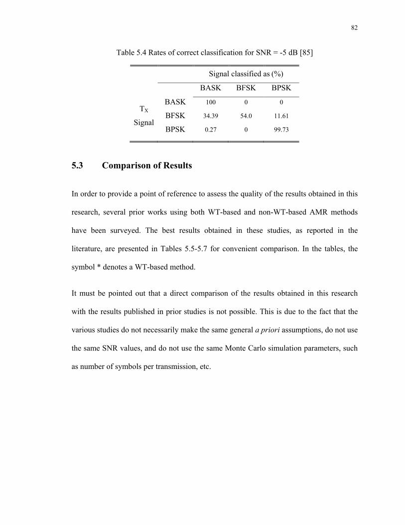
82
Table 5.4 Rates of correct classification for SNR = -5 dB [85]
Signal classified as (%)
BASK BFSK BPSK
TX
Signal
BASK 100 0 0
BFSK 34.39 54.0 11.61
BPSK 0.27 0 99.73
5.3 Comparison of Results
In order to provide a point of reference to assess the quality of the results obtained in this
research, several prior works using both WT-based and non-WT-based AMR methods
have been surveyed. The best results obtained in these studies, as reported in the
literature, are presented in Tables 5.5-5.7 for convenient comparison. In the tables, the
symbol * denotes a WT-based method.
It must be pointed out that a direct comparison of the results obtained in this research
with the results published in prior studies is not possible. This is due to the fact that the
various studies do not necessarily make the same general a priori assumptions, do not use
the same SNR values, and do not use the same Monte Carlo simulation parameters, such
as number of symbols per transmission, etc.
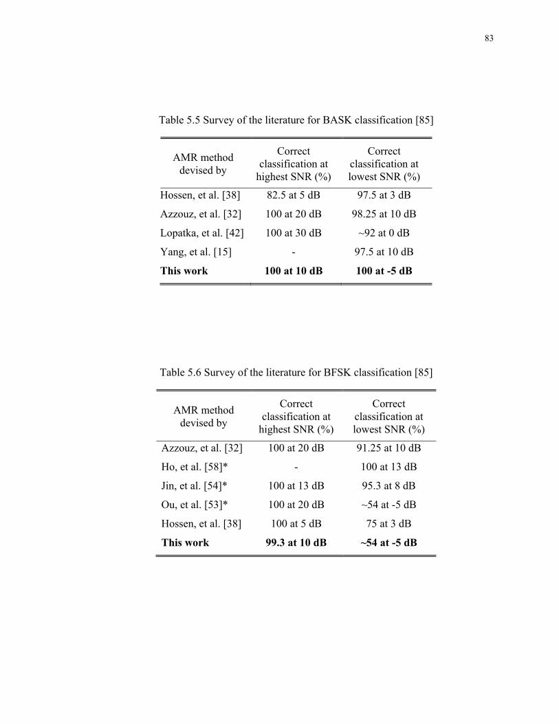
83
Table 5.5 Survey of the literature for BASK classification [85]
AMR method devised by
Correct classification at
highest SNR (%)
Correct classification at lowest SNR (%)
Hossen, et al. [38] 82.5 at 5 dB 97.5 at 3 dB
Azzouz, et al. [32] 100 at 20 dB 98.25 at 10 dB
Lopatka, et al. [42] 100 at 30 dB ~92 at 0 dB
Yang, et al. [15] - 97.5 at 10 dB
This work 100 at 10 dB 100 at -5 dB
Table 5.6 Survey of the literature for BFSK classification [85]
AMR method devised by
Correct classification at
highest SNR (%)
Correct classification at lowest SNR (%)
Azzouz, et al. [32] 100 at 20 dB 91.25 at 10 dB
Ho, et al. [58]* - 100 at 13 dB
Jin, et al. [54]* 100 at 13 dB 95.3 at 8 dB
Ou, et al. [53]* 100 at 20 dB ~54 at -5 dB
Hossen, et al. [38] 100 at 5 dB 75 at 3 dB
This work 99.3 at 10 dB ~54 at -5 dB

84
Table 5.7 Survey of the literature for BPSK classification [85]
AMR method devised by
Correct classification at
highest SNR (%)
Correct classification at lowest SNR (%)
Azzouz, et al. [32] 90.75 at 20 dB 96.25 at 10 dB
Dobre, et al. [9] - 100 at 2 dB
Ho, et al. [58]* - 98 at 13 dB
Jin, et al. [54]* 100 at 13 dB 99.5 at 8 dB
Ou, et al. [53]* 100 at 20 dB ~54 at -5 dB
Hossen, et al. [38] 100 at 5dB 87.5 at 3dB
This work 99.7 at 10 dB 99.7 at -5 dB
Two prior WT-based AMR studies involve computing the histogram of the CWT
coefficients of the received signals and then counting the number of peaks in the
histogram in order to classify the received signal as either BPSK or BFSK [53], [58]. The
rates of correct classification for BPSK signals is 98% and for BFSK signals is 100% at
an SNR = 13 dB in [58]. For the classification rates reported in [53], both BPSK and
BFSK modulation were recognized at a rate of 100% at SNR = 20 dB. However, a rate of
only 54% was achieved at SNR = -5 dB for both modulation types. In this work, the rates
of correct classification are 100%, 99.3%, and 99.7% at SNR = 10 dB, for BASK, BFSK
and BPSK signals, respectively. In the case of SNR = -5 dB, the rates of correct
classification are 100% for BASK signals, 54% for BFSK signals, and 99.7% for BPSK
signals.

85
5.4 Conclusions
It is observed from Tables 5.5-5.7 that the rates of correct classification of binary
digitally modulated signals realized by the WD AMR process are equal to or better than
the rates reported in the literature, especially when compared the WT-based AMR
methods.
It has been determined via extensive computer simulations that the rate of correct
classification for BASK signals is 100% and for BPSK signals the rate is 99.7% over the
range of SNR values considered. The rates of correct classification for BFSK signals are
99.6%, 98.7%, 94.0% and 54% for SNR = 10 dB, 5 dB, 0 dB and -5 dB, respectively.
For the WD AMR process devised in this chapter, there are two important procedural
factors that might have a substantial impact on the performance of the AMR process.
The first factor affecting the AMR performance is the number of baseband data symbols
that comprise each transmitted signal. As described in Section 5.1, classification of
unknown modulation schemes is accomplished based on the “time-and-merged” cross-
correlation data via majority vote. Due to this procedure, it is reasonable that longer
baseband data symbol sequences in each transmission interval, or frame, may provide
better classification rates. Conversely, baseband data sequences of reduced lengths could
result in poorer rates of correct classification than those obtained in this study. This
hypothesis has been tested using computer simulations. The results reported in Table 5.8
show the rates of correct classification for BPSK signals having baseband symbol
sequences of different lengths. The signals have been corrupted by AWGN such that
SNR = 0 dB. These results confirm the prediction in that lower rates of correct

86
classification are obtained with WD AMR using the unique features templates consisting
of baseband symbol sequences of shorter length.
Table 5.8 Rates of correct classification for different baseband symbol sequence lengths
using BPSK signals
Length of the data words (bits) Correct classification rate at 0 dB
50 99.73%
20 94.34%
10 82.56%
The second factor affecting the performance of the WD AMR process is the choice of
wavelet used. After computing the cross-correlation matrix for the unique features
templates using 65 different wavelets in order to determine the suitable wavelet(s) in
Chapter 4, it was observed that certain wavelets are more sensitive to the unique features
of a particular modulation schemes compared to other modulation schemes. This
observation raises the possibility that better rates of classification for BFSK signals than
those obtained in this study might be attainable using a different wavelet. The choice of
wavelet is determined based on the techniques devised in Chapter 4. From the matrix in
Fig. 4.29, the center sub-matrix represents the cross-correlation values of BFSK
templates expressed in 65 different versions. It is observed that the darker spots within
the sub-matrix show larger cross-correlation value. Some of darker spots only occur
within the sub-matrix, therefore, these spots, which correspond to specific wavelets, can
possibly be used to develop an WD AMR procedure to improve the classification rates
87
for BFSK signals. This is due to the sensitivity of the specific wavelet to the modulation
characteristics contained within a communications signal.
88
Chapter 6
Automatic Modulation Recognition Process Using Common
Features Templates
The AMR algorithm developed in this chapter is based on the common features templates
that have been constructed in the WD. The detailed procedure for the construction of the
templates has been provided in Chapter 4. The templates are used in the cross-correlation
operations within the AMR process to obtain decision variables. The digitally modulated
signals considered in this chapter include M-ary ASK and M-ary FSK for M = 2 and 4;
MPSK for M = 2, 4, and 8; and M-ary QAM for M = 4, 16, 64, and 256. The
communications signals are corrupted with AWGN in the range of SNR from -5 dB to 10
dB.
In Section 6.1, several preliminary methodologies required for the WD AMR process
using the common features templates are described. The WD AMR algorithm is then
developed in Section 6.2. The WD AMR process is verified and evaluated. The results
are presented in Section 6.3. Comparisons of the rates of correct modulation classification
obtained in this study are made with results found in the literature. The comparisons are
presented in Section 6.4.
6.1 Development of the Automatic Modulation Recognition Process
Using Common Features Templates
As described in Chapter 5, the communications signal is first transformed into the WD
using the CWT. The resulting CWT expression of the signal is then cross-correlated with
89
templates representing WD signatures of the candidate modulated signals. In this second
WD AMR algorithm developed within this dissertation, the common features templates
are used. Whereas, the unique features templates were used in the WD AMR algorithm
presented in Chapter 5.
Recall from Chapter 4, that the common features templates are constructed based on the
sinusoidal feature inherent in all of the digitally modulated communications signals
considered in this study. In general, the sinusoidal feature is defined as
( ) ( )cos 2 cs t f tπ= (6.1)
where fc is used to denoted the carrier frequency of the signal.
As mentioned in both Chapters 3 and 4, the sinusoidal features can be extracted at
different temporal locations within a data symbol period of a communications signal. A
common features template can also be subjected to a time-shift, which would correspond
to a phase shift of the carrier signal. Therefore, in general, a common features template,
( )p t , can be defined as
( ) ( ) 1 2cos 2 cp t f t T t Tπ θ= + < < (6.2)
where θ represents the different phase shifts of the sinusoidal carrier, while 1T and 2T
represent the beginning time and ending time of the template.
It has also been noted in Chapter 4 that temporal shifts of a signal in the time-domain
correspond exactly to shifts indicated by the translation variable, b, in the wavelet-
domain. Therefore, the phase-shifting operation in the time-domain has the time-shift
effect that is desired in the wavelet-domain.
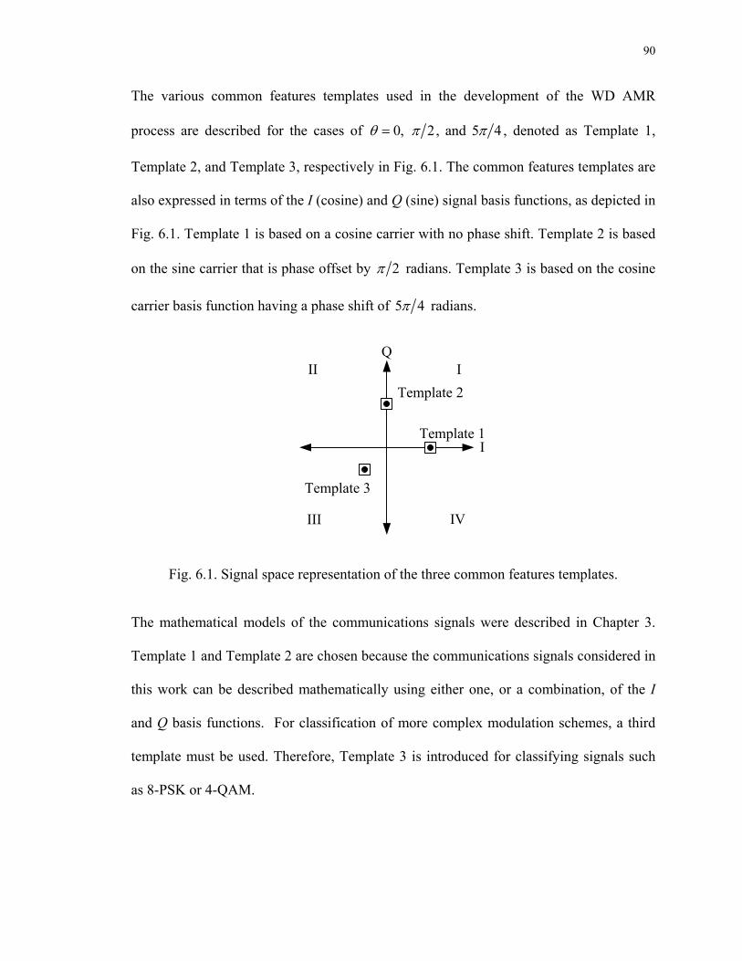
90
The various common features templates used in the development of the WD AMR
process are described for the cases of 0, 2, and 5 4θ π π= , denoted as Template 1,
Template 2, and Template 3, respectively in Fig. 6.1. The common features templates are
also expressed in terms of the I (cosine) and Q (sine) signal basis functions, as depicted in
Fig. 6.1. Template 1 is based on a cosine carrier with no phase shift. Template 2 is based
on the sine carrier that is phase offset by 2π radians. Template 3 is based on the cosine
carrier basis function having a phase shift of 5 4π radians.
I
Q
Template 1
Template 2
Template 3
III
III IV
Fig. 6.1. Signal space representation of the three common features templates.
The mathematical models of the communications signals were described in Chapter 3.
Template 1 and Template 2 are chosen because the communications signals considered in
this work can be described mathematically using either one, or a combination, of the I
and Q basis functions. For classification of more complex modulation schemes, a third
template must be used. Therefore, Template 3 is introduced for classifying signals such
as 8-PSK or 4-QAM.

91
The WD scalograms of the three common feature templates, T1, T2 and T3, are illustrated
in Fig. 6.2.
In Fig. 6.2 (a) the wavelet-domain representation for Template 1 of a sinusoidal carrier of
finite duration with no phase shift is illustrated. The WD representation for Template 2
consisting of a phase shift of 2π radians is shown in Fig. 6.2 (b). Fig. 6.2 (c) illustrates
the WD representation for Template 3 corresponding to a sinusoidal carrier with a phase
shift of 5 4π radians.
(a) 0θ =
(b) 2θ π=
(c) 5 4θ π=
Fig. 6.2. The three common features templates used for the AMR process.
In developing the WD AMR algorithm, the cross-correlation values between the
templates and the signal are first investigated. A sinusoidal function having phase shifts
in increments of 10o is cross-correlated with Template 1 and Template 2. The signals
with different phase shifts can be expressed in term of a signal constellation along a unit
circle. Several observations are made based on the cross-correlation values with such
sinusoidal signals and the templates.
The cross-correlation results obtained for Template 1 and Template 2 when compared to
several sinusoidal functions are computed. The cross-correlation data involving Template
1 and Template 2 are tabulated in Tables 6.1 and 6.2, respectively. The first observation
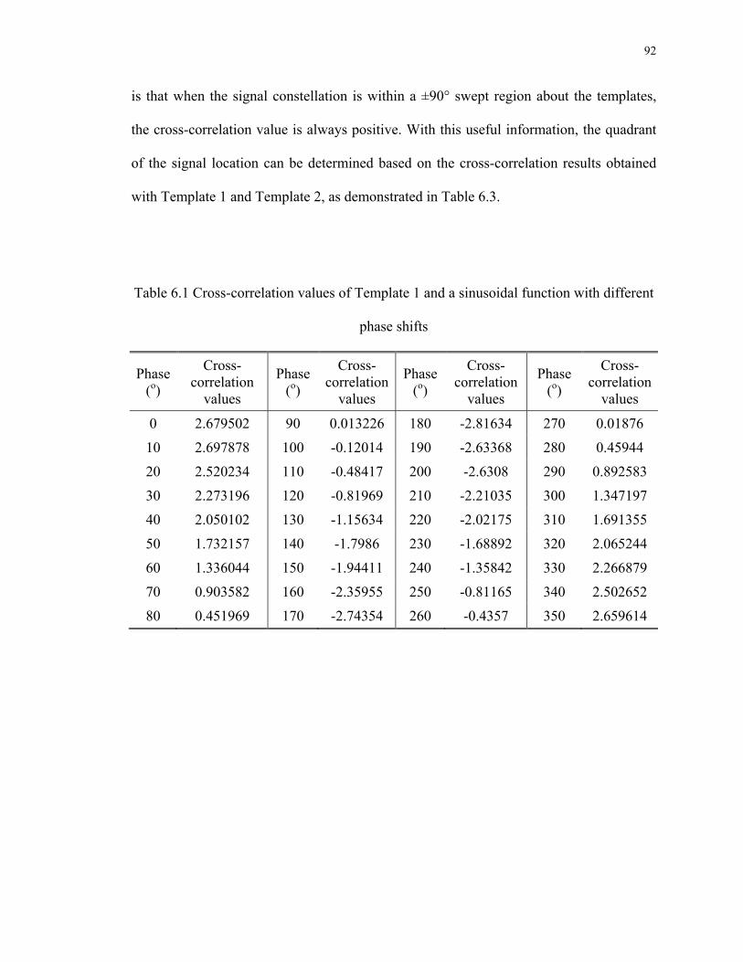
92
is that when the signal constellation is within a ±90° swept region about the templates,
the cross-correlation value is always positive. With this useful information, the quadrant
of the signal location can be determined based on the cross-correlation results obtained
with Template 1 and Template 2, as demonstrated in Table 6.3.
Table 6.1 Cross-correlation values of Template 1 and a sinusoidal function with different
phase shifts
Phase (o)
Cross-correlation
values
Phase (o)
Cross-correlation
values
Phase (o)
Cross-correlation
values
Phase (o)
Cross-correlation
values
0 2.679502 90 0.013226 180 -2.81634 270 0.01876
10 2.697878 100 -0.12014 190 -2.63368 280 0.45944
20 2.520234 110 -0.48417 200 -2.6308 290 0.892583
30 2.273196 120 -0.81969 210 -2.21035 300 1.347197
40 2.050102 130 -1.15634 220 -2.02175 310 1.691355
50 1.732157 140 -1.7986 230 -1.68892 320 2.065244
60 1.336044 150 -1.94411 240 -1.35842 330 2.266879
70 0.903582 160 -2.35955 250 -0.81165 340 2.502652
80 0.451969 170 -2.74354 260 -0.4357 350 2.659614

93
Table 6.2 Cross-correlation values of Template 2 and a sinusoidal function with different
phase shifts
Phase (o)
Cross-correlation
values
Phase (o)
Cross-correlation
values
Phase (o)
Cross-correlation
values
Phase (o)
Cross-correlation
values
0 0.00129 90 2.815686 180 -0.09995 270 -2.70652
10 0.34639 100 2.503755 190 -0.57392 280 -2.52334
20 0.889756 110 2.255107 200 -0.82939 290 -2.4098
30 1.306933 120 2.066662 210 -1.30233 300 -2.11353
40 1.916086 130 1.799082 220 -1.68042 310 -1.86032
50 2.088706 140 1.505474 230 -1.98736 320 -1.46584
60 2.210679 150 0.901692 240 -2.24363 330 -0.77707
70 2.619054 160 0.386802 250 -2.60393 340 -0.35054
80 2.706011 170 0.088836 260 -2.62592 350 -0.11447
Table 6.3 Identification of signal space quadrant using the cross-correlation results of
Template 1 and Template 2
Quadrant Cross-correlation
with
Template 1
Cross-correlation with
Template 2
I + +
II - +
III - -
IV + -
In Figs. 6.3-6.13, the cross-correlation data obtained using a test signal compared with
each of the three common features templates are plotted. Based on observations about the
characteristics associated with from each set of cross-correlation data, the discrimination
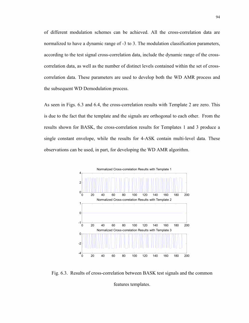
94
of different modulation schemes can be achieved. All the cross-correlation data are
normalized to have a dynamic range of -3 to 3. The modulation classification parameters,
according to the test signal cross-correlation data, include the dynamic range of the cross-
correlation data, as well as the number of distinct levels contained within the set of cross-
correlation data. These parameters are used to develop both the WD AMR process and
the subsequent WD Demodulation process.
As seen in Figs. 6.3 and 6.4, the cross-correlation results with Template 2 are zero. This
is due to the fact that the template and the signals are orthogonal to each other. From the
results shown for BASK, the cross-correlation results for Templates 1 and 3 produce a
single constant envelope, while the results for 4-ASK contain multi-level data. These
observations can be used, in part, for developing the WD AMR algorithm.
0 20 40 60 80 100 120 140 160 180 2000
2
4Normalized Cross-correlation Results with Template 1
0 20 40 60 80 100 120 140 160 180 200-1
0
1Normalized Cross-correlation Results with Template 2
0 20 40 60 80 100 120 140 160 180 200-4
-2
0Normalized Cross-correlation Results with Template 3
Fig. 6.3. Results of cross-correlation between BASK test signals and the common
features templates.

95
0 20 40 60 80 100 120 140 160 180 2000
2
4Normalized Cross-correlation Results with Template 1
0 20 40 60 80 100 120 140 160 180 200-1
0
1Normalized Cross-correlation Results with Template 2
0 20 40 60 80 100 120 140 160 180 200-4
-2
0Normalized Cross-correlation Results with Template 3
Fig. 6.4. Results of cross-correlation between 4-ASK test signals and the common
features templates.
0 20 40 60 80 100 120 140 160 180 2000
2
4Normalized Cross-correlation Results with Template 1
0 20 40 60 80 100 120 140 160 180 200-1
0
1Normalized Cross-correlation Results with Template 2
0 20 40 60 80 100 120 140 160 180 200-4
-2
0Normalized Cross-correlation Results with Template 3
Fig. 6.5. Results of cross-correlation between BFSK test signals and the common features
templates.

96
0 20 40 60 80 100 120 140 160 180 2000
2
4Normalized Cross-correlation Results with Template 1
0 20 40 60 80 100 120 140 160 180 200-1
0
1Normalized Cross-correlation Results with Template 2
0 20 40 60 80 100 120 140 160 180 200-4
-2
0Normalized Cross-correlation Results with Template 3
Fig. 6.6. Results of cross-correlation between 4-FSK test signals and the common
features templates.
In Figs. 6.5 and 6.6, the cross-correlation results for the BFSK and 4-FSK test signals
with all 3 common features templates are shown, respectively. It is seen that plots of the
cross-correlation data obtained using Templates 1 and 3 have constant amplitude
envelopes for both modulation schemes. The results when using Template 2, however,
are zero for both modulation schemes. This is due to the fact that the signal is orthogonal
to the template as noted previously for ASK signals.
Due to the similarity of the correlation results shown for both BFSK and 4-FSK signals,
i.e., the constant envelope for both correlation results with Template 1 and Template 3,
and the zero cross-correlation result with Template 2, it is necessary to introduce
additional templates for use in the WD AMR process.

97
0 20 40 60 80 100 120 140 160 180 200-5
0
5Normalized Cross-correlation Results with Template 1
0 20 40 60 80 100 120 140 160 180 200-1
0
1Normalized Cross-correlation Results with Template 2
0 20 40 60 80 100 120 140 160 180 200-5
0
5Normalized Cross-correlation Results with Template 3
Fig. 6.7. Results of cross-correlation between BPSK test signals and the common features
templates.
The WD cross-correlation values for BPSK, QPSK and 8-PSK signals with all 3 common
features templates are plotted in Figs. 6.7-6.9, respectively. Among the 3 modulation
schemes, only the correlation results for the BPSK test signal with Templates 1 and 3
shows the property of having a constant amplitude envelope, as seen in Fig. 6.7. This
constant envelope property has also been exhibited by the WD cross-correlation values
for the M-ary ASK and M-ary FSK test signals, as seen in Figs. 6.3-6.6.
The difference between these sets of results is the dynamic range of the cross-correlation
values. The dynamic range of the BPSK test signals is that from -3 to 3, while the
dynamic range of the M-ary ASK and M-ary FSK test results is strictly positive between
0 and 3.
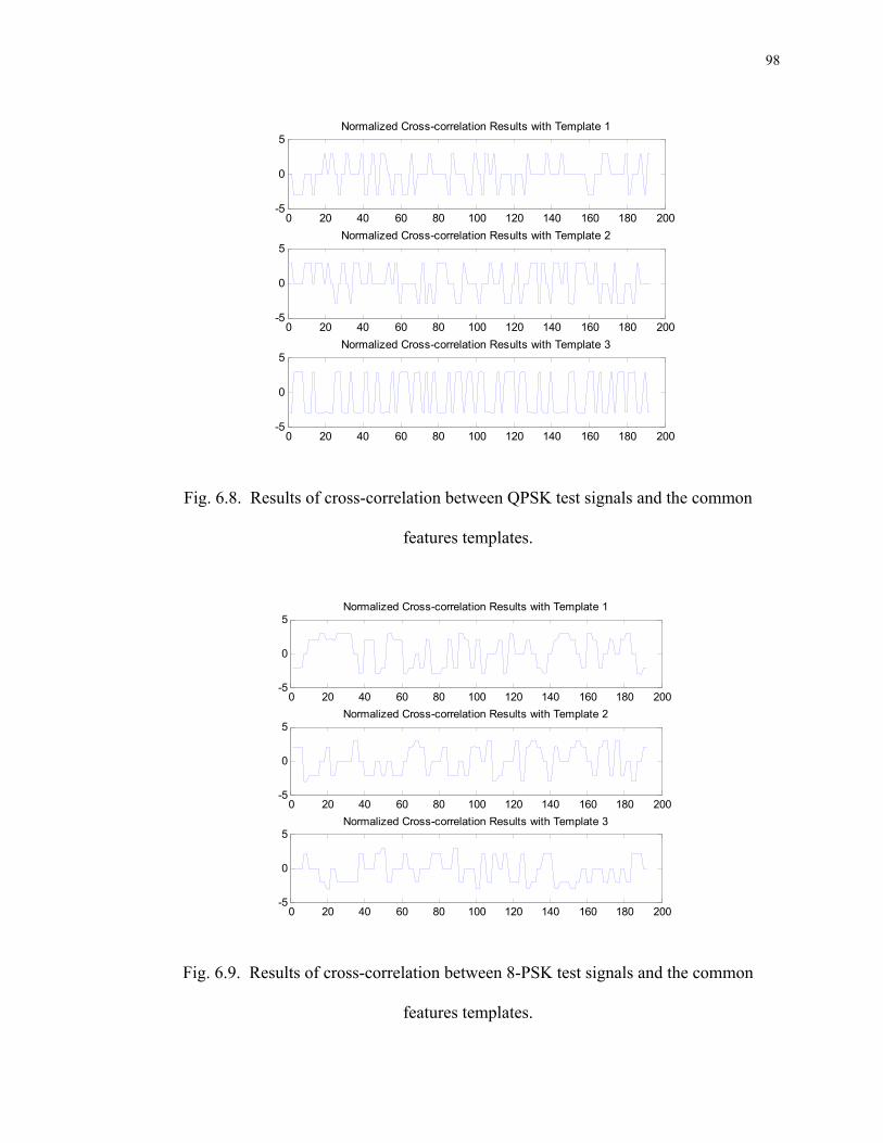
98
0 20 40 60 80 100 120 140 160 180 200-5
0
5Normalized Cross-correlation Results with Template 1
0 20 40 60 80 100 120 140 160 180 200-5
0
5Normalized Cross-correlation Results with Template 2
0 20 40 60 80 100 120 140 160 180 200-5
0
5Normalized Cross-correlation Results with Template 3
Fig. 6.8. Results of cross-correlation between QPSK test signals and the common
features templates.
0 20 40 60 80 100 120 140 160 180 200-5
0
5Normalized Cross-correlation Results with Template 1
0 20 40 60 80 100 120 140 160 180 200-5
0
5Normalized Cross-correlation Results with Template 2
0 20 40 60 80 100 120 140 160 180 200-5
0
5Normalized Cross-correlation Results with Template 3
Fig. 6.9. Results of cross-correlation between 8-PSK test signals and the common
features templates.

99
From Figs. 6.8 and 6.9, it is observed that the WD cross-correlation values of both QPSK
and 8-PSK signals with the 2 common features templates have a dynamic range from -3
to 3. However, the data may cluster into multiple levels within this range. In other words,
the values do not provide constant amplitude envelopes. It is also seen that the WD cross-
correlation results for the 8-PSK test signals when compared with all 3 templates exhibit
multi-level characteristics.
0 20 40 60 80 100 120 140 160 180 200-5
0
5Normalized Cross-correlation Results with Template 1
0 20 40 60 80 100 120 140 160 180 200-5
0
5Normalized Cross-correlation Results with Template 2
0 20 40 60 80 100 120 140 160 180 200-5
0
5Normalized Cross-correlation Results with Template 3
Fig. 6.10. Results of cross-correlation between the 4-QAM ( 4π -QPSK) test signal and
the common features templates.
The results of cross-correlating a 4-QAM ( 4π -QPSK) test signal with the common
features templates are shown in Fig. 6.10. In this case the values obtained with Templates
1 and 2 have numerical values that again form a constant envelope when plotted versus
time. On the other hand, the values obtained when Template 3 is used have 3 different
amplitudes.
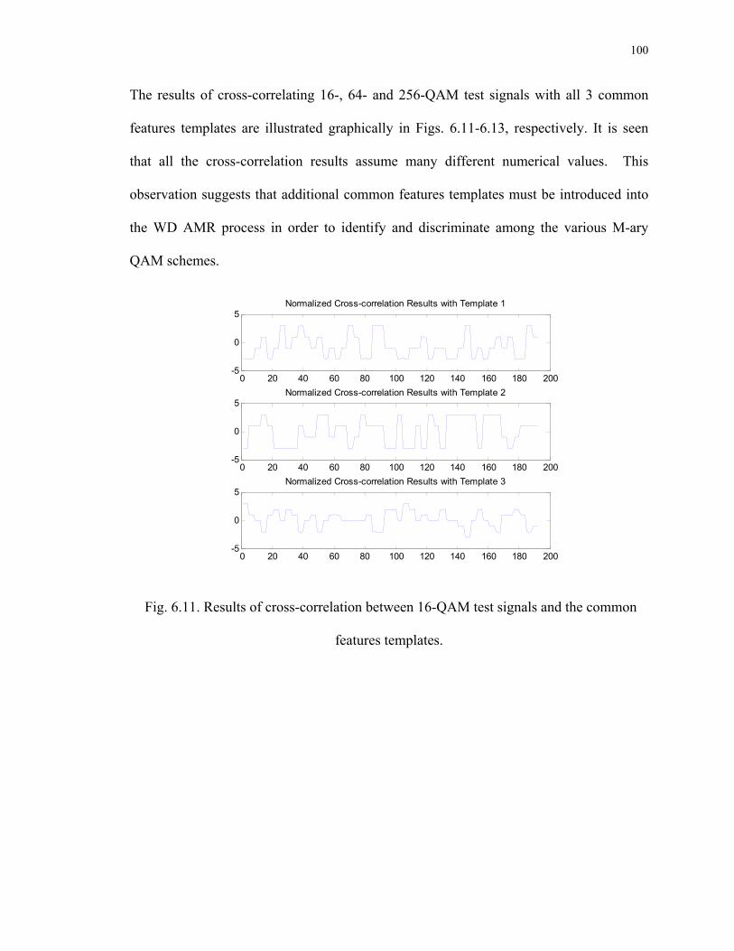
100
The results of cross-correlating 16-, 64- and 256-QAM test signals with all 3 common
features templates are illustrated graphically in Figs. 6.11-6.13, respectively. It is seen
that all the cross-correlation results assume many different numerical values. This
observation suggests that additional common features templates must be introduced into
the WD AMR process in order to identify and discriminate among the various M-ary
QAM schemes.
0 20 40 60 80 100 120 140 160 180 200-5
0
5Normalized Cross-correlation Results with Template 1
0 20 40 60 80 100 120 140 160 180 200-5
0
5Normalized Cross-correlation Results with Template 2
0 20 40 60 80 100 120 140 160 180 200-5
0
5Normalized Cross-correlation Results with Template 3
Fig. 6.11. Results of cross-correlation between 16-QAM test signals and the common
features templates.

101
0 20 40 60 80 100 120 140 160 180 200-5
0
5Normalized Cross-correlation Results with Template 1
0 20 40 60 80 100 120 140 160 180 200-5
0
5Normalized Cross-correlation Results with Template 2
0 20 40 60 80 100 120 140 160 180 200-5
0
5Normalized Cross-correlation Results with Template 3
Fig. 6.12. Results of cross-correlation between 64-QAM test signals and the common
features templates.
0 20 40 60 80 100 120 140 160 180 200-5
0
5Normalized Cross-correlation Results with Template 1
0 20 40 60 80 100 120 140 160 180 200-5
0
5Normalized Cross-correlation Results with Template 2
0 20 40 60 80 100 120 140 160 180 200-5
0
5Normalized Cross-correlation Results with Template 3
Fig. 6.13. Results of cross-correlation between 256-QAM test signals and the common
features templates.
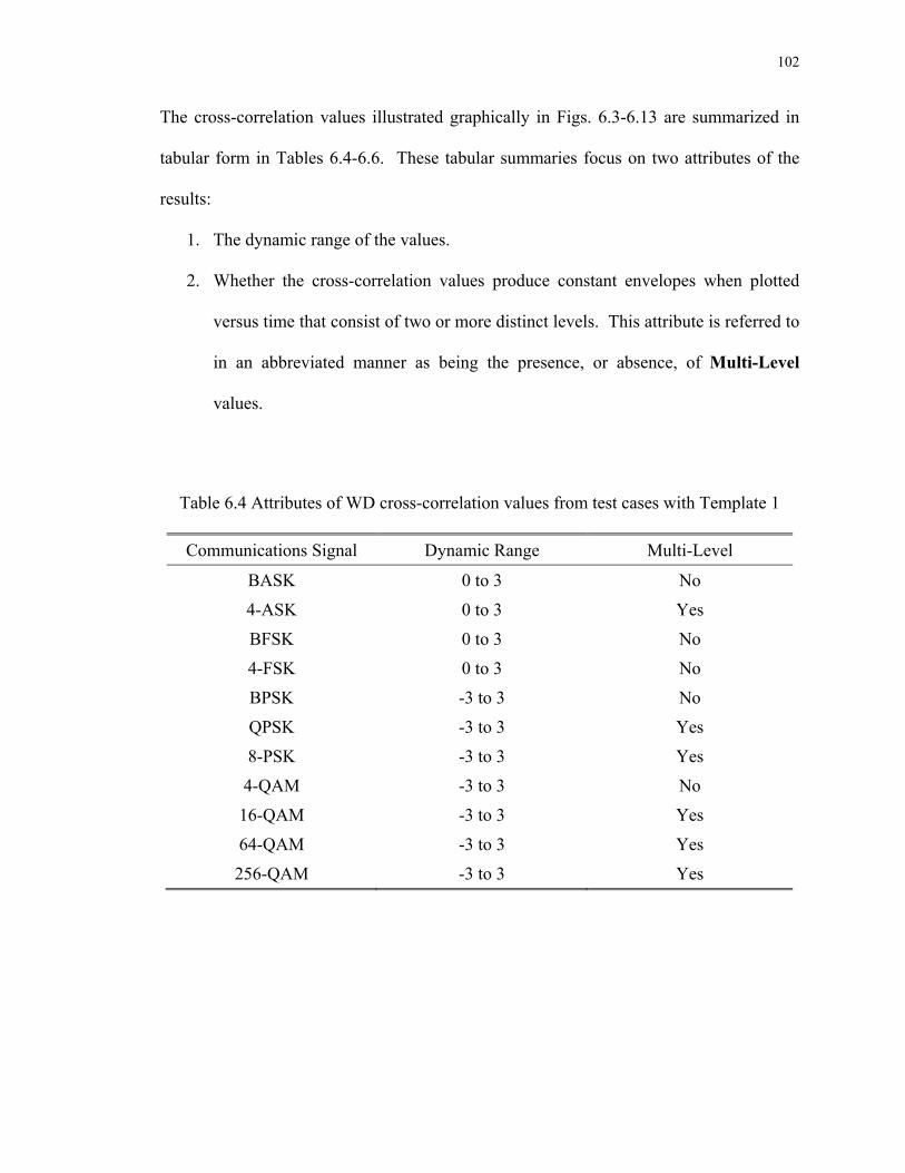
102
The cross-correlation values illustrated graphically in Figs. 6.3-6.13 are summarized in
tabular form in Tables 6.4-6.6. These tabular summaries focus on two attributes of the
results:
1. The dynamic range of the values.
2. Whether the cross-correlation values produce constant envelopes when plotted
versus time that consist of two or more distinct levels. This attribute is referred to
in an abbreviated manner as being the presence, or absence, of Multi-Level
values.
Table 6.4 Attributes of WD cross-correlation values from test cases with Template 1
Communications Signal Dynamic Range Multi-Level
BASK 0 to 3 No
4-ASK 0 to 3 Yes
BFSK 0 to 3 No
4-FSK 0 to 3 No
BPSK -3 to 3 No
QPSK -3 to 3 Yes
8-PSK -3 to 3 Yes
4-QAM -3 to 3 No
16-QAM -3 to 3 Yes
64-QAM -3 to 3 Yes
256-QAM -3 to 3 Yes
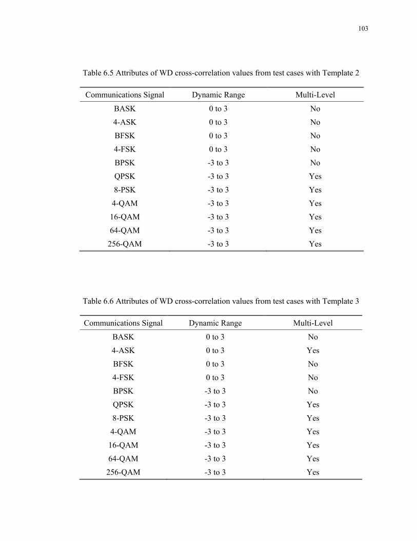
103
Table 6.5 Attributes of WD cross-correlation values from test cases with Template 2
Communications Signal Dynamic Range Multi-Level
BASK 0 to 3 No
4-ASK 0 to 3 No
BFSK 0 to 3 No
4-FSK 0 to 3 No
BPSK -3 to 3 No
QPSK -3 to 3 Yes
8-PSK -3 to 3 Yes
4-QAM -3 to 3 Yes
16-QAM -3 to 3 Yes
64-QAM -3 to 3 Yes
256-QAM -3 to 3 Yes
Table 6.6 Attributes of WD cross-correlation values from test cases with Template 3
Communications Signal Dynamic Range Multi-Level
BASK 0 to 3 No
4-ASK 0 to 3 Yes
BFSK 0 to 3 No
4-FSK 0 to 3 No
BPSK -3 to 3 No
QPSK -3 to 3 Yes
8-PSK -3 to 3 Yes
4-QAM -3 to 3 Yes
16-QAM -3 to 3 Yes
64-QAM -3 to 3 Yes
256-QAM -3 to 3 Yes
104
To summarize the research presented in this section, the concepts used for developing the
WD AMR algorithm using the category of common features templates include:
1. Algebraic sign information from the cross-correlation results obtained with
Templates 1 and 2 leads to identifying the quadrant locations of the symbol within
the signal constellation of a modulation type.
2. Identifying the characteristic combinations of all three template cross-correlation
results, e.g., single-level, multi-level or zero-valued datasets.
6.2 Algorithm for the Automatic Modulation Recognition Process
The general WD AMR process using the common features templates is described by the
following algorithm:
Step 1: The received signal with unknown modulation scheme is transformed using the
CWT employing a rbio1.3 wavelet.
Step 2: The transformed signal is cross-correlated with the common features templates
defined in the wavelet-domain representing the WD signatures.
Step 3: The cross-correlation values are examined and modified in the pre-processing
blocks so as to have a fixed dynamic range.
Step 4: The normalized cross-correlation values are processed by three specific
decision blocks in order for the unknown modulation scheme to be recognized.
The AMR process using the common features templates is illustrated in Fig. 6.14.
The functionality of the pre-processing block operation described in Step 3 of the
algorithm is used to ensure that the cross-correlation data are normalized to have a
105
dynamic range from -3 to 3. After the data have been processed, AMR decision metrics
are developed for each of the decision blocks that are illustrated in Fig. 6.14 in order to
discriminate between different modulation schemes.
The decision blocks are developed based on the attributes of all three sets of cross-
correlation results, i.e., being zero-valued, having numerical values that are multi-level,
or having numerical values that are single-level. Each set of cross-correlation results are
examined using either a dynamic range test (to determine if the range is from -3 to 3, or if
the range is from 0 to 3), or a multi-level test. A combination of three sets of cross-
correlation results is used to classify a particular modulation scheme. The algebraic sign
information from the cross-correlation results obtained Template 1 and Template 2 is
used particularly to classify modulated signals having phase variations between data
symbol transitions.
The development of the various decision block procedures is presented in detail in the
remainder of this section. In particular, Sections 6.2.1-6.2.3 describe the procedures for
Decision Blocks 1, 2 and 3 using the cross-correlation results obtained with Templates 1,
2 and 3. Due to the change of carrier frequencies in FSK signals, additional templates are
introduced for the ASK/FSK Signal Classifier, as described in Section 6.2.4.1. A new
concept called the “moving origin” is introduced in order to classify different orders of
M-ary QAM signals. The PSK/QAM Signal Classifier is described in Section 6.2.4.2.
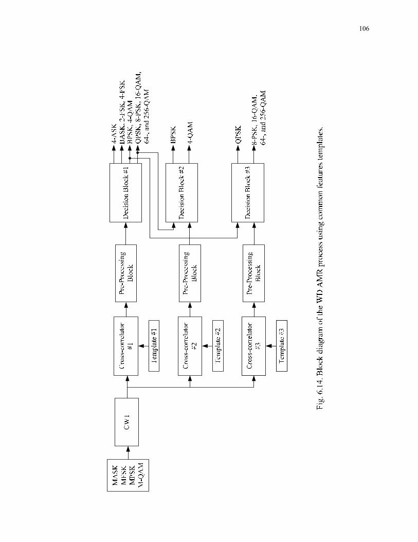
106

107
6.2.1 Procedure for Decision Block 1
From the cross-correlation results in Table 6.4, the modulated signals can be separated
into two groups based on the “dynamic range” attribute of the cross-correlation values
and two other additional groups based on the “multi-level” attribute. Note that the values
obtained using Template 1 are processed in Decision Block 1.
Based on the dynamic range attribute, one group of modulated signals has a dynamic
range that is strictly positive, specifically the range from 0 to 3. The second group of
modulated signals has cross-correlation values in the range from -3 to 3. The two groups
of modulation schemes are specified in Table 6.7.
Table 6.7 Two groups of data identified from Template 1 using dynamic range
Dynamic Range Modulation Schemes
0 to 3 BASK,4-ASK, BFSK, 4-FSK
-3 to 3 BPSK, QPSK, 8-PSK, 4-QAM, 16-QAM, 64-QAM, 256-QAM The second set of groupings is based on whether the cross-correlation values are either
single-level, or multi-level. The groupings of modulation schemes based on this attribute
are specified in Table 6.8.
Table 6.8 Two groups of data identified from Template 1 using multi-level
Multi-Level Modulation Schemes
No BASK, BFSK, 4-FSK, BPSK,4-QAM
Yes 4-ASK, QPSK, 8-PSK,16-QAM, 64-QAM, 256-QAM
Based on the distinct groupings of modulation schemes in Tables 6.7 and 6.8, the
procedure for Decision Block 1 can be determined. To this end, four combinations of two

108
criteria that can be used to help distinguish the various modulation schemes are
identified. These are listed in Table 6.9.
Table 6.9 Criteria used in Decision Block 1
Criterion 1:
Dynamic Range
Criterion 2:
Multi-Level Modulation Schemes
0 to 3 No BASK, BFSK, 4-FSK
0 to 3 Yes 4-ASK
-3 to 3 No BPSK, 4-QAM
-3 to 3 Yes QPSK, 8-PSK, 16-QAM, 64-QAM, 256-QAM
Based on these criteria, the procedure for Decision Block 1 is described as follows.
Step 1: Apply a dynamic range test to the normalized cross-correlation dataset
inputted to the decision block and assign an indicator to the dataset. If the data
have values in the range from 0 to 3, then assign the indicator ‘a’ to the dataset.
Otherwise, assign an indicator ‘b’ if the dataset has values in the range from -3
to 3.
Step 2: Perform a multi-level test on the normalized cross-correlation dataset inputted
to the decision block and assign an indicator to the dataset. Assign a ‘s’ if the
data have values that are single-level. Otherwise, assign a ‘m’ if the values are
multi-level.
Step 3: Compare the indicators. If the dynamic range test indicator is ‘a’ and the multi-
level test indicator is also ‘s,’ then assign an output indicator of ‘1,’ which
signifies that the modulation scheme employed by the signal is in the group
{BASK, BFSK, 4-FSK}.

109
Step 4: Repeat Step 3, but if the dynamic range test indicator is ‘a’ and the multi-level
test indicator is ‘m,’ then the modulation scheme employed by the signal is 4-
ASK.
Step 5: Repeat Step 3, but if the dynamic range test indicator is ‘b’ and the multi-level
test indicator is ‘s,’ then assign an output indicator ‘2,’ which signifies that the
modulation scheme employed by the signal is one among the group of {BPSK,
4-QAM}.
Step 6: Repeat Step 3, but if the dynamic range test indicator is ‘b’ and the multi-level
test indicator is ‘m,’ then assign an output indicator ‘3,’ which signifies that the
modulation scheme employed by the signal is in the group {QPSK, 8-PSK, 16-
QAM, 64-QAM, 256-QAM}.
Step 7: If the output indicator assigned by Decision Block 1, in Steps 3-6, is:
‘1,’ go to the ASK and FSK Classifier Procedure
‘2,’ go to Decision Block 2
‘3,’ go to Decision Block 3
A flowchart that illustrates the procedure for Decision Block 1 is shown in Fig. 6.15.
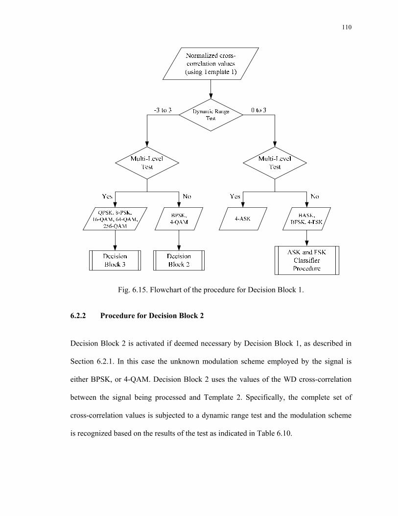
110
Fig. 6.15. Flowchart of the procedure for Decision Block 1.
6.2.2 Procedure for Decision Block 2
Decision Block 2 is activated if deemed necessary by Decision Block 1, as described in
Section 6.2.1. In this case the unknown modulation scheme employed by the signal is
either BPSK, or 4-QAM. Decision Block 2 uses the values of the WD cross-correlation
between the signal being processed and Template 2. Specifically, the complete set of
cross-correlation values is subjected to a dynamic range test and the modulation scheme
is recognized based on the results of the test as indicated in Table 6.10.

111
Table 6.10 Dynamic range of the cross-correlation data using Template 2
Dynamic Range Modulation Scheme
~0 BPSK
-3 to 3 4-QAM The procedure for Decision Block 2 is described as follows.
Step 1: The received signal is cross-correlated in the WD with Template 2 and the
values are normalized appropriately.
Step 2: A dynamic range test is applied to the resulting set of normalized cross-
correlation values and output indicators are assigned. If the data lie within the
dynamic range of -3 to 3, then the output indicator ‘0’ is assigned. If the values
are approximately equal to zero, then the output indicator ‘1’ is assigned.
Step 3: If the output indicator assigned is:
‘0,’ the modulation scheme is 4-QAM
‘1,’ the modulation scheme is BPSK.
The flowchart of the procedure is illustrated in Fig. 6.16.
Normalized cross-correlation values(using Template 2)
-3 to 3 ~0
BPSK
Dynamic RangeTest
4-QAM
Fig. 6.16. Flowchart of the procedure for Decision Block 2.

112
6.2.3 Procedure for Decision Block 3
Decision Block 3 is activated when the unknown received signal is identified by Decision
Block 1 to be in the set {QPSK, 8-PSK, 16-QAM, 64-QAM, 256-QAM}. The procedure
for Decision Block 3 is described as follows.
Step 1: The received signal is cross-correlated in the WD with Template 3 and the
values are normalized appropriately.
Step 2: A multi-level test is applied to the resulting set of normalized cross-correlation
values and output indicators are assigned. If the data are composed of single-
level values, then the output indicator ‘0’ is assigned. If the values are multi-
level, then the output indicator ‘1’ is assigned.
Step 3: If the output indicator assigned is:
‘0,’ the modulation scheme is QPSK
‘1,’ go to the PSK and QAM Classifier Procedure.
The flowchart for the above procedure is provided in Fig. 6.17.
Fig. 6.17. Flowchart of the procedure for Decision Block 3.

113
6.2.4 Procedures for Other Decision Blocks
Based on the procedures for Decision Blocks 1 and 3, there are two groups of modulation
schemes which require additional common features templates for identification. The two
groups are:
Group 1: {BASK, BFSK, 4-FSK}
Group 2: {8-PSK, 16-QAM, 64-QAM, 256-QAM}
Therefore, two additional decision making procedures need to be developed for the WD
AMR of these modulation schemes. The procedure for classifying the modulation
schemes in Group 1 is termed the ASK and FSK Classifier Procedure. While to
distinguish between the modulation schemes in Group 2, a detailed PSK and QAM
Classifier Procedure has been developed.
6.2.4.1 ASK and FSK Classifier Procedure
As mentioned in Chapter 4, and based on the definition of the FSK modulation scheme,
multiple carrier frequencies are required to represent different data symbols using FSK.
Therefore, additional common features templates are introduced in order to develop the
ASK and FSK Classifier Procedure so as to distinguish among the modulation schemes in
Group 1. Specifically, two additional common features templates, Template 4 and
Template 5, are introduced. These two new templates are illustrated in Fig. 6.18.
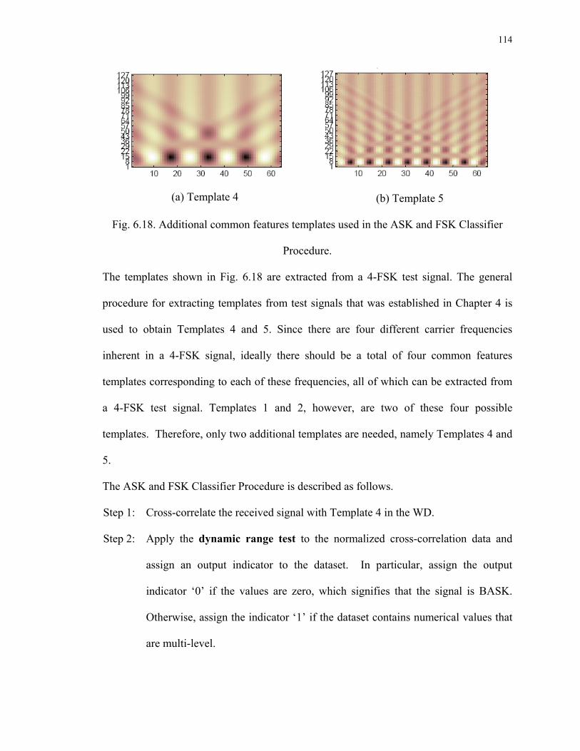
114
(a) Template 4
(b) Template 5
Fig. 6.18. Additional common features templates used in the ASK and FSK Classifier
Procedure.
The templates shown in Fig. 6.18 are extracted from a 4-FSK test signal. The general
procedure for extracting templates from test signals that was established in Chapter 4 is
used to obtain Templates 4 and 5. Since there are four different carrier frequencies
inherent in a 4-FSK signal, ideally there should be a total of four common features
templates corresponding to each of these frequencies, all of which can be extracted from
a 4-FSK test signal. Templates 1 and 2, however, are two of these four possible
templates. Therefore, only two additional templates are needed, namely Templates 4 and
5.
The ASK and FSK Classifier Procedure is described as follows.
Step 1: Cross-correlate the received signal with Template 4 in the WD.
Step 2: Apply the dynamic range test to the normalized cross-correlation data and
assign an output indicator to the dataset. In particular, assign the output
indicator ‘0’ if the values are zero, which signifies that the signal is BASK.
Otherwise, assign the indicator ‘1’ if the dataset contains numerical values that
are multi-level.
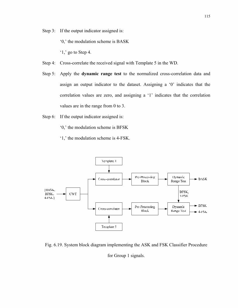
115
Step 3: If the output indicator assigned is:
‘0,’ the modulation scheme is BASK
‘1,’ go to Step 4.
Step 4: Cross-correlate the received signal with Template 5 in the WD.
Step 5: Apply the dynamic range test to the normalized cross-correlation data and
assign an output indicator to the dataset. Assigning a ‘0’ indicates that the
correlation values are zero, and assigning a ‘1’ indicates that the correlation
values are in the range from 0 to 3.
Step 6: If the output indicator assigned is:
‘0,’ the modulation scheme is BFSK
‘1,’ the modulation scheme is 4-FSK.
Fig. 6.19. System block diagram implementing the ASK and FSK Classifier Procedure
for Group 1 signals.
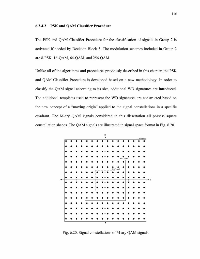
116
6.2.4.2 PSK and QAM Classifier Procedure
The PSK and QAM Classifier Procedure for the classification of signals in Group 2 is
activated if needed by Decision Block 3. The modulation schemes included in Group 2
are 8-PSK, 16-QAM, 64-QAM, and 256-QAM.
Unlike all of the algorithms and procedures previously described in this chapter, the PSK
and QAM Classifier Procedure is developed based on a new methodology. In order to
classify the QAM signal according to its size, additional WD signatures are introduced.
The additional templates used to represent the WD signatures are constructed based on
the new concept of a “moving origin” applied to the signal constellations in a specific
quadrant. The M-ary QAM signals considered in this dissertation all possess square
constellation shapes. The QAM signals are illustrated in signal space format in Fig. 6.20.
I
Q
64-QAM
16-QAM
256-QAM
Fig. 6.20. Signal constellations of M-ary QAM signals.
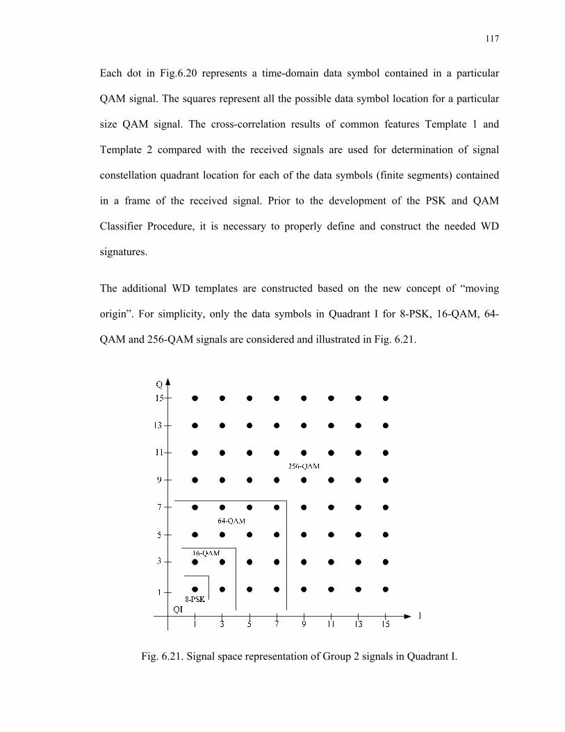
117
Each dot in Fig.6.20 represents a time-domain data symbol contained in a particular
QAM signal. The squares represent all the possible data symbol location for a particular
size QAM signal. The cross-correlation results of common features Template 1 and
Template 2 compared with the received signals are used for determination of signal
constellation quadrant location for each of the data symbols (finite segments) contained
in a frame of the received signal. Prior to the development of the PSK and QAM
Classifier Procedure, it is necessary to properly define and construct the needed WD
signatures.
The additional WD templates are constructed based on the new concept of “moving
origin”. For simplicity, only the data symbols in Quadrant I for 8-PSK, 16-QAM, 64-
QAM and 256-QAM signals are considered and illustrated in Fig. 6.21.
Fig. 6.21. Signal space representation of Group 2 signals in Quadrant I.
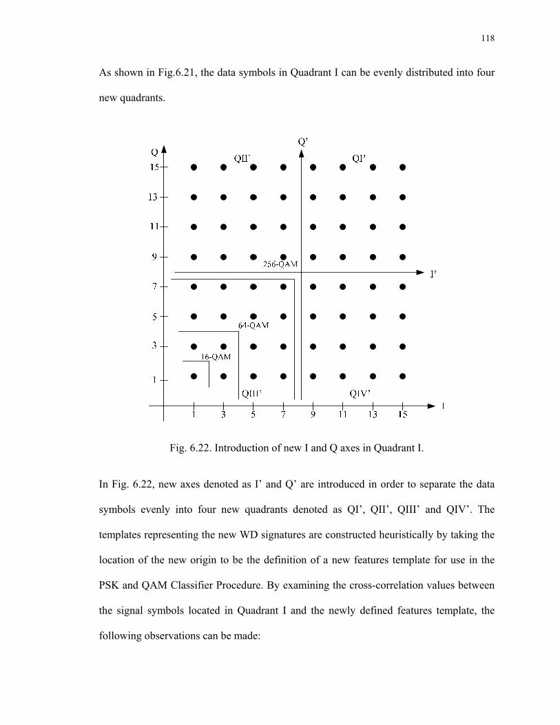
118
As shown in Fig.6.21, the data symbols in Quadrant I can be evenly distributed into four
new quadrants.
Fig. 6.22. Introduction of new I and Q axes in Quadrant I.
In Fig. 6.22, new axes denoted as I’ and Q’ are introduced in order to separate the data
symbols evenly into four new quadrants denoted as QI’, QII’, QIII’ and QIV’. The
templates representing the new WD signatures are constructed heuristically by taking the
location of the new origin to be the definition of a new features template for use in the
PSK and QAM Classifier Procedure. By examining the cross-correlation values between
the signal symbols located in Quadrant I and the newly defined features template, the
following observations can be made:
119
1. For signals representing data symbols located in the upper triangular region of
Quadrant I of the signal constellation, the cross-correlation results for the data
symbols compared to the new origin are larger than the auto-correlation value of
the features template representing the new origin.
2. On the other hand, for the signals located in the lower triangular region of
Quadrant I, the cross-correlation results for the data symbols compared to the
origin are smaller than the auto-correlation value of the new origin.
3. For the signals that are located on the diagonal co-linear with the new origin, the
cross-correlation results obtained are approximately the same as the auto-
correlation value of the new origin.
All of the above signal and template locations are illustrated graphically in Fig. 6.23. The
dashed line represented the decision boundary for upper and lower triangular region for
developing the decision rule for recognizing the different sizes of the various QAM
signals.
In Fig. 6.23, the new features template is represented as a square that is coincident with
the location of the new origin. Also in the figure, the dashed line serves as the decision
boundary reflecting the three observations made above concerning the various
comparisons between the cross-correlation and auto-correlation results. With the
introduction of this new template, and also the use of its auto-correlation value, it is now
possible to identify whether the signal is a 256-QAM signal or not. Therefore, a similar
methodology can be applied to the lower triangular region of the signal constellation in
order to classify QAM signals of smaller size.
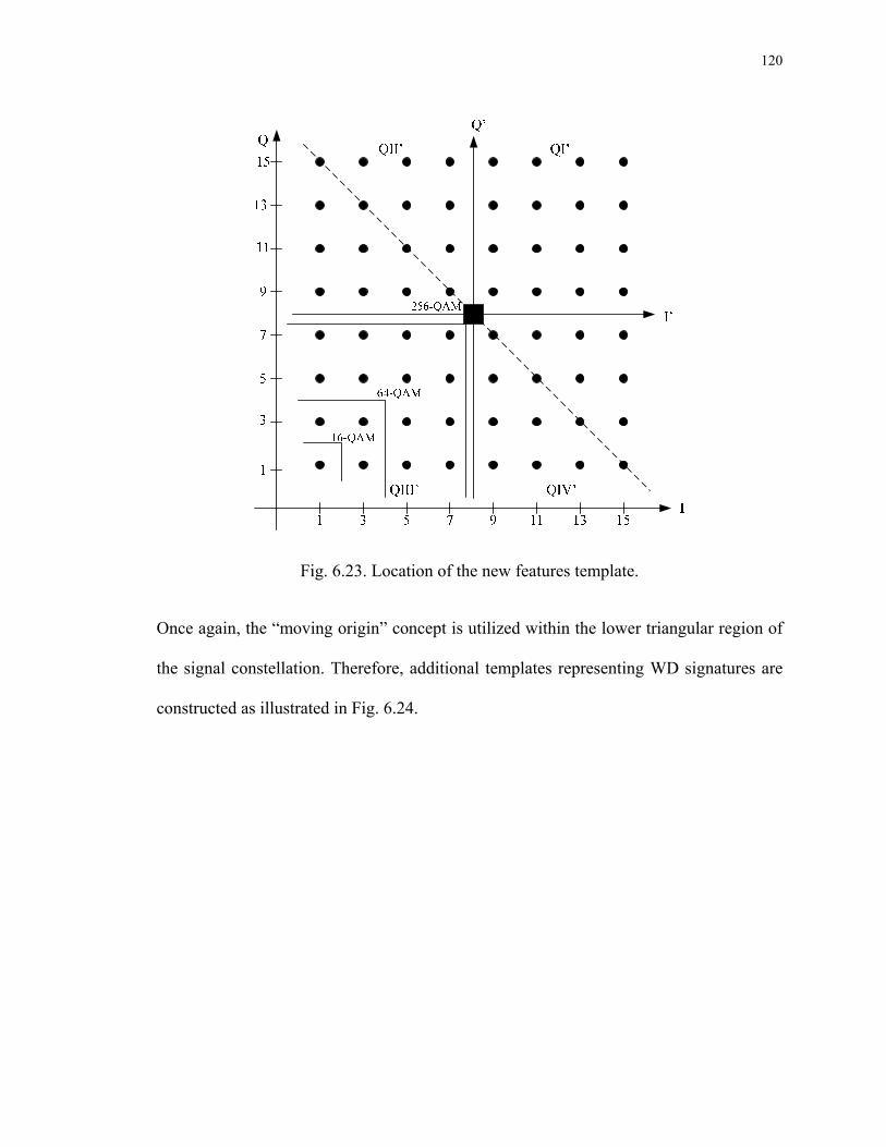
120
Fig. 6.23. Location of the new features template.
Once again, the “moving origin” concept is utilized within the lower triangular region of
the signal constellation. Therefore, additional templates representing WD signatures are
constructed as illustrated in Fig. 6.24.
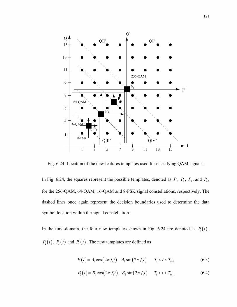
121
I
Q QI’
8-PSK
16-QAM
64-QAM
256-QAM
1 753 9 151311
1
3
5
7
9
11
13
15QII’
QIII’ QIV’
I’
Q’
P2
P1
P3
P4
Fig. 6.24. Location of the new features templates used for classifying QAM signals.
In Fig. 6.24, the squares represent the possible templates, denoted as 1P , 2P , 3P , and 4P ,
for the 256-QAM, 64-QAM, 16-QAM and 8-PSK signal constellations, respectively. The
dashed lines once again represent the decision boundaries used to determine the data
symbol location within the signal constellation.
In the time-domain, the four new templates shown in Fig. 6.24 are denoted as ( )1P t ,
( )2P t , ( )3P t and ( )4P t . The new templates are defined as
( ) ( ) ( )1 1 2 1cos 2 sin 2 c c i iP t A f t A f t T t Tπ π += − < < (6.3)
( ) ( ) ( )2 1 2 1cos 2 sin 2 c c i iP t B f t B f t T t Tπ π += − < < (6.4)

122
( ) ( ) ( )3 1 2 1cos 2 sin 2 c c i iP t C f t C f t T t Tπ π += − < < (6.5)
( ) ( ) ( )4 1 2 1cos 2 sin 2 c c i iP t D f t D f t T t Tπ π += − < < (6.6)
where 1A , 2A , 1B , 2B , 1C , 2C , 1D and 2D are constants that depend on the location of the
templates on the I and Q axes. In (6.3)-(6.6), iT represents the boundary of the ith data
symbol within a frame of the transmitted signal.
In order to distinguish a 64-QAM signal from a 256-QAM signal, not only the templates
1P , 2P and 3P are needed, but it is also required to test for special locations as shown in
Fig. 6.25. The special locations are denoted by 1S , 2S , 3S , 4S , 5S and 6S . The cross-
correlation results of the received signal with common features Template 1 and Template
2 are used for determining the special locations.
Several assumptions are made for the special locations. When the signal locations
coincide with one of the special locations in the figure, the special locations are actually
representing the signal symbols that can be present in various M-ary QAM signals. For
example, location 1S can be represented either as one of the symbols in a 256-QAM
signal, or as one of the symbols in a 64-QAM signal. Locations 2S and 3S can both be
represented as symbols in either a 64-QAM signal or a 256-QAM signal. Due to this, if
signal symbols are located at the special locations 1S , 2S or 3S , then they are categorized
as belonging to a 64-QAM signal. Symbols located at special locations 5S and 6S are
categorized as belonging to a 256-QAM signal. The same decision rules are applied to
the other three quadrants of the overall constellation.

123
P4
P3
P2
P1
I
Q
QI8-PSK
16-QAM
64-QAM
256-QAM
1 753 9 151311
1
3
5
7
9
11
13
15
S1S2
S3
S4
S5S6
Fig. 6.25. The signal space depicting the new templates with special locations indicated
in Quadrant I.
The procedure to distinguish a 64-QAM signal from a 256-QAM signal is described in
the following.
Step 1: Cross-correlate the received signal with Template 1P and compute the auto-
correlation value of 1P .
Step 2: Use the sliding cross-correlation procedure of Fig. 4.18. Compare the resulting
cross-correlation values between 1P and the received signal with the auto-
correlation value of 1P . If the cross-correlation values are larger than, or equal

124
to, the auto-correlation value, then the signal is classified as being that of a
256-QAM signal. Otherwise, cross-correlate the received signal with 2P and
compute the auto-correlation value of 2P .
Step 3: Again use the sliding operation in Fig. 4.18 to obtain cross-correlation results
for the received signal compared to Template 2P . Compare the cross-
correlation results with the auto-correlation value of 2P . If the cross-
correlation values are larger than the auto-correlation value of 2P . Test for
special location, 1S . If the cross-correlation values are approximately equal to
the auto-correlation value of 2P , test for the other special locations 2S and 3S .
Otherwise, test for the cases of special locations 4S , and 5S .
Step 4: Cross-correlate the received signal with common features Template 1 and
Template 2. If the two cross-correlation values are approximately the same,
then the signal is classified as that of a 64-QAM signal. Otherwise, the signal
is declared to be a 256-QAM signal.
Step 5: If the cross-correlation values between the received, noisy signal and Template
2P , is approximately equal to the auto-correlation value of 2P , test for the
special locations of 2S and 3S . If the cross-correlation values of Template 1
are larger than Template 2, then the signal is classified as being that of a 64-
QAM signal. Otherwise, it is declared to be a 256-QAM signal.
Step 6: If the cross-correlation values between the received signal and Template 2P is
smaller than the auto-correlation value of 2P , then test for the special locations
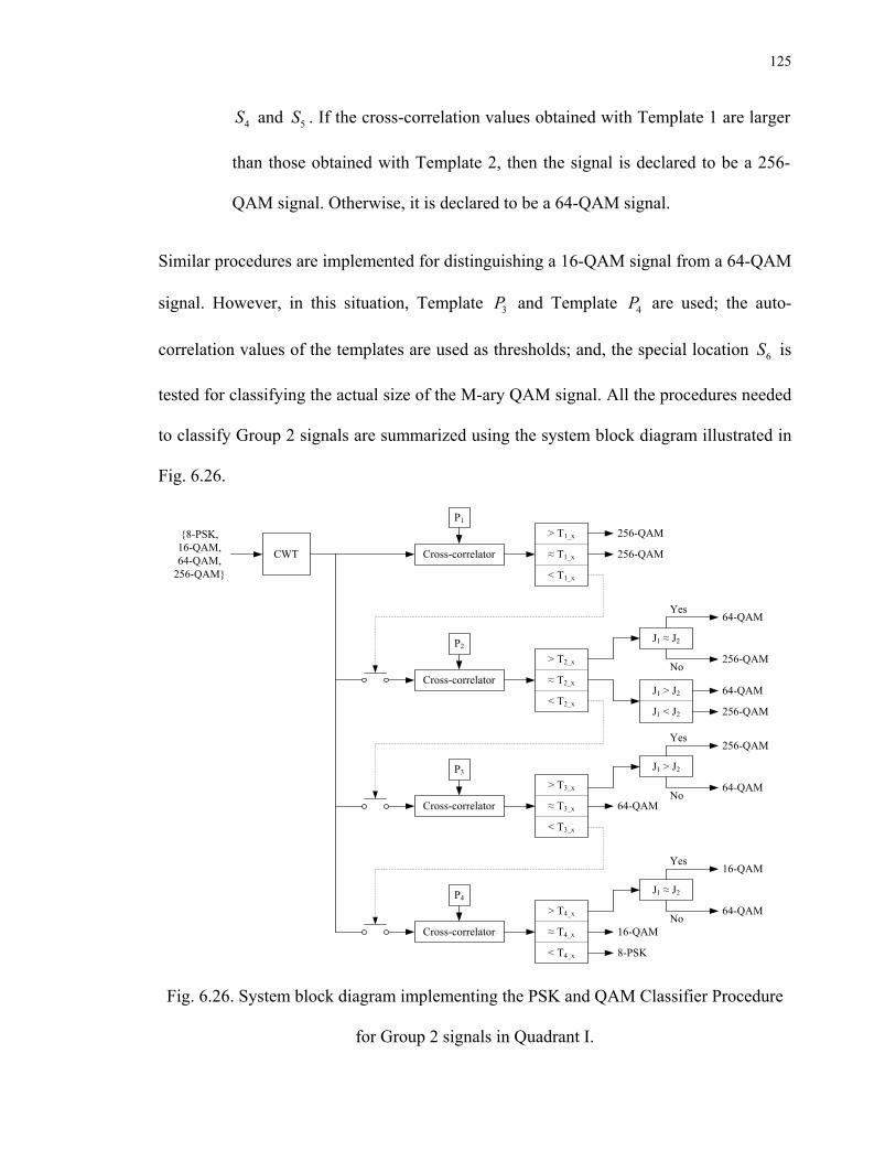
125
4S and 5S . If the cross-correlation values obtained with Template 1 are larger
than those obtained with Template 2, then the signal is declared to be a 256-
QAM signal. Otherwise, it is declared to be a 64-QAM signal.
Similar procedures are implemented for distinguishing a 16-QAM signal from a 64-QAM
signal. However, in this situation, Template 3P and Template 4P are used; the auto-
correlation values of the templates are used as thresholds; and, the special location 6S is
tested for classifying the actual size of the M-ary QAM signal. All the procedures needed
to classify Group 2 signals are summarized using the system block diagram illustrated in
Fig. 6.26.
Cross-correlator
P1
256-QAM
CWT
{8-PSK,16-QAM, 64-QAM,
256-QAM}
P2
P3
P4
> T1_x
≈ T1_x
< T1_x
> T3_x
≈ T3_x
< T3_x
> T4_x
≈ T4_x
< T4_x
256-QAM
16-QAM
8-PSK
64-QAM
J1 ≈ J2
> T2_x
≈ T2_x
< T2_x
J1 > J2
J1 < J2
64-QAM
256-QAM
64-QAM
Cross-correlator
Cross-correlator
Cross-correlator
256-QAM
Yes
No
J1 ≈ J2
16-QAM
64-QAM
Yes
No
J1 > J2
256-QAM
64-QAM
Yes
No
Fig. 6.26. System block diagram implementing the PSK and QAM Classifier Procedure
for Group 2 signals in Quadrant I.

126
The abovementioned procedure has been developed for classifying Group 2 signals in
Quadrant I. However, the same procedure is applied for signals representing data symbols
that fall into any one of the other three quadrants. The templates and also the special
locations are adjusted to the particular quadrant for classify the Group 2 signals.
The overall PSK and QAM Classifier Procedure is described as follows.
Step 1: Cross-correlate the received signal with common features Template 1 and
Template 2.
Step 2: Based on the algebraic sign of the cross-correlation result obtained in Step 1,
determine the quadrant location of the received signal.
Step 3: Cross-correlate the received signal with the quadrant specific templates.
Step 4: Follow the same procedures as described in Fig. 6.26 in order to classify the
particular signal modulation type from among those in Group 2.
6.3 Simulation Experiment and Results
The WD AMR algorithm based on the common features templates developed in Section
6.2 has been implemented in MATLAB. All of the communications test signals used in
the simulations have been corrupted by zero-mean AWGN having SNR values in the
range from -5 dB to 10 dB. The rates of correct modulation classification have been
obtained using 100,000 Monte Carlo trials. The transmitted signal used in each trial
consists of 192 symbols per frame transmitted. The signal is oversampled by a factor of
sixteen when compared to the Nyquist rate corresponding to the frequency of the
127
sinusoidal carrier. The system parameters assumed to be known for the AMR process
include the carrier frequency and perfect symbol timing with no timing offset.
The results of the experiments for all of the modulation schemes are given in Tables 6.10-
6.14, which contain the rates of correct classification for the five different SNR values,
i.e., 10 dB, 5 dB, 0 dB, -3 dB, and -5 dB.

128

129
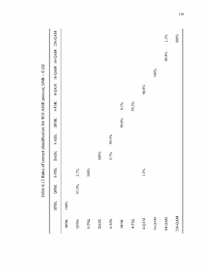
130
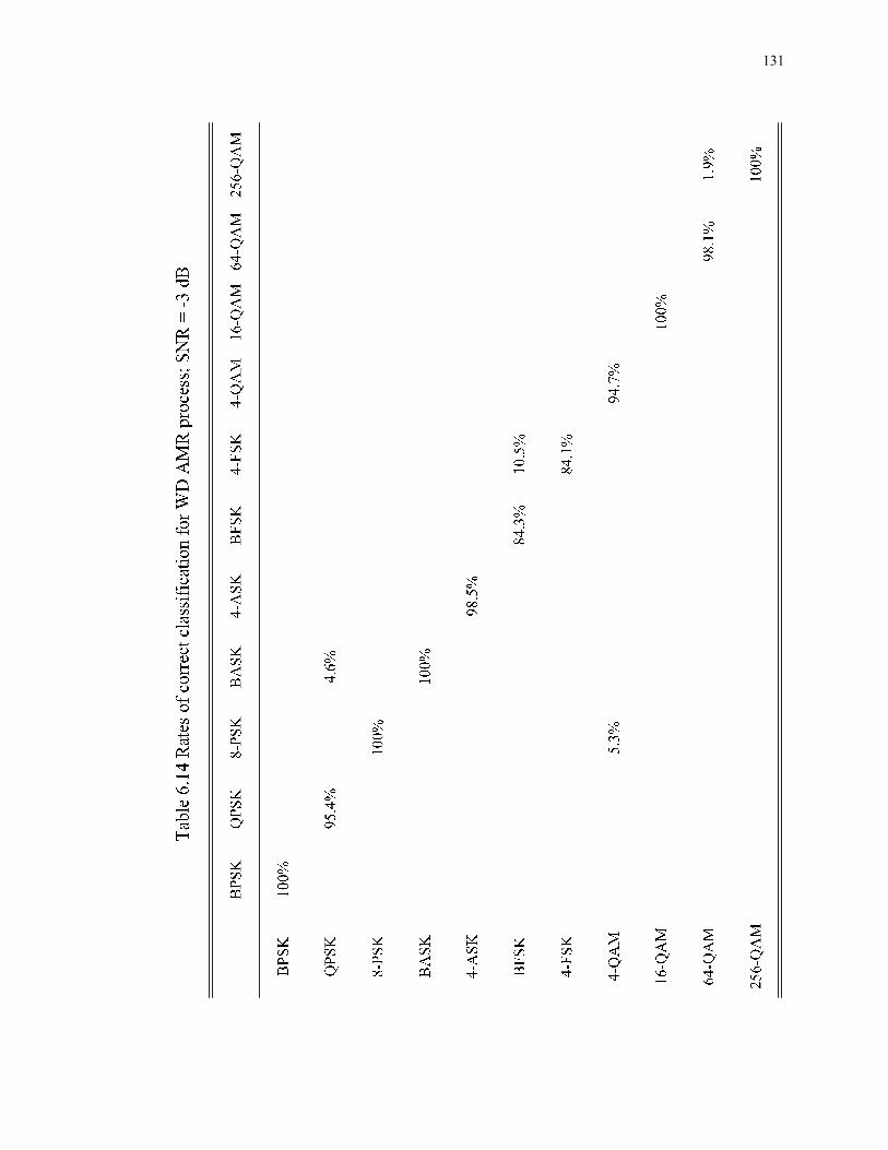
131

132

133
6.4 Comparison of Results
Several prior works on AMR that are available in the literature, which use both WT-
based and non-WT based methodologies, have been surveyed in Chapter 2. In this section
the results of simulation experiments reported in these works are compared with the
results obtained in Section 6.3. The relevant comparisons are presented in Tables 6.16-
6.18.
It must be reiterated that a direct comparison of the different AMR methodologies is
impossible due to the fact that the prior works reported in the literature do not necessarily
use the same general a priori assumptions, such as SNR values, numbers of symbols per
transmission, etc.
In this work, it must be highlighted that the actual sizes of M-ary QAM signal
constellations are identified based on a new “moving origin” concept. The majority of the
work reported in the literature focuses only on classifying signals as being ASK, FSK or
PSK. There is no work reported in which the actual sizes of the M-ary QAM signals are
classified.
From Table 6.18, the rates of correct classification at SNR = 10 dB and 5 dB, are almost
100% for all the communications signals considered in this work. In the case of SNR = 0
dB, majority of the rates of correct classification achieved are above 97%, except in the
cases of 4-FSK and 4-QAM signals for which rates of 95.3% and 96.8% were achieved,
respectively. For noisy channels operating at an SNR = -5 dB, the rates of correct
classification achieved are near, or above, 94% for most of the modulation schemes. The

134
exception at SNR = -5 dB is that of the FSK signals. The rates of correct classification at
SNR = -5 dB for BFSK and 4-FSK are 77.3% and 63.2%, respectively.
In comparison with the results reported from the literature, the rates of correct
classification obtained in this work are either equal to, or better than any other results.
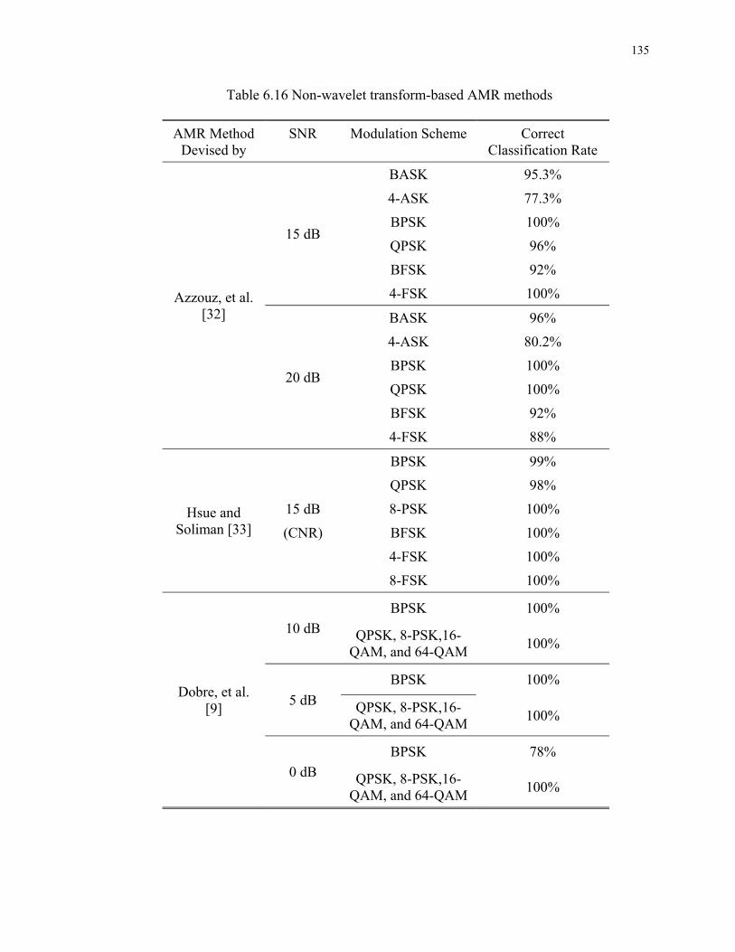
135
Table 6.16 Non-wavelet transform-based AMR methods
AMR Method Devised by
SNR Modulation Scheme Correct Classification Rate
Azzouz, et al. [32]
15 dB
BASK
4-ASK
BPSK
QPSK
BFSK
4-FSK
95.3%
77.3%
100%
96%
92%
100%
20 dB
BASK
4-ASK
BPSK
QPSK
BFSK
4-FSK
96%
80.2%
100%
100%
92%
88%
Hsue and Soliman [33]
15 dB
(CNR)
BPSK
QPSK
8-PSK
BFSK
4-FSK
8-FSK
99%
98%
100%
100%
100%
100%
Dobre, et al. [9]
10 dB BPSK 100%
QPSK, 8-PSK,16-QAM, and 64-QAM 100%
5 dB BPSK 100%
QPSK, 8-PSK,16-QAM, and 64-QAM 100%
0 dB BPSK 78%
QPSK, 8-PSK,16-QAM, and 64-QAM 100%

136
Table 6.17 Wavelet transform-based AMR methods
AMR Method Devised by
SNR Modulation Scheme Correct Classification Rate
Ho, et al. [58]
13 dB
(CNR)
BPSK
QPSK
8-PSK
2-FSK
4-FSK
8-FSK
97%
97%
97%
100%
100%
100%
Hong and Ho [60]
20 dB
(CNR)
QPSK
4-FSK
16-QAM
100%
100%
99.7%
15 dB
(CNR)
QPSK
4-FSK
16-QAM
99.5%
100%
98.7%
10 dB
(CNR)
QPSK
4-FSK
16-QAM
98.8%
100%
98.7%
5 dB
(CNR)
QPSK
4-FSK
16-QAM
97.6%
100%
100%
Jin, et al. [54]
13 dB
BPSK
QPSK
8-PSK
BFSK
4-FSK
100%
100%
100%
100%
100%
10 dB
BPSK
QPSK
8-PSK
BFSK
4-FSK
100%
99.9%
100%
98.1%
100%
8 dB
BPSK
QPSK
8-PSK
BFSK
4-FSK
100%
97.5%
100%
95.3%
100%

137
Table 6.18 AMR classification rates obtained in this research work
Modulation Scheme
SNR = 10 dB SNR = 5 dB SNR = 0 dB SNR = -5 dB
BPSK 100% 100% 100% 100%
QPSK 100% 99.8% 97.3% 94.6%
8-PSK 100% 100% 100% 100%
BASK 100% 100% 100% 95.8%
4-ASK 99.8% 99.8% 99.3% 95.9%
BFSK 100% 100% 99.9% 77.3%
4-FSK 100% 99.9% 95.3% 63.2%
4-QAM 100% 98.9% 96.8% 93.8%
16-QAM 100% 100% 100% 100%
64-QAM 100% 100% 98.1% 96.1%
256-QAM 100% 100% 100% 100%
6.5 Conclusions
In this chapter, an effective WD AMR process has been developed and its efficacy has
been demonstrated with the use of the pattern recognition technique of cross-correlation
along with templates defined in the wavelet-domain. The system parameters that are
assumed to be known for the AMR process include the carrier frequency and perfect
symbol timing with no timing offset. It has been demonstrated that the AMR process can
correctly classify signals with very high reliability even at low values of SNR. It is shown
in Tables 6.16-6.18, that the rates of correct classification obtained in this work are equal
to, or better than, those reported in the literature. Furthermore, the WD AMR algorithm
developed in this work can classify the actual sizes of M-ary QAM signal constellations
while a classification algorithm for inter-class QAM signals is absent in the literature.
138
Given the reliability of the AMR process developed in this chapter, it can be used to
advance the state of the art in communications receiver design so as to permit
interoperability between various communications standards. In other words, the AMR
process can be used to enable the development of agile radio receivers and transceivers.
Such agile radios can be used in military signal analysis applications, such as threat
analysis, spectrum management, electronic warfare, and electronics surveillance systems.
Finally, the AMR process devised can be extended to enable classification of more
modulation schemes by using similar methodologies and multiple wavelet families.
139
Chapter 7
Techniques for Demodulation Using Wavelet-Domain
Templates
Having hypothesized, described, and validated two WT-based AMR algorithms, it is now
necessary to develop the techniques for demodulation in order to complete the baseband
processing system based on the Wavelet Platform concept. After correctly classifying the
previously unknown modulation scheme employed by a received communications signal,
an appropriate demodulation process must be activated in order to recover the
information-bearing baseband data.
As described in Chapter 4, the details for constructing templates corresponding to WD
signatures for the WD AMR algorithms have been described. These two types of
templates, i.e., the unique features templates and the common features templates, are also
used to develop a WD Demodulation process. Specifically, the WD cross-correlation
results are used to obtain the decision metrics needed for the recovery of the baseband
data contained within a communications signal.
In Section 7.1, WD Demodulation techniques using the unique features templates are
developed. As with the AMR process, techniques developed using such symbol transition
templates are only suitable for binary modulated signals. WD Demodulation techniques
using the common features templates are developed in Section 7.2. The communications
signals considered in this case are BASK, 4-ASK, BFSK, 4-FSK, BPSK, QPSK, 8-PSK,
4-QAM (also denoted as 4π -QPSK), 16-QAM, 64-QAM and 256-QAM. In addition, a
140
new methodology is developed in this chapter for the demodulation of M-ary QAM
signals. The performance of the demodulation techniques is evaluated and BER curves
are plotted for cases of signals corrupted with AWGN resulting in SNR values in the
range from -5 dB to 10 dB.
7.1 Demodulation Using Unique Features Templates
The WD Demodulation techniques for digitally modulated communications signals are
developed based on the cross-correlation of the received communications signals with the
unique features templates in the WD. The cross-correlation data are then compared with
the auto-correlation values for each of the unique features templates. The result of the
comparison is assigned an indicator. Based on the indicator the data bit sequence can then
be recovered. Fig. 7.1 illustrates the system block diagram for the demodulation
procedures for BASK, BFSK or BPSK signals using the unique features templates. The
functionality of the pre-processing block is to normalize the cross-correlation values to
have a dynamic range from -3 to 3.
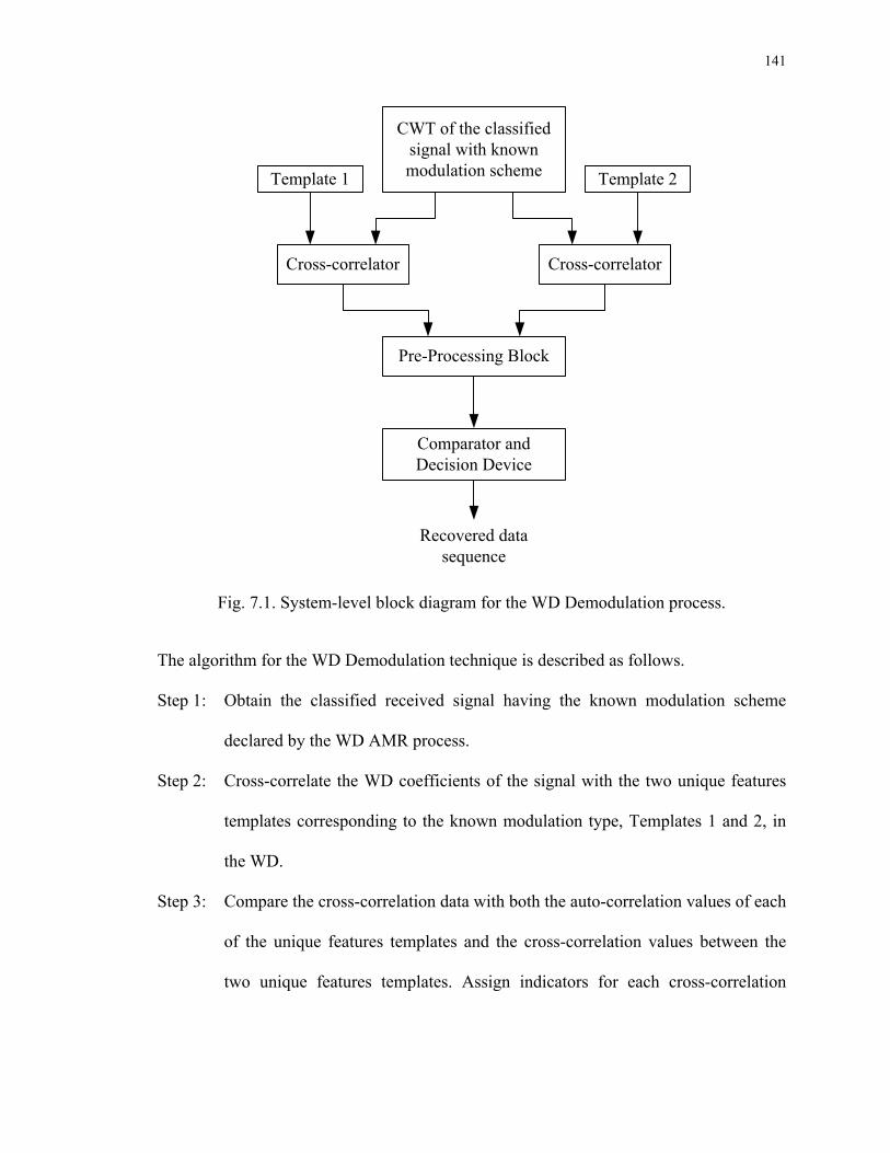
141
CWT of the classified signal with known modulation scheme
Cross-correlator Cross-correlator
Template 1 Template 2
Comparator and Decision Device
Recovered data sequence
Pre-Processing Block
Fig. 7.1. System-level block diagram for the WD Demodulation process.
The algorithm for the WD Demodulation technique is described as follows.
Step 1: Obtain the classified received signal having the known modulation scheme
declared by the WD AMR process.
Step 2: Cross-correlate the WD coefficients of the signal with the two unique features
templates corresponding to the known modulation type, Templates 1 and 2, in
the WD.
Step 3: Compare the cross-correlation data with both the auto-correlation values of each
of the unique features templates and the cross-correlation values between the
two unique features templates. Assign indicators for each cross-correlation

142
value obtained at each signal segment corresponding to a data symbol period.
Step 4: Based on the results from Step 3, output the data bit sequence.
Fig. 7.2. Example of WD Demodulation process using Templates 1 and 2.
An example of the demodulation process using the unique features templates for a signal
with a known modulation scheme is illustrated in Fig. 7.2. The demodulation process is
based on the cross-correlation between the WD scalogram of the known signal having a
modulation signal and the WD scalogram of the appropriate features templates. For
clarity, the unknown transmitted data are illustrated in the top row of the figure. First, the
transformed signal with known modulation type is cross-correlated at each symbol
transition with the two unique features templates in the WD corresponding to the
modulation type. Two sets of cross-correlation results are obtained. Each resulting data
element in the cross-correlation dataset represents the cross-correlation value between
specific transition location of the communications signal at a specific transition location
and the unique features template. In Fig. 7.2, the following notations are used:
H High cross-correlation value
L Low cross-correlation value

143
M Intermediate cross-correlation value within the cross-correlation dataset
Next, each of cross-correlation values is compared with two threshold values. One
threshold value corresponds to the cross-correlation between two distinct unique features
templates, yP . The other threshold value corresponds to the auto-correlation of one of the
unique features templates, xP . The auto-correlation values are the same for both
templates because the templates are mirror images of each other. Therefore, only one of
the auto-correlation values is used as the threshold value. With the use of the two
threshold values applied to the cross-correlation dataset, the decision rule is defined as
followings
' ' output ' '
' '
x
y x
y
H x PM P x PL x P
⎧ ≥⎪= < <⎨⎪ ≤⎩
(7.1)
where x is a cross-correlation value obtained when comparing the communications signal
with a unique features template at each symbol transition location, as shown in Fig. 7.2.
Here again, xP is the auto-correlation value of the template, and yP is the value of cross-
correlation between Template 1 and Template 2. The notation H indicates that the cross-
correlation value is larger than xP , while M denotes that the value of the cross-correlation
is in between xP and yP , and L indicates that the value is less than Py.
The cross-correlation operation is computed for every symbol transition in a binary
modulation communications signal. Based on (7.1), a decision algorithm can be
developed to recover the digital data sent by the transmitter.

144
This algorithm has been implemented in MATLAB. Using Monte Carlo simulations the
BER performances have been obtained for the binary digitally modulated test signals, i.e.,
BASK, BFSK, and BPSK. Typically, the BER is very low, with only a few errors
occurring at SNR = -5 dB. The results at different SNR values are presented in Table 7.1.
Table 7.1 BER results for WD Demodulation process using unique features templates
Modulation Scheme SNR BER
BPSK
-5 dB
0 dB
5 dB
0.001
0
0
BASK
-5 dB
0 dB
5 dB
0.023
0.001
0
BFSK
-5 dB
0 dB
5 dB
10 dB
0.049
0.037
0.001
0
As seen from the results, the WD Demodulation process is very successful. There is,
however, a drawback to this demodulation process when used for binary modulated
signals. The digital data cannot be recovered if the data bit sequence is made up entirely
of either all data “1”s or all data “0”s. This is due to the use of unique features templates.
The unique features templates are defined based on symbol transitions within a
communications signals as described in Section 4.1. When there are no symbol
transitions within a communications signals, the decision algorithm will not be able to
detect symbol transitions since they are not present. The resulting BER would, therefore,
either be 100% or 0% as the system would pick the symbols to be either ‘1’ or ‘0’ by
145
default. In order to overcome this deficiency, a Return-to-Zero (RZ) data symbol format
is required instead of the Non-Return-to-Zero (NRZ) data symbol format that was used in
this work. In the next section, a WD Demodulation process based on the use of the
common features templates is explored.
7.2 Demodulation Using Common Features Templates
A WD demodulation process that utilizes the common features templates instead of the
unique features templates is now developed in this section. Again, the templates are
cross-correlated with the communications signal in the WD. The normalized cross-
correlation values are used to develop a new decision metric that is needed to recover the
baseband data sequence. The common features templates defined in Section 4.1 are
utilized for the demodulation of M-ary PSK signals. The demodulation of PSK signals is
described in Section 7.2.1. Additional common features templates are, however, required
to demodulate M-ary FSK, M-ary ASK and M-ary QAM signals. These additional
templates will be described Sections 7.2.2-7.2.4.
7.2.1 Demodulation Techniques for Phase Shift Keyed Signals
In order to demodulate M-ary PSK signals, the common features templates defined in
Section 6.1 are used. The first step of the demodulation process is to cross-correlate the
received communications signal with the appropriate common features templates in the
WD. Based on the cross-correlation results, several decision metrics are developed in
order to recover the baseband data. The common features templates used here are denoted
as Template 1, Template 2 and Template 3, all of which are illustrated in Fig. 6.2.
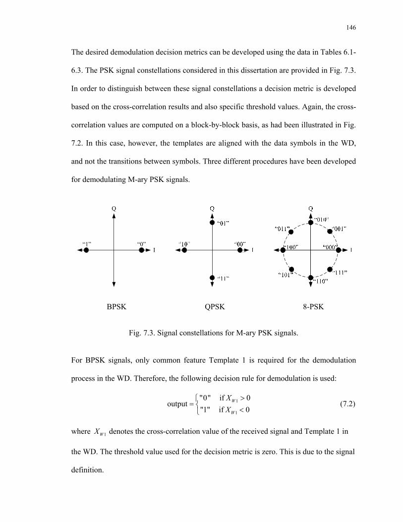
146
The desired demodulation decision metrics can be developed using the data in Tables 6.1-
6.3. The PSK signal constellations considered in this dissertation are provided in Fig. 7.3.
In order to distinguish between these signal constellations a decision metric is developed
based on the cross-correlation results and also specific threshold values. Again, the cross-
correlation values are computed on a block-by-block basis, as had been illustrated in Fig.
7.2. In this case, however, the templates are aligned with the data symbols in the WD,
and not the transitions between symbols. Three different procedures have been developed
for demodulating M-ary PSK signals.
I
Q
“0”“1”
BPSK
QPSK
8-PSK
Fig. 7.3. Signal constellations for M-ary PSK signals.
For BPSK signals, only common feature Template 1 is required for the demodulation
process in the WD. Therefore, the following decision rule for demodulation is used:
1
1
"0" if 0output
"1" if 0W
W
XX
>⎧= ⎨ <⎩
(7.2)
where 1WX denotes the cross-correlation value of the received signal and Template 1 in
the WD. The threshold value used for the decision metric is zero. This is due to the signal
definition.

147
The algorithm for the demodulation of BPSK signals in the WD using the decision metric
in (7.2) is described as follows.
Step 1: Cross-correlate the received BPSK signal with Template 1 in the WD.
Step 2: Compare each of the cross-correlation values with the fixed threshold, and
assign an indicator for each cross-correlation value.
Step 3: Based on the indicator, output the baseband data.
The algorithm described above is illustrated in Fig. 7.4.
><
1WX
Fig. 7.4. System block diagram for the BPSK demodulator in the WD.
Based on the signal constellation for the QPSK modulation scheme, it is necessary to use
both common features Template 1 and Template 2. The decision rule is described as
1 2
1 2
1 2
1 2
"00" if 0 and ~ 0 "01" if ~ 0 and 0
output = "10" if 0 and ~ 0 "11" if ~ 0 and 0
W W
W W
W W
W W
X XX XX XX X
> =⎧⎪ = >⎪⎨ < =⎪⎪ = <⎩
(7.3)
where 1WX is the value resulting from the cross-correlation of the signal with Template 1,
and 2WX is the value resulting from the cross-correlation of the signal with Template 2 in
the WD.

148
Based on (7.3), the algorithm for demodulating QPSK signals in the WD is described as
follows.
Step 1: Cross-correlate the received QPSK signal with Templates 1 and 2 in the WD.
Step 2: Examine each segment of the cross-correlation data for both Template 1 and
Template 2 and assign indicators for each segment. Apply the decision rule in
Eqn. (7.3) to the correlation values and assign an indicator for each cross-
correlation value.
Step 3: Based on the indicator, output the baseband data.
The QPSK demodulation algorithm described above is illustrated in Fig. 7.5.
“00”
“01”Cross-correlator
Template 1
WD QPSK Signal
Cross-correlator
Template 2
1 0WX >2 ~ 0WX =
1 ~ 0WX =2 0WX <
1 0WX <2 ~ 0WX =
2 0WX >1 ~ 0WX =
“10”
“11”
1WX
2WX
Fig. 7.5. System block diagram for the QPSK demodulator in the WD.
Having defined the demodulation techniques for BPSK and QPSK, a demodulation
technique for 8-PSK is now described. In this case all three common features templates
and the observations from Tables 6.1-6.3 are used for development of the decision rule.
The decision rule is described according to

149
1 2 3
1 2 3
1 2 3
1 2 3
1 2
"000" if 0, ~ 0 and 0"001" if 0, 0 and 0"010" if ~ 0, 0 and 0"011" if 0, 0 and ~ 0
output"100" if 0, ~
W W W
W W W
W W W
W W W
W W
X X XX X XX X XX X XX X
> = <> > <= > <
< > ==
< 3
1 2 3
1 2 3
1 2 3
0 and 0"101" if 0, 0 and 0"110" if ~ 0, 0 and 0"111" if 0, 0 and ~ 0
W
W W W
W W W
W W W
XX X XX X XX X X
⎧⎪⎪⎪⎪⎪⎨ = >⎪⎪ < < >⎪
= < >⎪⎪ > < =⎩
(7.4)
where 1WX , 2WX and 3WX are the cross-correlation values that result from comparing
the received signal with Template 1, Template 2 and Template 3, respectively.
Based on (7.4), the algorithm for demodulating an 8-PSK signal is described as follows.
Step 1: Cross-correlate the received 8-PSK signal with Templates 1, 2 and 3 in the WD.
Step 2: Compare the resulting cross-correlation data with the threshold value of zero as
described in Eqn. (7.4).
Step 3: Based on the result from Step 2, assign an appropriate indicator corresponding
to one of the threshold combinations shown in Eqn. (7.4).
Step 4: Based on the indicator, output the baseband data.
The 8-PSK demodulation algorithm is described above is shown in Fig. 7.6.

150
“000”
“001”Cross-correlator
Template 1
WD 8-PSK Signal
Cross-correlator
Template 2
“010”
“011”
Cross-correlator
Template 3
1 0WX >2 ~ 0WX =
3 0WX <
1 0WX >2 0WX >3 0WX <
1 ~ 0WX =2 0WX >3 0WX <
1 0WX <
3 ~ 0WX =
1 0WX <2 ~ 0WX =
3 0WX >
1 0WX <2 0WX <3 0WX >
2 0WX >
1 ~ 0WX =2 0WX <3 0WX >
1 0WX >2 0WX <
3 ~ 0WX =
“100”
“101”
“110”
“111”
1WX
2WX
3WX
Fig. 7.6. System block diagram for the 8-PSK demodulator in the WD.
7.2.2 Demodulation Techniques for Frequency Shift Keyed Signals
Recall from Chapter 6 that in order to perform a WD AMR process for M-ary FSK
signals, it was required to introduce additional common features templates along with
Template 1 and Template 2. Similarly, in the WD Demodulation process, additional
templates are required. The same templates described in Section 6.2.3.1 are used here.
Therefore, the common features templates used are Templates 1, 4 and 5.
In order to demodulate BFSK signals, only Template 1 is used. The demodulation
decision rule is described as follows
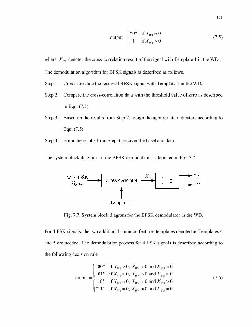
151
1
1
"0" if 0output
"1" if 0W
W
XX
≈⎧= ⎨ >⎩
(7.5)
where 1WX denotes the cross-correlation result of the signal with Template 1 in the WD.
The demodulation algorithm for BFSK signals is described as follows.
Step 1: Cross-correlate the received BFSK signal with Template 1 in the WD.
Step 2: Compare the cross-correlation data with the threshold value of zero as described
in Eqn. (7.5).
Step 3: Based on the results from Step 2, assign the appropriate indicators according to
Eqn. (7.5)
Step 4: From the results from Step 3, recover the baseband data.
The system block diagram for the BFSK demodulator is depicted in Fig. 7.7.
~=>
1WX
Fig. 7.7. System block diagram for the BFSK demodulator in the WD.
For 4-FSK signals, the two additional common features templates denoted as Templates 4
and 5 are needed. The demodulation process for 4-FSK signals is described according to
the following decision rule
1 4 5
1 4 5
1 4 5
1 4 5
"00" if 0, 0 and 0"01" if 0, 0 and 0
output"10" if 0, 0 and 0"11" if 0, 0 and 0
W W W
W W W
W W W
W W W
X X XX X XX X XX X X
> ≈ ≈⎧⎪ ≈ > ≈⎪= ⎨ ≈ ≈ >⎪⎪ ≈ ≈ ≈⎩
(7.6)
152
where 1WX , 4WX and 5WX are the cross-correlation values obtained when comparing the
received, noisy signal to Templates 1, 4 and 5, respectively.
Based on (7.6), the algorithm for demodulating 4-FSK signals in the WD is described as
follows.
Step 1: Cross-correlate the received 4-FSK signal with Templates 1, 4 and 5 in the WD.
Step 2: Compare the cross-correlation data with the threshold value of zero as described
in Eqn. (7.6).
Step 3: Based on the results from Step 2, assign appropriate indicators corresponding to
one of the threshold combinations.
Step 4: From the results of Step 3, recover the baseband data.
The corresponding block diagram for the demodulation of 4-FSK is illustrated in Fig. 7.8.
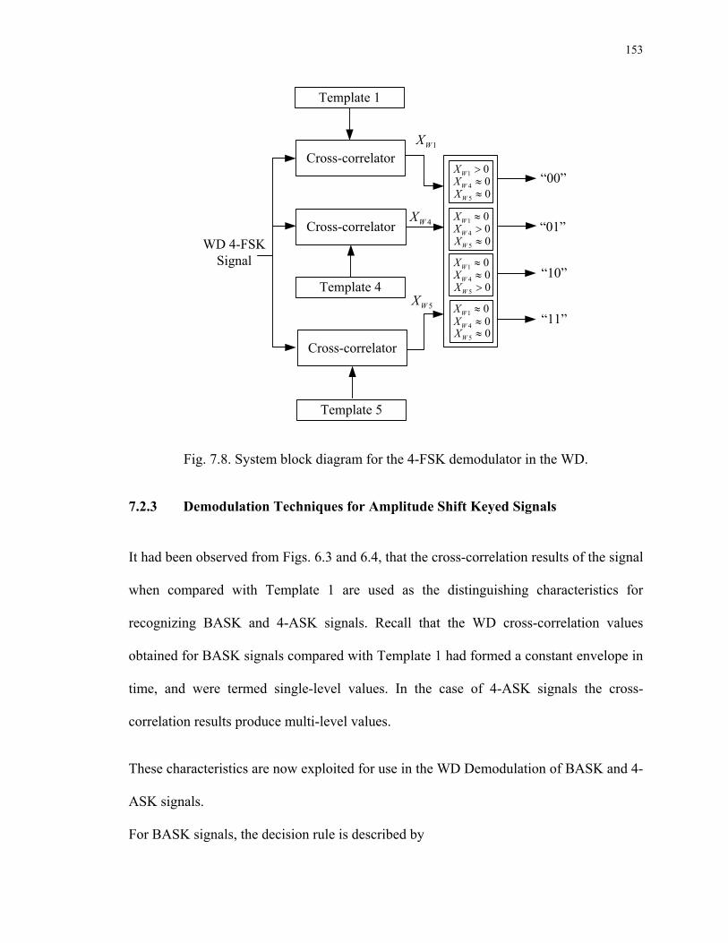
153
“00”
“01”
Cross-correlator
Template 1
WD 4-FSK Signal
Cross-correlator
Template 4“10”
“11”
Cross-correlator
Template 5
1 0WX >4 0WX ≈5 0WX ≈
1 0WX ≈4 0WX >5 0WX ≈
1 0WX ≈4 0WX ≈5 0WX >
1 0WX ≈
5 0WX ≈4 0WX ≈
1WX
4WX
5WX
Fig. 7.8. System block diagram for the 4-FSK demodulator in the WD.
7.2.3 Demodulation Techniques for Amplitude Shift Keyed Signals
It had been observed from Figs. 6.3 and 6.4, that the cross-correlation results of the signal
when compared with Template 1 are used as the distinguishing characteristics for
recognizing BASK and 4-ASK signals. Recall that the WD cross-correlation values
obtained for BASK signals compared with Template 1 had formed a constant envelope in
time, and were termed single-level values. In the case of 4-ASK signals the cross-
correlation results produce multi-level values.
These characteristics are now exploited for use in the WD Demodulation of BASK and 4-
ASK signals.
For BASK signals, the decision rule is described by
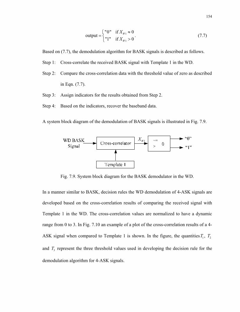
154
1
1
"0" if 0output
"1" if 0W
W
XX
≈⎧= ⎨ >⎩
. (7.7)
Based on (7.7), the demodulation algorithm for BASK signals is described as follows.
Step 1: Cross-correlate the received BASK signal with Template 1 in the WD.
Step 2: Compare the cross-correlation data with the threshold value of zero as described
in Eqn. (7.7).
Step 3: Assign indicators for the results obtained from Step 2.
Step 4: Based on the indicators, recover the baseband data.
A system block diagram of the demodulation of BASK signals is illustrated in Fig. 7.9.
~=>
1WX
Fig. 7.9. System block diagram for the BASK demodulator in the WD.
In a manner similar to BASK, decision rules the WD demodulation of 4-ASK signals are
developed based on the cross-correlation results of comparing the received signal with
Template 1 in the WD. The cross-correlation values are normalized to have a dynamic
range from 0 to 3. In Fig. 7.10 an example of a plot of the cross-correlation results of a 4-
ASK signal when compared to Template 1 is shown. In the figure, the quantities 1T , 2T
and 3T represent the three threshold values used in developing the decision rule for the
demodulation algorithm for 4-ASK signals.
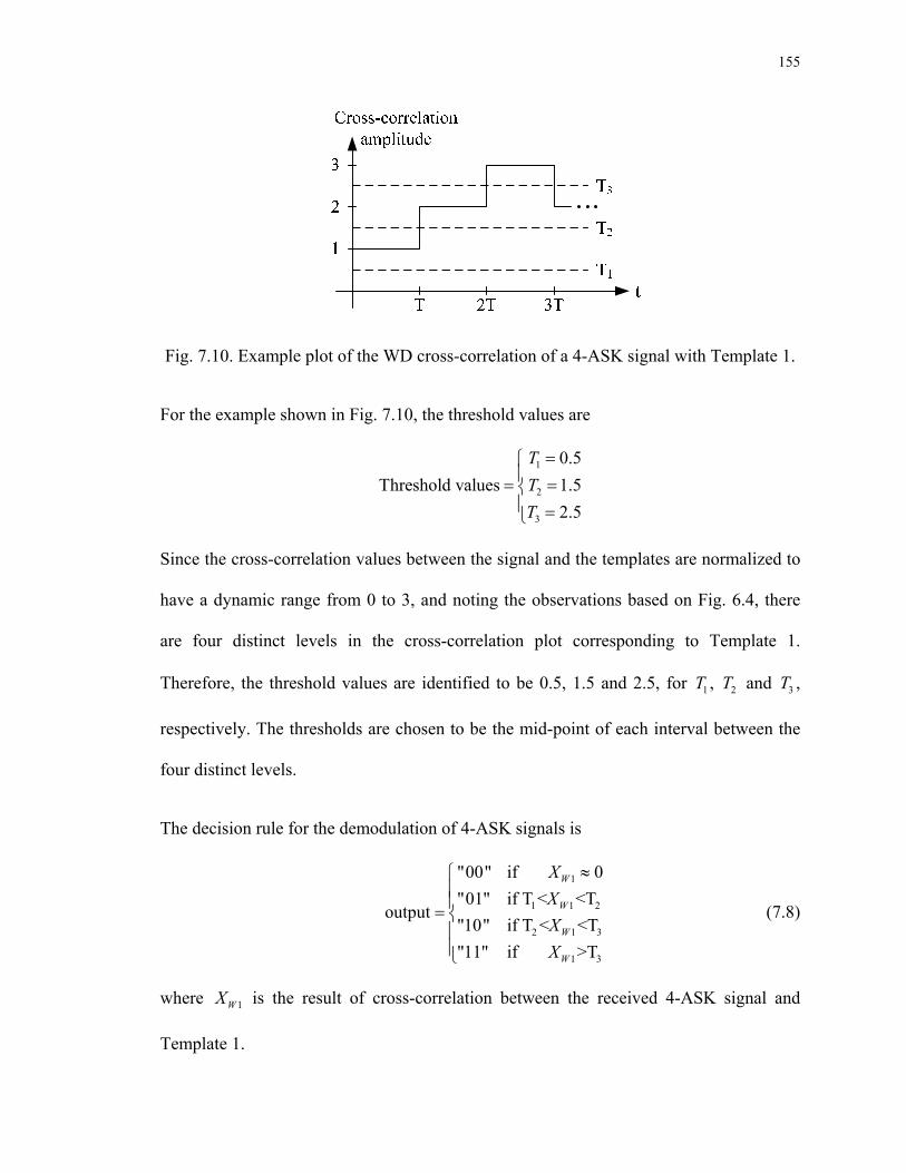
155
Fig. 7.10. Example plot of the WD cross-correlation of a 4-ASK signal with Template 1.
For the example shown in Fig. 7.10, the threshold values are
1
2
3
0.5Threshold values 1.5
2.5
TTT
=⎧⎪= =⎨⎪ =⎩
Since the cross-correlation values between the signal and the templates are normalized to
have a dynamic range from 0 to 3, and noting the observations based on Fig. 6.4, there
are four distinct levels in the cross-correlation plot corresponding to Template 1.
Therefore, the threshold values are identified to be 0.5, 1.5 and 2.5, for 1T , 2T and 3T ,
respectively. The thresholds are chosen to be the mid-point of each interval between the
four distinct levels.
The decision rule for the demodulation of 4-ASK signals is
1
1 1 2
2 1 3
1 3
"00" if 0"01" if T < <T
output"10" if T < <T"11" if >T
W
W
W
W
XXXX
≈⎧⎪⎪= ⎨⎪⎪⎩
(7.8)
where 1WX is the result of cross-correlation between the received 4-ASK signal and
Template 1.

156
The demodulation algorithm for 4-ASK is described as follows.
Step 1: Cross-correlate the received 4-ASK signal with Template 1 in the WD.
Step 2: Compare the cross-correlation data with the threshold values 1T , 2T , and 3T ,
according to Eqn. (7.8).
Step 3: Based on the results from Step 2, assign indicators for each cross-correlation
data element.
Step 4: Recover the baseband data based on the indicators assigned in Step 3.
A system block diagram describing the demodulation algorithm for 4-ASK signals is
depicted in Fig. 7.11.
1 0WX ≈
1 3WX T>
1 1 2WT X T< <
2 1 3WT X T< <
1WX
Fig.7.11. System block diagram for the 4-ASK demodulator in the WD.
7.2.4 Demodulation Techniques for Quadrature Amplitude Modulated Signals
QAM signals consist of amplitude and phase changes made to a carrier wave in order to
represent different baseband data symbols. The demodulation methodologies developed
here are again based on the cross-correlation values obtained when comparing M-ary

157
QAM signals with common features templates in the WD. The threshold values are
defined as the auto-correlation values of the templates as described in Section 6.2.3.2.
Also, additional templates are required for demodulation of the M-ary QAM signals. This
is due to the requirement that the different sizes of signal constellations be identified for
various M-ary QAM signals. The methods of extracting these templates are similar to the
methods used in the WD AMR process for M-ary QAM signals. The concept of a
“moving origin” is also used in constructing the templates representing the WD
signatures for the M-ary QAM signals. Figs. 7.12-14 illustrate the locations of the
additional common features templates for different size M-ary QAM signal
constellations. With the use of common features Template 1, Template 2 and the
additional templates, the baseband data represented by M-ary QAM symbols can be
recovered throughout an entire frame.
P7
I
Q
1 3
1
3
Fig. 7.12. Quadrant I of the 16-QAM signal constellation.

158
Fig. 7.13. Quadrant I of the 64-QAM signal constellation.
P1
P4
P5
P6
P7
P2
P3
I
Q
1 3 5 7 9 11 13 15
1
3
5
7
9
11
13
15
Fig. 7.14. Quadrant I of the 256-QAM signal constellation.
159
Again, only the first quadrant of the signal constellations for the 16-, 64- and 256-QAM
schemes are shown in Figs. 7.12-7.14, along with locations of the additional templates
required, namely 1P , 2P , …, 7P . The same concepts, however, can readily be applied to
the other 3 quadrants. The additional common features represented by the template in
Figs. 7.12-7.14 are defined in the time-domain as
( ) ( ) ( )1 1 2cos 2 sin 2c cP t A f t A f tπ π= + 1i iT t T +< < (7.9)
( ) ( ) ( )2 1 2cos 2 sin 2c cP t B f t B f tπ π= + 1i iT t T +< < (7.10)
( ) ( ) ( )3 1 2cos 2 sin 2c cP t C f t C f tπ π= + 1i iT t T +< < (7.11)
( ) ( ) ( )4 1 2cos 2 sin 2c cP t D f t D f tπ π= + 1i iT t T +< < (7.12)
( ) ( ) ( )5 1 2cos 2 sin 2c cP t E f t E f tπ π= + 1i iT t T +< < (7.13)
( ) ( ) ( )6 1 2cos 2 sin 2c cP t F f t F f tπ π= + 1i iT t T +< < (7.14)
( ) ( ) ( )7 1 2cos 2 sin 2c cP t G f t G f tπ π= + 1i iT t T +< < . (7.15)
where Aj, Bj, Cj, Dj, Ej, Fj and Gj, for j = 1, 2, are constants. The appropriate values for the
constants are assigned depending on the particular size of the signal constellation.
Appendix C lists the values of the constants used for the common features templates for
M-ary QAM signals.
The methodology for demodulating 4-QAM signals is similar to the demodulation of
QPSK signals. However, for 4-QAM signals the cross-correlation results are obtained
with Templates 1 and 3 instead of Templates 1 and 2 as was done in the case of QPSK
signals. Again, using observations based on Table 6.3 and Fig. 6.10, the decision rule for
the 4-QAM modulation scheme is

160
1 3
1 3
1 3
1 3
"00" if 0 and 0"01" if 0 and 0
output"10" if 0 and 0"11" if 0 and 0
W W
W W
W W
W W
X XX XX XX X
> <⎧⎪ < ≈⎪= ⎨ < >⎪⎪ > ≈⎩
(7.16)
where 1WX denotes the cross-correlation values obtained by comparing the received 4-
QAM signal with Template 1, and 3WX represents the cross-correlation values obtained
with Template 3.
The algorithm for demodulation of 4-QAM signals is described as follows.
Step 1: Cross-correlate the received 4-QAM signal with Template 1 and Template 3 in
the WD.
Step 2: Compare the cross-correlation data with the threshold value of zero.
Step 3: Based on the results from Step 2, assign an indicator to each individual
comparison using Eqn. (7.16).
Step 4: Recover the baseband data sequence based the indicators assigned in Step 3.
A system block diagram for the demodulation of 4-QAM signals is illustrated in Fig.
7.15.
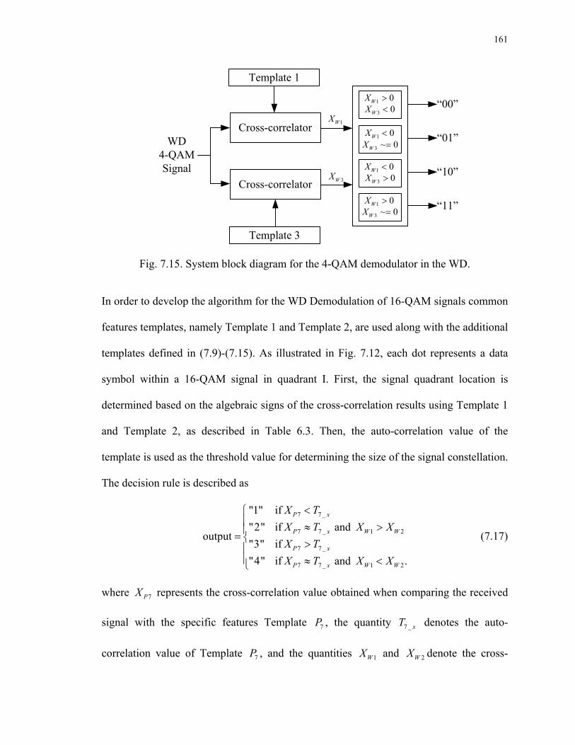
161
“00”
“01”Cross-correlator
Template 1
WD 4-QAM Signal
Cross-correlator
Template 3
1 0WX >3 0WX <
1 0WX >3 ~ 0WX =
1 0WX <3 0WX >
3 ~ 0WX =1 0WX <
“10”
“11”
1WX
3WX
Fig. 7.15. System block diagram for the 4-QAM demodulator in the WD.
In order to develop the algorithm for the WD Demodulation of 16-QAM signals common
features templates, namely Template 1 and Template 2, are used along with the additional
templates defined in (7.9)-(7.15). As illustrated in Fig. 7.12, each dot represents a data
symbol within a 16-QAM signal in quadrant I. First, the signal quadrant location is
determined based on the algebraic signs of the cross-correlation results using Template 1
and Template 2, as described in Table 6.3. Then, the auto-correlation value of the
template is used as the threshold value for determining the size of the signal constellation.
The decision rule is described as
7 7 _
7 7 _ 1 2
7 7 _
7 7 _ 1 2
"1" if "2" if and
output"3" if "4" if and .
P x
P x W W
P x
P x W W
X TX T X XX TX T X X
<⎧⎪ ≈ >⎪= ⎨ >⎪⎪ ≈ <⎩
(7.17)
where 7PX represents the cross-correlation value obtained when comparing the received
signal with the specific features Template 7P , the quantity 7 _ xT denotes the auto-
correlation value of Template 7P , and the quantities 1WX and 2WX denote the cross-

162
correlation value obtained with common features Template 1 and Template 2,
respectively.
Based on (7.17) and Table 6.3, the algorithm for the demodulation of 16-QAM signals in
the WD is described as follows.
Step 1: Cross-correlate the received 16-QAM signal with Templates 1 and 2 in the WD.
Step 2: Determine the quadrant location of each data symbol and cross-correlate
Template 7P with the signal.
Step 3: Compute the auto-correlation of 7P .
Step 4: Compare the cross-correlation results from Step 1 with the thresholds as
described in Eqn. (7.17), and assign the appropriate indicator for each signal
segment.
Step 5: Recover the baseband data sequence based on the results obtained in Step 4.
A similar methodology is applied to both 64- and 256-QAM with additional templates
introduced. The detailed algorithms and decision rules are described in Appendices A and
B.
7.3 Simulation Experiments and Results
The algorithms developed in this chapter are all realized using the MATLAB computer
simulation environment. All of the signals used in this study have been corrupted by
zero-mean AGWN resulting in SNR values in the range of -5 dB to 10 dB. The WD
Demodulator performance has been evaluated based on 105 Monte Carlos trials wherein
each simulation experiment consists of 192 bits per frame for ASK, FSK and PSK
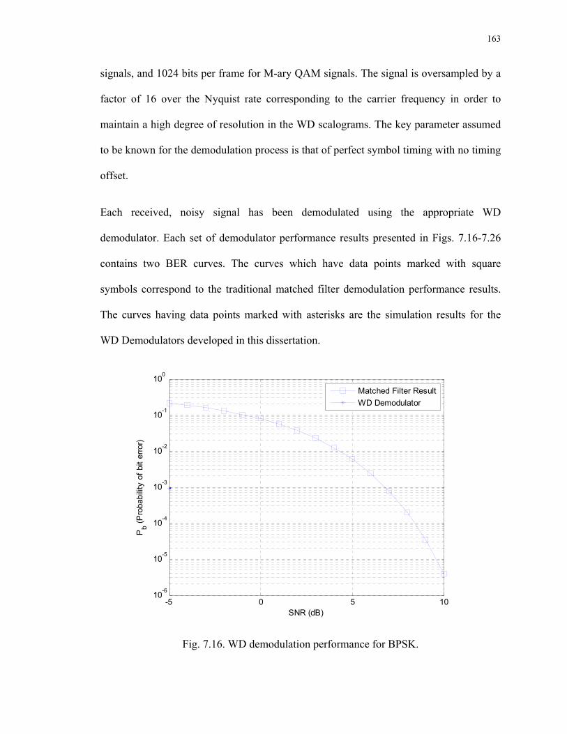
163
signals, and 1024 bits per frame for M-ary QAM signals. The signal is oversampled by a
factor of 16 over the Nyquist rate corresponding to the carrier frequency in order to
maintain a high degree of resolution in the WD scalograms. The key parameter assumed
to be known for the demodulation process is that of perfect symbol timing with no timing
offset.
Each received, noisy signal has been demodulated using the appropriate WD
demodulator. Each set of demodulator performance results presented in Figs. 7.16-7.26
contains two BER curves. The curves which have data points marked with square
symbols correspond to the traditional matched filter demodulation performance results.
The curves having data points marked with asterisks are the simulation results for the
WD Demodulators developed in this dissertation.
-5 0 5 1010-6
10-5
10-4
10-3
10-2
10-1
100
SNR (dB)
Pb (P
roba
bilit
y of
bit
erro
r)
Matched Filter ResultWD Demodulator
Fig. 7.16. WD demodulation performance for BPSK.
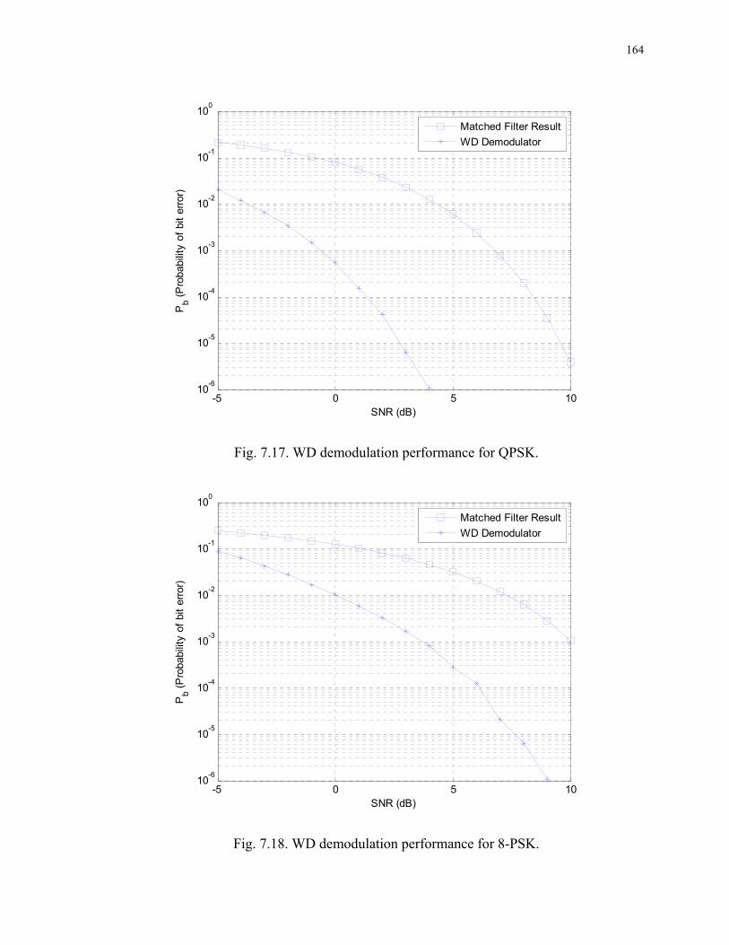
164
-5 0 5 1010-6
10-5
10-4
10-3
10-2
10-1
100
SNR (dB)
Pb (P
roba
bilit
y of
bit
erro
r)
Matched Filter ResultWD Demodulator
Fig. 7.17. WD demodulation performance for QPSK.
-5 0 5 1010-6
10-5
10-4
10-3
10-2
10-1
100
SNR (dB)
Pb (P
roba
bilit
y of
bit
erro
r)
Matched Filter ResultWD Demodulator
Fig. 7.18. WD demodulation performance for 8-PSK.

165
-5 0 5 1010-6
10-5
10-4
10-3
10-2
10-1
100
SNR (dB)
Pb (P
roba
bilit
y of
bit
erro
r)
Matched Filter ResultWD Demodulator
Fig. 7.19. WD demodulation performance for BASK.
-5 0 5 1010-6
10-5
10-4
10-3
10-2
10-1
100
SNR (dB)
Pb (P
roba
bilit
y of
bit
erro
r)
Matched Filter ResultWD Demodulator
Fig. 7.20. WD demodulation performance for 4-ASK.
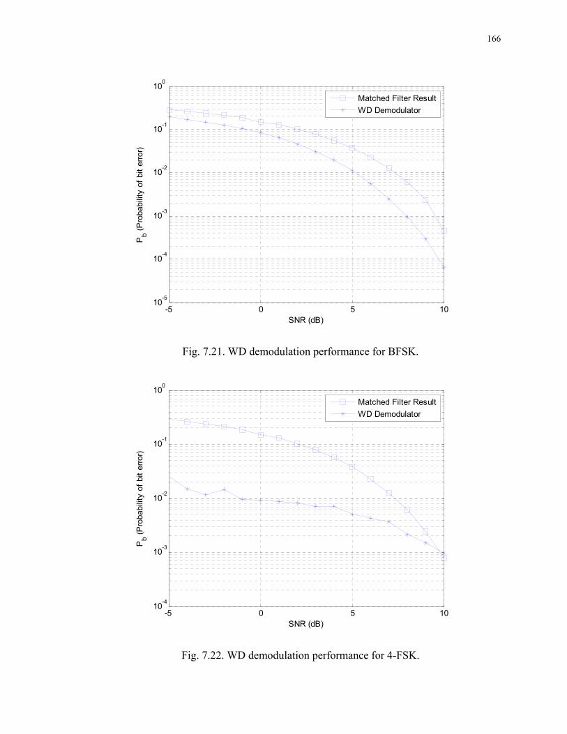
166
-5 0 5 1010-5
10-4
10-3
10-2
10-1
100
SNR (dB)
Pb (P
roba
bilit
y of
bit
erro
r)
Matched Filter ResultWD Demodulator
Fig. 7.21. WD demodulation performance for BFSK.
-5 0 5 1010-4
10-3
10-2
10-1
100
SNR (dB)
Pb (P
roba
bilit
y of
bit
erro
r)
Matched Filter ResultWD Demodulator
Fig. 7.22. WD demodulation performance for 4-FSK.

167
-5 0 5 1010-6
10-5
10-4
10-3
10-2
10-1
100
SNR (dB)
Pb (P
roba
bilit
y of
bit
erro
r)
Matched Filter ResultWD Demodulator
Fig. 7.23. WD demodulation performance for 4-QAM ( 4π -QPSK).
-5 0 5 1010-3
10-2
10-1
100
SNR (dB)
Pb (P
roba
bilit
y of
bit
erro
r)
Matched Filter ResultWD Demodulator
Fig. 7.24. WD demodulation performance for 16-QAM.

168
-5 0 5 1010-5
10-4
10-3
10-2
10-1
100
SNR (dB)
Pb (P
roba
bilit
y of
bit
erro
r)
Matched Filter ResultWD Demodulator
Fig. 7.25. WD demodulation performance for 64-QAM.
-5 0 5 1010-2
10-1
100
SNR (dB)
Pb (P
roba
bilit
y of
bit
erro
r)
Matched Filter ResultWD Demodulator
Fig. 7.26. WD demodulation performance for 256-QAM.

169
The BER curves obtained using the WD Demodulation techniques developed in this
dissertation are compared with BER curves corresponding to standard matched filter-
based demodulation in Figs. 7.16-7.26. It has been observed that the probability of error
is almost zero for BPSK signals for WD Demodulation using the common features
templates. The exception is when SNR= -5 dB where the BER is found to be Pb =
49.3 10−× . For the cases of QPSK and 8-PSK, the experimental BER curves based on WD
Demodulation are one or two orders of magnitude better than the matched filter-based
demodulation BER curves.
In the case of a BFSK signal, however, there is only slight improvement in performance
when WD Demodulation employing the common features templates is used as compared
to the matched filter-based BER curve. The BER curve corresponding to the WD
Demodulation of 4-FSK is, however, an order of magnitude better than the matched
filter-based BER curve for low SNR values, while the performances are comparable at
higher SNR values.
For 4-QAM signals, the BER curve obtained using WD Demodulation shows better
performance when compared with the matched filter-based BER curve at high SNR
values. However, there is only slight improvement in the experimental BER results
compared to the matched filter-based results for 16-QAM signals. For 64 QAM signals
the BERs are at least one order of magnitude smaller at high SNR values when WD
Demodulation is used as compared with traditional matched filtering. In the case of 256-
QAM signals both methods produce similar performance. This might be due to the
number of symbols employed in the demodulation simulations. The number of symbols
used per frame transmitted is 128 symbols in the demodulation of QAM signals. There

170
are 256 different symbols defined in a 256-QAM signal, therefore, increasing the number
of symbols per trial might yield improved BER performance for the WD Demodulator.
7.4 Discussion of Results
In this chapter two WD Demodulation methodologies have been described in detail. Both
the unique features templates and the common features templates have been used for WD
Demodulation of digitally modulated communications signals. The WD Demodulation
methodologies have also been devised in a manner such that automatic demodulation of a
communications signal is possible after the modulation scheme has been recognized by
the WD AMR processor. This feature, which ensures that a signal-specific demodulator
can be selected automatically, is advantageous for the development of agile radio
receivers.
The WD Demodulation methodology described in Section 7.1 based on unique features
templates is only useful for demodulating binary modulation schemes. The BER
performance of this methodology for the cases of BASK, BFSK and BPSK signals show
that only a few errors occur for SNR less than 0 dB. There is, however a drawback to this
method. If all data symbols transmitted are the same, then the probability of error could
either be unity, or zero. This is because the unique features templates are based on
symbol transitions, and no data changes were present to create symbol transitions in such
transmitted signals. In order to overcome this deficiency, an RZ data symbol format is
required to be implemented instead of an NRZ format used in this work.

171
The second WD Demodulation methodology described in Section 7.2 utilizes common
features templates, which are described based on the sinusoidal carrier within a symbol
period in a digitally modulated signal. The operation of cross-correlation in the wavelet-
domain between known templates and a received, noisy signal is again central to this
methodology. Based on the application of specific decision rules the baseband data are
recovered. Due to the variations of both amplitude and phase that occur in M-ary QAM
signals, additional templates are introduced in order to recognize the size of a particular
QAM signal. The additional templates are used for development of the decision rule for
the demodulation of M-ary signals. It is seen from Figs. 7.24-7.26 that the WD
Demodulator produces improved BER performance as compared to the traditional match
filter-based methods via Monte Carlo simulations.
For every modulation scheme considered in this dissertation, the WD Demodulation
methodologies performed better than traditional matched filter-based method. This
observation is based on comparing the BER performances obtained using both types of
demodulators. This trend is seen in the cases of WD Demodulation based on unique
features templates, as well as in the cases where common features templates are used.
The BER performance results of WD Demodulation for PSK signals are at least two to
three orders of magnitude better as compared to the traditional matched filter-based
methods at lower values of SNR. On the other hand, the WD Demodulator produced no
errors at SNR > -4 dB for BPSK signals; at SNR > 4 dB for QPSK signals; and at SNR >
9 dB for 8-PSK signals. For more complex modulation schemes, such as 16-, 64- and
256-QAM signals, the WD Demodulator BER performance for the 16-QAM signal
shows slight improvement over the matched filter-based method. In the case of a 64-
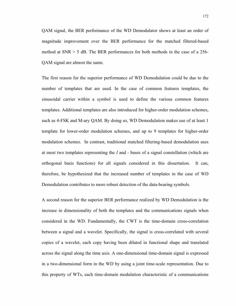
172
QAM signal, the BER performance of the WD Demodulator shows at least an order of
magnitude improvement over the BER performance for the matched filtered-based
method at SNR > 5 dB. The BER performances for both methods in the case of a 256-
QAM signal are almost the same.
The first reason for the superior performance of WD Demodulation could be due to the
number of templates that are used. In the case of common features templates, the
sinusoidal carrier within a symbol is used to define the various common features
templates. Additional templates are also introduced for higher-order modulation schemes,
such as 4-FSK and M-ary QAM. By doing so, WD Demodulation makes use of at least 1
template for lower-order modulation schemes, and up to 9 templates for higher-order
modulation schemes. In contrast, traditional matched filtering-based demodulation uses
at most two templates representing the I and - bases of a signal constellation (which are
orthogonal basis functions) for all signals considered in this dissertation. It can,
therefore, be hypothesized that the increased number of templates in the case of WD
Demodulation contributes to more robust detection of the data-bearing symbols.
A second reason for the superior BER performance realized by WD Demodulation is the
increase in dimensionality of both the templates and the communications signals when
considered in the WD. Fundamentally, the CWT is the time-domain cross-correlation
between a signal and a wavelet. Specifically, the signal is cross-correlated with several
copies of a wavelet, each copy having been dilated in functional shape and translated
across the signal along the time axis. A one-dimensional time-domain signal is expressed
in a two-dimensional form in the WD by using a joint time-scale representation. Due to
this property of WTs, each time-domain modulation characteristic of a communications
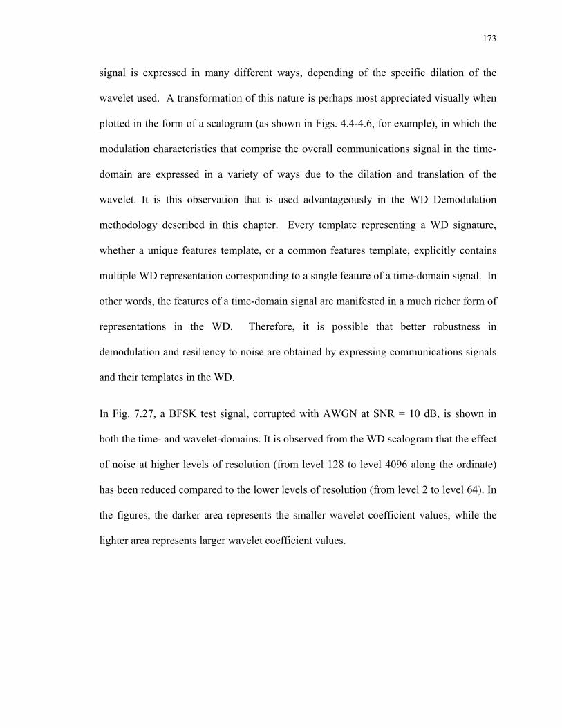
173
signal is expressed in many different ways, depending of the specific dilation of the
wavelet used. A transformation of this nature is perhaps most appreciated visually when
plotted in the form of a scalogram (as shown in Figs. 4.4-4.6, for example), in which the
modulation characteristics that comprise the overall communications signal in the time-
domain are expressed in a variety of ways due to the dilation and translation of the
wavelet. It is this observation that is used advantageously in the WD Demodulation
methodology described in this chapter. Every template representing a WD signature,
whether a unique features template, or a common features template, explicitly contains
multiple WD representation corresponding to a single feature of a time-domain signal. In
other words, the features of a time-domain signal are manifested in a much richer form of
representations in the WD. Therefore, it is possible that better robustness in
demodulation and resiliency to noise are obtained by expressing communications signals
and their templates in the WD.
In Fig. 7.27, a BFSK test signal, corrupted with AWGN at SNR = 10 dB, is shown in
both the time- and wavelet-domains. It is observed from the WD scalogram that the effect
of noise at higher levels of resolution (from level 128 to level 4096 along the ordinate)
has been reduced compared to the lower levels of resolution (from level 2 to level 64). In
the figures, the darker area represents the smaller wavelet coefficient values, while the
lighter area represents larger wavelet coefficient values.
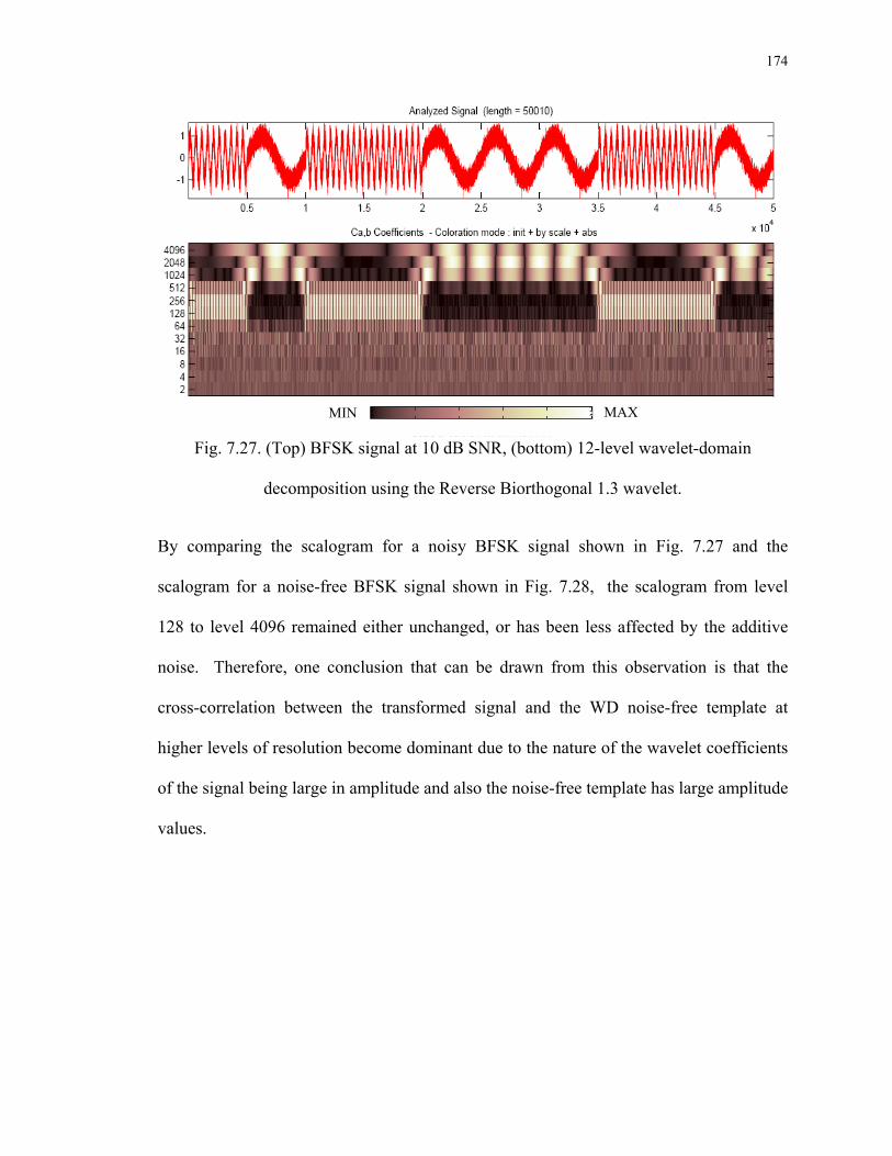
174
Fig. 7.27. (Top) BFSK signal at 10 dB SNR, (bottom) 12-level wavelet-domain
decomposition using the Reverse Biorthogonal 1.3 wavelet.
By comparing the scalogram for a noisy BFSK signal shown in Fig. 7.27 and the
scalogram for a noise-free BFSK signal shown in Fig. 7.28, the scalogram from level
128 to level 4096 remained either unchanged, or has been less affected by the additive
noise. Therefore, one conclusion that can be drawn from this observation is that the
cross-correlation between the transformed signal and the WD noise-free template at
higher levels of resolution become dominant due to the nature of the wavelet coefficients
of the signal being large in amplitude and also the noise-free template has large amplitude
values.
MIN MAX
175
Fig. 7.28 (Top) BFSK signal without noise, (bottom) 12-level wavelet-domain
decomposition using the Reverse Biorthogonal 1.3 wavelet.
The third reason for better BER performance results obtained using the WD Demodulator
is due to the larger values of cross-correlation that exist between the best-matched
wavelet and the known modulation type signal at higher levels of resolution. The WD
Demodulation algorithm developed in this work is based on cross-correlation values
being compared with a fixed threshold value. Therefore, due to this observation, the
effect of noise on the cross-correlation values has been reduced which provides an
improvement in the BER performance as compared to the traditional matched filter-based
demodulation method.
MIN MAX

176
Chapter 8
Summary and Conclusions
8.1 Summary
The WD AMR algorithms invented in this dissertation are based on the cross-correlation
of received, noisy digitally modulated communications signals with WD signatures
corresponding to a known set of modulation schemes. The WD signatures are represented
as templates obtained from noise-free digitally modulated signals. Two categories of WD
signatures are defined, namely the unique features templates and the common features
templates. The unique features contain the symbol transition characteristics of a
communications signal. Each feature is unique to a particular digital modulation scheme.
Therefore, for higher-order modulation schemes, more unique features templates are
needed. Due to that fact, the computational effort increased.
The common features templates represent the sinusoidal carrier characteristics present
within a symbol period of a communications signal. Therefore, fewer numbers of
templates are needed for the WD AMR process. For example, only 28 common features
templates are needed to recognize 256-QAM signals as compared to the need for a total
of 65536 unique features templates otherwise.
The rates of correct classification reported in Chapter 4 show that all results are better
than those reported in the literature. The only drawback when using the unique features
templates is that because the templates are extracted so as to capture the symbol transition
characteristics, the WD AMR process might not able to recognize the particular
177
modulation scheme when the communications signal data sequences contain either all
data “1” or data “0” symbols.
The WD Demodulation method developed in this work is also based on the cross-
correlation of the WD signatures with received, noisy communications signals. It was
shown in Chapter 7 that the BER performance of the WD Demodulation process offers an
improvement over the traditional matched filtering method. The WD Demodulation
process is the first such methodology devised in the context of WTs.
Both the WD AMR and Demodulation processes devised in this dissertation are based on
the cross-correlation operations and feature extractions of signatures templates. Both
processes developed in this dissertation are based on a blind recognition technique. Other
methods, i.e., SVMs and ANNs, reported in the literature are use to enhance the
classification performance. However, they required a training sequence in order for the
sub-system to adapt to specific modulation scheme. Use of a training sequence further
increases the complexity and the computational effort of an AMR system. On the other
hand, the WD AMR and WD Demodulation processes developed in this work use
signatures templates and do not require the use of a training sequences.
8.2 Contributions of the Dissertation
Several key contributions of this work include:
1. Identification of WD signatures for the sets of modulation schemes considered in
this work. Development and construction of two WD signatures categories,
namely the unique features templates and the common features templates.

178
2. Development of techniques for choosing the best-suited wavelet(s) for use in both
the WD AMR and the WD Demodulation processes.
3. Development of two WD AMR algorithms using WD signatures of digitally
modulated communications signals.
4. Development of WD Demodulation algorithms using WD signatures of digitally
modulated communications signals.
5. Introduction of a new concept to be used for constructing templates for the
recognition of M-ary QAM signals.
6. Development of new techniques for recognizing different sizes of signal
constellations for M-ary QAM signals. The techniques are used in both the WD
AMR and the WD Demodulation processes.
7. Development and demonstration of the first WD Demodulation algorithm in the
context of WTs.
8.3 Applications
With the observations and results obtained for both the WD AMR and the WD
Demodulation algorithms, the ultimate goal of this dissertation work is to enable the
development of a Wavelet Platform as illustrated in Fig. 1.4 of Section 1.1. Such a signal
processing platform can be used to advance the state-of-the-art for communications
receiver design so as to permit interoperability between a variety of communications
standards. This type of receiver can be used in military signal analysis applications, such
as threat analysis, spectrum management, electronic warfare, and electronics surveillance
system.

179
Some of the potential application scenarios are presented below:
Application Scenario #1: Reconfigurable Radios in Hostile Environments
Communications systems that are ideally suited to hostile environments, such as those
encountered in battlefield conditions, can be developed with the use of the Wavelet
Platform. Such systems would feature rugged signal identification and demodulation
capabilities, the ability to de-noise received passband signals after characterization of the
noise process, and the ability to continuously compensate for channel fading
characteristics using adaptive channel equalization in the WD.
Application Scenario #2: Underwater Acoustic Communications
A key feature of the Wavelet Platform is that a wide variety of signals, noise, or channel
fading characteristics can be analyzed. Such analysis is very useful in communications
systems that transport data via acoustic signals, as is the case in underwater acoustic
communications. Time and spatially varying channel conditions can be identified,
tracked, and exploited to recover data in digitally modulated signals employed in
underwater communications systems.
8.4 Suggestions for Future Work
The research work in this dissertation involved the development of WD AMR and WD
Demodulation algorithms. The methodologies used for both processes represent a
relatively new area as compared to the work reported in the literature. Therefore, the
research activities pursued in connection with this dissertation have opened many new
directions that can be further explored.
180
Both the WD AMR and WD Demodulation processes require that a preliminary setup
procedure be performed. The initial tasks involve the construction of WD signatures in
the form of scalogram templates and selection of a suitable wavelet to be used for both
the construction of the WD signatures and the transformation of the received
communications signals via the CWT.
A natural extension of the work described in this dissertation is to improve upon the
correct classification rates for the WD AMR process by using different wavelets. It has
been observed that certain wavelets easily highlight the unique features of particular
communications signals that employ variations in carrier amplitude, frequency, or phase.
Based on the results obtained in Figs. 4.30 and 4.32, it seems reasonable that by using a
different wavelet for each distinguishing feature contained in a particular type of
modulation scheme, especially in the case of FSK signals, the rate of correct
classification, and also the quality of the demodulation accuracy, may be improved. The
use of different and/or multiple wavelets for extraction of key features of digital signals
corresponding to particular modulation schemes can enable the development of a Hybrid
WD AMR method.
The WD AMR and WD Demodulation processes can also be expanded to include other
communications signals such as Gaussian Minimum Shift Keying (GMSK), and non-
square M-ary QAM signal constellations.
Also, this research work has limited attention to communications signals that have been
corrupted with zero-mean AWGN. System performance assessment could be exteneded
181
to other noise scenarios such as impulsive noise (of different bandwidth), band-limited
noise, etc.
The communications signals were oversampled by a factor of sixteen over the Nyquist
rate in relation to the carrier frequency in this work. Further investigation aimed at
reducing the number of samples within a symbol is warranted. Additional reduction in
computational effort may be possible. However, it is important to assess the affect on the
overall modulation classification rate and also the BER performance of the demodulator.
Having demonstrated the efficacy of the developed WD AMR process and the WD
Demodulation process, these processes can be implemented in hardware. The algorithms
developed for WD AMR and WD Demodulation can both be realized using Field
Programmable Gate Array (FPGA) technology for use in a radio receiver system.
Therefore, a WD-based radio receiver can be demonstrated using an FPGA prototype.
Based on the definitions of the decision rules and the algorithms for the WD
Demodulation process, a theory can be developed so as to predict the demodulation
performance. The procedural steps in development of such a theory should be parallel to
the steps taken in the development of the matched filter theory describing the matched
filter performance.
8.5 Conclusions
In this work, it has been demonstrated that with the use of the pattern recognition
methodology of template matching, along with appropriately defined WD templates, both
the AMR and demodulation processes can be implemented in the WD. It has been
182
demonstrated that the WD AMR process can correctly classify modulation schemes with
very high reliability even for low values of SNR. At SNR = -5 dB, the correct
classification rates are 100% for both BPSK and 8-PSK signals, 94.7% for QPSK signals,
and above 95% for BASK as well as 4-ASK signals. The rates of correct classification
are 100% for both 16-QAM and 256-QAM signals, and 96.1% for 64-QAM signals.
These results meet, or exceed, those reported in the literature for other AMR schemes.
Furthermore, it has also been demonstrated that the WD Demodulator provides
improvement in BER performance over the traditional matched filter-based methods. In
particular, a few orders of magnitude of improvement is seen for PSK signals, while
approximately equal performances are obtained for M-ary QAM signals.
Given the reliability of both the WD AMR and WD Demodulation processes devised in
this work, they can be used to advance the state-of-the-art of communications receiver
design, more specifically, by enabling the development of a Wavelet Platform. The
Wavelet Platform provides the agility to permit interoperability between different
communications standards to subsequent automatic demodulation with a single
demodulator.

183
References
1. Vaz, C. and Ho, K. M., "Development of Adaptive Radio Transceivers," Technical Report 06/09, Dept. Elect. Comput. Eng., Rutgers, The State University of New Jersey, Piscataway, NJ, June 2009.
2. Vaz, C. and Ho, K. M., "Illustrative Conceptualization of the Wavelet Platform," Technical Report 07/09, Dept. Elect. Comput. Eng., Rutgers, The State University of New Jersey, Piscataway, NJ, July 2009.
3. IEEE 802.11a-1999 Standard. (2007, October). [Online]. Available: http://standards.ieee.org/getieee802/802.11.html
4. ZigBee Specification Document 053474r13. (2007, October). [Online]. Available: http://www.zigbee.org/en/
5. IEEE 802.11b-1999 Standard. (2007, October). [Online]. Available: http://standards.ieee.org/getieee802/802.11.html
6. Bluetooth Specification Version 2.1 + EDR [vol 0]. (2007, October). [Online]. Available: http://www.bluetooth.com/Bluetooth/Learn/Technology/Specifications/
7. ETSI EN 300 744 V1.5.1 (2004-11). Digital Video Broadcasting (DVB); Framing Structure, Channel Coding and Modulation for Digital Terrestrial Television. (2007, October). [Online]. Available: http://www.etsi.org/WebSite/Standards/Standard.aspx
8. American National Standard ANSI/SCTE 07 2006. Digital Transmission Standard for Cable Television. (2007, October). [Online]. Available: http://www.scte.org/content/index.cfm?pID=102
9. Dobre, O. A., Abdi, A., Bar-Ness, Y. and Su, W., “A Survey of Automatic Modulation Classification Techniques: Classical Approaches and New Trends,” IET Comm., Vol. 1, Issue 2, pp. 137-157, Apr. 2007.
10. Abrahamzadeh, A., Seyedin, S. A. and Dehghan, M., "Digital-Signal-Type Identification Using an Efficient Identifier," EURASIP Journal on Advances in Signal Processing, Vol. 2007, 2007.
11. Ebrahimzadeh, A. and Seyedin, S. A., "Digital Signal Types Identification Using a Hierarchical SVM-Based Classifier and Efficient Features,” Proc. 2007 Int. Conf. Computing: Theory and Applications, pp. 521-525, Mar. 2007.
12. Wu, Z. Wang, X., Gao, Z. and Ren, G., "Automatic Digital Modulation Recognition Based on Support Vector Machines," Proc. 2005 Int. Conf. on Neural Networks and Brain, Vol. 2, pp. 1025- 1028, Oct. 2005.
184
13. Han, G., Li, J. and Lu, D., "Study of Modulation Recognition Based on HOCs and SVM," Proc. 59th Vehicular Tech. Conf., Vol. 2, pp. 898- 902, May 2004.
14. Richterova, M., "Signal Modulation Recognizer Based on Method of Artificial Neural Networks," Proc. 2005 Progress in Electromagnetics Research Symp., pp. 575-578, Aug. 2005.
15. Yang, C.-Q., Zhong, Z.-F. and Yang, J.-A., "Recognition of Digital Modulation Using Radial Basis Function Neural Networks," Proc. 2003 Int. Conf. Machine Learning and Cybernetics, Vol. 5, pp. 3012- 3015, Nov. 2003.
16. Zhao, Y., et al., "Automatic Digital Modulation Recognition Using Artificial Neural Networks," Proc. 2003 Int. Conf. on Neural Networks and Signal Processing, Vol. 1, pp. 257-260, Dec. 2003.
17. Wong, M. L. D. and Nandi, A. K., "Automatic Digital Modulation Recognition Using Spectral Andstatistical Features With Multi-Layer Perceptrons," Proc. Sixth International Symp. Signal Processing and its Applications, Vol. 2, pp. 390-393, Aug. 2001.
18. Chen, J., et al., "Digital Modulation Identification Based on Software Radio Platform," Proc. Sixth Int. Conf. Parallel and Distributed Computing, Applications and Technologies, pp. 945- 949, Dec. 2005.
19. Dobre, O. A., Abdi, A., Bar-Ness, Y. and Su, W., "Blind Modulation Classification: A Concept Whose Time Has Come," Proc. 2005 IEEE/Sarnoff Symp. on Advances in Wired and Wireless Comm., pp. 223-228, Apr. 2005.
20. Li, J., He, C. and Chen, J., "Automatic Digital Modulation Identification Basing on Decision Method and Cumulants," Proc. 2005 IEEE Int. Workshop VLSI Design and Video Tech., pp. 264- 267, May 2005.
21. Pedzisz, M. and Mansour, A., "Automatic Modulation Recognition of MPSK Signals Using Constellation Rotation and its 4th Order Cumulant," Digital Signal Processing, Vol. 15, Issue 3, pp. 295-304, May 2005.
22. Wang, B. and Ge, L., "Blind Identification of OFDM Signal in Rayleigh Channels," Proc. Fifth Int. Conf. on Information, Comm. and Signal Processing, pp. 950- 954, Dec. 2005.
23. Wu, Y.-X., Ge, L.-D. and Liu, F.-F., "Comprehensive Features Based Digital Modulation Identification Using a Neural Tree Network," Proc. 2005 Int. Conf. on Communications, Circuits and Systems, Vol. 2, pp. 748-752, May 2005.
24. Cai, Q., Wei, P. and Xiao, X., "A Digital Modulation Recognition Method," Proc. Int. Conf. Communications, Circuits and Systems, Vol. 2, pp. 863- 866, Jun. 2004.
25. Hong, L. and Ho, K. C., "Classification of BPSK and QPSK Signals with Unknown
185
Signal Level Using the Bayes Technique," Proc. 2003 International Symposium on Circuits and Systems, Vol. 4, pp. 1- 4, May 2003.
26. Le Guen, D. and Mansour, A., "Automatic Recognition Algorithm for Digitally Modulated Signals," Proc. IASTED Int. Conf. on Signal Processing, Pattern Recognition and Applications, pp. 32-37, Jun. 2002.
27. Hong, L. and Ho, K. C., "Modulation Classification of BPSK and QPSK Signals Using a Two Element Antenna Array Receiver," Proc. 2001 Mil. Comm. Conf., Vol. 1, pp. 118- 122, 2001.
28. Boudreau, D., et al., "A Fast Automatic Modulation Recognition Algorithm and Its Implementation in a Spectrum Monitoring Application," Proc. 21st Century Mil. Comm. Conf., Vol. 2, pp. 732-736, Oct. 2000.
29. Taira, S., “Automatic Classification of QAM Signals in Fading Channel,” Proc. 51st Vehicular Tech. Conf., Vol. 3, pp. 1717-1721, May 2000.
30. Chan, Y., Gadbois, L. and Yansouni, P., "Identification of the Modulation Type of a Signal," Proc. 1985 IEEE Int. Conf. on Acoustics, Speech, and Signal Processing, Vol. 10, pp. 838- 841, Apr. 1985.
31. Nagy, P. A. J., "A Modulation Classifier for Multi-Channel Systems and Multi-Transmitter Situations," Conf. IEEE Mil. Comm. Conf., Vol. 3, pp. 816 - 820, Oct. 1994.
32. Azzouz, E. E. and Nandi, A. K., “Automatic Identification of Digital Modulation Types,” Signal Processing, Vol. 47, No. 1, pp. 55-69, 1995.
33. Soliman, S. S. and Hsue, S.-Z., "Signal Classification Using Statistical Moments," IEEE Trans. Comm., Vol. 40, No. 5, pp. 908-916, May 1992.
34. Nandi, A. K. and Azzouz, E. E., "Algorithms for Automatic Modulation Recognition of Communication Signals," IEEE Trans. Commum., Vol. 46, No. 4, pp. 431-436, April 1998.
35. Azzouz, E. E. and Nandi, A. K., "Procedure for Automatic Recognition of Analogue and Digital Modulations," IEE Proc.-Communications, Vol. 143, Issue 5, pp. 259-266, Oct. 1996.
36. Park, C.-S., Jang, W., Nah, S.-P. and Kim, D. Y., "Automatic Modulation Recognition using Support Vector Machine in Software Radio Applications," Proc. 9th Int. Conf. Advanced Communication Tech., Vol. 1, pp. 9-12, Feb. 2007.
37. Feng, X. Z., Yang, J., Luo, F. L., Chen, J. Y. and Zhong, X. P., "Automatic Modulation Recognition by Support Vector Machines Using Wavelet Kernel," J. Phys.: Conf. Ser., Vol. 48, pp. 1264-1267, 2006.
186
38. Hossen, A., Al-Wadahi, F. and Jervase, J. A., “Classification of Modulation Signals Using Statistical Signal Characterization and Artificial Neural Networks,” Engineering Applications of Artificial Intelligence, Vol. 20, Issue 4, pp. 463-472, Jun. 2007.
39. Kamarthi. S. V., Zeid, I. and Subramaniam, L., "Multiresolution Approach to Identification of Recurring Signal Patterns," Proc. SPIE, Wavelet Applications in Industrial Processing IV, Vol. 6383, Oct. 2006.
40. Rashid, I., Maqbool, H., Mehmood-ur-Rehman and Nadir, F., "Digital Modulation Identification by Basic Modulation Parameters," Proc. 9th Int. Multioptic Conference, pp. 1-6, Dec. 2005.
41. Shahmohammadi, M. and Nikoofar, H. R., "Modulation Classification for QAM/PSK Using a Soft Clustering Algorithm," Proc. 2002 IEEE Int. Symp. Info. Theory, p. 19, 2002.
42. Lopatka, J. and Pedzisz, M., "Automatic Modulation Classification Using Statistical Moments and a Fuzzy Classifier," Proc. 5th Int. Conf. on Signal Processing, Vol. 3, pp. 1500-1506, Aug. 2000.
43. Al-Jalili, Y. O., “Identification Algorithm of Upper Sideband and Lower Sideband SSB Signals," Signal Processing, Vol. 42, No. 2, pp. 207-213, 1995.
44. Martin, A., "A Signal Analysis and Classification Strategy for Implementation in an EW Communications Receiver," Proc. Fifth International Conference on Radio Receivers and Associated Systems, pp. 222-226, Jul. 1990.
45. Liedtke, F. F., "Computer Simulation of an Automatic Classification Procedure for Digitally Modulated Communication Signals with Unknown Parameters," Signal Processing, Vol. 6, Issue 4, pp. 311-323, August 1984.
46. Jondral, F., "Automatic Classification of High Frequency Signals," Signal Processing, Vol. 9, Issue 3, pp. 177 - 190, Oct. 1985.
47. Park, C., Choi, J., Nah, S., Jang, W. and Kim, D.Y., “Automatic Modulation Recognition of Digital Signals using Wavelet Features and SVM,” 10th Int. Conf. Advanced Comm. Tech., Vol. 1, pp. 387-390, February 2008.
48. Prakasam, P. and Madheswaran, M., “Automatic Modulation Identification of QPSK and GMSK Using Wavelet Transform for Adaptive Demodulator in SDR,” IEEE Int. Conf. Signal Process., Comm. and Networking, pp. 507-511, Feb. 2007.
49. Feng, X. Z., Yang, J., Luo, F. L., Chen, J. Y. and Zhong, X. P., “Automatic Modulation Recognition by Support Vector Machines Using Wavelet Kernel,” J. Phy. Conf. Series, Vol. 48, Issue 1, pp. 1264-126, 2006.
50. Wei, X. and Cao, Z., “Fast Identification of Amplitude Modulated Signals at Low
187
SNR,” IEEE Int. Symp. Microwave, Antenna, Propagation and EMC Tech. Wireless Comm., Vol. 2, pp. 1119-1112, Aug. 2005.
51. Chen, J., Kuo, Y., Li, J., Fu, F. and Ma, Y., “Digital Modulation Identification by Wavelet Analysis,” Proc. 6th Int. Conf. Computational Intelligence and Multimedia Application, pp. 29-34, Aug. 2005.
52. Pavlik, R., “Binary PSK/CPFSK and MSK Bandpass Modulation Identifier Based on the Complex Shannon Wavelet Transform,” J. Elect. Eng., Vol. 56, No. 3-4, pp. 71-77, 2005.
53. Ou, X., Huang, X., Yuan, X. and Yang, W., “Qusai-Haar Wavelet and Modulation Identification of Digital Signals,” IEEE Int. Conf. Comm. Circuits and Systems, Vol. 2, pp. 733-737, Jun. 2004.
54. Jin, J-D., Kwak, Y., Lee, K-W., Lee, K. H. and Ko, S-J., “Modulation Type Classification Method using Wavelet Transform for Adaptive Modulator,” IEEE Proc. Int. Symp. Intelligent Signal Processing and Communication Systems, pp. 282-292, Nov. 2004.
55. Hippenstel, R., El-Kishky, H., Frick, C. and Datasprasad, S., “Modulation Identification using Neural Network and Wavelet Domain Based Approaches,” IEEE 38th Asilomar Conf. Signals, Systems and Computers, Vol. 2, pp. 2116-2120, Nov. 2004.
56. Zeng, X., Tan, X. and Liu, J., “PN Code Acquisition Detection for CDMA Networks Based on Wavelet Transform and Artificial Neural Network,” IEEE Proc. Int. Conf. Wavelet Anal. and Its Applicat., Vol. 2, pp. 1524-1527, Apr. 2003.
57. Wilson, S. S., “Using a Pseudo-random Binary Sequence as a Mother Wavelet in the Wavelet-correlation System Identification Method,” IEEE Proc. SoutheastCon, pp. 58-61, Apr. 2002.
58. Ho, K. C., Prokopiw, W. and Chan, Y.T., “Modulation Identification of Digital Signals by the Wavelet Transform,” Proc. IEE – Radar, Sonar, and Navigation, Vol. 147, pp. 169-176, Aug. 2000.
59. Liu, H., and Ho, K. C., “Identification of CDMA Signal and GSM Signal Using the Wavelet Transform”, IEEE 42nd Midwest Symp. on Circuits and Systems, Vol. 2, pp. 678-681, Aug. 1999.
60. Hong, L. and Ho, K. C., “Identification of Digital Modulation Types using the Wavelet Transform,” Mil. Comm. Conf. Proc., Vol. 1, pp. 427-431, Nov. 1999.
61. Ho, K. C., Liu, H., and Hong, L., “On Improving the Accuracy of a Wavelet Based Identifier to Classify CDMA Signal and GSM Signal”, Proc. IEEE International Symp. on Circuits and Systems VLSI, Vol. 4, pp. 564-567, 1999.
188
62. Ho, K. C., Prokopiw, W. and Chan, Y. T., “Modulation Identification by the Wavelet Transform,” Mil. Comm. Conf. Proc., Vol. 2, pp. 886-890, Nov. 1995.
63. Zhang, D. and Wang, X., “MPSK Modulation Recognition Based on Wavelet Transformation,” Int. Conf. on Networking and Dig. Society, Vol. 1, pp. 202-205, May 2009.
64. Chen, G., Ren, Z. and Li, Y., “Study of Signal Feature Recognition Method Based on Morlet Combined Wavelets,” Int. Conf. Measuring Tech. Mech. Automation, pp. 313-317, April, 2009.
65. Mallat, S., A Wavelet Tour of Signal Processing, Second Edition, Academic Press, San Diego, CA, 1999.
66. Turin, G. L., “An Introduction to Matched Filters”, IRE Trans. Info. Theory, Vol. 6, pp. 311-329, Jun. 1960.
67. Turin, G. L., “An Introduction to Matched Filters”, Proc. of IEEE, Vol. 64, pp. 1092-1112, Jul. 1976.
68. Bruce, A. G., Gao, H., Mulligan, J. J. and Satrius, E. H., “Application of Wavelet De-Noising to Signal Demodulation,” IEEE 29th Asilomar Conf. Signals, Systems and Computer, Vol. 2, pp. 1142-1146, Nov. 1995.
69. Ho, K. M., Vaz, C. and Daut, D. G., “Improved Demodulation of Phase Shift Keyed Signals Using Wavelet Thresholding,” 2008 IEEE Sarnoff Symposium, Princeton, NJ, USA, pp. 1-6, April 2008.
70. Daubechies, I., Ten Lectures on Wavelets, Eighth Printing, Society for Industrial and Applied Mathematics, Philadelphia, PA, 2004.
71. Beylkin, G., Coifman, R. and Rokhlin, V., “Fast Wavelet Transforms and Numerical Algorithms,” Comm. Pure Applied Math., Vol. 44, Issue 2, pp. 141-183, 1991.
72. Grossmann, A. and Morlet, J., “Decomposition of Hardy Functions into Square Integrable Wavelets of Constant Shape,” SIAM J. Math. Analysis, Vol. 15, Issue 4, pp. 723-736, July 1984.
73. Mallat, S., “Multiresolution Approximation and Wavelet Orthogonal Bases of L2,” Trans. AMS, Vol. 315, No. 1, pp. 69-87, September 1989.
74. Bracewell, R. N., The Fourier Transform and Its Applications, McGraw-Hill, New York, NY, 1986.
75. Daubechies, I., "The Wavelet Transform, Time-Frequency Localization and Signal Analysis," IEEE Trans. Inf. Theory, Vol. 36, No. 5, pp. 961-1005, September 1990.
76. Sarkar, T. K., el. al, “A Tutorial on Wavelets from an Electrical Engineering Perspective, Part 1: Discrete Wavelet Techniques,” IEEE Trans. Antennas Propag. Mag., Vol. 40, No. 5, pp. 49-68, October 1998.
189
77. Poularikas, A. D., Ed., The Transforms and Applications Handbook, CRC Press, Boca Raton, FL, 1996.
78. Benedetto, J. J. and Frazier, M. W., Wavelets: Mathematics and Applications, CRC Press, Inc., Boca Raton, FL, 1994.
79. Rao, R. M. and Bopadrikar, A. S., Wavelet Transforms, Addison-Wesley, Reading, MA, 1998.
80. Wickerhauser, M. V., Adapted Wavelet Analysis from Theory to Software, A. K. Peters, Ltd., Wellesley, MA, 1994.
81. Jansen, M., Noise Reduction by Wavelet Thresholding, Springer-Verlag, New York, NY, 2001.
82. Oppenheim, A. V., Schafer, R. W. and Buck, J. R., Discrete-Time Signal Processing, Second Edition, Prentice Hall, Upper Saddle River, NJ, 1999.
83. Mallat, S., A Wavelet Tour of Signal Processing, Second Edition, Academic Press, San Diego, CA, 1999.
84. Proakis, J. G., Digital Communications, Fourth Edition, McGraw-Hill, NY, NY, 2001.
85. Ho, K. M., Vaz, C. and Daut, D. G., “A Wavelet-Based Method for Classification of Binary Digitally Modulated Signals,” 2009 IEEE Sarnoff Symposium, pp. 1-5, March 2009.
86. Azzouz, E. E. and Nandi, A. K., Automatic Modulation Recognition of Communication Signals, First Edition, Kluwer Academic Publishers, Dordrecht, The Netherlands,1996.
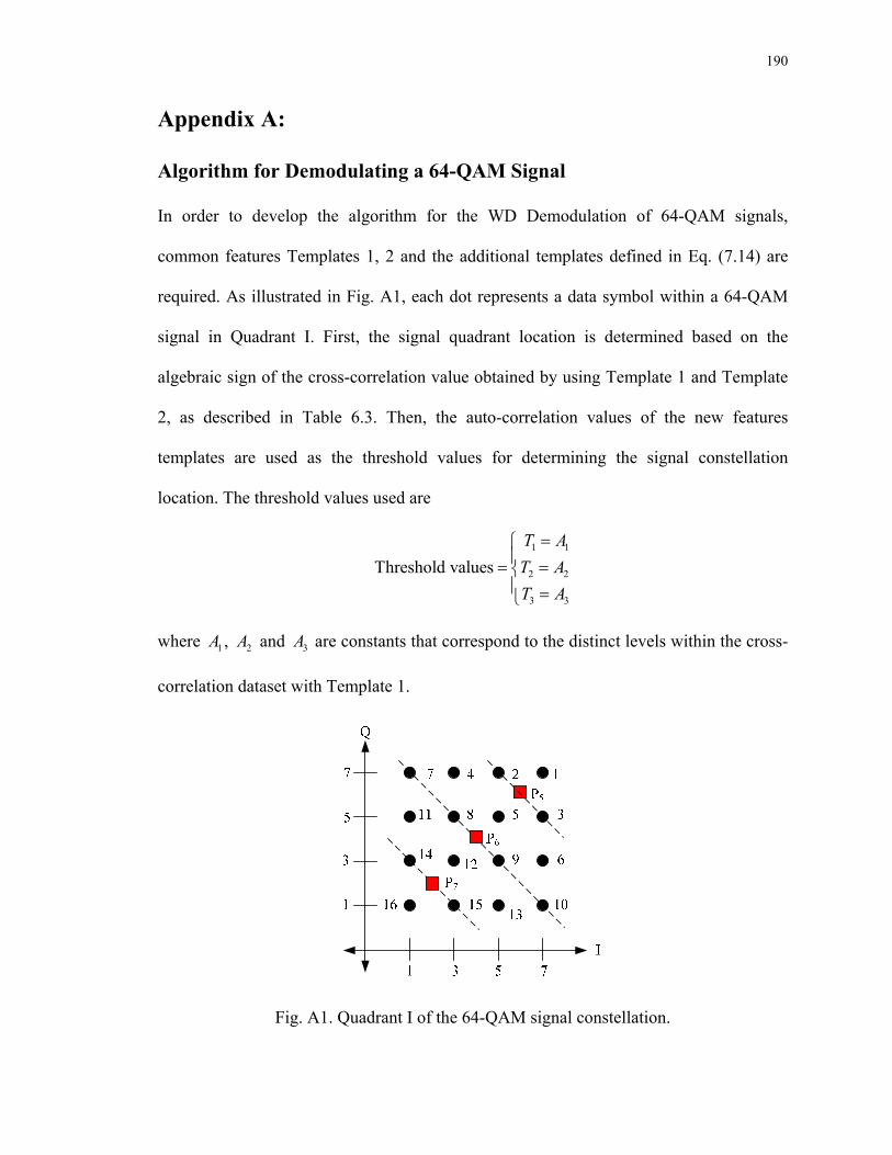
190
Appendix A:
Algorithm for Demodulating a 64-QAM Signal
In order to develop the algorithm for the WD Demodulation of 64-QAM signals,
common features Templates 1, 2 and the additional templates defined in Eq. (7.14) are
required. As illustrated in Fig. A1, each dot represents a data symbol within a 64-QAM
signal in Quadrant I. First, the signal quadrant location is determined based on the
algebraic sign of the cross-correlation value obtained by using Template 1 and Template
2, as described in Table 6.3. Then, the auto-correlation values of the new features
templates are used as the threshold values for determining the signal constellation
location. The threshold values used are
1 1
2 2
3 3
Threshold valuesT AT AT A
=⎧⎪= =⎨⎪ =⎩
where 1A , 2A and 3A are constants that correspond to the distinct levels within the cross-
correlation dataset with Template 1.
Fig. A1. Quadrant I of the 64-QAM signal constellation.
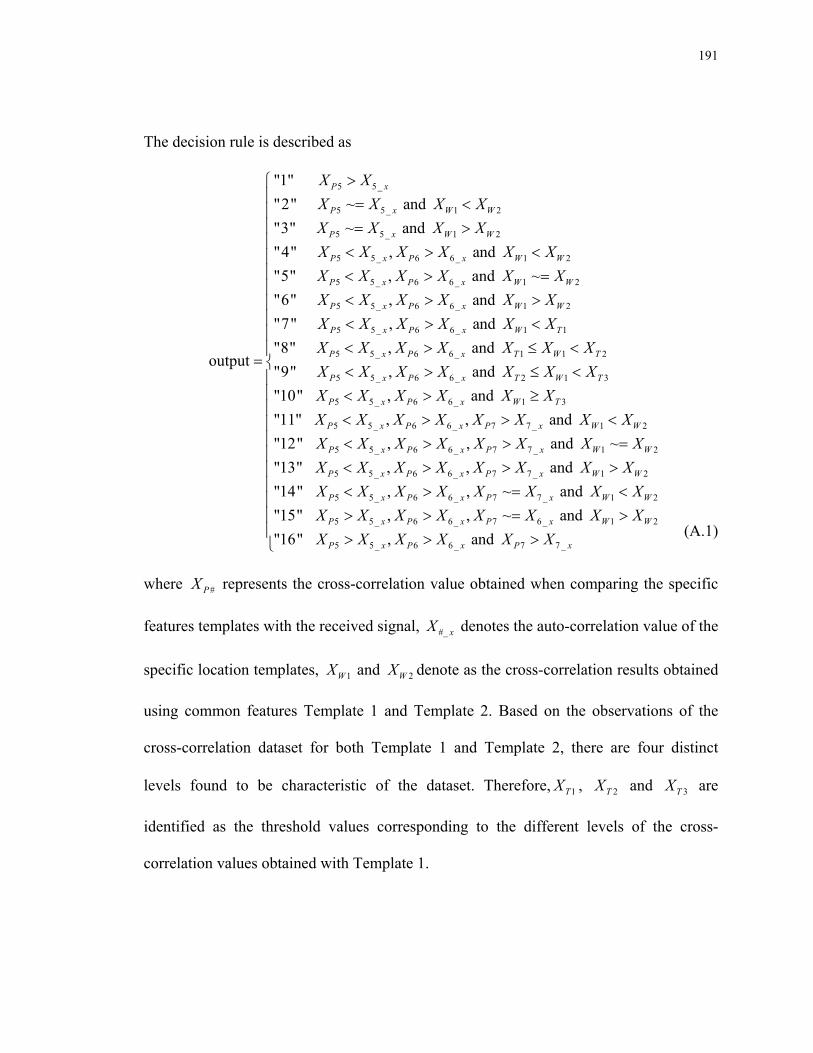
191
The decision rule is described as
5 5_
5 5_ 1 2
5 5_ 1 2
5 5_ 6 6 _ 1 2
5 5_ 6 6_ 1 2
5 5_ 6 6_ 1
"1" "2" ~ and "3" ~ and "4" , and "5" , and ~"6" , and
output
P x
P x W W
P x W W
P x P x W W
P x P x W W
P x P x W
X XX X X XX X X XX X X X X XX X X X X XX X X X X
>= <= >
< > << > =< > >
=
2
5 5_ 6 6 _ 1 1
5 5_ 6 6_ 1 1 2
5 5_ 6 6_ 2 1 3
5 5_ 6 6 _ 1 3
5 5_ 6 6_ 7 7
"7" , and "8" , and "9" , and "10" , and "11" , ,
W
P x P x W T
P x P x T W T
P x P x T W T
P x P x W T
P x P x P
XX X X X X XX X X X X X XX X X X X X XX X X X X XX X X X X X
< > << > ≤ << > ≤ << > ≥< > > _ 1 2
5 5_ 6 6 _ 7 7 _ 1 2
5 5_ 6 6_ 7 7 _ 1 2
5 5_ 6 6 _ 7 7 _ 1 2
5 5_ 6 6 _ 7 6_
and "12" , , and ~"13" , , and "14" , , ~ and "15" , , ~
x W W
P x P x P x W W
P x P x P x W W
P x P x P x W W
P x P x P x
X XX X X X X X X XX X X X X X X XX X X X X X X XX X X X X X
<< > > =< > > >< > = <> > = 1 2
5 5_ 6 6 _ 7 7 _
and "16" , and
W W
P x P x P x
X XX X X X X X
⎧⎪⎪⎪⎪⎪⎪⎪⎪⎪⎪⎪⎨⎪⎪⎪⎪⎪⎪⎪⎪⎪
>⎪⎪ > > >⎩
(A.1)
where #PX represents the cross-correlation value obtained when comparing the specific
features templates with the received signal, #_ xX denotes the auto-correlation value of the
specific location templates, 1WX and 2WX denote as the cross-correlation results obtained
using common features Template 1 and Template 2. Based on the observations of the
cross-correlation dataset for both Template 1 and Template 2, there are four distinct
levels found to be characteristic of the dataset. Therefore, 1TX , 2TX and 3TX are
identified as the threshold values corresponding to the different levels of the cross-
correlation values obtained with Template 1.

192
Based on Eqn. (A.1) and Table 6.3, the algorithm for the WD Demodulation of 16-QAM
signals is described as follows.
Step 1: Cross-correlate the received 64-QAM signal with Templates 1 and 2 in the WD.
Step 2: Determine the quadrant location of each signal symbol and cross-correlate the
quadrant specific Templates 5P , 6P and 7P with the received signal.
Step 3: Compute the auto-correlation of each of the templates 5P , 6P and 7P .
Step 4: Compare the cross-correlation results from Step 1 with the different
combination of thresholds as described in (A.1), and assign the appropriate
indicator for each signal segment.
Step 5: Recover the baseband data sequence based on the results obtained in Step 4.
193
Appendix B:
Algorithm for Demodulating a 256-QAM Signal
A similar algorithm to that presented in Appendix A is developed for the demodulation of
a 256-QAM signal. However, a different decision rule and threshold values are applied.
The threshold values are as follows:
1 1
2 2
3 3
4 4
5 5
6 6
7 7
Threshold values =
T BT BT BT BT BT BT B
=⎧⎪ =⎪⎪ =⎪
=⎨⎪ =⎪⎪ =⎪ =⎩
where 1B , 2B , 3B , 4B , 5B , 6B and 7B are constants that correspond to the distinct levels
of cross-correlation values obtained with the common features Template 1.
The decision rule is divided into four distinct sets. Set 1 corresponds to symbol “1”
through to symbol “16”; Set 2 corresponds to symbol “17” through to symbol “32”; Set 3
corresponds to symbol “33” through to symbol “48”; and, Set 4 corresponds to symbol
“47” through to symbol “64”.

194
Decision rule for Set 1 is given by
1 1_
1 1_ 1 2
1 1_ 1 2
1 1_ 2 2_ 1 2
1 1_ 2 2_ 1 2
1 1_ 2 2_ 1 2
1 1_ 2
"1"
"2" ~ and
"3" ~ and
"4" , , and
"5" , , and ~
"6" , , and
"7" ,
output
P x
P x W W
P x W W
P x P x W W
P x P x W W
P x P x W W
P x P
X X
X X X X
X X X X
X X X X X X
X X X X X X
X X X X X X
X X X
>
= <
= >
< > <
< > =
< > >
<
=
2_ 1 5
1 1_ 2 2 _ 5 1 6
1 1_ 2 2 _ 6 1 7
1 1_ 2 2_ 1 7
1 1_ 2 2 _ 3 3_ 1 4
1 1_
~ , and
"8" , ~ , and
"9" , ~ , and
"10" , ~ , and
"11" , , and
"12"
x W T
P x P x T W T
P x P x T W T
P x P x W T
P x P x P x W T
P x
X X X
X X X X X X X
X X X X X X X
X X X X X X
X X X X X X X X
X X
= <
< = ≤ <
< = ≤ <
< = ≥
< < > <
< 2 2_ 3 3_ 4 1 5
1 1_ 2 2_ 3 3_ 1 2
1 1_ 2 2_ 3 3_ 6 1 7
1 1_ 2 2_ 3 3_ 1 7
1 1_ 2
, , and
"13" , , and ~
"14" , , and
"15" , , and
"16" ,
P x P x T W T
P x P x P x W W
P x P x P x T W T
P x P x P x W T
P x P
X X X X X X X
X X X X X X X X
X X X X X X X X X
X X X X X X X X
X X X X
< > ≤ <
< < > =
< < > ≤ <
< < > ≥
< < 2_ 3 3_ 1 3, ~ and x P x W TX X X X
⎧⎪⎪⎪⎪⎪⎪⎪⎪⎪⎪⎪⎪⎪⎨⎪⎪⎪⎪⎪⎪⎪⎪⎪⎪⎪⎪
= <⎪⎩

195
Decision rule for Set 2 is given by
1 1_ 2 2_ 3 3_ 3 1 4
1 1_ 2 2_ 3 3_ 4 1 5
1 1_ 2 2_ 3 3_ 5 1 6
1 1_ 2 2_ 3 3_
"17" , , ~ and
"18" , , ~ and
"19" , , ~ and
"20" , , ~ and
output
P x P x P x T W T
P x P x P x T W T
P x P x P x T W T
P x P x P x
X X X X X X X X X
X X X X X X X X X
X X X X X X X X X
X X X X X X
< < = ≤ <
< < = ≤ <
< < = ≤ <
< < =
=
6 1 7
1 1_ 2 2 _ 3 3_ 1 7
1 1_ 2 2_ 3 3_ 4 4 _ 1 2
1 1_ 2 2_ 3 3_ 4 4 _ 2 1 3
1 1_ 2 2_
"21" , , ~ and
"22" , , , and
"23" , , , and
"24" , ,
T W T
P x P x P x W T
P x P x P x P x W T
P x P x P x P x T W T
P x P x P
X X X
X X X X X X X X
X X X X X X X X X X
X X X X X X X X X X X
X X X X X
≤ <
< < = ≥
< < < > <
< < < > ≤ <
< < 3 3_ 4 4 _ 3 1 4
1 1_ 2 2_ 3 3_ 4 4 _ 1 2
1 1_ 2 2_ 3 3_ 4 4 _ 5 1 6
1 1_ 2 2_ 3 3_ 4 4_ 6
, and
"25" , , , and ~
"26" , , , and
"27" , , , and
x P x T W T
P x P x P x P x W W
P x P x P x P x T W T
P x P x P x P x T W
X X X X X X
X X X X X X X X X X
X X X X X X X X X X X
X X X X X X X X X X
< > ≤ <
< < < > =
< < < > ≤ <
< < < > ≤ 1 7
1 1_ 2 2_ 3 3_ 4 4 _ 1 7
1 1_ 2 2_ 3 3_ 4 4 _ 1 1
1 1_ 2 2_ 3 3_ 4 4_ 1 1 2
1 1_ 2 2_
"28" , , , and
"29" , , , ~ and
"30" , , , ~ and
"31" ,
T
P x P x P x P x W T
P x P x P x P x W T
P x P x P x P x T W T
P x P x
X
X X X X X X X X X X
X X X X X X X X X X
X X X X X X X X X X X
X X X X
<
< < < > ≥
< < < = <
< < < = ≤ <
< < 3 3_ 4 4 _ 2 1 3
1 1_ 2 2_ 3 3_ 4 4_ 3 1 4
, , ~ and
"32" , , , ~ and P x P x T W T
P x P x P x P x T W T
X X X X X X X
X X X X X X X X X X X
⎧⎪⎪⎪⎪⎪⎪⎪⎪⎪⎪⎪⎪⎪⎨⎪⎪⎪⎪⎪⎪⎪⎪⎪⎪
< = ≤ <⎪⎪
< < < = ≤ <⎪⎩
Both of the decision rules for Set 3 and Set 4 must meet the conditions in (B.1) before
proceeding to other combination of thresholds in order to recover the data symbol.
1 1_
2 2_
3 3_
conditions = P x
P x
P x
X XX XX X
⎧ <⎪ <⎨⎪ <⎩
(B.1)

196
Decision rule for Set 3 is given by
4 4_ 4 1 5
4 4_ 5 1 6
4 4_ 6 1 7
4 4 _ 1 7
4 4_ 5 5_ 1 1
4 4 _ 5 5_ 1 1 2
"33" ~ and
"34" ~ and
"35" ~ and
"36" ~ , and
"37" , and
"38" , and
"39"
output
P x T W T
P x T W T
P x T W T
P x W T
P x P x W T
P x P x T W T
X X X X X
X X X X X
X X X X X
X X X X
X X X X X X
X X X X X X X
= ≤ <
= ≤ <
= ≤ <
= ≥
< > <
< > ≤ <
=
4 4_ 5 5_ 2 1 3
4 4_ 5 5_ 1 2
4 4_ 5 5_ 4 1 5
4 4_ 5 5_ 5 1 6
4 4 _ 5 5_ 1 6
4 4_ 5 5
, and
"40" , and ~
"41" , and
"42" , and
"43" , and
"44" , ~
P x P x T W T
P x P x W W
P x P x T W T
P x P x T W T
P x P x W T
P x P
X X X X X X X
X X X X X X
X X X X X X X
X X X X X X X
X X X X X X
X X X X
< > ≤ <
< > =
< > ≤ <
< > ≤ <
< > ≥
< = _ 1 1
4 4_ 5 5_ 1 1 2
4 4 _ 5 5_ 2 1 3
4 4 _ 5 5_ 3 1 4
4 4_ 5 5_ 4 1 5
, and
"45" , ~ , and
"46" , ~ , and
"47" , ~ , and
"48" , ~ , and
x W T
P x P x T W T
P x P x T W T
P x P x T W T
P x P x T W T
X X
X X X X X X X
X X X X X X X
X X X X X X X
X X X X X X X
⎧⎪⎪⎪⎪⎪⎪⎪⎪⎪⎪⎪⎪⎪⎨⎪⎪⎪⎪⎪
<⎪< = ≤ <
< = ≤ <
< = ≤ <
< = ≤ <⎩
⎪⎪⎪⎪⎪⎪⎪
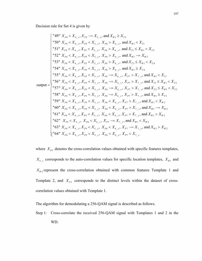
197
Decision rule for Set 4 is given by
4 4_ 5 5_ 1 5
4 4_ 5 5_ 6 6 _ 1 1
4 4 _ 5 5_ 6 6_ 1 1 2
4 4_ 5 5_ 6 6 _ 1 2
4
"49" , ~ , and
"50" , , , and
"51" , , , and
"52" , , , and ~
"53"
output
P x P x W T
P x P x P x W T
P x P x P x T W T
P x P x P x W W
P
X X X X X X
X X X X X X X X
X X X X X X X X X
X X X X X X X X
X X
< = ≥
< < > <
< < > ≤ <
< < > =
<
=
4_ 5 5_ 6 6_ 3 1 4
4 4_ 5 5_ 6 6 _ 1 4
4 4_ 5 5_ 6 6_ 7 7 _ 1 1
4 4_ 5 5_ 6 6_ 7 7 _ 1
, , , and
"54" , , , and
"55" , , ~ , , and
"56" , , ~ , , and
x P x P x T W T
P x P x P x W T
P x P x P x P x W T
P x P x P x P x T
X X X X X X X
X X X X X X X X
X X X X X X X X X X
X X X X X X X X X
< > ≤ <
< < > ≥
< < = > <
< < = > 1 2
4 4_ 5 5_ 6 6_ 7 7 _ 2 1 3
4 4_ 5 5_ 6 6_ 7 7 _ 1 3
4 4_ 5 5_ 6 6_ 7 7 _ 1 2
4 4_
"57" , , ~ , , and
"58" , , ~ , , and
"59" , , , , and
"60" ,
W T
P x P x P x P x T W T
P x P x P x P x W T
P x P x P x P x W W
P x
X X
X X X X X X X X X X X
X X X X X X X X X X
X X X X X X X X X X
X X
≤ <
< < = > ≤ <
< < = > ≥
< < < > <
< 5 5_ 6 6 _ 7 7 _ 1 2
4 4 _ 5 5_ 6 6_ 7 7 _ 1 2
5 5_ 6 6 _ 7 7 _ 1 2
4 4_ 5 5_ 6 6_ 7 7 _
, , , and ~
"61" , , , , and
"62" , , ~ , and
"63" , , , ~ , and
P x P x P x W W
P x P x P x P x W W
P x P x P x W W
P x P x P x P x
X X X X X X X X
X X X X X X X X X X
X X X X X X X X
X X X X X X X X
< < > =
< < < > >
< < = <
< < < = 1 2
4 4_ 5 5_ 6 6 _ 7 7 _"64" , , , W W
P x P x P x P x
X X
X X X X X X X X
⎧⎪⎪⎪⎪⎪⎪⎪⎪⎪⎪⎪⎪⎪⎨⎪⎪⎪⎪⎪⎪⎪⎪⎪⎪
>⎪⎪
< < < <⎪⎩
where #PX denotes the cross-correlation values obtained with specific features templates,
#_ xX corresponds to the auto-correlation values for specific location templates, 1WX and
2WX represent the cross-correlation obtained with common features Template 1 and
Template 2, and #TX corresponds to the distinct levels within the dataset of cross-
correlation values obtained with Template 1.
The algorithm for demodulating a 256-QAM signal is described as follows.
Step 1: Cross-correlate the received 256-QAM signal with Templates 1 and 2 in the
WD.
198
Step 2: Determine the quadrant location of each signal symbol and cross-correlate the
templates 1P , 2P , 3P , 4P , 5P , 6P and 7P with the received signal.
Step 3: Compute the auto-correlation of each of the templates 1P , 2P , 3P , 4P , 5P , 6P
and 7P .
Step 4: Compare the cross-correlation results from Step 1 with the thresholds as
described in the four sets of decision rules, and assign the appropriate indicator
for each signal segment.
Step 5: Recover the baseband data sequence based on the results obtained in Step 4.
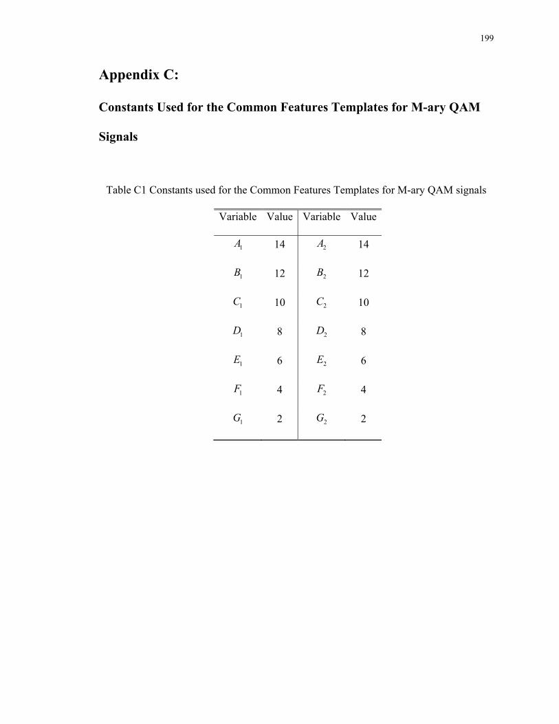
199
Appendix C:
Constants Used for the Common Features Templates for M-ary QAM
Signals
Table C1 Constants used for the Common Features Templates for M-ary QAM signals
Variable Value Variable Value
1A 14 2A 14
1B 12 2B 12
1C 10 2C 10
1D 8 2D 8
1E 6 2E 6
1F 4 2F 4
1G 2 2G 2

200
Curriculum Vitae
Ka Mun Ho
Education
May 2000 Bachelor of Science, Electrical and Computer Engineering Rutgers, the State University of New Jersey
May 2003 Master of Science, Electrical and Computer Engineering Rutgers, the State University of New Jersey
January 2010 Doctor of Philosophy, Electrical and Computer Engineering Rutgers, the State University of New Jersey
Employment 2004-2008 Summer Instructor
Department of Electrical and Computer Engineering Rutgers, the State University of New Jersey
2007-2008 Part-Time Lecturer Department of Mathematics Rutgers, the State University of New Jersey
2003-2007 Teaching Assistant Department of Electrical and Computer Engineering Rutgers, the State University of New Jersey
Publications 1. Ho, K. M., Vaz, C. and Daut, D. G., “Automatic Classification of Amplitude,
Frequency and Phase Shift Keyed Signals in the Wavelet-Domain,” 2010 IEEE Sarnoff Symposium, Princeton, NJ, USA, April 2010. (submitted for publication)
2. Ho, K. M., Vaz, C. and Daut, D. G., “A Wavelet-Based Method for Classification of Binary Digitally Modulated Signals,” 2009 IEEE Sarnoff Symposium, Princeton, NJ, USA, March 2009.
3. Ho, K. M., Vaz, C. and Daut, D. G., “Improved Demodulation of Phase Shift Keyed Signals Using Wavelet Thresholding,” 2008 IEEE Sarnoff Symposium, Princeton, NJ, USA, April 2008.
4. Ho, K. M., Vaz, K. and Caggiano, M., “ Scattering Parameter Characterization of Differential Four-Port Networks Using a Two-Port Network Analyzers,” Proc. 55th IEEE Electronic Components and Technology Conference, Florida, USA, May 2005.

201
5. Vaz, K., Ho, K. M. and Caggiano, M., “Error Reducing Techniques for the Scattering Parameter Characterization of Differential Networks Using a Two-Port Network Analyzer,” Proc. IEEE International Spring Seminar on Electronics Technology, Austria, May 2005.
6. Gazula I., Ho, K. M. and Caggiano, M., “Capacitance Extraction of Electronic Package Interconnects of Non-Parallel Configurations,” Proc. 11th International Symposium for Design and Technology of Electronic Packages, Romania, September 2004.
7. Caggiano, M. and Ho, K. M., “Electronics Packaging - A Course for the Rutgers University School of Electrical and Computer Engineering,” Proc. 54th IEEE Electronic Components and Technology Conference, Las Vegas, NV, USA, May 2004.
8. Zhang, W., Ho, K. M., Yeh, Y., Vaz, K. and Caggiano, M., “Circuit Modeling: Inductances and Resistances at Radio Frequencies,” Proc. 10th International Symposium for Design and Technology of Electronic Packages, Romania, September 2003.
9. Caggiano, M. and Ho, K. M., “Electronics Packaging - A Course for the Rutgers University School of Electrical and Computer Engineering,” Proc. 5th International Academic Conference on Electronic Packaging Education and Training, Dresden, Germany, March 2002.
10. Caggiano, M. and Ho, K. M., “Electronics Packaging - A CD-ROM Course for the Rutgers University School of Electrical and Computer Engineering,” Proc. 25th International Spring Seminar on Electronics Technology, Prague, Czech Republic, May 2002.
11. Ho, K. M., Rebelo, A. and Caggiano, M., “Electrical Modeling and Measuring Inductance in the Micro Lead Chip Carrier,” Proc. 52nd IEEE Electronic Components and Technology Conference, California, USA, May 2002, pp.1722-1728.
12. Caggiano, M. and Ho, K. M., “A Web-based Course for the IEEE Community,” Proc. 52nd IEEE Electronics Components and Technology Conference, California, USA, May 2002.
13. Caggiano, M. and Ho, K. M., “Electronics Packaging – A Course for the Rutgers University School of Electrical and Computer Engineering,” Proc. International Conference on Engineering Education, Manchester, UK, August 2002.