154 SNOW DEPTH RETRIEVAL USING KU-BAND INTERFEROMETRIC SYNTHETIC APERTURE RADAR (INSAR)

J.R. Evans a and F. A. Kruse b, c, *

a Department of Meteorology, b Physics Department, c Remote Sensing Center, Naval Postgraduate School, Monterey, CA USA 93943

Abstract Snow accumulation is a significant factor for hydrological planning, flood prediction, trafficability, avalanche control, and numerical weather/climatological modeling. Current snow depth measurement methods fall short of requirements. This research explored a new approach for determining snow depth using airborne interferometric synthetic aperture radar (InSAR). Digital elevation models (DEM) were produced using Multi-pass (monostatic) Single Look Complex (SLC) airborne Ku-band SAR for Snow-Off and Snow-On cases and differenced to determine elevation change from accumulated snow. A perturbation method that isolated and compared high frequency terrain phase to elevation was used to generate DEMs from the InSAR data. Manual snow depth measurements taken to validate the results indicated average InSAR snow depth errors of -8cm, 95cm, -49cm, 176cm, 87cm, and 42cm for six SAR pairs with respect to the measured ground truth. The source of these errors is not fully resolved, but appears to be mostly related to uncorrected slope and tilt in fitted low frequency planes. Results show that this technique has promise but accuracy could be substantially improved by the use of bistatic SAR systems, which would allow for more stable and measurable interferometric baselines. 1. INTRODUCTION

Monitoring seasonal snow accumulation is important as a factor required for evaluation of snow models, short- and long-term snow cover monitoring, and for both military and civilian operations. Improved spatial analysis of snow depth and volume can help decision makers plan for future events and mitigate risk. The use of remote sensing tools provides a way of covering large areas that are difficult to measure directly using other methods. The Naval Postgraduate School (NPS) is using Interferometric Synthetic Aperture Radar (InSAR) to explore snow depth estimation approaches. The Snow Depth Airborne Radar (SNODAR) project uses digital elevation models (DEMs) produced during “Snow-Off” and "Snow-On" conditions utilizing interferometric methods applied to airborne Ku-band Lynx SAR ________________________________________ * Corresponding author address: Fred A. Kruse, Physics Department, Naval Postgraduate School, 833 Dyer Rd, Monterey, CA 93943 USA; email: fakruse@nps.edu

data acquired on a General Atomics Aeronautical (GAA) King Air aircraft. Multi-pass (monotstatic) Single Look Complex (SLC) SAR data are spatially coregistered, SAR interferograms are produced to determine total wrapped phase, the wrapped interferograms are unwrapped, a flat earth correction is applied using a best-fit-plane perturbation model and a low-resolution DEM, and phase is converted to absolute height using linear regression to known elevations. Determination of the Snow-Off and Snow-On DEMs and subsequent subtraction provides an estimate of elevation change caused by snow accumulation for specific locations and an integrated snow volume over a specified area. Manual snow depth measurements and snow analysis were utilized to validate the SAR results in terms of snow depth, water content, and potential snow penetration. Participants in this research included the Naval Postgraduate School, Sandia National Laboratory, General Atomics Aeronautical, The Cold Regions Research and Engineering Laboratory US Army Research and Development Center (CRREL), and Mammoth Mountain California Ski Patrol. Cooperative research is also underway with the German Aerospace Center (DLR) utilizing their X-band SAR satellites (TerraSAR-X/Tandem-X). NPS is exploring future efforts utilizing a single-pass (bistatic) Ka-Band pass airborne system. The ultimate goal is to design operational approaches for regional snow depth determination using airborne and satellite SAR systems.

2. BACKGROUND

The requirement to measure snow depth over large areas is difficult to satisfy. The primary methods that have been used to-date for snow depth estimation include the Air Force Weather Agency’s Snow Depth and Sea Ice Analysis (SNODEP) model, the use of NASA’s SIR-C/X-SAR missions, the use of ground penetrating radar, and the use of LiDAR.

2.1 SNODEP The Air Force Weather Agency’s Snow Depth

and Sea Ice Analysis (SNODEP) model is the primary tool used today to provide military

operational users with snow depth information. Snow depth estimates are modeled using a combination of passive microwave imagery from the Special Sensor Microwave/Imager Sounder (SSM/IS) and surface observations to include synoptic, meteorological reporting observations (METAR) and Airways and snow depth climatology (AFWA, 2012a, 2012b).

SNODEP makes an initial snow depth estimate based on the previous model run, similar to the approach used in many numerical weather prediction models to establish an initial background field. Once the background field is established, the model incorporates any available surface snow depth observations. It uses an inverse linear weighting scheme to interpolate the data to the closest grid point. Then, in regions without surface reports, SSM/IS algorithms are used to detect snow. If no snow was previously detected, a value of 0.1m of snow depth is automatically assigned. If snow is detected where snow was previously detected, the snow depth estimate is trended toward climatology. If no snow is detected, the estimate for the area remains snow free.

The main strength of SNODEP is its ability to provide a global view of snow coverage. It does, however, have several weaknesses. Due to the inherent resolution of the SSM/IS satellite; SNODEP’s best resolution is 25km (Foster 2011). This spatial resolution typically is not adequate to provide the detail that operational users require. Its grid can also be too large to adequately estimate the snow depth in smaller watersheds, especially in complex terrain such as mountainous regions. In addition, the in-situ observations are extremely limited and the observations tend to be concentrated in more developed countries like the U.S. Many stations record snowfall, which should not be confused with snow depth on the ground. Mechanisms such as settling, melting, sublimation, and movement of snow by wind make the snowfall measurements a poor estimate of snow depth. Thus, inadequate characterization of spatial variability is a big concern. To make up for this poor coverage of in-situ observations the SSM/IS passive microwave satellite is used to determine the snow depth everywhere else. SSM/IS does this by using a correlation coefficient between the microwave brightness temperature and snow depth. This coefficient assumes snow crystal grain size, and that the snow is dry or refrozen. Failure of either of these assumptions can negatively affect the accuracy of the model. Furthermore, snow depth estimates from the SSM/IS are limited to depths of 40cm or less. The

snow depth algorithm becomes unreliable when the snow depth exceeds 40cm (Northrop Grumman 2010).

2.2 SIR-C/X-SAR The Spaceborne Imaging Radar-C/X-band

Synthetic Aperture Radar (SIR-C/X-SAR) flew two missions on NASA’s space shuttle in 1994, imaging 57.6 million square miles, or approximately 14 percent of the Earth’s surface (Stofan et al. 1995; JPL, 2012a, 2012b). The space shuttle launched with three different synthetic aperture radar (SAR) antennas. These included L-band (23.5cm wavelength), C-band (5.8cm wavelength), and X-band (3cm wavelength) antennas. The L and C bands were also capable of polarimetric measurements. The use of the three different bands allowed collection of information about the Earth’s surface at multiple scales, which had never been possible before with only single band SAR systems.

Snow characteristics have a large effect on the backscattering of radar emissions, thus a multifrequency, polarimetric SAR system has several advantages over other sensors for snow depth estimation. Parameters affecting what can be measured include (Shi and Dozier, 1996):

1. Sensor characteristics, to include

frequency/wavelength, polarization, and viewing angle

2. Snow pack parameters to include snow density, depth, particle size, size variation, liquid water content (stickiness), and stratification

3. Ground parameters to include dielectric and roughness parameters

Differences in backscattering properties by different radar wavelengths on the snow pack can be leveraged to determine the physical characteristics of the snow pack and the underlying ground. All three of the SIR-C/X-SAR wavelengths are assumed to penetrate into the snowpack. Based on electro-magnetic scattering theory, for a given material, there is a direct relationship between the wavelength and the depth of penetration (Richards, 2009). With that in mind, there should be an increase in backscattering moving from the L-band radar down to the X-band radar. This fact was used by Shi and Dozier (2000a, 2000b), to retrieve snowpack properties. They first used polarized data from the L-band radar to determine snowpack density. L-band proved to be a long enough wavelength that the backscatter from the

snowpack was negligible. The entire radar return therefore came from the ground below the snow pack. Despite the lack of backscatter from the snow, they were able to capitalize on the fact that the snow pack caused a shift in refraction in the incidence angle of the radar pulse. The extent of the refraction was dependent on the density of the snow pack. Furthermore, there was a difference in both the magnitude and relation between the VV and HH polarizations. By modeling this interaction, they were able to derive the snowpack’s density.

Due to the large variability in density in snowpacks, however, the density alone is not enough to estimate other characteristics of the snow pack such as snow depth or snow water equivalent (SWE). To do this Shi and Dozer (2000a, 2000b) used data from both the C-band and X-band radars. Both C-band and X-band radar pulses have different volume scattering properties. This fact was used to model the particle size and expected magnitude of the scattering. Both bands were assumed to penetrate to the ground in addition to the volume scattering, which added an additional component to the overall return. This was accounted for, however, by using the ground roughness and dielectric properties determined from the L-band radar.

This approach of using a combination of all three SAR bands showed very positive results and has stood up well to ground validation. While this technique has shown great potential, there are not, however currently any spaceborne or airborne sensors with the appropriate configuration to take advantage of this technique.

2.3 Ground Penetrating Radar There have also been attempts to use ground

penetrating radar (GPR) to address the issue of determining snow depth and other snowpack characteristics (Marshall et al., 2005). Frequency modulated continuous wave (FMCW) radar has proven to be the most successful of the GPRs for snow study. The FMCW radar works similarly to a standard radar system in that it times the pulse to determine range. It however uses a broad band width that results in a greater theoretical vertical resolution as compared to a standard GPR (Yankielun et al. 2004). This greater vertical resolution is quite important if you want to determine snow pack stratigraphy, which can be particularly important for avalanche prediction. Ground penetrating radars are typically deployed for snow pack analysis either by hand or by towing them behind a snowmobile. Recently they have

been deployed using low flying helicopters with some success (Marshal et al. 2008). Overall, the use of these FMCW radars has been quite successful at determining snowpack characteristics; in particular those characteristics that concern avalanche experts in focused areas. They are not, however, suited for covering larger areas. Deploying them on the ground, whether by hand or being towed behind a snowmobile or snowcat, does not provide nearly the spatial coverage provided by airborne systems. Ground deployment is also restricted by complex terrain. The use of the GPR by helicopter also has drawbacks. The systems used to-date have a fairly broad footprint. That means that as the GPR platform altitude increases, the area covered by the footprint also increases dramatically. Everything in the footprint is treated as a single return per pulse. The more the terrain varies within the footprint, the less reliable the measurements. Work done by Marshal et al. (2008) has shown that altitudes greater than 100ft above the ground make the data unreliable. Performance can be worse in areas where there are steep slopes. There are plans to try to use a FMCW GPR with a narrower beam to address this issue. With such restrictions, however, operational airborne collections in complex terrain are not currently possible.

2.4 LiDAR Light Detection and Ranging (LiDAR) is

another method that has been explored to estimate snow depth. LiDAR is based on measuring the time required for a pulse of light to travel to a target and then return to determine range (Hodgson et al. 2005). This can be used to build either 2-dimensional or 3-dimensional scenes. To determine snow depth, the scene is imaged with and without snow and then differenced, resulting in a snow volume and snow depth estimate at each specific point. The use of LiDAR has a lot of advantages. The first is that it can be used to cover large areas in an unobtrusive manner. It is also highly accurate, with accuracies down to the millimeter level in some cases (Osterhuber et al. 2008).

LiDAR has been deployed two different ways to determine snow depth. The most accurate way is to deploy the LiDAR system on the ground. Osterhuber et al. (2008) used a ground based unit that could either be placed on the ground or fixed to a surveyor’s tripod. In a snow pack with an average depth of just over two meters the LiDAR averaged a mean difference between manual and LiDAR measurements of 5.7 cm. While the use of

the ground-based system has potential, it also has some drawbacks. Systems currently being used are range-limited to about 1000 meters. Also, to generate a 3-D image, either multiple sensors are required, or the LiDAR has to be moved to different scanning locations. Furthermore, LiDAR becomes ineffective with any obscuring weather phenomena such as clouds, fog, or precipitation. This system may prove to be a great way of measuring snow depth at fixed locations but is not a good option for large regions of land or remote areas where a ground-based unit has not been placed.

The second way to deploy LiDAR is to operate the system from either an airborne or a spaceborne platform. Airborne LiDARs, also known as laser altimetry, are much better suited to cover large regions or remote areas than the fixed based systems (Hodgson et al. 2005). Airborne LiDAR depends on knowing the speed of light, the location of the laser emitter, and being able to time the laser pulse transmission to reception time. These data, like the ground based systems, can be used to generate a 3-D image or terrain model with a resolution at sub-meter level (Hopkinson et al. 2004). This has the same restriction as the ground based system in the fact that the laser path has to be free of visual obscurations. Accuracy also depends on the ability to position the aircraft to a high degree of x, y, z accuracy, which can potentially be problematic. Furthermore, there are a limited number of platforms that are currently equipped to perform this task.

2.5 InSAR DEM Subtraction The research summarized here is a first step

towards developing methods for determining snow depth utilizing InSAR technology. The approach is similar to LiDAR, however, snow depth is estimated by generating DEMs using SAR interferometry followed by subtraction of Snow-On from Snow-Off elevations. SAR has the advantage over LiDAR of being able to pass freely through most atmosphere conditions and through visible obscurations such as clouds and precipitation, allowing measurement of surface characteristics where optical wavelengths would be either absorbed or scattered. These obscurations are common during winter and can be a limiting factor for the use of laser-based systems for snow depth estimation.

From an operational standpoint, InSAR has another advantage. There are both current and planned satellite SAR systems that could be applied to the snow depth measurement problem, and numerous airborne platforms currently carry

SAR for other purposes, most notably the MQ-1 Predator and MQ-9 Reaper (General Atomic Aeronautical 2012). Many of these can potentially be adapted for operational InSAR snow depth determination beyond what is currently available using other methods.

Radar uses radiation emitted from an antenna in the microwave region of the electromagnetic (EM) spectrum. This emitted energy travels to a target and is then reflected back to the original, or in some cases an alternate antenna. The time it takes this radiation to travel the distance to and then back from the target is measured. Using the speed of electromagnetic propagation, this allows an estimate of the range to the target (Carrara et al. 1995). The wavelengths most commonly used in radar remote sensing are on the order of 1.5cm to 1m, or approximately 20GHz to 300MHz (Richards 2009). This frequency range is broken down into bands with L- (1–2 GHz), C- (4–8 GHz), and X-bands (8–12 GHz) as the most commonly used for remote sensing. This study used a slightly higher frequency Ku-Band (12–18 Ghz) radar.

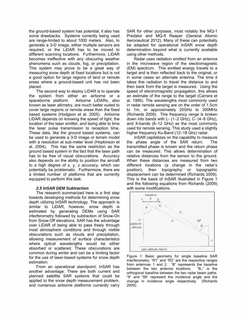
InSAR capitalizes on the capability to measure the phase angle of the SAR return. The transmitted phase is known and the return phase can be measured. This allows determination of relative distances from the sensor to the ground. When these distances are measured from two different locations (a change in the radar’s position), then topography or topographic displacement can be determined (Richards 2009). This is the basis of InSAR illustrated in Figure 1 and the following equations from Richards (2009) with some modifications.

Figure 1: Basic geometry for single baseline SAR interferometry. “R1” and “R2” are the respective ranges from antennas 1 and 2. “B” represents the baseline between the two antenna locations. “B┴” is the orthogonal baseline between the two radar beam paths. “θ” and “δθ” represent the incidence angle and the change in incidence angle respectively (Richards 2009).

The difference in the path lengths “R1” and “R2” in terms of the phase and a given baseline and incidence angle of “B” and “θ” respectively can be derived as:

θδθ sincos21 BRR += (1)

δθ is assumed to be approximately 0 using the plane wave approximation. The plane wave approximation considers the change in the incidence angle to approximate 0 when the target is infinitely far away when compared to the length of orthogonal baseline. This results in:

θsin21 BRR += (2)

Therefore

θsin21 BRRR =−=Δ (3)

The difference in phase angle “∆ϕ” associated with the change in path length “∆R” between the two passes can then be given as

λθπφ sin4 B=Δ

(4) (10)

This difference in phase angle is referred to as interferometric phase angle ∆ϕ. ∆ϕ can be obtained directly by simply imaging an area twice and taking the difference of the two recorded phases. The next step is to determine the relationship between the topographic height “h” and the incidence angle in order to get the phase to height ratio (Figure 2).

Figure 2: Determining the relationship between topographic height “h” and incidence angle “θ” with a platform altitude of “H” and range to the target of “R0” (Richards 2009).

From Figure 2, if “H” is the total height above an assumed altitude, and “R0” is the range to the target, observe that

θcos0RHh −= (5)

Taking the partial derivative of the topographic height with respect to the incidence angle results in

θθ

sin)(

0Rd

hd = (6)

Then taking the partial derivative of the interferometric phase angle ∆ϕ with respect to the incidence angle also results in

λθπ

θφ cos4)( B

d

d =Δ (7)

Combining equations (12) and (13) results in

θλθπθ

θφφ

sin

cos4

)(

)()(

0R

B

hd

d

d

d

dh

d =Δ=Δ (8)

We now have an expression for the change in interferometric phase with respect to the change in topographic height. Taking it one step further to make it more user friendly results in

θλθπ

θλπφ

sin)(

cos4

sin

4)(

0 hH

B

R

B

dh

d

−==Δ ⊥⊥

(9)

So as long as the incidence angle is known, the elevation above some known reference height (H-h) and the orthogonal baseline, the rate of change in elevation across an interferometric phase diagram per change of radian can be predicted. An interferometric phase factor αIF can be defined as

)( φα

Δ=

d

dhIF

(10)

and the height of a specific pixel will be given by

CONSTANTyxyxh IF +Δ= ),(),( φα (11)

Equation (11) enables the generation of a DEM from InSAR image pairs. The ability to use InSAR to generate DEMs is the basis for this research. High resolution InSAR DEMs generated during Snow-On conditions were subtracted from an InSAR Snow-Off DEM to estimate the snow depth utilizing airborne SAR.

APPROAThis r

approach determinaof laser athe snow acts to Taking thSnow-On snow deparea. Thground methods data for s

3.1 SiSelec

requiremerelatively relatively SAR resoGeneral Diego, Ccriterion orole in siteoptions duwinter seawere madultimately other loclocations only collec

Figure 3: (MammothAtomics ADiego, CA

ACH AND MEresearch usesimilar to th

ation of DEMsltimetry to macovered grouchange the he difference

and Snow-Opth and snowhis section svalidation used to extrnow depth de

ite Selectionction of thents for suff

obstacle freflat (i.e. no s

olution), accesAtomics fligh

CA. It shouof sufficient se selection. Tue to the lowason when thde. Mammot

met the reqcation. Eightwere identifiected for one s

Image-Map shh Mountain, CAAeronautical (G

(Google Earth

THODS ed airborne Sat taken for as. InSAR, waap both the bund. Snow c

elevation oe between thOff, allows dw volume ovummarizes tmeasuremenract DEMs fretermination.

n he study fficient snow ee, a clear steep slopesssibility, and bht radius celd be notedsnow depth pThere were n

w snow fall in he Snow-On h Mountain, quirements bt possible ded. SAR data site, “Elysian

howing locatioA) with respecGAA) home a, 2012).

SAR data in airborne LiDAas used insteare ground a

cover effectiveof the surfache two DEMetermination ver a specifihe study are

nts, and trom the InSA

site includdepth, beiview of sk

relative to tbeing within t

entered in Sd that the fiplayed a majnot many viab

the 2011-20measuremenCA (Figure

better than adata collectiwere ultimateFields”.

on of study arct to the Geneairfield near S

an AR ad nd ely ce. Ms,

of ed ea, he AR

ed ng ky, he he an rst jor ble 12 nts 3) ny on ely

rea eral San

3.2Cu

trihedrgroundSnow-provideand gcornereast-wElysian

ThSnow-to the emplacrecordlocatioof the Snow-the cometerswere pan elevcollect

Totechniqdepth On damade immeddisturbreflectoapproxoutlinemeasugrid. Tof the reflectomeasutaken area. tree-linfoliagemeasualong these dug coanalystempedensity

3.2Th

done ual. 199Atomicthe Ly

2 On-Site Grustom-designral reflectorsd locations in-On and Se ground con

geometric cor reflectors (west by 80m nn Fields site che first SAR -On condition

ground at eace the tripoded and a st

on. The stakereflectors to

-Off SAR collorner reflectos in snow depointed due svation angle tion parameteo ensure thatques’ accuracwas measure

ata collectionusing a 1cm

diately after thbed snow dors, the ximately eveed by the urements werThe in-situ snplanned analors to the

urements, rafurther sout These mea

ne to help pre on this murement locatwith calculatsnow depth m

oncurrently wsis near therature readiny measureme

2 SAR Data Che SAR data using a Lynx99) mounted cs Aeronauticynx system, a

round Controed field-po were depl the collectionow-Off SAntrol for radirrection of SCR) were p

north-south grcoordinates. data collect

ns, so the snoach corner reds. The GPtake was plae was critical o the same lolection. The ors varied beepth at this csouth or 167° of -13° to cor

ers and plannt the SAR sncy could be teed concurren. These mem graduated he data acqudirectly betwmeasuremenry 20 meterreflectors.

re taken in anow depth gridlysis area masouth. In andom meath of the plasurements erovide insightmethod. All tions were reted GPS erromeasuremen

with the SAR c northeast

ngs, crystal sents througho

Collection collection for

x II Ku-band to a King A

cal (GAA), thagreed to fly c

ol and Validaortable 25oyed at seln area during

AR collectionometric calibSAR data. laced on a rid centered o

was done dow was excaeflector locatPS locations aced to mar to allow for ocation durinsnow pits du

etween 1.5 tcollection sitemagnetic and

rrespond withed flight-lines

now depth retested, in-situ

ntly with the Seasurements avalanche

uisition. Due tween the cnts were rs within the

A total oa roughly 80d extended ouarked by the caddition to

asurements anned verificextended intt to the impa

the snow corded usingor. In additits, a snow pcollection for CR. It inc

size and typeout the column

r this researchradar (Tsunoir aircraft. Ge

he manufactucollection mis

ation dBsm lected g both ns to bration

Four 100m

on the

during avated ion to were

rk the return

ng the ug for to 2.3 e. CR d with

h SAR s. trieval snow

Snow-were

probe to the corner taken

e box of 16 0x80m utside corner these were

cation to the cts of depth

g GPS ion to it was snow

cluded e, and n.

h was oda et eneral urer of ssions

to generathis reseathat operawavelengof this sysresolution3.0m. Tathis study

Table 1: FOff SAR resolution. Snow-On a

The r

to includchange dpurposes made at the spotligcollections2012 respa flight levthe southlooking no

3.3 DD

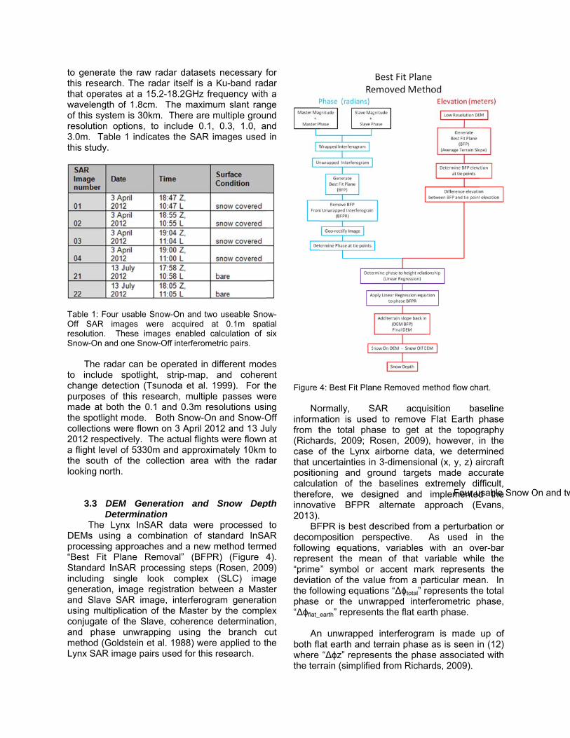
The DEMs usprocessin“Best Fit Standard including generatioand Slaveusing muconjugateand phasmethod (GLynx SAR

ate the raw raarch. The radates at a 15.2th of 1.8cm. stem is 30kmn options, to able 1 indicat.

our usable Snoimages were These imag

and one Snow-

radar can be de spotlight, etection (Tsuof this rese

both the 0.1 ght mode. Bs were flown pectively. Thevel of 5330mh of the collorth.

DEM GenerDeterminatio

Lynx InSARsing a combg approaches

Plane RemInSAR procesingle loo

n, image rege SAR imagltiplication of

e of the Slavese unwrappiGoldstein et aR image pairs

adar datasetsdar itself is a 2-18.2GHz fr The maxim. There are include 0.1,

es the SAR i

ow-On and twoe acquired ages enabled c-Off interferome

operated in dstrip-map,

unoda et al. 1arch, multipleand 0.3m re

Both Snow-Onon 3 April 20

e actual flight and approximection area

ration and on R data werebination of sts and a new

moval” (BFPRessing steps k complex

gistration betwe, interferogrthe Master b

e, coherenceing using thal. 1988) wereused for this

s necessary fKu-band rad

equency withum slant ranmultiple grou, 0.3, 1.0, aimages used

o useable Snoat 0.1m spatcalculation of etric pairs.

different modand cohere

1999). For te passes we

esolutions usin and Snow-O012 and 13 Juts were flown mately 10km with the rad

Snow Dep

e processedtandard InSAmethod termR) (Figure 4(Rosen, 200(SLC) ima

ween a Mastram generatiby the compl determinatio

he branch ce applied to tresearch.

for dar h a ge nd nd in

ow-tial six

es ent he

ere ng Off uly at to

dar

pth

to AR ed 4).

09) ge ter on ex

on, cut he

Figure 4

No

informafrom t(Richacase othat unpositiocalculatherefoinnova2013).

BFdecomfollowirepres“primedeviatithe follphase “∆ϕflat_e

An

both flawhere the ter

4: Best Fit Plan

ormally, Sation is usedthe total pha

ards, 2009; Rof the Lynx ncertainties inoning and gration of the ore, we desative BFPR

FPR is best dmposition per

ng equationsent the mea” symbol orion of the valowing equati

or the unwearth” represen

n unwrappedat earth and “∆ϕz” repres

rrain (simplifie

ne Removed m

SAR acqud to remove ase to get aRosen, 2009)airborne dat

n 3-dimensionround target

baselines esigned and

alternate a

described fromrspective. s, variables an of that vr accent malue from a paions “∆ϕtotal” r

wrapped internts the flat ea

interferograterrain phase

sents the phaed from Richa

Four u

method flow cha

isition basFlat Earth p

at the topog), however, ita, we determnal (x, y, z) ats made accextremely difimplemented

approach (E

m a perturbatAs used inwith an ove

variable whilrk representarticular mearepresents therferometric p

arth phase.

m is made e as is seen inse associated

ards, 2009).

usable Snow O

art.

seline phase

graphy in the mined

aircraft curate fficult, d the

Evans,

tion or n the er-bar e the ts the an. In e total phase,

up of n (12) d with

On and tw

totalφ =Δ From a phase is

eartflat _φΔ

The flat eno perturb

earthflat_φΔ

The terraiis

z φφ Δ=Δ

Unlike thethroughouaverage variation o

By replacphase can

Figure 5: Tphase. Thaverage slo

Figure 6: PUpper left Upper righof subtract

earthflatφ +Δ _

perturbation

eartflatth _φΔ=

earth phase, hbation. There

earthflath _φΔ=

in phase from

zz φφ ′Δ+

e flat earth ut the imagslope of theor perturbatio

cing (14) ann now be give

The Best Fit Plae BFPR isolateope of the terra

Path to the BFplane is a 3Dt plane is the bing the BFP fro

zφΔ+

perspective,

eartflatth _φ′Δ+

however, is aefore it reduce

h

m a perturbat

phase, therege. “∆ ” re terrain andon from that av

d (15) into en as

ane Removed (es the portion oain and is signi

PR. MammothD perspective vbest fit plane (Bom the total unw

(1

the flat ear

th (1

a plane and hes down to

(1

ion perspecti

(1

are variatiorepresents td “∆ ′” is tverage slope

(13), the to

(BFPR) methodof the total unwfied as “∆ϕz' ” o

h Mountain stuview of the SnBFP) generatewrapped phase

2)

rth

3)

as

4)

ve

5)

ns he he .

tal

totalφΔor

totalφΔ

Takingsame image

totalφΔ

Suphase totalφ −Δ

Equatiphase the BFterrainthe me

d subtracts thewrapped phase or the equivale

udy site, (37°37now-On unwrad from that intee. North is to th

earthflatl φΔ= _

earthflatl φΔ= _

g the best fit as finding thand is now g

earthflatl φΔ= _

ubtracting theyields

eflattotal φφ Δ=Δ− _

on (18) repspace) and

FP from the perturbation

ean slope (Fi

e best fit plane that is due to t

ent “δ∆ϕ”.

7.7’N, 119°02.7pped interferoerferogram, anhe top-center e

zzh φφ Δ+Δ+

zzh φφ Δ+Δ+

plane of the he average sgiven by

zth φΔ+

e BFP or (1

zzearth φφ −′Δ+Δ+

resents the demonstrate

total phase ns or terrain igures 5 and 6

(BFP) from thethe deviation o

7’N), Snow-Ongram, the tota

nd bottom centedge of the per

zφ′

zφ′

total phase slope of the p

17) from the

zearthflat φφ Δ−Δ− _

BFPR terraes that subtraresults in onthat deviates6).

e total unwrappof the terrain fro

n pairs 01/02 ral unwrapped pter plane is therspective views

(16)

is the phase

(17)

e total

zz φφ ′Δ=(18)

in (in acting ly the

s from

ped om the

esults. phase.

e result s.

Being ablunwrappefacilitates high frequremoves slope phSummarizgeneratiounwrappedeterminaresolutionknown gr

Figure 7: A(terrain slo119°02.7’N

Figure 8: Sstudy site, views.

le to generated interferogr

the isolationuency terrainthe flat eart

hase as szing (Figure n and remo

ed total phation of a BFPn DEM, differound contro

Adding the BFope in meters) N), Snow-On pa

Subtracting the (37°37.7’N, 11

te a best fit ram is importn of the phas. This approth phase anshown in e

4), the appoval of a Bhase imageP average sloerencing the l points and

PR after it hasresults in a D

airs 01/02 resu

Snow-Off DEM19°02.7’N), Sn

plane from ttant becausese produced oach effectived the averaequation (18

proach requirBFP from te (Figure 6ope from a lo

elevations correspondi

s had the lineaEM that is melts. North is to

M from the Snoow-On pairs 0

he e it by ely ge 8). res he 6); ow of

ng

elevaticalculaelevaticonveraddingand thSnow-estima(Figure

ar regression eeasured in metthe top-center

ow-On DEM res1/02 results. N

ions in theation and aion relation rt the BFPR g back in the en subtractin

-Off and Snated snow de 8).

equation applieters. Mammotedge of the pe

sults in a snowNorth is to the

e BFP DEapplication ousing a linephase imagelow resolutio

ng the DEMs now-On conddepths on a

ed to the low rth Mountain sterspective view

w depth image. top-center edg

M slope imof the phasear regressioe to elevationn slope (Figudetermined d

ditions to ga per-pixel

resolution DEMudy site, (37°3

ws.

Mammoth Moge of the persp

mage, se to on to n, and ure 7); during get to

basis

M BFP 37.7’N,

ountain pective

It is phase spto be of aaccurate eGPS at Mammoththe relaticomparingelevationsaverage resolutionthat the ptherefore,and elevabe appliedheight. Fielevationsimage. Tand elevaFigure 10entire BFresults interrain froRemovedAdding tcalculatedDEM resspatial res

Figure 9: Pand accomMountain simage pair

Figure 10: image pair and elevati

important toace and mus

any use in snoelevations recthe corner

h Mountain sion betweeng the meas at those slope as d

n (10m) DEMphase to elev a linear reg

ation results id to the entiregure 9 showss (CR) with rThe linear regation for thes0. ApplicatioFPR image a DEM bas

om the averag and Linethe BFPRL d mean slopults in a nesolution as th

Perspective viempanying elevstudy site, (37°.

Linear Regresshows the rela

ion.

o note that thst be convertow depth esticorded using reflector loc

site were use phase and

asured elevalocations re

determined M. Richards (vation relatio

gression betwn an equatioe scene to cos the locationrespect to thgression betwse four poin

on of the regon a pixel-

sed on pertuge slope “the earized” (BF

image to pe from the ew DEM at te SAR image

ew of BFPR wvations depict37.7’N, 119°02

sion for Snow ationship betwe

he BFPR is ted to elevatiimation. Higha survey gra

cations for ted to calculad elevationations to telative to tfrom the lo(2009) shownship is linea

ween the phan that can no

onvert to terrans of the knowhe 01/02 BFPween the phats is shown gression to t-by-pixel basurbation of t“Best Fit Pla

FPRL) imagthe previouslow resoluti

the same hie (Figure 7).

with CR tie pointed. Mammo2.7’N) 01/02 SA

On 01/02 SAReen the phase

in on hly de he

ate by he he ow ed ar, se ow ain wn PR se in

he sis he ne ge. sly on gh

nts oth AR

R

3. RE4.1 Sn

Snsix Snresultsduring SAR-daccurameasuboundeUnforturecordand ththe saThe elocatiometersaccurameasucalcularecord

Figure 1throughabove snthe 5m rthat localabeled (312 x 1

ESULTS ANDnow Depth Rnow depth wanow-On SA

s. Manual snthe field dep

determined snacy. As preurements weed by theunately, thosed with a stis meant that

ame as that estimated ac

ons was recors horizontal (acy limitationurements, anated for a raded locations

11: Manual snowout the scene annow depth imagradius area that wation. Corner ref(red outlined cir

176m), (37°37.7

D ANALYSISResults as calculatedR image p

now depth meployment wernow depths eviously desere measurede corner ree measuremtandard const the locationof the corneccuracy of rded to be on(x, y). Becaus imposed on average dius of five m(Figure 11).

w depth measurend are representege. The circle sizwas used to averflector locations rcles). Mammot’N, 119°02.7’N)

d utilizing a toairs with vaeasurements re compared to determine

scribed, the d on a 20meflector locaent locations

sumer-grade n accuracy waer reflector su

the snow n the order o

use of the locon the fieldsnow depth meters aroun

ements were takeed by the circles ze also demonstrrage the snow deare also shown

th Mountain stud), SAR pair 01/0

otal of arying taken to the

e their field

m grid ations. were GPS,

as not urvey. depth

of four cation snow

was nd the

en in the rates epth in and dy site 02.

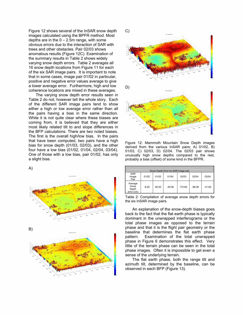
Figure 12 shows several of the InSAR snow depth images calculated using the BPFR method. Most depths are in the 0 – 2.5m range, with some obvious errors due to the interaction of SAR with trees and other obstacles. Pair 02/03 shows anomalous results (Figure 12C). Examination of the summary results in Table 2 shows widely varying snow depth errors. Table 2 averages all 16 snow depth locations from Figure 11 for each of the six SAR image pairs. It is important to note that in some cases, image pair 01/02 in particular, positive and negative error values average to give a lower average error. Furthermore, high and low coherence locations are mixed in these averages.

The varying snow depth error results seen in Table 2 do not, however tell the whole story. Each of the different SAR image pairs tend to show either a high or low average error rather than all the pairs having a bias in the same direction. While it is not quite clear where these biases are coming from, it is believed that they are either most likely related tilt to and slope differences in the BFP calculations. There are two noted biases. The first is the overall high/low bias. In the pairs that have been computed, two pairs have a high bias for snow depth (01/03, 02/03), and the other four have a low bias (01/02, 01/04, 02/04, 03/04). One of those with a low bias, pair 01/02, has only a slight bias. A)

B)

C)

D)

Figure 12: Mammoth Mountain Snow Depth images derived from the various InSAR pairs; A) 01/02, B) 01/03, C) 02/03, D) 02/04. The 02/03 pair shows unusually high snow depths compared to the rest, probably a bias (offset) of some kind in the BFPR.

Snow Depth Error by SAR image pair SAR

Image Pair

01/02 01/03 01/04 02/03 02/04 03/04

Average Snow Depth

error (cm)

-8.00 95.00 -49.06 175.69 -86.56 -41.69

Table 2: Compilation of average snow depth errors for the six InSAR image pairs.

An explanation of the snow-depth biases goes back to the fact that the flat earth phase is typically dominant in the unwrapped interferograms or the total phase images as opposed to the terrain phase and that it is the flight pair geometry or the baseline that determines the flat earth phase pattern. Examination of the total unwrapped phase in Figure 6 demonstrates this effect. Very little of the terrain phase can be seen in the total phase images. Often it is impossible to get even a sense of the underlying terrain.

The flat earth phase, both the range tilt and azimuth tilt, determined by the baseline, can be observed in each BFP (Figure 13).

Figure 13:depth erropairs and interferogra

For e(Figure 1north or ato that obtoward theFocusing to the hiindicate eastward average westwarderror. understoo

The coherenceat and thdistinct ddepth locato cohere14. The mat this timcausality; warrants f

Relationship or for each of

the pattern ofams.

example, for3), the range

away from thebservation, the east or the on the azim

igh and low a pattern wtilting azimuterror. Liktilting phas

The mechaod at this timesecond biase of the areae range phasifference betations and thnce. That ca

mechanism beme. The noted

however itfurther explor

between the nthe six interf

f the BFP der

r SAR Image phase tilts e radar platfohe azimuth pright side of tuth phase an

average erwhere the imth phase dem

kewise, for e there is anism behind

e. s noted invoa in the imagse tilt. Note tween the fi

he second eigan clearly be ehind this is d correlation t cannot beration.

normalized snoferometric imarived from tho

ge pair 01/up toward t

orm. In additiphase also tithe image arend comparingrrors seemsmages with monstrate a lo

those with a high averad this is n

olves both te being lookthat there is

rst eight snoght with respe

seen in Figunot understodoes not pro

e ignored a

ow age ose

02 he on ilts ea. g it

to an ow

a ge not

he ed

s a ow ect ure od ve nd

Figure with the

Th

have hthrougeight hbelow and somid-0.3coherebe absthis is returnscompato corrof the properradar observsolid gthere abe affshallowdecrearesponother p

14: Coherence field validatio

he first 8 snowhigh coherenchout the SAhave lower c0.7, with the

ome of the S3 range. Tence in some solutely deter

due to low vs at those parison againstroborate this. radar returnrties and the i

emission. ved to be sigground. In aare portions fected by aw incidence aase in the nsible for a depossibility is

e image for thon snow depth s

w depth measce, ranging ty

AR image pacoherence, tmajority betw

SAR image pThe exact re of the SAR irmined. It is values in theparticular loct the magnitu The strength

n is typicallyincidence angSnow radar

gnificantly lesaddition to thof the varyin

a shallow incangle could bmagnitude, ecrease in thea difference

he 01/02 InSAsample sites.

surement locaypically aboveairs. The setypically averween 0.5 andairs as low a

eason for themage pairs chowever likel

e magnitude ocations. A ude images sh of the magny due the sugle of the incor reflectivity ss than that oat, it appears

ng terrain thacidence ange responsibleand therefore coherence.in the liquid

AR pair

ations e 0.85 econd raging 0.65,

as the e low

cannot ly that of the quick

seems nitude urface oming

was of the s that t may

gle. A e for a re be One water

content ofrozen cocontent, tscenario facing slomelting thhours wharea has south throseen is ththere wasother wordgreater mweaker maway is ththe SAR second ei

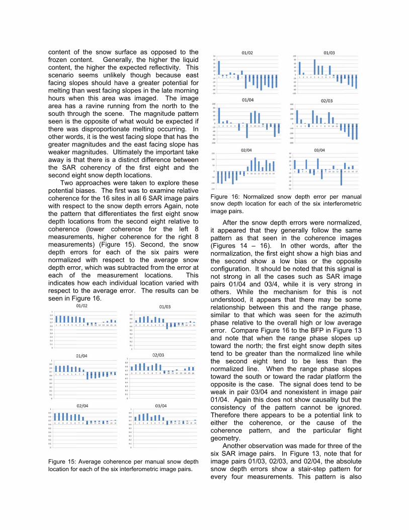
Two apotential bcoherencewith respethe patterdepth loccoherencemeasuremmeasuremdepth ernormalizedepth erroeach of indicates respect toseen in Fi

Figure 15: location for

of the snow ontent. Genhe higher theseems unlik

opes should hhan west facinhen this area

a ravine runough the scehe opposite os disproportiods, it is the w

magnitudes anmagnitudes. Uhat there is a

coherency ght snow depapproaches wbiases. The e for the 16 sect to the snorn that differeations from te (lower coments, higherments) (Figurrors for eac

ed with respor, which was

the measuhow each in

o the averageigure 16.

Average coher each of the si

surface as onerally, the he expected rekely though have a greatng slopes in tha was imagednning from thne. The ma

of what wouldonate melting

west facing slond the east faUltimately thea distinct diffeof the first

pth locations. were taken tofirst was to eites in all 6 SAow depth erroentiates the fthe second eoherence for coherence re 15). Secoch of the spect to the s subtracted frurement locdividual locate error. The

erence per max interferometr

opposed to tigher the liqueflectivity. Th

because eater potential fhe late mornid. The imahe north to tgnitude patte be expected

g occurring. ope that has tacing slope he important taerence betwe

eight and t

o explore thexamine relatiAR image paors Again, nofirst eight snoeight relative or the left

for the rightond, the snosix pairs weaverage snorom the error

cations. Thtion varied wresults can

nual snow depric image pairs

he uid his ast for ng ge he

ern d if

In he as ke en he

se ve irs

ote ow to 8

t 8 ow ere ow at

his with

be

pth .

Figure snow dimage p

Aftit appepattern(Figurenormathe seconfigunot strpairs 0othersundersrelationsimilarphase error. and notowardtend tothe senormatowardopposiweak i01/04. consisTherefeither coheregeome

Ansix SAimage snow every

16: Normalizedepth location pairs.

ter the snow eared that thn as that sees 14 – 16)lization, the fecond show uration. It shrong in all th01/04 and 0. While thestood, it appnship betweer to that whi

relative to thCompare Figote that whe

d the north; to be greater econd eight lized line. W

d the south oite is the casin pair 03/04 Again this d

tency of thefore there ap

the cohereence patternetry. nother observAR image pai

pairs 01/03, depth errorsfour measu

ed snow deptfor each of th

depth errorshey generallyeen in the c). In other first eight sho

a low biasould be noted

he cases suc03/4, while it e mechanismears that theen this and ich was seehe overall higgure 16 to theen the rangethe first eightthan the nortend to b

When the raor toward the se. The signa and nonexisdoes not showe pattern cappears to be ence, or thn, and the

vation was mairs. In Figure02/03, and 0 show a starements. Th

th error per mhe six interfero

s were normay follow the coherence im

words, afteow a high bias or the oppd that this sigch as SAR i

is very strom for this isere may be the range pn for the azgh or low ave BFP in Figu phase slopet snow depthrmalized line

be less thannge phase sradar platforal does tend stent in imagew causality bannot be ign

a potential lhe cause o particular

ade for three e 13, note th02/04, the absair-step patteis pattern is

manual ometric

alized, same

mages er the as and posite gnal is image ong in s not some

phase, zimuth verage ure 13 es up

h sites while

n the slopes m the to be

e pair ut the nored. ink to f the flight

of the hat for solute rn for

s also

similar in SAR image pair 01/02, but the signal is not as strong. Each of these stairsteps corresponds with one of the rows in which the snow depths were manually measured. The lower position numbers indicate measurements further north or further from the radar, and the higher position numbers are further south, or closer to the antenna. For example, the eastward row of four snow depths had the “1” position as the most northerly component. Each successive location went south through location “4” and started over again at position “5” at the top of the collection scene on the next row (Figure 14).

In each of these four cases the snow depth error decreases as the position moves south. This held true for every row regardless of whether there was a high or low bias. It also held true regardless of the amount of coherence. There are a couple of possibilities that could account for this. The first one is that there may be an error in the overall slope of the underlying Snow-Off DEM. Recall that the Snow-Off DEM is subtracted from the Snow-On DEMs. An error in the average slope of the Snow-Off DEM may account for this pattern. The same pattern is not, however, apparent in the other two scenes, which likely negates this line of reasoning. Another potential explanation is that the error is contained in the slope derived from the 10m DEM. Recall that the 10m DEM slope was added back into both the Snow-On and Snow-Off BFPRL images. If the slope has the wrong tilt it would be indicated as an increase in error in a particular direction. The weakness to that argument is that the same wrong slope is added to both the Snow-On and Snow-Off images. That should cancel the error out when those images are subtracted from each other. Another potential source lies with the BFP generated in the Snow-On images. It is assumed that average elevation slope for the Snow-On image is the same as that of the Snow-Off. This would be a good assumption if the snow laid evenly across the scene. We know that is not entirely true. The BFPR images from the Snow-On cases may actually have a different average terrain slope. After the Snow-On BFPR is linearized, it is added back in to the 10m DEM slope. It is assumed that the BFPRL image is a deviation from the average slope and that the Snow-On and Snow-Off images have the same average slope. If in fact they don’t, this will cause a regularly increasing error in a particular direction. For example, if the snow depth increases on average as one moves from the southern part of the image to the northern part of the image, the snow covered terrain slope will be steeper than that of the slope calculated from

the 10m DEM. This would mean that there would be error in the slope that is added back in.

5 SUMMARY AND CONCLUSIONS

The goal of the SNODAR Project research was to explore the viability of using Multi-pass Single Look Complex InSAR to determine snow depth. The SAR datasets were acquired by General Atomics using a Lynx II radar an airborne platform. Differencing of a Snow-Off DEM and Snow-On DEMs derived from intereferometric Ku airborne data using a perturbation or decomposition of parts approach was used to estimate snow depth.

We developed a method that removed the flat earth phase and mean slope contributions to the InSAR measurements by estimating a best fit plane for an unwrapped phase image combined with the average slope derived from a low-resolution DEM. The Best Fit Plane Removal (BFPR) method bypassed the requirement for detailed, precise InSAR baseline knowledge by using the perturbation or decomposition approach to isolate the interferometric phase caused by the terrain that deviated from the mean slope. It also removed the flat earth phase that can be difficult to determine without the baseline information. A linear regression was applied to the BFPR image to convert phase to terrain elevation, which was then added back to the average slope, resulting in a DEM at the 0.1m resolution of the InSAR data. After computing DEMs from both Snow-On and Snow-Off scenes they were differenced to calculate snow depth.

The snow depth results for six Snow-On SAR pairs were compared to 16 manually measured snow depth locations with varying degrees of success. The SAR image pairs showed an average error of -8cm, 95cm, -49cm, 175cm 87cm and 42cm for the respective six SAR pairs. The results also indicated that coherence of the unwrapped InSAR image played a role in the DEM generation. Of the 16 manually measured locations, eight fell in a high coherence regime indicated by coherences greater than 0.7 and the others fell in a regime indicated by coherence less than 0.7. In almost all of the cases the magnitude of the error for each of the SAR image pairs fell into two categories determined by these regimes.

There did appear to be a consistent pattern of either high or low bias in the BFPR-calculated snow depth results. Four of the SAR image pairs demonstrated a low average for the snow depths while the other two pairs demonstrated a high average. This pattern indicates that errors may be either related to or driven by the BFPs produced

from the unwrapped interferograms. There appear to be two different biases. The first is that the slope of the azimuth aspect of the BFP affects the direction of the bias. It was observed that an eastward tilt in the BFP was consistent with SAR pairs with a bias towards low snow depth errors. Those with a westward tilt demonstrated a bias towards high snow depth errors. The second bias is not as well defined, but appears to relate to coherence in the data and the range slope of the BFP. After normalizing the error there was a clear difference between the snow depth locations with high and low coherence. Additionally, the determination of whether the high or low coherence was above or below the normalization line appeared to be controlled by the range tilt of the BFP. This pattern is not fully understood. Furthermore, the observed pattern does not necessarily indicate causality. Additional SAR image pairs need to be tested to confirm the pattern.

Another observation was made in four of the six SAR image pairs. It appeared that regardless of the coherence, the calculated error decreased as the observations moved southward or in the direction toward the sensor. This is indicative of a possible issue in the slope of one or more of the BFPR elements. Slope issues could arise from the calculation of the BFP, accuracy of the low resolution DEM used to determine the deviation of the high frequency terrain from the average slope, or an issue with representativeness of the low resolution DEM relative to the true slope of the snow covered terrain.

This research demonstrates that Ku-band radar is capable of discerning the snow air interface with minimal penetration and of therefore mapping snow depth. This is evident in both its ability to see features on the snow surface such as tracks in the snow from the researchers, the high coherence obtained, and the representative DEMs extracted that consistently showed the terrain or snow surface. The DEMs also consistently showed the Snow-On terrain to be higher than that of the Snow-Off terrain.

6 RECOMMENDATIONS FOR FUTURE WORK

While perfect results were not achieved, the BFPR method shows promise. The foundation has been laid for further investigation. The greatest challenge in this research was achieving good DEMs utilizing multiple SAR passes with an aircraft with only one antenna and an unknown baseline. SAR acquisition using an aircraft equipped with a bistatic antenna system with a frequency in the Ku-band or higher would greatly

simplify the process and increase the probability of successful snow depth determination. While one of the main goals was to derive a method that could be used with operational monostatic platforms, it would benefit future research to test these techniques with a system that is better suited for DEM generation. The snow depth determinations would not then be dependent on the ability to derive DEMs using monostatic SAR platforms with the attendant baseline characterization problems. We are pursuing several research possibilities that use a bistatic InSAR approach. Once SAR interaction with the snow surfaces is better codified; the focus could transition to the operational platforms with only one antenna. These approaches should also be tested for a variety of snow conditions, as these affect radar returns from the surface and have the potential to affect the overall accuracy. Varying snow conditions from different times of the season with different properties should be explored to determine the effects on this technique. 7 ACKNOWLEDGEMENTS

We would like to thank Dr. Ralf Dunkel and the flight crews of General Atomic Aeronautical, who were instrumental obtaining the data used in this research. Without their support this project literally would not have been able to get off the ground.

Contributions made by Douglas Bickel at Sandia National Labs were also key to the success of this project. We would like to specifically acknowledge his input and guidance in developing mathematical approaches to the InSAR processing.

Alex Clayton of the Mammoth Mountain Ski Patrol played a critical role in determining the best location to conduct the research, helping to guide the on-mountain validation, and contributing extensively to on(in)-the-snow effort. Both Geoff Kruse and Maj. Paul Homan also spent many hours on the mountain digging holes and carrying equipment to the survey site. Without their efforts the research would not have been possible.

8 REFERENCES AFWA (Air Force Weather Agency) 2012a: AFWA

Algorithm Description Document (ADD) for the Air Force Weather Agency (AFWA) Snow Depth Analysis Model (SNODEP).

AFWA (Air Force Weather Agency), 2012b: AFWA Fact Sheet on Snow Depth and Sea Ice Analysis Model, [Available online at https://weather.afwa.af.mil/static/about_info/about_snow.html.].

Carrara, W. G., Goodman, R.S., Majewski R. M., 1995: Spotlight Synthetic Aperture Radar Signal

Processing Algorithms. 1st ed., Artech House, 554 pp.

Google Earth, “California.” Map. Google Maps. Web. Jun 2012: [Available online at http://www.google.com/earth/index.html.]

Evans, J. R., 2013, Determining Snow Depth using Airborne Multi-Pass Interferometric Synthetic Aperture Radar, Unpublished Ph.D. Dissertation, Naval Postgraduate School, Monterey, CA, 198 p.

Foster, J. L. et al., 2011: A blended global snow product using visible, passive microwave and scatterometer satellite data, International Journal of Remote Sensing, 32, 1371-1395

Goldstein R. M., Zebker H. A., and Werner C. L., 1988: Satellite radar interferometry: Two-dimensional phase unwrapping. Radio Science, 4, 713–720.

General Atomics Aeronautical, Sensor Systems, Lynx Multi-mode Radar, cited Dec 2012: [Available online at http://www.ga asi.com/products/sensor_systems/lynxsar.php.]

Hodgson, M. E., Jensen, J., Raber, G., Tullis, J., Davis, B. A., Thompson, G., Schuckman, K., 2005: An Evaluation of Lidar-derived Elevation and Terrain Slope in Leaf-Off Conditions. Photogrammetric Engineering & Remote Sensing, 71, 817–823.

Hopkinson, C., Sitar, M., Chasmer, L., and Treitz, P., 2004: Mapping Snowpack Depth beneath Forest Canopies Using Airborne LiDAR. Photogrammetric Engineering & Remote Sensing, 70, 323–330.

JPL (Jet Propulsion Laboratory), 2012a, SIR-C/X-SAR Flight Statistics, cited Aug 2012: [Available online at http://southport.jpl.nasa.gov/sir-c/getting_data/missions_stats.html.]

JPL (Jet Propulsion Laboratory), 2012b, What is SIR-C/X-SAR, cited Aug 2012: [Available online at http://southport.jpl.nasa.gov/desc/SIRCdesc.html.]

Marshall, H-P., Koh, G., and Foster, R. R., 2005: Estimating alpine snowpack properties using FMCW radar. Annals of Glaciology, 40, Issue 1, 157–162.

Marshall, H. P., Birkeland, K., Elder, K., and Meiners, T., 2008: Helicopter-Based Microwave Radar Measurements in Alpine Terrain. Proc. of the 2008 Int. Snow Science Workshop, Whistler, British Columbia, Canada, Telus Whistler Conference Center

Northrop Grumman, 2010: Algorithm and Data User Manual (ADUM) for the Special Sensor Microwave Imager/Sounder (SSMIS), Report-12621F CAGE/Facility Ident: 70143, 77 pp.

Osterhuber, R., Howle, J., and Bawden, G., 2008: Snow Measurement Using Ground-Based Tripod LiDAR. Western Snow Conference 2008. Hood River, OR.

Richards, J. A., 2009: Remote sensing with Imaging Radar. 1st ed. Springer-Verlag, 361 pp.

Rosen, P., 2009: InSAR Principles and Theory. UNAVCO Short Course Series- InSAR: An introduction to Processing and Applications for Geoscientists, Boulder, Colorado.

Shi, J. and Dozier J., 1996: Estimation of Snow Water Equivalence Using SIR-C/X-SAR. In IEEE, International Geoscience and Remote Sensing

Symposium, Remote Sensing for a Sustainable Future, 4, 2002–2004.

Shi, J. and Dozier J., 2000a: Estimation of Snow Water Equivalence Using SIR-C/X-SAR, Part I: Inferring Snow Density and Subsurface Properties. IEEE Transactions on Geoscience and Remote Sensing, 38, 2465–2474.

Shi, J. and Dozier J., 2000b: Estimation of Snow Water Equivalence Using SIR-C/X-SAR, Part II: Inferring Snow Depth and Particle Size. IEEE Transactions on Geoscience and Remote Sensing, 38, 2475–2488.

Stofan, E.R, et al., 1995: Overview of Results of Spaceborne Imaging Radar-C, X-Band Synthetic Aperture Radar (Sir-C/X-SAR). IEEE Transactions on Geoscience and Remote Sensing, 33, 817–828.

Tsunoda, S. I., Pace, F., Stence, J., Woodring, M., Hensely, W. H., Doerry, A. W., and Walker, B.C., 1999: Lynx: A high-resolution synthetic aperture radar. SPIE Aeroense, 3704, 1–8.

Yankielum, N., Rosenthal, W., and Davis, R.E., 2004: Alpine snow depth measurements from aerial FMCW radar. Cold Regions Science and Technology, 40, 123–134.