1210 est w yton da st. technical t repor uary janwahba/ftp1/boot.pdf1210 est w yton da st. madison,...
TRANSCRIPT

DEPARTMENT OF STATISTICSUniversity of Wisconsin1210 West Dayton St.Madison, WI 53706TECHNICAL REPORT NO. 913January 27, 1994
Bootstrap Con�dence Intervals for Smoothing Splines and theirComparison to Bayesian `Con�dence Intervals' 1byYuedong Wang and Grace Wahba
1Supported by the National Science Foundation under Grant DMS-9121003 and the National Eye Institute underGrant R01 EY09946. e-mail [email protected], [email protected]

Bootstrap Con�dence Intervals for Smoothing Splines and TheirComparison to Bayesian Con�dence IntervalsYuedong Wang and Grace Wahba yJanuary 27, 1994University of Wisconsin-MadisonUSAAbstractWe construct bootstrap con�dence intervals for smoothing spline and smoothing splineANOVA estimates based on Gaussian data, and penalized likelihood smoothing spline estimatesbased on data from exponential families. Several variations of bootstrap con�dence intervals areconsidered and compared. We �nd that the commonly used bootstrap percentile intervals areinferior to the T intervals and to intervals based on bootstrap estimation of mean squared er-rors. The best variations of the bootstrap con�dence intervals behave similar to the well knownBayesian con�dence intervals. These bootstrap con�dence intervals have an average coverageprobability across the function being estimated, as opposed to a pointwise property.Keywords: BAYESIAN CONFIDENCE INTERVALS, BOOTSTRAP CONFIDENCE IN-TERVALS, PENALIZED LOG LIKELIHOOD ESTIMATES, SMOOTHING SPLINES, SMOOTH-ING SPLINE ANOVA'S.1 IntroductionSmoothing splines and smoothing spline ANOVAs (SS ANOVAs) have been used successfully in abroad range of applications requiring exible nonparametric regression models. It is highly desirableto have interpretable con�dence intervals for these estimates for various reasons, for example, todecide whether a spline estimate is more suitable than a particular parametric regression. Aparametric regression model may be considered not suitable if a large portion of its estimate isoutside of the con�dence intervals of a smoothing spline estimate.One way to construct con�dence intervals for nonparametric estimates is via the bootstrap.Dikta (1990) constructs pointwise bootstrap con�dence intervals for a smoothed nearest neighborestimate. Hardle and Bowman (1988) and Hardle and Marron (1991) use bootstrap to constructpointwise and simultaneous con�dence intervals for a kernel estimate. Kooperberg, Stone andTruong (1993) construct bootstrap con�dence intervals for a regression spline estimate of a hazardfunction. Wahba (1990) suggests the use of an estimate-based bootstrap to construct con�denceintervals for a smoothing spline. Meier and Nychka (1993) used bootstrap con�dence intervals forspline estimates to obtain the properties of a statistic to test the equality of two rate equations. Asfar as we know, direct comparisons between smoothing spline bootstrap con�dence intervals andthe well known Bayesian con�dence intervals have not yet been done. In this paper, we providesome evidence that the bootstrap con�dence intervals for smoothing splines that we construct haveyAddress for correspondence: Department of Statistics, University of Wisconsin-Madison, 1210 West Dayton St.,Madison, Wisconsin 53706, USA. e-mail [email protected], [email protected]

an average coverage probability across the function being estimated (as opposed to a pointwiseproperty), similar to the Bayesian con�dence intervals. We also propose bootstrap con�denceintervals for SS ANOVAs and spline estimates for data from exponential families, which appearsto be new.The so-called Bayesian con�dence intervals were proposed by Wahba (1983) for a smoothingspline, where their frequentist properties were discussed. Gu and Wahba (1993b) extended Bayesiancon�dence intervals to the components of an SS ANOVA, and Gu (1992b) extended them to pe-nalized log likelihood smoothing spline estimates for data from exponential families. Wang (1994)extends the Bayesian con�dence intervals to a penalized log likelihood SS ANOVA estimate fordata from exponential families. It is well established that these Bayesian con�dence intervals havethe average coverage probability property, as opposed to a pointwise property (see Nychka (1988)).They have performed well in a number of simulations. See also Abramovich and Steinberg (1993),who generalize the Bayesian intervals to the case of a variable smoothing parameter. In this report,we compare the performance of bootstrap con�dence intervals with Bayesian con�dence intervalsvia simulations.In Section 2, we review Bayesian con�dence intervals and bootstrap con�dence intervals forsmoothing splines with Gaussian data. We show evidence supporting the average coverage prob-ability property of bootstrap con�dence intervals. Six variations of bootstrap con�dence intervalsare considered. We run several simulations to �nd the best bootstrap con�dence intervals andcompare them to Bayesian con�dence intervals. The parallel comparisons for SS ANOVA are givenin Section 3. In Section 4, we run a simulation to compare the performance of Bayesian con�denceintervals and bootstrap con�dence intervals for a penalized log likelihood smoothing spline estimatebased on binary data. We have found that the best variations of the bootstrap intervals behavesimilar to the Bayesian intervals. Bootstrap intervals have the advantage that they are easy toexplain and appear to work better than Bayesian intervals in small sample size experiments withGaussian data. The disadvantage of the bootstrap intervals is that they are computer intensive.2 Con�dence Intervals for Smoothing Splines2.1 Smoothing SplinesConsider the model yi = f(ti) + �i; i = 1; � � � ; n; ti 2 [0; 1]; (2.1)where � = (�1; � � � ; �n)T � N(0; �2In�n), �2 unknown and f 2 Wm whereWm = ff : f; f 0; � � � ; f (m�1) absolutely continuous, R 10 (f (m))2dt <1g. The smoothing spline f̂� isthe minimizer of 1n nXi=1(yi � f(ti))2 + � Z 10 (f (m)(t))2dt (2.2)over f 2 Wm. The smoothing parameter � controls the trade o� between the goodness of �t andthe roughness. When � is �xed, f̂� = (f̂�(t1); � � � ; f̂�(tn))T is a linear function of y = (y1; � � � ; yn)T :f̂� = A(�)y, where A(�) is the so called \hat" or in uence matrix. � can be selected by a data-based procedure such as generalized cross validation (GCV) or unbiased risk estimation (UBR) (seeWahba, 1990). The GCV estimate of � is the minimizer of the GCV functionV (�) = 1n jj(I � A(�))yjj2=[ 1ntr(I �A(�))]2:2

The UBR estimate of � is the minimizer ofU(�) = 1n jj(I �A(�))yjj2 + 2�2n trA(�);assuming that �2 is known. Denote �̂ as an estimate of � by one of these procedures. Denote f̂�̂as the solution of (2) with � = �̂.2.2 Bayesian Con�dence IntervalsSuppose that f in (2.1) is a sample path from the Gaussian processf(t) = mXj=1 �jtj�1(j � 1)! + b 12 Z t0 (t� s)m�1(m� 1)! dW (s);where W (�) is a standard Weiner process and � = (�1; � � � ; �m)T � N(0; �Im�m). Wahba (1978)showed that with b = �2n� ,f̂�(t) = lim�!1E(f(t)jy); �2A(�) = lim�!1Cov(f jy); (2.3)where f = (f(t1); � � � ; f(tn))T .This connection between a smoothing spline and the posterior mean and variance led Wahba(1983) to propose the (1� �)100% Bayesian con�dence intervals for ff(ti)gi=1;n asf̂�̂(ti)� z�2q�̂2[A(�̂)]ii; i = 1; � � � ; n; (2.4)where �̂2 = jjI � A(�̂)yjj2=tr(I � A(�̂)) is an estimate of �2. Both simulations (Wahba, 1983)and theory (Nychka (1988), Nychka (1990)) suggest that these Bayesian con�dence intervals havegood frequentist properties for f 2 Wm provided �̂ is a good estimate of the � which mini-mizes the predictive mean square error. The intervals must be interpreted \across the function",rather than pointwise. More precisely, Nychka de�nes the average coverage probability (ACP) as1nPni=1 P (f(ti) 2 C(�; ti)) for some (1� �)100% con�dence intervals fC(�; ti)gi=1;n. Rather thanconsider a con�dence interval for f(�), where f(�) is the realization of a stochastic process and� is �xed, he considers con�dence intervals for f(�n), where f is now a �xed function in Wmand �n is a point randomly selected from ftigi=1;n. Then ACP= P (f(�n) 2 C(�; �n)). DenoteTn(�) = 1nPni=1(f̂�(ti)� f(ti))2 as the average squared error. Let �0 be the value that minimizesETn(�). Let b(t) = Ef̂�0(t)�f(t) and v(t) = f̂�0(t)�Ef̂�0(t). They are the bias term and the varia-tion term of the estimate f̂�0(t) respectively. Set b = b(�n), v = v(�n) and U = (b+v)=(ETn(�0))1=2.Nychka argures that the distribution of U is close to a standard normal distribution since it is theconvolution of two random variables, one normal and the other with a variance that is small relativeto the normal component.We only consider ftigi=1;n as �xed design points. Let En be the empirical distribution forftigi=1;n. Assume supu2[0;1] jEn � uj = O( 1n).Assumption 1: �̂ is the minimizer of GCV function V (�) over the interval [�n;1), where �n �n�4m=5.Assumption 2: f is such that for some > 0, 1nPni=1(Ef�(ti)�f(ti))2 = �2(1+o(1)) uniformlyfor � 2 [�n;1). 3

Lemma 1 (Nychka) Suppose T̂n is a consistent estimator of ETn(�0). Let C(�; t) = f̂�̂(t) �z�2qT̂n. Then under Assumptions 1 and 2,1n nXi=1 P (f(ti) 2 C(�; ti))� P (jUj � z�2 ) �! 0uniformly in � as n �! 1.Nychka also proves (for m = 2) that�̂2trA(�̂)=nETn(�0) p�! 3227 as n �! 1: (2.5)So for large sample size, con�dence intervals with T̂n replaced by �̂2trA(�̂)=n should have ACPclose to or a little bit over the nominal coverage. Bayesian con�dence intervals actually use theindividual diagonal elements of A(�̂) instead of the average trA(�̂)=n. It is reasonable since mostof the diagonal elements are essentially the same (see Nychka (1988)).2.3 Bootstrap Con�dence IntervalsThe following bootstrap method is described in Wahba(1990). Suppose ftigi=1;n are �xed designpoints. Let f̂�̂ and �̂2 be the estimates of f and �2 from the data. Pretending that f̂�̂ is the \true"f , generate a bootstrap sample y�i = f̂�̂(ti) + ��i ; i = 1; � � � ; n;where �� = (��1; � � � ; ��n)T � N(0; �̂2In�n). Then �nd the smoothing spline estimate f̂ �̂�� basedon the bootstrap sample. Denote f�(ti) as the random variable of bootstrap �t at ti. Repeatthis process B times. So at each point ti, we have B bootstrap estimates of f̂�̂(ti). They are Brealizations of f�(ti). For each �xed ti, we will use six methods to construct a bootstrap con�denceinterval for f(ti):(A) Percentile-t interval (denoted by T-I). Similar to a Student's t statistic, consider Di = (f̂�̂(ti)�f(ti))=si, where si is an appropriate scale parameter. It is called a pivotal since it is independentof the nuisance parameter � in certain parametric models. We expect it to reduce the dependenceon � in our case. Denote D�i as the bootstrap estimate of Di, that is, D�i = (f �̂��(ti) � f̂�̂(ti))=s�i .Let x�2 , x1��2 be the lower and upper �=2 points of the empirical distribution of D�i . The (1 ��)100% T bootstrap con�dence interval is (f̂�̂(ti)� x1��2 si; f̂�̂(ti)� x�2 si): The standard deviationof f̂�̂(ti)� f(ti) generally equals a constant times �. So setting si = �̂, we have the T-I bootstrapcon�dence intervals.(B) Another percentile-t interval (denoted by T-II). From the Bayesian model, the exact standarddeviation of f̂�̂(ti)� f(ti) equals to q�̂2[A(�̂)]ii. Setting si = q�̂2[A(�̂)]ii in (A), we have the T-IIbootstrap con�dence intervals.(C) Normal interval (denoted by Nor). Let Ti = (f̂�̂(ti) � f(ti))2 be the squared error at ti.Denote T �i as the bootstrap estimate of Ti. The (1� �)100% normal bootstrap con�dence intervalis (f̂�̂(ti) + z�2 T �i ; f̂�̂(ti) + z1��2 T �i ); where z�2 , z1��2 are the �=2 and 1 � �=2 percentiles of thestandard normal distribution. We use the individual squared error estimate instead of averagesquared error because we want the length of a con�dence interval to depend on the distribution of4

the design points. Generally, the con�dence intervals are narrower in a neighborhood with moredata.(D) Percentile interval (denoted by Per) (Efron (1982)). Let f�L(ti), f�U (ti) be the lower and up-per �=2 points of the empirical distribution of f�(ti). The (1 � �)100% con�dence interval is(f�L(ti); f�U(ti)).(E) Pivotal method (denoted by Piv) (Efron (1981)). Let x�2 and x1��2 be the lower and upper�=2 points of the empirical distribution of f�(ti) � f̂�̂(ti). Then x�2 = f�L(ti) � f̂�̂(ti), x1��2 =f�U (ti) � f̂�̂(ti). If the empirical distribution of f�(ti) � f̂�̂(ti) approximates the distribution off̂�̂(ti) � f(ti), then P (x�2 < f̂�̂(ti) � f(ti) < x1��2 ) � 1 � �. The (1 � �)% pivotal con�denceinterval for f(ti) is (2f̂�̂(ti)� f�U (ti); 2f̂�̂(ti)� f�L(ti)).(F) Bias corrected percentile interval (denoted by BC) (Efron (1982)). Suppose there exists anincreasing function h such that� = h(f(ti)); �̂ = h(f�(ti)); �̂� = h(f�(ti)); �̂ � � � N(�a; 1); �̂� � �̂ � N(�a; 1);for some constant a. The (1 � �)100% biased corrected con�dence interval is (G��1n [�(2a +z�2 )]; G��1n [�(2a+z1��2 )]), where G�n is the empirical distribution of f�(ti), � is the density functionof a standard normal distribution, a = ��1(G�(f�(ti))).To study the properties of the bootstrap con�dence intervals, rewrite the expected averagesquared error as EfTn(�0) = 1n nXi=1Ef(f̂�0(tijf)� f(ti))2; (2.6)where f̂�0(�jf) is the smoothing spline estimate of f when f is the true function and the smoothingparameter is equal to �0. The bootstrap method replaces f by f̂�̂:EfTn(�0) � 1n nXi=1Ef̂�̂(f̂��0(tijf̂�̂)� f̂�̂(ti))2; (2.7)where f̂��0(�jf̂�̂) is the smoothing spline estimate of f̂�̂ when f̂�̂ is the true function. We can estimatethe right hand side of ( 2.7) since the true function f̂�̂ and true variance �̂2 are known. One way isto generate a bootstrap sample from this true model and �t a smoothing spline with �0 chosen byGCV or UBR. Repeat this procedure B times. The average squared error of these B repetitionscould be used as an estimate of the expected average squared error. The following theorem provesthat for �xed sample size such an estimation is consistent for the right hand side of ( 2.7). Forsimplicity of notation, we use f instead of f̂�̂ as the true function, �2 instead of �̂2 as the truevariance.Theorem 2 Suppose the true function f and variance �2 are known. Denote B bootstrap samplesas yj = f + �j ; j = 1; � � � ; B:Let f̂ j�0 be the smoothing spline �t for the jth bootstrap sample. Then for �xed n,1B BXj=1 1n nXi=1(f̂ j�0(ti)� f(ti))2 a:s:�! E 1n nXi=1(f̂�0(ti)� f(ti))2; B !1:5

[Proof] Write f̂�0 � f = (A(�0)� I)f +A(�0)�:Then 1n nXi=1(f̂�0(ti)� f(ti))2= 1n(f̂�0 � f)T (f̂�0 � f)= 1n [fT (A(�0)� I)2f + 2fT (A(�0)� I)A(�0)�+ �TA2(�0)�]:So E 1n nXi=1(f̂�0(ti)� f(ti))2 = 1n [fT (A(�0)� I)2f + �2trA2(�0)]:Similarly, we have1B BXj=1 1n nXi=1(f̂ j�0(ti)� f(ti))2= 1B BXj=1 1n [fT (A(�0)� I)2f + 2fT (A(�0)� I)A(�0)�j + (�j)TA2(�0)�j ]= 1nfT (A(�0)� I)2f + 2fT (A(�0)� I)A(�0) 1B BXj=1 �j + 1B BXj=1(�j)TA2(�0)�ja:s:�! 1nfT (A(�0)� I)2f + �2trA2(�0); B !1:So the bootstrap method tries to get an estimate T̂ �n of ETn(�0) directly. From Lemma 1,the bootstrap con�dence intervals C(�; t) = f̂�̂(t)� z�2qT̂ �n should have the ACP property ratherthan pointwise coverage. The normal intervals use individual squared error estimates at each datapoint instead of T̂ �n . They should have behave similar to the intervals using T̂ �n when the pointwisesquared errors are not too di�erent from each other. So we expect the normal bootstrap con�denceintervals to have the ACP Property, rather than a pointwise property. Actually all these bootstrapcon�dence intervals will be seen to have the ACP property from our simulations next.As pointed out by many authors, the bootstrap bias E(f̂ �̂��(t) � f̂�̂(t)jf̂�̂) generally underesti-mates the true bias E(f̂�̂(t) � f(t)jf), paticularly at bump points. Hall (1990) suggests using abootstrap resample of smaller size (say n1) than the original sample for kernel estimates. He showsthat for second-order kernels, the optimal choice of n1 is of order n1=2. It is hard to get a goodestimate of n1 in practice. Furthermore, a bootstrap sample of size n1 may give a very bad smooth-ing spline estimate. Dikta (1990) and Hardle and Marron (1991) suggest using an undersmoothedestimate to generate the bootstrap samples. They prove that after the right scaling, for a kernelestimate f̂�̂ with �̂ as the optimal bandwidth, f̂ �̂��(t)� f̂�̂1(t) and f̂�̂(t)�f(t) have the same limitingdistributions as n ! 1, if �̂1 tends to zero at a rate slower than �̂. Again, it is di�cult to getan estimate of �̂1 in practice. The optimal �̂1 depends on some order of derivative of f . Also,the performance for �nite samples may not be satisfactory, which is shown in their simulations.Here we do not intent to construct pointwise con�dence intervals. Instead, we only need a decentestimate of ET (�0). Without trying to estimate the bias, the bootstrap estimates of mean squarederror proved satisfactory in our simulations. 6

2.4 SimulationsIn this section, we use some simulations to(1) study the performance of 6 kinds of bootstrap con�dence intervals and �nd out which are better;(2) show the ACP property of bootstrap con�dence intervals;(3) compare the performance of bootstrap con�dence intervals with the Bayesian con�dence inter-vals.The experimental design is the same as in Wahba (1983). Three functions are used:Case 1 f(t) = 13�10;5(t) + 13�7;7(t) + 13�5;10(t);Case 2 f(t) = 610�30;17(t) + 410�3;11(t);Case 3 f(t) = 13�20;5(t) + 13�12;12(t) + 13�7;30(t);where �p;q(t) = �(p+q)�(p)�(q)tp�1(1� t)q�1; 0 � t � 1:n = 128 n = 64 n = 32Case 1 2 3 1 2 3 1 2 3� = .0125 0 0 0 0 4 4 8 70 100� = .025 0 0 0 0 3 4 7 24 57� = .05 0 0 0 0 3 4 7 12 22� = .1 0 0 0 0 0 2 7 8 11� = .2 0 0 0 0 0 0 7 7 8Table 2.1: Number of replications out of 100 total that have ratio �̂=� < 0:001.Case 1, Case 2 and Case 3 have 1, 2 and 3 bumps respectively (see plots next). They re ectan increasingly complex `truth'. The experiment consists of 3 � 3 � 5 = 45 combinations of Case1, 2, 3, n=32, 64, 128 and �=0.0125, 0.025, 0.05, 0.1 and 0.2. In all cases, ti = i=n. Data aregenerated for 100 replications of each of these 45 combinations. In all simulations in this report,random numbers are generated using the Fortran routines uni and rnor of the Core MathematicsLibrary (Cmlib) from the National Bureau of Standards. Spline �ts are calculated using RKPACK(see Gu (1989)). Percentiles of a standard normal distribution are calculated using the CDFLIB,developed by B. W. Brown and J. Lovato and available from statlib.We use GCV to select �̂ in all simulations in this section. It has been noted that for a smallsample size, there is a positive probability that GCV selects �̂ = 0, especially for small �2. Inpractice, if only � is known to within a few orders of magnitude, these extreme cases can bereadily identi�ed. The numbers of replications out of 100 simulation replications which have ratio�̂=� < 0:001 are listed in Table 2.1. Examination of the simulation output reveals that we willhave the same numbers if we count cases with ratios smaller than 0:1, that is, there are no caseswith ratio between 0:1 and 0:001. The number decreases as sample size increases, � increases orthe number of bumps decreases. All these cases have their �̂ smaller than �14 in log10 scale, whileothers have �̂ between �9 to �4 in log10 scale. We do not impose any limitation on the rangeof � since we do not want to assume any speci�c prior knowledge. Instead, we can easily identifythese \bad" (interpolation) cases if we know � within 3 orders of magnitude, which is generally7

n = 128 n = 64 n = 32Case 1 2 3 1 2 3 1 2 3� = .0125T-I .935 .925 .932 .949 .956 .956 .955 .832 |T-II .925 .918 .923 .933 .945 .962 .948 .829 |Nor .958 .946 .950 .950 .923 .947 .890 .664 |Per .940 .927 .930 .934 .914 .919 .888 .681 |Piv .924 .905 .913 .911 .887 .915 .857 .645 |BC .919 .897 .905 .898 .878 .878 .849 .645 |� = .025T-I .938 .927 .933 .957 .951 .954 .960 .886 .773T-II .929 .919 .925 .938 .939 .938 .945 .878 .768Nor .960 .949 .952 .953 .937 .932 .911 .765 .634Per .940 .924 .931 .940 .924 .924 .907 .774 .640Piv .930 .910 .916 .923 .904 .898 .878 .728 .615BC .923 .903 .909 .914 .896 .893 .865 .727 .606� = .05T-I .939 .929 .932 .955 .950 .948 .962 .940 .907T-II .928 .920 .924 .936 .936 .935 .945 .933 .902Nor .957 .949 .954 .956 .943 .938 .922 .856 .809Per .940 .923 .930 .939 .926 .924 .907 .857 .818Piv .932 .914 .918 .923 .905 .907 .893 .814 .766BC .923 .908 .909 .915 .901 .901 .884 .804 .762� = .1T-I .938 .932 .929 .955 .948 .948 .964 .958 .944T-II .926 .923 .923 .933 .931 .935 .948 .950 .936Nor .956 .952 .955 .954 .945 .939 .922 .899 .869Per .942 .924 .929 .940 .929 .921 .909 .893 .865Piv .932 .922 .919 .929 .913 .910 .900 .866 .840BC .922 .914 .915 .915 .900 .902 .895 .852 .827� = .2T-I .937 .935 .930 .948 .954 .950 .958 .965 .958T-II .928 .926 .925 .931 .938 .937 .922 .951 .946Nor .959 .954 .952 .947 .950 .942 .906 .918 .904Per .944 .923 .925 .931 .930 .921 .896 .902 .889Piv .930 .926 .920 .918 .917 .916 .885 .881 .874BC .921 .916 .912 .906 .907 .905 .881 .864 .864Table 2.2: Mean coverages of 95% bootstrap con�dence intervals.8

n = 128 n = 64 n = 32Case 1 2 3 1 2 3 1 2 3� = .0125T-I .050 .038 .038 .077 .070 .395 .123 .220 |T-II .052 .038 .039 .078 .072 .081 .124 .219 |Nor .039 .041 .040 .060 .086 .083 .150 .214 |Per .045 .043 .044 .065 .082 .089 .147 .214 |Piv .055 .050 .049 .096 .109 .084 .161 .201 |BC .058 .054 .054 .110 .110 .107 .160 .199 |� = .025T-I .051 .042 .039 .046 .072 .075 .097 .215 .275T-II .054 .042 .041 .054 .074 .077 .104 .214 .273Nor .041 .039 .039 .053 .072 .078 .130 .218 .251Per .048 .046 .047 .056 .071 .078 .128 .220 .253Piv .055 .051 .051 .075 .096 .098 .143 .216 .245BC .060 .056 .054 .079 .099 .101 .149 .217 .245� = .05T-I .051 .046 .044 .050 .071 .075 .087 .143 .189T-II .057 .047 .044 .060 .074 .077 .098 .145 .190Nor .044 .042 .040 .055 .066 .074 .122 .171 .193Per .051 .047 .049 .059 .066 .071 .125 .171 .188Piv .057 .056 .053 .078 .098 .098 .140 .182 .198BC .065 .058 .059 .082 .099 .100 .146 .178 .205� = .1T-I .058 .051 .050 .052 .074 .075 .088 .111 .142T-II .062 .051 .049 .066 .077 .077 .096 .114 .142Nor .047 .043 .042 .058 .063 .071 .124 .137 .169Per .055 .048 .055 .062 .066 .069 .125 .137 .167Piv .062 .054 .053 .080 .094 .095 .139 .149 .170BC .071 .056 .054 .091 .101 .100 .139 .160 .172� = .2T-I .064 .053 .053 .059 .048 .047 .091 .084 .099T-II .067 .054 .053 .072 .055 .052 .110 .091 .100Nor .047 .046 .046 .064 .058 .057 .133 .126 .127Per .059 .050 .060 .077 .060 .063 .136 .128 .125Piv .068 .057 .056 .088 .083 .073 .142 .146 .140BC .076 .062 .062 .094 .083 .080 .140 .151 .149Table 2.3: Standard deviations of coverages of 95% bootstrap con�dence intervals.9

n = 128 n = 64 n = 32Case 1 2 3 1 2 3 1 2 3� = .0125 .967 .956 .960 .955 .930 .924 .897 .669 |(.032) (.040) (.039) (.076) (.088) (.091) (.149) (.207) |� = 0.025 .966 .958 .961 .961 .944 .940 .917 .769 .640(.036) (.041) (.040) (.050) (.076) (.081) (.126) (.218) (.251)� = 0.05 .963 .959 .961 .956 .947 .943 .923 .858 .809(.039) (.044) (.041) (.055) (.076) (.077) (.113) (.170) (.193)� = 0.1 .962 .963 .963 .952 .948 .945 .920 .906 .878(.043) (.039) (.034) (.058) (.076) (.076) (.129) (.134) (.166)� = 0.2 .961 .962 .960 .938 .953 .947 .884 .919 .907(.048) (.041) (.039) (.073) (.059) (.053) (.152) (.128) (.130)Table 2.4: Mean coverage and their standard deviations (inside the parentheses) of 95% Bayesiancon�dence intervals.true in practice. After identifying the \bad" cases, one can re�t by choosing � in a limited range.For our simulations, we simply drop these cases since they stand for the failure of GCV instead ofthe con�dence intervals and they are \correctable". That is, all summary statistics of coveragesare based on the remaining cases. Actually, for � as small as :0125 or :025 here, the con�denceintervals are visually so close to the estimate that they are hard to see. Con�dence intervals areunlikely to be very interesting in these cases. We decided to include these cases since we want toknow when these con�dence intervals fail.For all bootstrap con�dence intervals, B=500. Similar to the above argument, there is a positiveprobability that the bootstrap sample �t selects an extreme �̂� = 0. Since we know the true functionand variance when bootstrapping, we certainly can identify these \bad" cases and should drop them.So these \bad" repetitions are dropped when we calculate the bootstrap con�dence intervals. Thisis not a limitation to bootstrap con�dence intervals, but rather a subtle point one needs to be carefulwhen constructing bootstrap con�dence intervals. Our results here and in Wahba and Wang (1993)suggest that this phenomena of \bad" cases will not be noticeable in practice for n much biggerthan 100.In each case, the number of data points at which the con�dence intervals cover the true values arerecorded. These numbers are then divided by the corresponding sample sizes to form the coveragepercentage of the intervals on the design points. Tables 2.2 and 2.3 list the mean coverages and thestandard deviations of the 95% bootstrap con�dence intervals. For almost all cases, T-I, T-II, Norand Per bootstrap con�dence intervals are better than Piv and BC bootstrap con�dence intervals.T-I intervals work better than T-II's. Nor intervals are a little bit better than Per intervals. T-Iintervals are better than Nor intervals in small sample size cases but this is reversed in large samplecases. The average coverages are much improved when the sample size increases from 32 to 64 andimproved a little bit when the sample size increases from 64 to 128.In the remainder of this section, when we mention bootstrap con�dence intervals we mean eitherT-I or Nor bootstrap con�dence intervals. To compare with the Bayesian con�dence intervals,we use the same data to construct Bayesian con�dence intervals. The mean coverages and theirstandard deviations of 95% con�dence intervals are listed in Table 2.4. Comparing Tables 2.2, 2.3and 2.4. we see that for n = 32, bootstrap con�dence intervals have better average coverages and10

n = 128 n = 64 n = 32MSE�/MSE �̂=� MSE�/MSE �̂=� MSE�/MSE �̂=�� = .0125Case 1 1.196(.434) .979(.072) 1.154(0.457) .944(.144) 1.018(.604) .841(.208)Case 2 .989(.288) .964(.086) .991(.415) .889(.168) .333(.245) .502(.194)Case 3 1.060(.284) .954(.085) .956(.395) .859(.162) | |� = .025Case 1 1.231(.502) .983(.071) 1.210(.502) .964(.121) 1.109(.645) .879(.195)Case 2 1.047(.351) .969(.084) 1.071(.425) .922(.153) .647(.237) .632(.483)Case 3 1.091(.316) .963(.084) 1.042(.404) .904(.154) .356(.306) .503(.231)� = .05Case 1 1.266(.587) .985(.071) 1.238(.547) .967(.120) 1.209(.747) .905(.185)Case 2 1.106(.417) .972(.084) 1.120(.456) .935(.149) .897(.612) .765(.227)Case 3 1.121(.355) .969(.084) 1.093(.433) .928(.152) .716(.478) .704(.243)� = .1Case 1 1.301(.687) .987(.070) 1.268(.588) .971(.119) 1.286(.891) .926(.184)Case 2 1.166(.473) .980(.071) 1.151(.482) .945(.144) 1.066(.677) .845(.204)Case 3 1.152(.388) .978(.072) 1.124(.470) .942(.148) .933(.549) .816(.235)� = .2Case 1 1.326(.735) .988(.070) 1.236(.636) .972(.118) 1.256(1.000) .936(.186)Case 2 1.203(.537) .983(.072) 1.182(.518) .960(.127) 1.149(.715) .886(.196)Case 3 1.167(.437) .982(.072) 1.158(.518) .964(.124) 1.023(.543) .892(.205)Table 2.5: Mean coverage and their standard deviations (inside the parentheses) of the ratios ofbootstrap MSE and true MSE and ratios of estimated � and true �.smaller standard deviations than the Bayesian intervals. For n = 64, bootstrap con�dence intervalsand Bayesian con�dence intervals are about the same. For n = 128, Bayesian con�dence intervalshave average coverages a little bit over the nominal value, while bootstrap con�dence intervals haveaverage coverage a little bit under the nominal value.For each repetition of the experiment, we calculate the true MSE, bootstrap estimate of MSE(denoted by MSE�) and the estimate of � (denoted by �̂). We then get the ratios: MSE�/MSEand �̂=�. The average ratios and their standard deviations are listed in Table 2.5. Notice that �̂underestimates � on average, which agrees with Carter and Eagleson (1992). Thus the bootstrapsamples have smaller variation than they should. This causes the average coverages of bootstrapcon�dence intervals to be a little bit smaller than the nominal value. On the other hand, un-derestimation of �̂2 does help the performance of Bayesian con�dence intervals since �̂2trA(�̂)=noverestimates ETn(�0) (in theory) by a factor of 32=27. Carter and Eagleson (1992), who studiedthe same examples used here, found that for these functions, a better choice for the estimation of�2 is yT (I �A(�̂))2y=tr[I �A(�̂)]2. We don't know to what extent these results concerning �̂2 areexample-dependent, but we would expect that such a choice of �̂2 would make bootstrap con�denceintervals work better relative to the Bayesian intervals in the present experiments. Notice also thateven though the bootstrap bias is generally smaller than true bias, MSE� overestimates MSE onaverage, especially for large sample sizes. The variances of MSE�/MSE's are quite big.We visually inspect many of the plotted intervals and pointwise coverages. They all give a11

similar visual impression. Therefore, we just plot some \typical" cases. In Figure 2.1, we plotboth bootstrap con�dence intervals and Bayesian con�dence intervals when � = 0:2 for someselected functions and sample sizes. These cases are actually the �rst replicates in simulations.The pointwise coverages are plotted in Figures 2.2 and 2.3. It is obvious that the pointwisecoverages of bootstrap con�dence intervals are similar to Bayesian con�dence intervals'. That is,the pointwise coverage is smaller than the nominal value at high curvature points, particularly forPer intervals. These plots support the argument that the bootstrap con�dence intervals have theACP property.3 Component-Wise Con�dence Intervals for SS-ANOVA3.1 SS ANOVAsConsider the model yi = f(t1(i); � � � ; td(i)) + �i; i = 1; � � � ; n; ti 2 [0; 1]; (3.1)where � = (�1; � � � ; �n)T � N(0; �2In�n), �2 unknown, and tk 2 T (k), where T (k) is a measurablespace, k = 1; � � � ; d. Denote T = T (1) � � � T (d). Assume that f is in some reproducingkernel Hilbert space (RKHS) H (see Aronszajn (1950)). Suppose that H admits an ANOVA-likedecomposition (see Gu and Wahba (1993a) for details):H = [1]�Xk H(k) �Xk<l[H(k) H(l)]� � � � ; (3.2)here, [1] denotes the constant functions on T , and H(k) consists of functions depending only ontk , H(k) H(l) consists of functions depending on tk and tl, and so forth. An element fk in H(k)is called a main e�ect, an element fkl in H(k) H(l) is called a two factor interaction, and so on.Each H(k) can be further decomposed: H(k) = H(k)� � H(k)s , where H(k)� is �nite dimensional (the\parametric" part which is not penalized; usually polynomials), and H(k)s (the \smooth" part) isthe orthocomplement of H(k)� in H(k). After deciding on a model (that is, choosing which termsin ( 3.2) to retain, replacing H(k), H(l) and so forth in ( 3.2) by their decompositions, multiplyingout and regrouping, we can write the model space as M = H0 �Ppj=1Hj , where H0 is a �nitedimensional space containing functions which are not penalized, and the Hj are orthogonal. Theestimate f� of f is obtained by minimizing1n nXi=1(yi � f(t(i)))2 + � pXj=1 ��1j kP jfk2 (3.3)in M, where t(i) = (t1(i); � � � ; td(i)). P j is the orthogonal projection in M onto Hj . kP jfk2 is aquadratic roughness penalty. � is the main smoothing parameter, the �'s are subsidiary smoothingparameters, satisfying an appropriate constraint for identi�ability (see Wahba (1990), Gu andWahba (1993b)). This minimization also gives component-wise estimates such as main e�ects andtwo factor interactions. We would like to to construct con�dence intervals not only for the overallfunction f , but also for all components in the model. These con�dence intervals may, for example,be used as an aid in eliminating unimportant components, or deciding whether certain features are\real". 12

x
f(t)
0.0 0.2 0.4 0.6 0.8 1.0
-0.5
0.5
1.0
1.5
2.0
Case 1, n=32
x
f(t)
0.0 0.2 0.4 0.6 0.8 1.0
-0.5
0.5
1.0
1.5
2.0
Case 1, n=32
x
f(t)
0.0 0.2 0.4 0.6 0.8 1.0
01
23
Case 2, n=64
x
f(t)
0.0 0.2 0.4 0.6 0.8 1.0
01
23
Case 2, n=64
x
f(t)
0.0 0.2 0.4 0.6 0.8 1.0
-0.5
0.5
1.5
2.5
Case 3, n=128
T-I bootstrap intervalsx
f(t)
0.0 0.2 0.4 0.6 0.8 1.0
-0.5
0.5
1.5
2.5
Case 3, n=128
Bayesian intervalsFigure 2.1: Display of the 95% con�dence intervals for � = 0:2. Solid lines: true function; dottedlines: con�dence intervals. Top row: Case 1 and n=32; middle row: Case 2 and n=64; bottom row:Case 3 and n=128. Left column: T-I bootstrap intervals; right column: Bayesian intervals.13

******
************
**************************************
***************************************
*********************************
x
poin
twis
e co
vera
ge
0.0 0.2 0.4 0.6 0.8 1.0
0.0
0.2
0.4
0.6
0.8
1.0
Case 1, n=128
***************
***************************************
*****************************************
*********************************
x
poin
twis
e co
vera
ge
0.0 0.2 0.4 0.6 0.8 1.0
0.0
0.2
0.4
0.6
0.8
1.0
Case 1, n=128
***********
****************
****************
*****************************
**************************************
******************
x
poin
twis
e co
vera
ge
0.0 0.2 0.4 0.6 0.8 1.0
0.0
0.2
0.4
0.6
0.8
1.0
Case 2, n=128
*************************************************************************
*************************
******************************
x
poin
twis
e co
vera
ge
0.0 0.2 0.4 0.6 0.8 1.0
0.0
0.2
0.4
0.6
0.8
1.0
Case 2, n=128
****************
*****************
************
**********************
***********************
***************************
***********
x
poin
twis
e co
vera
ge
0.0 0.2 0.4 0.6 0.8 1.0
0.0
0.2
0.4
0.6
0.8
1.0
Case 3, n=128
T-I bootstrap intervals
***********************
***********************************
*********************************************************
*************
x
poin
twis
e co
vera
ge
0.0 0.2 0.4 0.6 0.8 1.0
0.0
0.2
0.4
0.6
0.8
1.0
Case 3, n=128
Bayesian intervalsFigure 2.2: Stars are pointwise coverage of 95% con�dence intervals when � = 0:1 and n=128.Dashed curves are the magnitude of j �f j. Left column: T-I bootstrap intervals; right column:Bayesian intervals. Top row: Case 1; middle row: Case 2; bottom row: Case 3.14

***************
***********************************
*********************************************
*********************************
x
poin
twis
e co
vera
ge
0.0 0.2 0.4 0.6 0.8 1.0
0.0
0.2
0.4
0.6
0.8
1.0
Case 1, n=128
************
****************************
************************************
******************************************
*******
***
x
poin
twis
e co
vera
ge
0.0 0.2 0.4 0.6 0.8 1.0
0.0
0.2
0.4
0.6
0.8
1.0
Case 1, n=128
***************
******************************************************************
********************
***************************
x
poin
twis
e co
vera
ge
0.0 0.2 0.4 0.6 0.8 1.0
0.0
0.2
0.4
0.6
0.8
1.0
Case 2, n=128
******
*****************************************************************
*********
****
*************
********************
***********
x
poin
twis
e co
vera
ge
0.0 0.2 0.4 0.6 0.8 1.0
0.0
0.2
0.4
0.6
0.8
1.0
Case 2, n=128
******
*****************
*******************************
********************************************************
***************
***
x
poin
twis
e co
vera
ge
0.0 0.2 0.4 0.6 0.8 1.0
0.0
0.2
0.4
0.6
0.8
1.0
Case 3, n=128
Nor bootstrap intervals
************
****
****************************
***********************************************************************
********
*****
x
poin
twis
e co
vera
ge
0.0 0.2 0.4 0.6 0.8 1.0
0.0
0.2
0.4
0.6
0.8
1.0
Case 3, n=128
Per bootstrap intervalsFigure 2.3: Stars are pointwise coverage of 95% con�dence intervals when � = 0:1 and n=128.Dashed curves are the magnitude of j �f j. Left column: Nor bootstrap intervals; right column: Perbootstrap intervals. Top row: Case 1; middle row: Case 2; bottom row: Case 3.15

3.2 Bayesian Con�dence Intervals for ComponentsSuppose that f in ( 3.1) is a sample path from the Gaussian processf(t) = MXk=1 �k�k(t) + b 12 pXj=1q�jZj(t)where � = (�1; � � � ; �m)T � N(0; �Im�m), M = dim(H0), �1; � � � ; �M span H0, the Zj 's areindependent, zero mean Gaussian stochastic processes, independent of � , with EZj(s)Zj(t) =Rj(s; t), where Rj(s; t) is the reproducing kernel of Hj . Gu and Wahba (1993b) show that withb = �2n� , f̂�(t) = lim�!1 E(f(t)jy), and that this relation holds with f̂� and f replaced by P j f̂�and P jf . They also get the posterior variances for each component. Then they construct Bayesiancon�dence intervals for each component similar to the univariate case.3.3 Bootstrap Con�dence Intervals for ComponentsSimilar to the univariate smoothing spline case, a component-wise bootstrap tries to estimate thedistribution of an SS ANOVA estimate directly. Following the same procedure as in the univariatecase, we �rst get estimates of f , components of f and �2. Then we generate a bootstrap sampleand �t with an SS ANOVA model f̂ �̂�� and collect its components. Repeat this process B times.Treating each component as a single function, we can calculate bootstrap con�dence intervals foreach component as in the univariate case. We construct T-I (simply denoted as T), Nor, Per, Pivand BC intervals in this case. We do not construct T-II intervals since they are inferior to T-I's.3.4 SimulationsWe use the same example function and the same model space as in Gu and Wahba (1993b).Let T = T (1) T (2) T (3) = [0; 1]3, f(t) = C + f1(t1) + f2(t2) + f12(t1; t2), where C = 5,f1(t1) = e3t1 � (e3 � 1)=3, f2(t2) = 106[t112 (1 � t2)6 � �12;7(t2)] + 104[t32(1� t2)10 � �4;11(t2)], andf12(t1; t2) = 5 cos(2�(t1 � t2)), where �p;q is the Beta function. We �t with a model having threemain e�ects and one two factor interaction: f(t) = C + f1(t1) + f2(t2) + f12(t1; t2) + f3(t3).We only run simulations for n=100 (n=200 is too computer intensive) with three levels of � (1,3 and 10). GCV method is used to choose smoothing parameters for all simulations. B=100 forall simulations. 100 replicates are generated for each experiment, and data for the 95% con�denceintervals are collected. In each case, the number of data points at which the con�dence intervalscover the true values of f , f1, f2, f12 and f3 are recored. These numbers are then divided bythe sample size to form the coverage percentage of the intervals on design points. We summarizethese coverage percentages using box-plots (Figures 3.1, 3.2 and 3.3). We only plot the box-plotsfor T, Nor, Per and Piv intervals since they are uniformly better than BC intervals. Similar tothe smoothing spline case, the GCV criterion selects �̂ � 0 (nearly interpolates the data) in oneof the one hundred � = 1 replicates, in one of the � = 3 replicates and in two of the � = 10replicates. Again, these cases can be readily detected by examining estimates of �2 which areorders of magnitude smaller than the true values. We exclude these four cases.From these box-plots, we see that T, Nor, Per and Piv intervals work well. T and Nor intervalsare a little bit better than Per and Piv intervals. The good performance of Nor intervals suggeststhat Lemma 1 might be true for component-wise Nor intervals. Comparing with the box-plots ofGu and Wahba (1993b) in the top row of their Figure 1, we can see that T bootstrap con�denceintervals have somewhat better mean coverages and smaller variability than the Bayesian con�dence16

0.0
0.4
0.8
*****
********
*
***
*
**********
f f f f f 1 2 12 3
Ave
rage
Cov
erag
e
T
+ + + + +
0.0
0.4
0.8
*
****
*
***********
****
*
*****************
f f f f f 1 2 12 3A
vera
ge C
over
age
Nor
+ + + + +
0.0
0.4
0.8
*
***
*
***********
**
*
*************
f f f f f 1 2 12 3
Ave
rage
Cov
erag
e
Per
+ + ++ +
0.0
0.4
0.8
*
*
*
*
****
*
***
********
f f f f f 1 2 12 3
Ave
rage
Cov
erag
e
Piv
+ + + + +
Figure 3.1: Coverage percentages of 95% bootstrap intervals when � = 1, for T, Nor, Per and Pivmethods. Plusses: sample means; dotted lines: nominal coverage.17

0.0
0.4
0.8
*
********
* ***************
f f f f f 1 2 12 3
Ave
rage
Cov
erag
e
T
+ + + + +
0.0
0.4
0.8
***** ***
*****
***
**
**
*********
f f f f f 1 2 12 3A
vera
ge C
over
age
Nor
+ + + + +
0.0
0.4
0.8
*
*
***
* ***
*
************
f f f f f 1 2 12 3
Ave
rage
Cov
erag
e
Per
+ + + + +
0.0
0.4
0.8
*
***
***
** *
**********
f f f f f 1 2 12 3
Ave
rage
Cov
erag
e
Piv
+ + + + +
Figure 3.2: Coverage percentages of 95% bootstrap intervals when � = 3, for T, Nor, Per and Pivmethods. Plusses: sample means; dotted lines: nominal coverage.18

0.0
0.4
0.8
**
******* *
******************
f f f f f 1 2 12 3
Ave
rage
Cov
erag
e
T
+ ++
++
0.0
0.4
0.8
****
**************
**
********
f f f f f 1 2 12 3A
vera
ge C
over
age
Nor
+ ++
++
0.0
0.4
0.8
*****
****
****
*** *
*******
f f f f f 1 2 12 3
Ave
rage
Cov
erag
e
Per
+ ++
++
0.0
0.4
0.8
*
**
*****************
f f f f f 1 2 12 3
Ave
rage
Cov
erag
e
Piv
+ ++
++
Figure 3.3: Coverage percentages of 95% bootstrap intervals when � = 10, for T, Nor, Per and Pivmethods. Plusses: sample means; dotted lines: nominal coverage.19
0.0 0.2 0.4 0.6 0.8 1.0
-10
-50
510
x1
f 1
0.0 0.2 0.4 0.6 0.8 1.0
-10
-50
510
x2
f 2
T intervals for main effects
0.0 0.2 0.4 0.6 0.8 1.0
-10
-50
510
x3
f 3
0.0 0.2 0.4 0.6 0.8 1.0
-10
-50
510
x1
f 1
0.0 0.2 0.4 0.6 0.8 1.0
-10
-50
510
x2
f 2
Nor intervals for main effects
0.0 0.2 0.4 0.6 0.8 1.0
-10
-50
510
x3
f 3
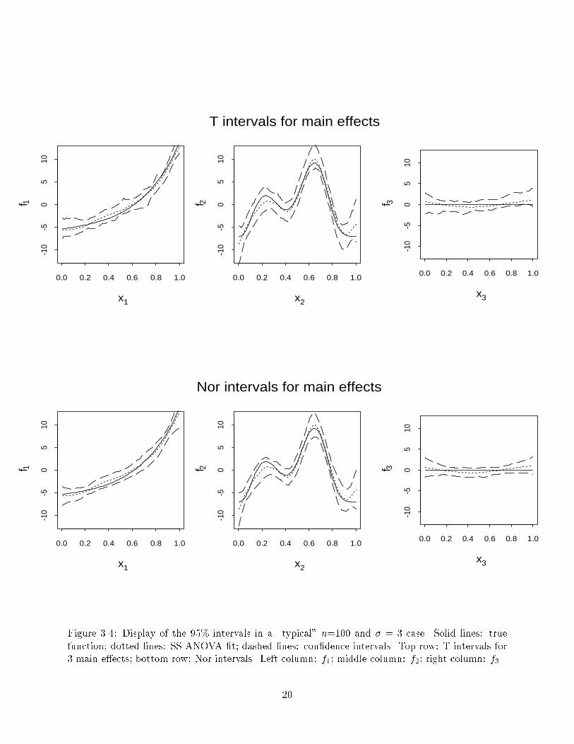
Figure 3.4: Display of the 95% intervals in a \typical" n=100 and � = 3 case. Solid lines: truefunction; dotted lines: SS ANOVA �t; dashed lines: con�dence intervals. Top row: T intervals for3 main e�ects; bottom row: Nor intervals. Left column: f1; middle column: f2; right column: f3.20
intervals. A point worth noting is that Bayesian con�dence intervals for f3 are actually simultaneouscon�dence intervals. This is not true for bootstrap con�dence intervals.We visually inspected many of the plotted intervals and (with the above four exceptions) theyall look similar. A \typical" case for � = 3 is plotted in Figure 3.4. We can see that bootstrapcon�dence intervals are not very smooth. This is because B = 100 is not big enough. We expectthat with B � 500, the bootstrap con�dence intervals will look smoother.4 Con�dence Intervals for Penalized Log Likelihood Estimationfor Data from Exponential Families4.1 The ModelNelder and Weddlerburn (1972) introduce a collection of statistical regression models known asgeneralized linear models (GLIM's) for analysis of data from exponential families (see McCullaghand Nelder (1989)). Data have the form (yi; t(i)); i = 1; � � � ; n, where yi are independent obser-vations, each from an exponential family with density exp((yih(fi)� b(fi))=a(!) + c(yi; !)); wherefi = f(t(i)) is the parameter of interest and depends on the covariate t(i), t(i) 2 T . h(fi) is amonotone transformation of fi known as the canonical parameter. ! is an unknown scale parame-ter. GLIM model assumes that f is a linear or other simple parametric function of the componentsof t. To achieve greater exibility, O'Sullivan (1983), O'Sullivan, Yandell and Raynor (1986) andGu (1990) only assume f is in a RKHS H on T . See also Wahba (1990). In what follows we willonly consider the univariate case d = 1, p = 1. The estimate of f� is then the solution of thefollowing penalized log likelihood problemminLy(f) + n2�kP1fk2; f 2 H; (4.1)where Ly(f) denotes the minus log likelihood, H = H0 � H1, P1 is the projector onto H1 anddim(H0) = M < 1. � is the smoothing parameter which can be estimated by an iterative GCVor UBR method (see Gu (1992a)). For penalized log likelihood estimation with smoothing splineANOVA, see Wahba, Wang, Gu, Klein and Klein (1994).4.2 Approximate Bayesian Con�dence IntervalsConsidering only the univariate case here, and setting t = t, suppose f is a sample path from theGaussian process f(t) = MXk=1 �k�k(t) + b 12Z(t);where � = (�1; � � � ; �m)T � N(0; �Im�m), �1; � � � ; �M span H0, Z(t) is a zero mean Gaussianprocess and is independent of � , with EZ(s)Z(t) = R(s; t), where R(s; t) is the reproducing kernelof H1. Gu (1992b) sets b = �2n� , and obtained the approximate posterior distribution of f given yas Gaussian with f̂�(t) � lim�!1 E(f(t)jy). He found the posterior coveriance lim�!1 Cov(f jy);in terms of the relevant \hat" or in uence matrix for the problem and the Hessian of the loglikelihood with respect to f , evaluated at the �xed point of the Newton iteration for the minimizerof (4.1). See Gu (1992b) for details. Wang (1994) proves that these Bayesian con�dence intervalsapproximately have the ACP property. 21

4.3 Bootstrap Con�dence IntervalsThe process is the same as in Section 2. The only di�erence is now the bootstrap samples arenon-Gaussian. No approximation is involved after we get a spline �t, so we might expect that thebootstrap con�dence intervals will work better than the Bayesian con�dence intervals. We constructNor, Per, Piv and BC bootstrap con�dence intervals. Notice that in the case of Bernoulli data,there is no unknown scale parameter. Therefore the Piv intervals are the same as T-I intervals.4.4 A SimulationWe use the same experimental design as Gu (1992b). Bernoulli responses yi are generated onti = (i � 0:5)=100; i = 1; � � � ; 100, according to a true logit function f(t) = 3[105t11(1 � t)6 +103t3(1 � t)10] � 2. 100 replicates are generated. B = 100. The iterative unbiased risk (UBR)method is used to select � (U in Gu (1992a)). We also repeat Gu's (1992b) experiment for Bayesiancon�dence intervals, using UBR to select �, which will allow direct comparison with the bootstrapintervals here.0.
00.
20.
40.
60.
81.
0
*
***
* *
***
**
*
******
Nor Per Piv BC Bayesian
Ave
rage
Cov
erag
e F
requ
ency
Nominal Coverage: 95 %
+ + + + +0.
00.
20.
40.
60.
81.
0
*
*
**
****
*
***
Nor Per Piv BC Bayesian
Ave
rage
Cov
erag
e F
requ
ency
Nominal Coverage: 90 %
+ + + + +
Figure 4.1: Coverage percentages bootstrap intervals. Plusses: sample means; dotted lines: nominalcoverage.The coverage percentage of 95% and 90% intervals are plotted in Figure 4.1. Nor and Pivintervals work better than Per and BC intervals, and are similar to Bayesian intervals. Nor hassmaller variance. The pointwise coverage coverages are plotted in Figure 4.2. The bootstrapintervals are similar to Bayesian con�dence intervals in the sense that the pointwise coverage issmaller than the nominal value at high curvature points. Nor intervals are a little better than Piv'sin terms of dropping less than Piv's at high curvature points. Nor or Bayesian intervals would be22

0.0 0.2 0.4 0.6 0.8 1.0
0.0
0.4
0.8
x
poin
twis
e c
ove
rage
Nor intervals
ooooooooooooooooooooooooooo
ooooooooooooooooooooo
oooooooooooo
ooooooooooooo
oooooooo
ooooooooooooooooooo**********
********************
****************************
***********************
*******************
0.0 0.2 0.4 0.6 0.8 1.00.0
0.4
0.8
x
poin
twis
e c
ove
rage
Per intervals
oooooooooooooooooooooooooooooooooooooo
ooooooooooooooooooo
oooooooooooooooo
ooooooo
oooooooooooooooo
ooo
o
******************************
*******************
********************
*****************
**************
0.0 0.2 0.4 0.6 0.8 1.0
0.0
0.4
0.8
x
poin
twis
e c
ove
rage
Piv intervals
oooooooooo
ooooooooooooo
ooooooooooooooooooooooooo
ooooooooooooo
ooooooooooo
oooo
ooooo
ooooo
oooooo
oooooooo
****************************************
**************************
***************
*****
**************
0.0 0.2 0.4 0.6 0.8 1.0
0.0
0.4
0.8
x
poin
twis
e c
ove
rage
Bayesian intervals
oooooooo
ooooo
ooooooo
ooooooooooooooooooooooooooooo
ooooooooooooooooooo
ooooooo
oooooooooooooo
ooooo
oooooo
********************************
*************************************
***********
***********
*********
Figure 4.2: Stars are pointwise coverage of 90% intervals. Circles are pointwise coverage of 95%intervals. Dotted lines are nominal values 90% and 95%. Dashed curves are the magnitude of j �f j.23

x
prob
abili
ty
0.0 0.2 0.4 0.6 0.8 1.0
0.0
0.4
0.8
Nor intervals
**
*
**
*
******
*
*
*
****
***
*
**
*
*
*
***
**
*
*
**
*
*
***
***
***
*****
*
********
*
**********
*
*
**
*
*
*
*******
*
*
*
**
*
*******
x
prob
abili
ty
0.0 0.2 0.4 0.6 0.8 1.0
0.0
0.4
0.8
Per intervals
**
*
**
*
******
*
*
*
****
***
*
**
*
*
*
***
**
*
*
**
*
*
***
***
***
*****
*
********
*
**********
*
*
**
*
*
*
*******
*
*
*
**
*
*******Figure 4.3: Display of the 90% intervals in a \typical" case. Stars: data; solid lines: true function;dashed lines: spline �t; dotted lines: con�dence intervals. Top: Nor intervals; bottom: Per intervals.recommended on the basis of this particular experiment. A \typical" case is plotted in Figure 4.3.5 ConclusionsWe have compared the performance of several versions of bootstrap con�dence intervals with them-selves and with Bayesian con�dence intervals. Bootstrap con�dence intervals work as well asBayesian intervals from an ACP point of view and appear to be better for small sample sizes.We �nd it reassuring that the best variations of bootstrap con�dence intervals and the Bayesiancon�dence intervals give such similar results. This similarity lends credence to both methods. Theadvantages of bootstrap con�dence intervals are:1) They are easy to understand, even by an unsophisticated user. They can be used easily withany distribution;2) They appear to have better coverage in small samples in the examples tried.The disadvantage of bootstrap con�dence intervals is that computing them is very computerintensive, especially for SS ANOVA and non-Gaussian data. But compared to typical data collection24

costs, the cost of several minutes or even several hours of CPU time is small.Just like Bayesian intervals, these bootstrap con�dence intervals should be interpreted as acrossthe curve, instead of pointwise.Even though the bootstrap con�dence intervals are essentially an automatic method, they shouldbe implemented carefully. If the bootstrap method is used, we recommend using either T-I or Norintervals for Gaussian data, and Nor intervals for Non-Gaussian data. The commonly used Perintervals work well, but are inferior to T-I or Nor intervals in our simulations. When bootstrap-ping for small sample sizes and using GCV to select smoothing parameter(s), one should excludeinterpolating cases, especially when using T intervals.6 AcknowledgmentsThis research was supported by the National Science Foundation under Grant DMS-9121003 andthe National Eye Institute under Grant R01 EY09946. We thank Douglas Bates for his invaluablework in setting up the computing resources used in this project. Y. Wang would like to acknowledgea helpful conversation with W. Y. Loh concerning the bootstrap.ReferencesAbramovich, F. and Steinberg, D. (1993). Improved inference in nonparametric regression usingLk-smoothing splines, manuscript, Tel Aviv University.Aronszajn, N. (1950). Theory of reproducing kernels, Trans. Amer. Math. Soc 68: 337{404.Carter, C. K. and Eagleson, G. K. (1992). A comparison of variance estimations in nonparametricregression, Journal of the Royal Statistical Society B 54: 773{780.Dikta, G. (1990). Bootstrap approximation of nearest neighbor regression function estimates,Journal of Multivariate Analysis 32: 213{229.Efron, B. (1981). Nonparametric standard errors and con�dence intervals, Canadian Journal ofStatistics 9: 139{172.Efron, B. (1982). The Jackknife, the bootstrap, and Other Resampling Plans, CBMS 38, SIAM-NSF.Gu, C. (1989). RKPACK and its applications: Fitting smoothing spline models, Proceedings of theStatistical Computing Section, ASA: pp. 42{51.Gu, C. (1990). Adaptive spline smoothing in non-Gaussian regression models, Journal of theAmerican Statistical Association 85: 801{807.Gu, C. (1992a). Cross-validating non Gaussian data, Journal of Computational and GraphicalStatistics 2: 169{179.Gu, C. (1992b). Penalized likelihood regression: A Bayesian analysis, Statistica Sinica 2: 255{264.Gu, C. and Wahba, G. (1993a). Semiparametric ANOVA with tensor product thin plate spline,Journal of the Royal Statistical Society B 55: 353{368.Gu, C. and Wahba, G. (1993b). Smoothing spline ANOVA with component-wise Bayesian `con�-dence intervals', Journal of Computational and Graphical Statistics 2: 97{117.25

Hall, P. (1990). Using the bootstrap to estimate mean squared error and select smoothing parameterin nonparametric problems, Journal of Multivariate Analysis 32: 177{203.Hardle, W. and Bowman, W. (1988). Bootstrapping in nonparametric gression: Local adaptivesmoothing and con�dence bands, Journal of the American Statistical Association 83: 102{110.Hardle, W. and Marron, J. S. (1991). Bootstrap simultaneous error bars for nonparametric regres-sion, The Annals of Statistics 19: 778{796.Kooperberg, C., Stone, C. and Truong, Y. K. (1993). Hazard regression, Technical Report No. 389,University of California-Berkeley, Dept. of Statistics.McCullagh, P. and Nelder, J. (1989). Generalized Linear Models, Chapman and Hall, London.Meier, K. and Nychka, D. (1993). Nonparametric estimation of rate equations for nutrient uptake,Journal of the American Statistical Association 88: 602 {614.Nychka, D. (1988). Bayesian con�dence intervals for smoothing splines, Journal of the AmericanStatistical Association 83: 1134{1143.Nychka, D. (1990). The average posterior variance of a smoothing spline and a consistent estimateof the average squared error, The Annals of Statistics 18: 415{428.O'Sullivan, F. (1983). The analysis of some penalized likelihood estimation schemes, PhD thesis,Dept. of Statistics, University of Wisconsin, Madison, WI. Technical Report 726.O'Sullivan, F., Yandell, B. and Raynor, W. (1986). Automatic smoothing of regression functionsin generalized linear models, Journal of the American Statistical Association 81: 96{103.Wahba, G. (1983). Bayesian con�dence intervals for the cross-validated smoothing spline, Journalof the Royal Statistical Society B 45: 133{150.Wahba, G. (1990). Spline Models for Observational Data, SIAM, Philadelphia. CBMS-NSF Re-gional Conference Series in Applied Mathematics, Vol.59.Wahba, G. and Wang, Y. (1993). Behavior near zero of the distribution of GCV smoothing pa-rameter estimates for splines, TR 910, University of Wisconsin-Madison, Dept. of Statistics,submitted.Wahba, G., Wang, Y., Gu, C., Klein, R. and Klein, B. (1994). Structured machine learning for`soft' classi�cation with smoothing spline ANOVA and stacked tuning, testing and evaluation,University of Wisconsin-Madison Statistics Dept. TR 909, to appear in \ Advances in NeuralInformation Processing Systems 6", J. Cowan, G. Tesauro, and J. Alspector, eds, MorganKau�man.Wang, Y. (1994). Smoothing spline analysis of variance of data from exponential families, Ph.D.Thesis, University of Wisconsin-Madison, Dept of Statistics, in preparation.26