11d1.2 - mobile sensor app with mining functionality · reality sensing, mining and augmentation...
TRANSCRIPT

Reality Sensing, Mining and Augmentationfor Mobile CitizenGovernment Dialogue
FP7-288815
D1.2 - Mobile Sensor App withMining Functionality
Dissemination level: PU - Public
Contractual date of delivery: Month 27, March 2014
Actual date of delivery: Month 26, February 2014
Workpackage: WP1 - Reality Sensing and Mining
Task: T1.2, T1.3
Type: Prototype
Approval Status: PMB Final Draft
Version: 1.0
Number of pages: 46
Filename: D1-2.texAbstract
In this deliverable we present several reality mining methods and an improved version ofthe sensor collection service. These methods allow the extraction of context informationform sensor data collected on the mobile device. In particular we include a Human ActivityRecognition component, a Service Line Detection component and a Traffic Jam Detectioncomponent. These components are implemented in a generic way and integrated into theLive+Gov toolkit.
The information in this document reflects only the author’s views and the European Community is not liable forany use that may be made of the information contained therein. The information in this document is providedas is and no guarantee or warranty is given that the information is fit for any particular purpose. The userthereof uses the information at its sole risk and liability.
Page 1

D1.2 - V1.0
This work was supported by the EU 7th Framework Programme under grant numberIST-FP7-288815 in project Live+Gov (www.liveandgov.eu)
Copyright 2013 Live+Gov Consortium consisting of:
• Universitt Koblenz-Landau
• Centre for Research and Technology Hellas
• Yucat BV
• Mattersoft OY
• Fundacion BiscayTIK
• EuroSoc GmbH
This document may not be copied, reproduced, or modified in whole or in part for anypurpose without written permission from the Live+Gov Consortium. In addition to such writtenpermission to copy, reproduce, or modify this document in whole or part, an acknowledgementof the authors of the document and all applicable portions of the copyright notice must be clearlyreferenced.
All rights reserved.
Page 2
D1.2 - V1.0
History
Version Date Reason Revised by0.1 2013-10-14 Outline Heinrich Hartmann0.2 2014-01-06 Added section on topic modeling Christoph Kling0.3 2014-01-07 Revised Outline Heinrich Hartmann0.4 2014-01-07 Alpha Version Heinrich Hartmann0.5 2014-01-21 Added section on Service Line
DetectionChristoph Schaefer
0.6 2014-01-22 Added section on Distributed GeoMatching
Daniel Janke
0.7 2014-01-24 Added description of SensorCollector
Heinrich Hartmann
0.8 2014-01-31 Added Traffic Jam ModuleDescription
Laura Niittyla
0.9 2014-02-04 Added SVM Classifier Description Elisavet Chatzilari0.10 2014-02-06 Revised section on Human Activity
RecognitionHeinrich Hartmann
0.11 2014-02-20 Incorporated feedback from internalreviews.
Heinrich Hartmann
0.12 2014-02-20 Final corrections and revision offigures.
Heinrich Hartmann
1.0 2014-02-25 Release of final version to theconsortium.
Heinrich Hartmann
Author list
Organization Name Contact InformationUKob Heinrich Hartmann Phone: +49 261 287 2759
Fax: +49 261 287 100 2759E-mail: [email protected]
UKob Christoph Schaefer Phone: +49 261 287 2786Fax: +49 261 287 100 2786E-mail: [email protected]
UKob Christoph Kling Phone: +49 261 287 2702Fax: +49 261 287 100 2702E-mail: [email protected]
UKob Daniel Janke Phone: +49 261 287 2747Fax: +49 261 287 100 2747E-mail: [email protected]
MTS Laura Niittyla E-mail: [email protected] Elisavet Chatzilari E-mail: [email protected]
Page 3

D1.2 - V1.0
Executive Summary
In this deliverable we present several data mining methods that are used to extract contextinformation from the reality of citizens. In addition we report on the ongoing improvementsto our sensor collection architecture and communication interfaces.
The revised sensor collector provides improvements on recording performance on low enddevices, battery awareness and communication interfaces. We present a newly designedsensor exchange format that allows continues streaming of sensor information and implement astreaming API for real time monitoring of mobile sensors.
We provide a Human Activity Recognition component that has been trained to detect multipleactivities of human ambulation (sitting, standing, walking, running, cycling, stairs, lying). Theclassifier is deployed on a mobile device, integrated into the toolkit architecture and tested in themobility field trial. Furthermore, we have trained several different machine learning models forthis task and evaluated the results against each other as well as against state of the art classifiers.Our best classification accuracy remains with 84 % still below the reported accuracy of 97% inthe literature. We are confident that we can improve our method quickly based on the built upinfrastructure.
The Service Line Detection component is capable of detecting the precise service line used bya citizen based on the GPS sensor information captured on the mobile device. The detectionis performed in a two-stage process that compares the received coordinates to real-time GPSpositions of public transportation vehicles and in a second step to interpolated vehicle positionsfrom time-table and vehicle track data. Also this service is fully integrated into the Live+GovSaaS toolkit and has been successfully tested in the first field trial.
The Traffic Jam Detection component is able to detect irregularities in public transportationsystems that provide real-time data about vehicles. It has been integrated into the Live+Govtoolkit as part of the Server Side Mining Service (C9). Although a thorough evaluation of thedetection quality is difficult to perform, a comparison to other commercially available servicesshows promising results, with only minor differences.
The sensor collector as well as other mobile components remain limited to the Android platform.Despite several efforts, that are explained in Section 2.3, our prototypes based on a hybrid cross-platform development framework were not be able to deliver the intended results. Therefore, asdescribed in D1.1, we have to fall back on native development of the individual components onmultiple mobile platforms.
In Section 3.4 we present research results on Distributed Geo Matching, that allow to linksocial media posts (most importantly from Twitter1) to vehicles of public transportation that theyoriginate from. The approach addresses the problem of handling the high volume of incomingvehicle position updates in a distributed computing architecture.
We conclude this deliverable with a report on Geographic Topic Analysis in Section 3.5. Thepresented method is able to extract latent topics form reports of issues in the urban environment.These topics take into account information about category of the reported issue as well asgeographic proximity. This new method was shown to be superior to current state of the artgeographic topic models in the publication [7].
1http://www.twitter.com
Page 4

D1.2 - V1.0
Abbreviations and Acronyms
API Application Programming InterfaceGPS Global Positioning SystemGSM Global System for Mobile CommunicationsHTML HyperText Markup LanguageHTTP Hypertext Transfer ProtocolJSON JavaScript Object NotationREST Representational State TransferSVM Support Vector MachineURL Uniform Resource LocatorUUID Universal Unique Device IdentifierWP Work PackageWIFI Wireless Fidelity (IEEE 802.11), WLANWLAN Wireless Local Area NetworkXML Extensible Markup Language
Page 5
D1.2 - V1.0
Table of Contents1 Introduction. . . . . . . . . . . . . . . . . . . . . . . . . . . . . . . . . . . . . . . . . . . . . . . . . . . . . . . . . . . . . . . . . . . . . . 8
2 Sensor Collection Service . . . . . . . . . . . . . . . . . . . . . . . . . . . . . . . . . . . . . . . . . . . . . . . . . . . . . . 9
2.1 Mobile Sensor Collector . . . . . . . . . . . . . . . . . . . . . . . . . . . . . . . . . . . . . . . . . . . . . . . . . . . . . . . . 9
2.2 Sensor Storage Service . . . . . . . . . . . . . . . . . . . . . . . . . . . . . . . . . . . . . . . . . . . . . . . . . . . . . . . . . 15
2.3 Cross-Platform Development . . . . . . . . . . . . . . . . . . . . . . . . . . . . . . . . . . . . . . . . . . . . . . . . . . . . 17
3 Reality Mining Methods . . . . . . . . . . . . . . . . . . . . . . . . . . . . . . . . . . . . . . . . . . . . . . . . . . . . . . . . . 18
3.1 Human Activity Recognition . . . . . . . . . . . . . . . . . . . . . . . . . . . . . . . . . . . . . . . . . . . . . . . . . . . . 18
3.2 Service Line Detection. . . . . . . . . . . . . . . . . . . . . . . . . . . . . . . . . . . . . . . . . . . . . . . . . . . . . . . . . . 29
3.3 Traffic Jam Detection . . . . . . . . . . . . . . . . . . . . . . . . . . . . . . . . . . . . . . . . . . . . . . . . . . . . . . . . . . . 32
3.4 Distributed Geo-Matching. . . . . . . . . . . . . . . . . . . . . . . . . . . . . . . . . . . . . . . . . . . . . . . . . . . . . . . 37
3.5 Geographic Topic Analysis . . . . . . . . . . . . . . . . . . . . . . . . . . . . . . . . . . . . . . . . . . . . . . . . . . . . . . 42
4 Conclusion . . . . . . . . . . . . . . . . . . . . . . . . . . . . . . . . . . . . . . . . . . . . . . . . . . . . . . . . . . . . . . . . . . . . . . 45
5 References. . . . . . . . . . . . . . . . . . . . . . . . . . . . . . . . . . . . . . . . . . . . . . . . . . . . . . . . . . . . . . . . . . . . . . . 46
Page 6
D1.2 - V1.0
List of Figures1 Live+Gov Toolkit Architecture . . . . . . . . . . . . . . . . . . . . . . . . . . 82 Sensor Collection Architecture . . . . . . . . . . . . . . . . . . . . . . . . . . 103 Sensor collection testing GUI . . . . . . . . . . . . . . . . . . . . . . . . . . . 134 Example rows of the ssf format . . . . . . . . . . . . . . . . . . . . . . . . . . 145 Sensor Storage Architecture . . . . . . . . . . . . . . . . . . . . . . . . . . . 156 Schema of the Sensor Storage DB . . . . . . . . . . . . . . . . . . . . . . . . 167 Meta information of the sensor recordings . . . . . . . . . . . . . . . . . . . . 168 Raw data inspection view . . . . . . . . . . . . . . . . . . . . . . . . . . . . . 169 Inspection Web Tool . . . . . . . . . . . . . . . . . . . . . . . . . . . . . . . 1610 Human Activity Recognition Method Overview . . . . . . . . . . . . . . . . . 1811 HAR Training Pipeline . . . . . . . . . . . . . . . . . . . . . . . . . . . . . . 1912 Integrated HAR Architecture . . . . . . . . . . . . . . . . . . . . . . . . . . . 2013 An example of a decision tree. . . . . . . . . . . . . . . . . . . . . . . . . . . 2214 Decision tree trained on manually computed features. . . . . . . . . . . . . . . 2315 Hypothesis spaces for SVM classifier. . . . . . . . . . . . . . . . . . . . . . . 2416 Maximization of the margin . . . . . . . . . . . . . . . . . . . . . . . . . . . 2417 The resulting hyperplane after training an SVM. . . . . . . . . . . . . . . . . . 2518 Illustration of the kernel trick for sample separation. . . . . . . . . . . . . . . . 2619 Non-linear separation of the data using the RBF kernel . . . . . . . . . . . . . 2620 Classification accuracy of HAR classifiers . . . . . . . . . . . . . . . . . . . . 2721 The various input data for the HSL service line detection. . . . . . . . . . . . 2922 Visualization of the current traffic situation in Helsinki based on Jam detection . 3323 Traffic Jam Module Architecture . . . . . . . . . . . . . . . . . . . . . . . . . 3424 An examplary R*-tree . . . . . . . . . . . . . . . . . . . . . . . . . . . . . . . 3925 Distributing a geo-matching system . . . . . . . . . . . . . . . . . . . . . . . 4026 Document positions of reports with above-average probabilities for Topic 1-4 on
the map of the Netherlands. . . . . . . . . . . . . . . . . . . . . . . . . . . . 43
List of Tables1 Supported sensors of the Sensor Collector . . . . . . . . . . . . . . . . . . . . 112 Structure of status intents . . . . . . . . . . . . . . . . . . . . . . . . . . . . . 123 Number of accelerometer samples by activity and dataset. . . . . . . . . . . . . 274 Jam Detection Module Details . . . . . . . . . . . . . . . . . . . . . . . . . . 33
Page 7
D1.2 - V1.0
1 Introduction
The ambition of the Live+Gov project is to develop applications for closing the emerginggap between the citizens and the policy makers by the help of mobile technologies. Theseapplications provide enhanced communication channels between the authorities and the citizens,which facilitate increased transparency, direct participation and opportunities for collaboration(cf. D2.1).
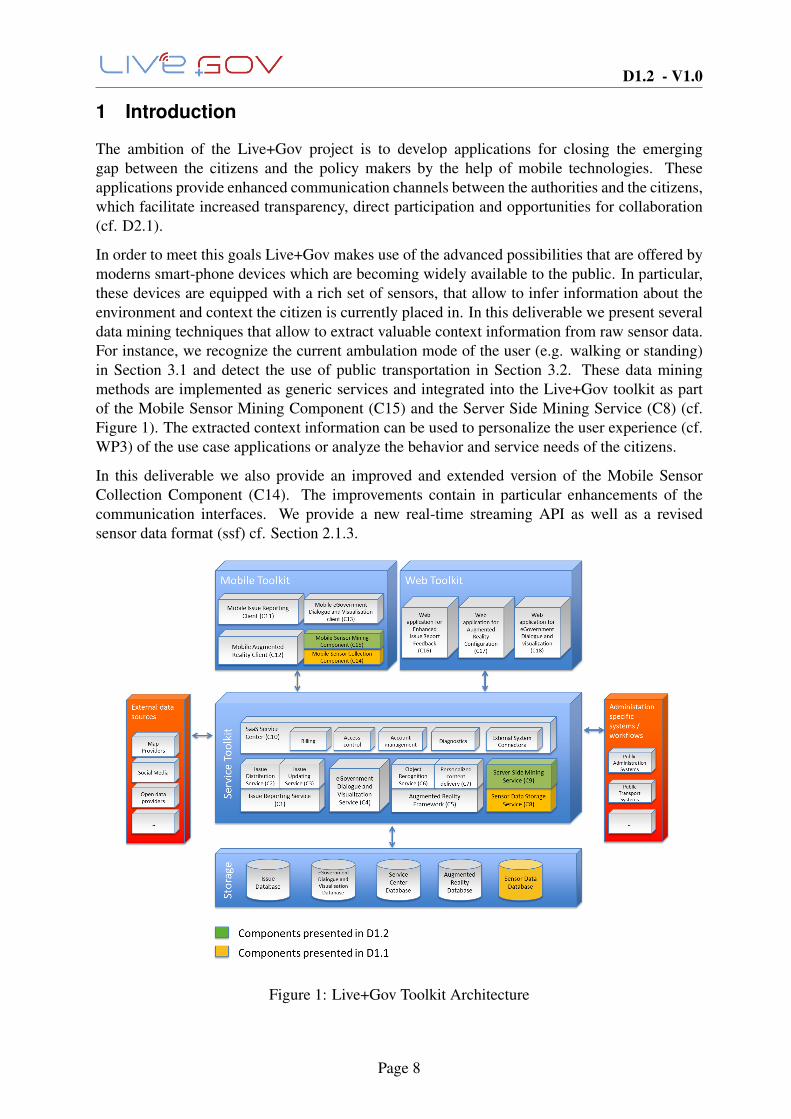
In order to meet this goals Live+Gov makes use of the advanced possibilities that are offered bymoderns smart-phone devices which are becoming widely available to the public. In particular,these devices are equipped with a rich set of sensors, that allow to infer information about theenvironment and context the citizen is currently placed in. In this deliverable we present severaldata mining techniques that allow to extract valuable context information from raw sensor data.For instance, we recognize the current ambulation mode of the user (e.g. walking or standing)in Section 3.1 and detect the use of public transportation in Section 3.2. These data miningmethods are implemented as generic services and integrated into the Live+Gov toolkit as partof the Mobile Sensor Mining Component (C15) and the Server Side Mining Service (C8) (cf.Figure 1). The extracted context information can be used to personalize the user experience (cf.WP3) of the use case applications or analyze the behavior and service needs of the citizens.
In this deliverable we also provide an improved and extended version of the Mobile SensorCollection Component (C14). The improvements contain in particular enhancements of thecommunication interfaces. We provide a new real-time streaming API as well as a revisedsensor data format (ssf) cf. Section 2.1.3.
Figure 1: Live+Gov Toolkit Architecture
Page 8

D1.2 - V1.0
2 Sensor Collection Service
2.1 Mobile Sensor Collector
In this chapter we present the a revised sensor collection component. It offers the followingimprovements over the last version presented in D1.1:
High performance recordings on Low-End devices During the field trial some low-enddevices showed difficulties to record the sensor samples with sufficient frequency. Westreamlined the architecture in order to reduce the overhead caused by the processing ofthe samples. For example, we traded the convenience of a SQL database in favor of theperformance benefits of a flat file solution.
Improved battery awareness Power consumption in the sensor collection process is largelydriven the GPS sensor. In May 2013 Google released a new location API, that takesadvantage of multiple location provider and reduces the power consumption significantly.The revised component makes use of this new API, and offers a fallback in case the serviceis not supported by the device.
Revised export format We have improved the data exchange formats used for publishingsamples to other components and storage on the central server. In Section 2.1.3 we specifythe ssf-Sensor Stream Format, which is inspired by the Common Log Format used bymany web servers. It allows easy human inspection and processing by standard (UNIX)tools like “grep” and “sed” while being reasonably memory efficient.
Streaming API The streaming API is a new communication channel between the mobile sensorcollector and the central server. It allows to transfer the incoming sensor data directly tothe server in real time.
Integration into Live+Gov Service Center The revised sensor collector and sensor storageservice is compatible with the Live+Gov service center. This feature allows central usermanagement as well as health monitoring and centralized log aggregation of the services.
Seamless Extendability The revised architecture can be easily extended by further streamprocessing components. This is realized by a dispatcher thread that distributes sensorsamples to registered components over a simple interface (again using ssf). Implementedextensions include the Human Activity Recognition component (c.f. section 3.1) and aGPS-sample publisher component that is used by the Service Line Detection service (cf.section 3.2).
2.1.1 Architecture Description
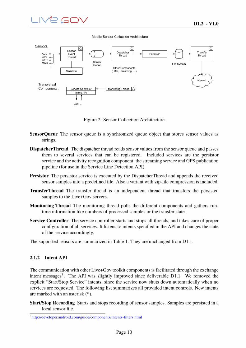
The new architecture is sketched in Figure 2. It allows asynchronous collection and processingof the collected sensor samples and can be easily extended by plugins which are executed by thedispatcher thread. It consists of the following individual components:
Sensor Event Thread The sensor event thread registers callback listeners for all configuredsensors. When sensor events occur, the received values are serialized in the ssf format (cf.2.1.3) and pushed onto the SensorQueue.
Page 9
D1.2 - V1.0
Figure 2: Sensor Collection Architecture
SensorQueue The sensor queue is a synchronized queue object that stores sensor values asstrings.
DispatcherThread The dispatcher thread reads sensor values from the sensor queue and passesthem to several services that can be registered. Included services are the persistorservice and the activity recognition component, the streaming service and GPS publicationpipeline (for use in the Service Line Detection API).
Persistor The persistor service is executed by the DispatcherThread and appends the receivedsensor samples into a predefined file. Also a variant with zip-file compression is included.
TransferThread The transfer thread is an independent thread that transfers the persistedsamples to the Live+Gov servers.
Monitoring Thread The monitoring thread polls the different components and gathers run-time information like numbers of processed samples or the transfer state.
Service Controller The service controller starts and stops all threads, and takes care of properconfiguration of all services. It listens to intents specified in the API and changes the stateof the service accordingly.
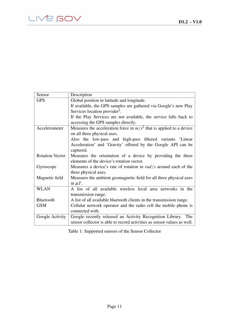
The supported sensors are summarized in Table 1. They are unchanged from D1.1.
2.1.2 Intent API
The communication with other Live+Gov toolkit components is facilitated through the exchangeintent messages3. The API was slightly improved since deliverable D1.1. We removed theexplicit “Start/Stop Service” intents, since the service now shuts down automatically when noservices are requested. The following list summarizes all provided intent controls. New intentsare marked with an asterisk (*).
Start/Stop Recording Starts and stops recording of sensor samples. Samples are persisted in alocal sensor file.
3http://developer.android.com/guide/components/intents-filters.html
Page 10
D1.2 - V1.0
Sensor DescriptionGPS Global position in latitude and longitude.
If available, the GPS samples are gathered via Google’s new PlayServices location provider2.If the Play Services are not available, the service falls back toaccessing the GPS samples directly.
Accelerometer Measures the acceleration force in m/s2 that is applied to a deviceon all three physical axes.Also the low-pass and high-pass filtered variants ’LinearAcceleration’ and ’Gravity’ offered by the Google API can becaptured.
Rotation Vector Measures the orientation of a device by providing the threeelements of the device’s rotation vector.
Gyroscope Measures a device’s rate of rotation in rad/s around each of thethree physical axes.
Magnetic field Measures the ambient geomagnetic field for all three physical axesin µT .
WLAN A list of all available wireless local area networks in thetransmission range.
Bluetooth A list of all available bluetooth clients in the transmission range.GSM Cellular network operator and the radio cell the mobile phone is
connected with.Google Activity Google recently released an Activity Recognition Library. The
sensor collector is able to record activities as sensor values as well.
Table 1: Supported sensors of the Sensor Collector
Page 11
D1.2 - V1.0
Delete Samples* Delete all stored samples on the device.
Send Annotation This intent allows users to annotate their recording by a string value that willbe recorded by a “tag-sensor”.
Enable/Disable Streaming* When enabled, all collected sensor samples are streamed over toa central server over the network. See section 2.1.4 for more details.
Transfer samples Controls the sample transfer state machine. When enabled and a networkconnection is available sensor samples are transferred in batches to the server backend.
Enable/Disable sample broadcast When enabled all recorded sensor samples are broadcastedin the form of intents into the system. This allows other components, e.g. featureextraction and context mining, to make use of the recorded sensor data.
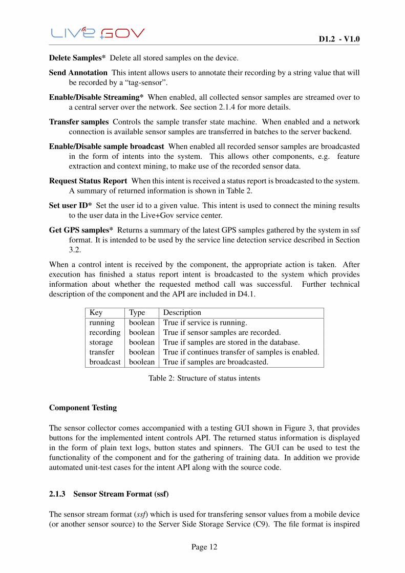
Request Status Report When this intent is received a status report is broadcasted to the system.A summary of returned information is shown in Table 2.
Set user ID* Set the user id to a given value. This intent is used to connect the mining resultsto the user data in the Live+Gov service center.
Get GPS samples* Returns a summary of the latest GPS samples gathered by the system in ssfformat. It is intended to be used by the service line detection service described in Section3.2.
When a control intent is received by the component, the appropriate action is taken. Afterexecution has finished a status report intent is broadcasted to the system which providesinformation about whether the requested method call was successful. Further technicaldescription of the component and the API are included in D4.1.
Key Type Descriptionrunning boolean True if service is running.recording boolean True if sensor samples are recorded.storage boolean True if samples are stored in the database.transfer boolean True if continues transfer of samples is enabled.broadcast boolean True if samples are broadcasted.
Table 2: Structure of status intents
Component Testing
The sensor collector comes accompanied with a testing GUI shown in Figure 3, that providesbuttons for the implemented intent controls API. The returned status information is displayedin the form of plain text logs, button states and spinners. The GUI can be used to test thefunctionality of the component and for the gathering of training data. In addition we provideautomated unit-test cases for the intent API along with the source code.
2.1.3 Sensor Stream Format (ssf)
The sensor stream format (ssf) which is used for transfering sensor values from a mobile device(or another sensor source) to the Server Side Storage Service (C9). The file format is inspired
Page 12

D1.2 - V1.0
Figure 3: Sensor collection testing GUI
by the Common Log Format used by many web servers. It replaces the XML-based formatused in D1.1. We view incoming sensor values as events and record them as a simple stream ofCSV-rows. Each sensor has an individual prefix but writes into the same file.
The key advantages of this format as opposed to the previously used XML format are:
• Human readability. The format is easy to understand by humans.
• Flexibility. Every line can be interpreted without the context of the file. Therefore ssf-filescan be arbitrarily sliced, concatenated and filtered using UNIX tools like grep, cat, sed,awk.
• Streaming support. Lines can be individually transferred over tcp sockets or messagingsystems. Allowing immediate inspection of the recorded samples on a remote system.
The rows of the ssf-format have the following structure in ABNF4:
SSF = SENSOR_PREFIX "," TIME_STAMP "," USER_ID "," SENSOR_VALUES
SENSOR_PRREFIX = "GPS" | "ACC" | "LAC" | "GRA" | "GYR" | "MAG" | \\"WIFI" | "BLT" | "GSM" | "ACT" | "ERR" | "TAG"
TIME_STAMP = *DIGITUSER_ID = *(ALPHA | DIGIT)SENSOR_VALUE = *VCHAR
4http://tools.ietf.org/html/rfc5234
Page 13
D1.2 - V1.0
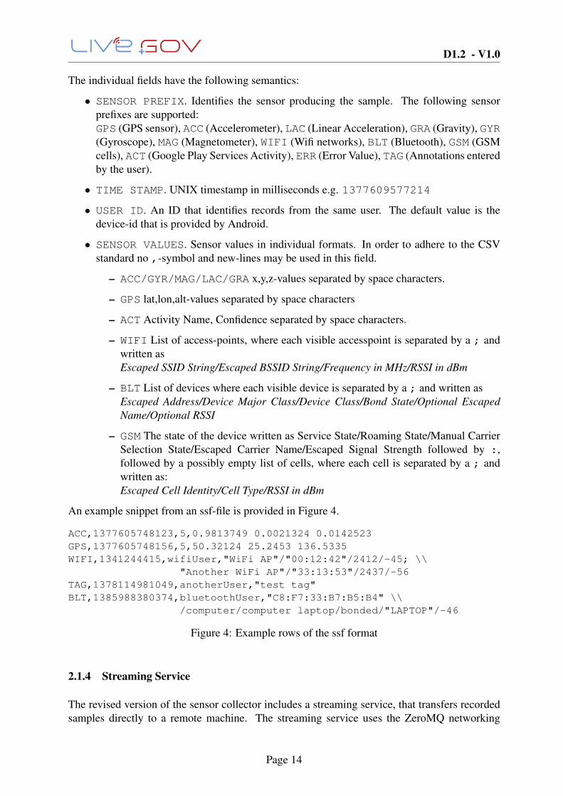
The individual fields have the following semantics:
• SENSOR PREFIX. Identifies the sensor producing the sample. The following sensorprefixes are supported:GPS (GPS sensor), ACC (Accelerometer), LAC (Linear Acceleration), GRA (Gravity), GYR(Gyroscope), MAG (Magnetometer), WIFI (Wifi networks), BLT (Bluetooth), GSM (GSMcells), ACT (Google Play Services Activity), ERR (Error Value), TAG (Annotations enteredby the user).
• TIME STAMP. UNIX timestamp in milliseconds e.g. 1377609577214
• USER ID. An ID that identifies records from the same user. The default value is thedevice-id that is provided by Android.
• SENSOR VALUES. Sensor values in individual formats. In order to adhere to the CSVstandard no ,-symbol and new-lines may be used in this field.
– ACC/GYR/MAG/LAC/GRA x,y,z-values separated by space characters.
– GPS lat,lon,alt-values separated by space characters
– ACT Activity Name, Confidence separated by space characters.
– WIFI List of access-points, where each visible accesspoint is separated by a ; andwritten asEscaped SSID String/Escaped BSSID String/Frequency in MHz/RSSI in dBm
– BLT List of devices where each visible device is separated by a ; and written asEscaped Address/Device Major Class/Device Class/Bond State/Optional EscapedName/Optional RSSI
– GSM The state of the device written as Service State/Roaming State/Manual CarrierSelection State/Escaped Carrier Name/Escaped Signal Strength followed by :,followed by a possibly empty list of cells, where each cell is separated by a ; andwritten as:Escaped Cell Identity/Cell Type/RSSI in dBm
An example snippet from an ssf-file is provided in Figure 4.
ACC,1377605748123,5,0.9813749 0.0021324 0.0142523GPS,1377605748156,5,50.32124 25.2453 136.5335WIFI,1341244415,wifiUser,"WiFi AP"/"00:12:42"/2412/-45; \\
"Another WiFi AP"/"33:13:53"/2437/-56TAG,1378114981049,anotherUser,"test tag"BLT,1385988380374,bluetoothUser,"C8:F7:33:B7:B5:B4" \\
/computer/computer laptop/bonded/"LAPTOP"/-46
Figure 4: Example rows of the ssf format
2.1.4 Streaming Service
The revised version of the sensor collector includes a streaming service, that transfers recordedsamples directly to a remote machine. The streaming service uses the ZeroMQ networking
Page 14
D1.2 - V1.0
Figure 5: Sensor Storage Architecture
library5 to transfer single ssf lines to the Live+Gov machine running a streaming server. Thestreaming server appends the received samples to a file (stream.ssf).
This simple service allows direct monitoring of the recorded samples, via simple UNIXcommand line tools.
tail -f stream.ssf prints the recoded samples to the console.grep <SENSOR PREFIX> filters out samples of a specific type.logtop shows the frequencies of the individual incoming sensor values.
2.2 Sensor Storage Service
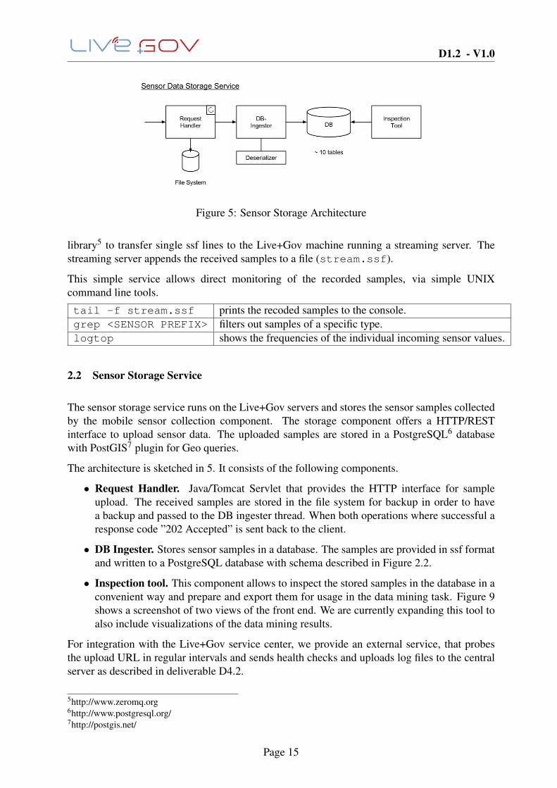
The sensor storage service runs on the Live+Gov servers and stores the sensor samples collectedby the mobile sensor collection component. The storage component offers a HTTP/RESTinterface to upload sensor data. The uploaded samples are stored in a PostgreSQL6 databasewith PostGIS7 plugin for Geo queries.
The architecture is sketched in 5. It consists of the following components.
• Request Handler. Java/Tomcat Servlet that provides the HTTP interface for sampleupload. The received samples are stored in the file system for backup in order to havea backup and passed to the DB ingester thread. When both operations where successful aresponse code ”202 Accepted” is sent back to the client.
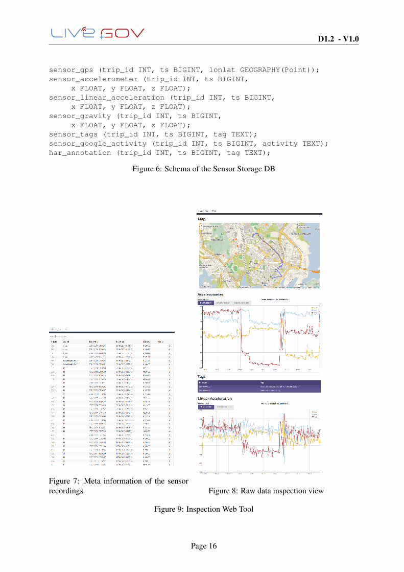
• DB Ingester. Stores sensor samples in a database. The samples are provided in ssf formatand written to a PostgreSQL database with schema described in Figure 2.2.
• Inspection tool. This component allows to inspect the stored samples in the database in aconvenient way and prepare and export them for usage in the data mining task. Figure 9shows a screenshot of two views of the front end. We are currently expanding this tool toalso include visualizations of the data mining results.
For integration with the Live+Gov service center, we provide an external service, that probesthe upload URL in regular intervals and sends health checks and uploads log files to the centralserver as described in deliverable D4.2.
5http://www.zeromq.org6http://www.postgresql.org/7http://postgis.net/
Page 15
D1.2 - V1.0
sensor_gps (trip_id INT, ts BIGINT, lonlat GEOGRAPHY(Point));sensor_accelerometer (trip_id INT, ts BIGINT,
x FLOAT, y FLOAT, z FLOAT);sensor_linear_acceleration (trip_id INT, ts BIGINT,
x FLOAT, y FLOAT, z FLOAT);sensor_gravity (trip_id INT, ts BIGINT,
x FLOAT, y FLOAT, z FLOAT);sensor_tags (trip_id INT, ts BIGINT, tag TEXT);sensor_google_activity (trip_id INT, ts BIGINT, activity TEXT);har_annotation (trip_id INT, ts BIGINT, tag TEXT);
Figure 6: Schema of the Sensor Storage DB
Figure 7: Meta information of the sensorrecordings Figure 8: Raw data inspection view
Figure 9: Inspection Web Tool
Page 16
D1.2 - V1.0
2.3 Cross-Platform Development
In order to reach as many citizens as possible with our efforts, it is important to have the mobilecomponents available on multiple platforms (e.g. Android, iOS). In deliverable D1.1 we haveevaluated different methods for mutiple platform sensor collection and reality mining. The basicthree possible pathways are (cf. D4.1):
1. Native development of all components for all platforms.
2. Web-based applications exploit HTML5 and advanced APIs offered by mobile browsersto provide services on the mobile phone.
3. Hybrid development uses native wrapper frameworks like PhoneGap8 or Titanium9 thatprovide access to native platform and hardware features.
The evaluation criteria included necessary sensor sampling frequencies, native communicationfacilities and support for background services. It was found, that the Titanium framework was isable to fulfill all three requirements. On the basis of this evaluation we proposed to implementthe mobile reality mining services using this framework.
In due course we have started to implement prototypes of sensor processing applications, suchas the TitaniumSensorCollector-package which is provided alongside with this deliverable. Itturned out, however, that it is not possible to collect sensor data while running in the backgroundwith Titanium. Our prior evaluation covered both requirements, but it was not tested if itwas cover both requirements at the same time. We were very surprised to learn that thoserequirements cannot be met in parallel.
For the practical use of the component, the support for sensor recordings in the backgroundis very important. Indeed, the classification of human activities is performed while the deviceis worn in a pocket, in which case the display is typically switched off and the application isrunning in the background.
As stated in D1.1, we propose independent native implementation as fallback solution in thiscase. Our initial development is focused on the Android platform. Using a conversion toolkit wehave been able to port some components (e.g. the sensor collector) to Blackberry. For supportof iOS further development is necessary.
It has to be noted, that independent native development is associated with high additional effort,as the development environments and APIs are very different from each other. It has to beassessed if the resources of the project shall be spent on this task, or rather in improving thequality of the existing Android implementations.
In the view of these difficulties we have taken steps to reduce the amount of computationperformed on the mobile device. In analogy to the image recognition task described in D3.1, itis possible to deploy parts of the logic on a central server. Currently our Service Line Detectioncomponent (c.f. section 3.2) is implemented in such a way, thereby paving the way for aniOS port of the Mobility Field Trial Application. A similar solution is planned for the HumanActivity Recognition Component described in section 3.1.
8http://phonegap.com/9http://www.appcelerator.com/
Page 17
D1.2 - V1.0
3 Reality Mining Methods
In this chapter we describe several reality mining methods that have been developed in theLive+Gov project.
The first three methods Human Activity Recognition (Section 3.1), Service Line Detection(Section 3.2) and Traffic Jam Detection (Section 3.3) are fully implemented and tested in fieldtrials. The work on Distributed Geo-Matching (Section 3.4) and Geographical Topic Analysis(Section 3.5) are of more scientific nature and have already lead to a publication [7].
3.1 Human Activity Recognition
In this section we describe the implementation of the human activity recognition (’HAR’)component on the mobile device. The algorithmic foundations of this data mining task have beendescribed in detail in deliverable D2.2 in section 3.2 “Mobile Sensing and activity recognition”.We include a brief summary here (3.1.1) for the sake of completeness. Subsection 3.1.2 containsthe descriptions of the implementation. In subsection 3.1.5 we evaluate our method on two datasets and compare it to the state of the art approaches.
3.1.1 HAR Method Summary
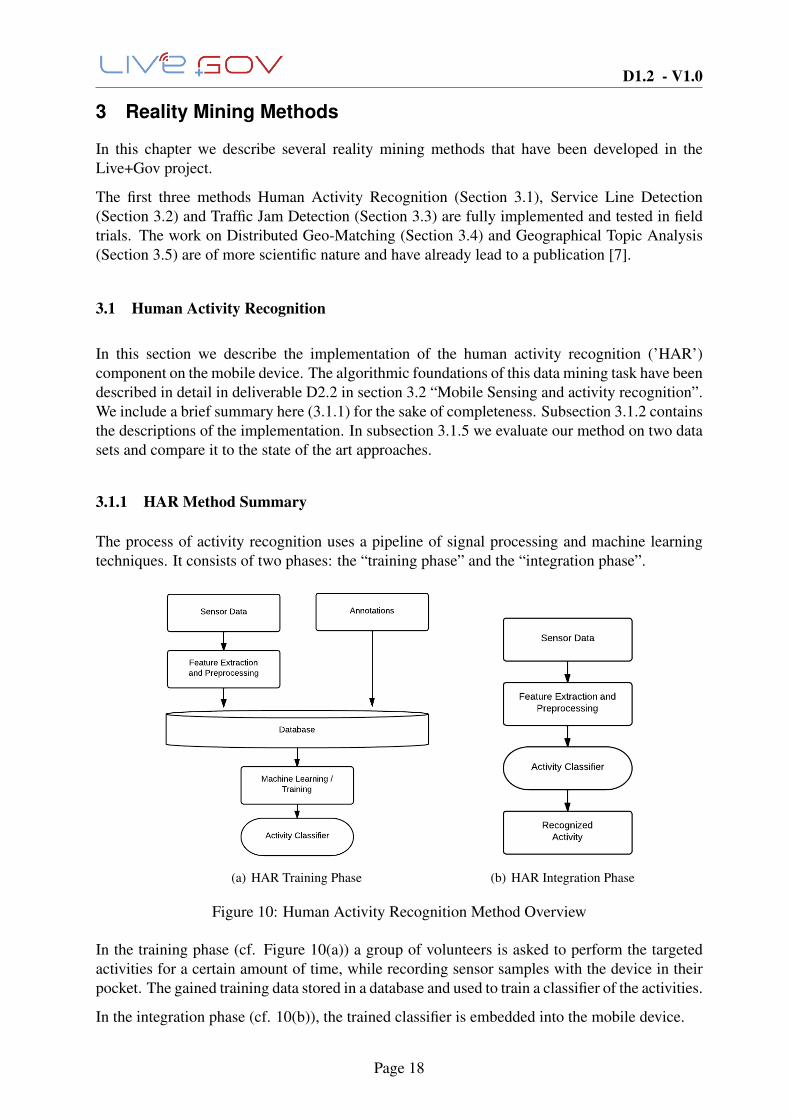
The process of activity recognition uses a pipeline of signal processing and machine learningtechniques. It consists of two phases: the “training phase” and the “integration phase”.
(a) HAR Training Phase (b) HAR Integration Phase
Figure 10: Human Activity Recognition Method Overview
In the training phase (cf. Figure 10(a)) a group of volunteers is asked to perform the targetedactivities for a certain amount of time, while recording sensor samples with the device in theirpocket. The gained training data stored in a database and used to train a classifier of the activities.
In the integration phase (cf. 10(b)), the trained classifier is embedded into the mobile device.
Page 18

D1.2 - V1.0
Both phases rely on the preprocessing steps of ”windowing” and “feature generation”. Thestream of incoming sensor data is divided into time windows of fixed size (typically 1-10 sec.)and for each window a set of features is computed. This features are filtering out relevantinformation from the raw signal. Typical features include mean values and standard deviationsas well as frequency domain features like Fourier modes.
Deliverable D2.2 contains detailed lists of all sensors and features and data mining methods thatare used in the literature as well as discussions of quality of the recognition results.
3.1.2 Component Description
The Human Activity Recognition Component implements the two phases described in Figure10. The training phase is executed offline on a server and uses the following processing pipeline(cf. Figure 11).
Figure 11: HAR Training Pipeline
1. Annotated Sensor Data. The training data is stored as ssf files in the file system. Theannotations are represented as folder structure. In this way it becomes very easy toadd new training data to the repository. Using the inspection web tool, one can selectappropriate time slices and export the corresponding samples as “.ssf” file. The exportedfile is then moved to the folder corresponding to the recorded activity.
2. Sample Producer. The sample producer service reads the sensor samples from the filesystem and pushes them onto a generic sample processing pipeline. The interface isdesigned a way that resembles the incoming data stream on the mobile device.
3. Window Producer. The window producer takes as constructor parameters a window-length and a delay. Incoming sensor samples are grouped in windows of the given lengthand passed further down as a single object.
4. Interpolation and Quality Check. The recorded sensor data can be subject soseveral irregularities, like frequency disparities or small outtakes. To ensure that thoseirregularities do not pollute the training data we perform quality checks on the individualwindows and interpolate the samples to a constant frequency of 50Hz.
5. Feature Calculation. The classification calculates different features extracted fromwindows of raw sampling data. A description of the used features is included in section3.1.3.
6. CSV-Persistor. The calculated feature vectors are stored on the file system as CSV file.
Page 19
D1.2 - V1.0
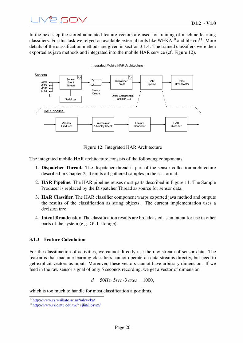
In the next step the stored annotated feature vectors are used for training of machine learningclassifiers. For this task we relyed on available external tools like WEKA10 and libsvm11. Moredetails of the classification methods are given in section 3.1.4. The trained classifiers were thenexported as java methods and integrated into the mobile HAR service (cf. Figure 12).
Figure 12: Integrated HAR Architecture
The integrated mobile HAR architecture consists of the following components.
1. Dispatcher Thread. The dispatcher thread is part of the sensor collection architecturedescribed in Chapter 2. It emits all gathered samples in the ssf format.
2. HAR Pipeline. The HAR pipeline reuses most parts described in Figure 11. The SampleProducer is replaced by the Dispatcher Thread as source for sensor data.
3. HAR Classifier. The HAR classifier component warps exported java method and outputsthe results of the classification as string objects. The current implementation uses adecision tree.
4. Intent Broadcaster. The classification results are broadcasted as an intent for use in otherparts of the system (e.g. GUI, storage).
3.1.3 Feature Calculation
For the classifiaction of activities, we cannot directly use the raw stream of sensor data. Thereason is that machine learning classifiers cannot operate on data streams directly, but need toget explicit vectors as input. Moreover, these vectors cannot have arbitrary dimension. If wefeed in the raw sensor signal of only 5 seconds recording, we get a vector of dimension
d = 50Hz ·5sec ·3 axes = 1000,
which is too much to handle for most classification algorithms.
10http://www.cs.waikato.ac.nz/ml/weka/11http://www.csie.ntu.edu.tw/∼cjlin/libsvm/
Page 20

D1.2 - V1.0
With the calculation of features, we try to reduce the dimensionality of the input signal, whilekeeping the essential information contained in the signal. We use two different methods forfeature calculation manual selection and an automated PCA based feature set.
Manually Selected Features
The following manual features have been selected:
Index Name Description0 id User ID of the recorded samples1 tag Name of the recoded activity2 xMean Mean values of the individual axes3 yMean4 zMean5 xVar Variance of the individual axes6 yVar7 zVar8 s2Mean Mean value of the length of the acceleration vector.9 s2Var Variance of the length of the acceleration vector
10 tilt Average tilting angle of the device towards the vertical axes.11 energy Total energy of the recording.12 kurtosis Kurtosis12 measure of ”peakedness” of the length of the acceleration
vector.13-24 S2Bins Histogram over the length of the acceleration vector.25-37 FFTBins Historgram over the absolute values of the Fourier Modes of the
length of the acceleration vector.
Our feature list has been guided by the literature (cf. D1.2, [9]). These consist of statisticalfeatures (mean and variance), that are computed for each of the three axes as well as for thelength of the acceleration vector s2 =
√x2 + y2 + z2. An explicit tilt-feature has been included
to allow better separation of the “sitting” and “standing” classes.
We also include frequency domain features. The “energy” feature measures the total spectraldensity13 of the signal. Furthermore a set of histogram features measures the energy of differentFourier modes of the signal. We have divided energy spectrum into 10 equally distributed bins,covering roughly 95% of the observed energy spectrum in the training data. Two more binsadded for outliers above and below the bin coverage.
PCA Based Features
There is a lot of freedom in the manual choice of feature vectors. Moreover, it is not clear thatthe heuristically selected features are able to separate the categories well. An automated wayof selecting features is provided by the Principal Component Analysis (PCA) method.14 Thismethod selects a number of linear features that maximize variance of the resulting data. We usea reduced vector size of 266 dimensions to keep 90% of the variance in our data set.
13http://en.wikipedia.org/wiki/Spectral density14http://en.wikipedia.org/wiki/Principal component analysis
Page 21
D1.2 - V1.0
3.1.4 Classifier Training
In this section we present more details about the employed machine learning methods for humanactivity recognition. Both methods rely on a training set of annotated feature vectors, and cannotbe used directly on the data-streams. As was explained in D2.1 the two presented methods arethe most popular approaches in the literature and have led to good classification accuracies inearlier work.
Decision Tree HAR classifier
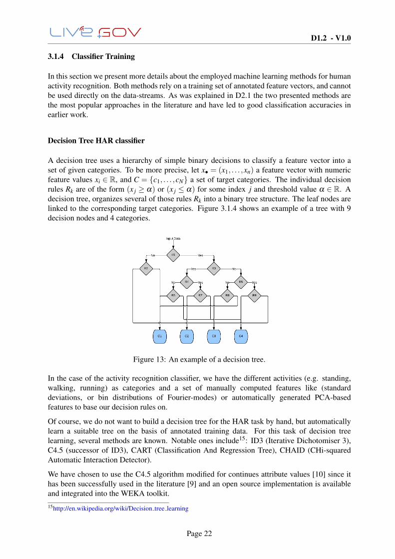
A decision tree uses a hierarchy of simple binary decisions to classify a feature vector into aset of given categories. To be more precise, let x• = (x1, . . . ,xn) a feature vector with numericfeature values xi ∈ R, and C = {c1, . . . ,cN} a set of target categories. The individual decisionrules Rk are of the form (x j ≥ α) or (x j ≤ α) for some index j and threshold value α ∈ R. Adecision tree, organizes several of those rules Rk into a binary tree structure. The leaf nodes arelinked to the corresponding target categories. Figure 3.1.4 shows an example of a tree with 9decision nodes and 4 categories.
Figure 13: An example of a decision tree.
In the case of the activity recognition classifier, we have the different activities (e.g. standing,walking, running) as categories and a set of manually computed features like (standarddeviations, or bin distributions of Fourier-modes) or automatically generated PCA-basedfeatures to base our decision rules on.
Of course, we do not want to build a decision tree for the HAR task by hand, but automaticallylearn a suitable tree on the basis of annotated training data. For this task of decision treelearning, several methods are known. Notable ones include15: ID3 (Iterative Dichotomiser 3),C4.5 (successor of ID3), CART (Classification And Regression Tree), CHAID (CHi-squaredAutomatic Interaction Detector).
We have chosen to use the C4.5 algorithm modified for continues attribute values [10] since ithas been successfully used in the literature [9] and an open source implementation is availableand integrated into the WEKA toolkit.
15http://en.wikipedia.org/wiki/Decision tree learning
Page 22

D1.2 - V1.0
The C4.5 algorithm uses the concept of information gain to build up a decision tree in a recursive,greedy fashion. For a set of annotated training vectors T = {(x•,c)|c∈C} a decision rule R splitsT into two subsets:
T = T+∪T−, T+ = {R(x•,c) = true}, T− = {R(x•,c) = false}
The information gain of this rule is defined as
IG(T,R) = H(T )− |T+||T |·H(T+)− |T
−||T |·H(T−),
where H(S) is the entropy of the collection S ⊂ T cf. [11]. The C4.5 algorithm finds thedecision rule with the largest information gain and uses this as the root for the decision tree. Itthen recurses into the subset T+ and T− and adds the generated nodes as childs to the root node.
The choice of the threshold values α for the decision rules is particularly crucial for the qualityof the trained decision tee. A possible improvement of the threshold selection algorithm can beobtained by pre-clustering of the attribute values before the training process cf. [8].
Figure 14 shows an example of a trained decision tree on manually generated features.J48 pruned tree------------------
Number of Leaves : 52
Size of the tree : 103
x18 <= 927| x24 <= 152| | x20 <= 211| | | x4 <= -2.936108| | | | x3 <= 1.132095| | | | | x18 <= 458| | | | | | x35 <= 2: WALKING (6.0/1.0)| | | | | | x35 > 2: CYCLING (2.0)| | | | | x18 > 458: SITTING (3.0)| | | | x3 > 1.132095: CYCLING (527.0)| | | x4 > -2.936108| | | | x4 <= 7.830095| | | | | x14 <= 13| | | | | | x18 <= 87| | | | | | | x2 <= 3.434441| | | | | | | | x3 <= -2.172633| | | | | | | | | x2 <= -3.51528: RUNNING (3.0/1.0)| | | | | | | | | x2 > -3.51528: WALKING (45.0/1.0)| | | | | | | | x3 > -2.172633: CYCLING (5.0/1.0)| | | | | | | x2 > 3.434441| | | | | | | | x19 <= 469: CYCLING (155.0)| | | | | | | | x19 > 469: WALKING (4.0/1.0)| | | | | | x18 > 87| | | | | | | x18 <= 415| | | | | | | | x15 <= 17| | | | | | | | | x34 <= 60| | | | | | | | | | x22 <= 138| | | | | | | | | | | x20 <= 98| | | | | | | | | | | | x21 <= 58: CYCLING (10.0)| | | | | | | | | | | | x21 > 58: WALKING (56.0)| | | | | | | | | | | x20 > 98| | | | | | | | | | | | x17 <= 108
// TRUNCATED
x18 > 927| x10 <= 0.58851: SITTING (1071.0)| x10 > 0.58851| | x3 <= -8.323328: WALKING (17.0)| | x3 > -8.323328: CYCLING (15.0/2.0)
Figure 14: Decision tree trained on manually computed features.
Support Vector Machine HAR Classifier
A popular algorithm to train a binary classification model for mapping features to activities is theSupport Vector Machines (SVMs). SVMs are known for their ability in smoothly generalizing
Page 23
D1.2 - V1.0
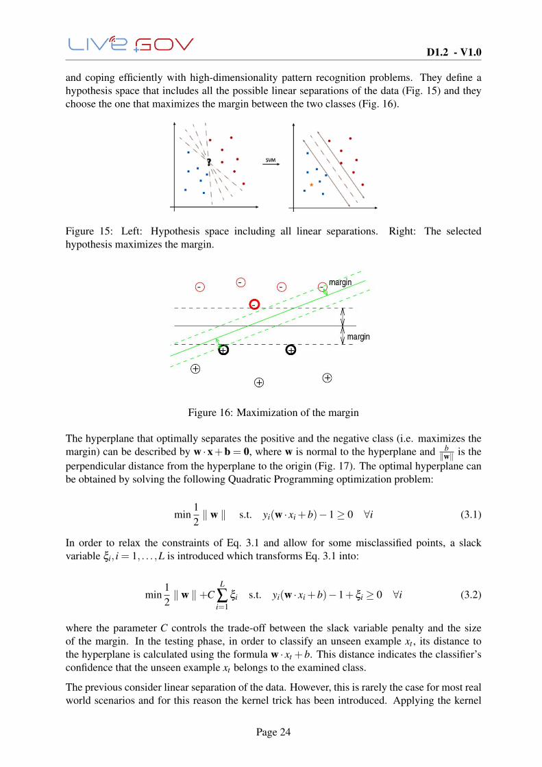
and coping efficiently with high-dimensionality pattern recognition problems. They define ahypothesis space that includes all the possible linear separations of the data (Fig. 15) and theychoose the one that maximizes the margin between the two classes (Fig. 16).
Figure 15: Left: Hypothesis space including all linear separations. Right: The selectedhypothesis maximizes the margin.
Figure 16: Maximization of the margin
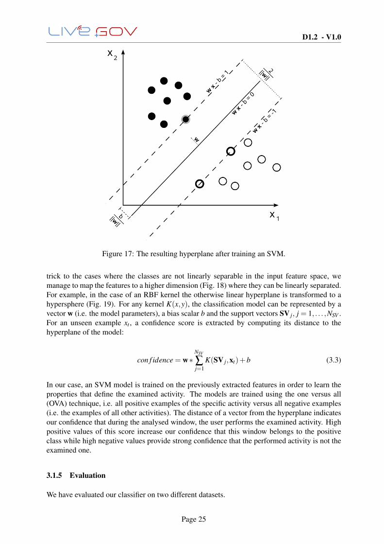
The hyperplane that optimally separates the positive and the negative class (i.e. maximizes themargin) can be described by w ·x+b = 0, where w is normal to the hyperplane and b
‖w‖ is theperpendicular distance from the hyperplane to the origin (Fig. 17). The optimal hyperplane canbe obtained by solving the following Quadratic Programming optimization problem:
min12‖ w ‖ s.t. yi(w · xi +b)−1≥ 0 ∀i (3.1)
In order to relax the constraints of Eq. 3.1 and allow for some misclassified points, a slackvariable ξi, i = 1, . . . ,L is introduced which transforms Eq. 3.1 into:
min12‖ w ‖+C
L
∑i=1
ξi s.t. yi(w · xi +b)−1+ξi ≥ 0 ∀i (3.2)
where the parameter C controls the trade-off between the slack variable penalty and the sizeof the margin. In the testing phase, in order to classify an unseen example xt , its distance tothe hyperplane is calculated using the formula w · xt +b. This distance indicates the classifier’sconfidence that the unseen example xt belongs to the examined class.
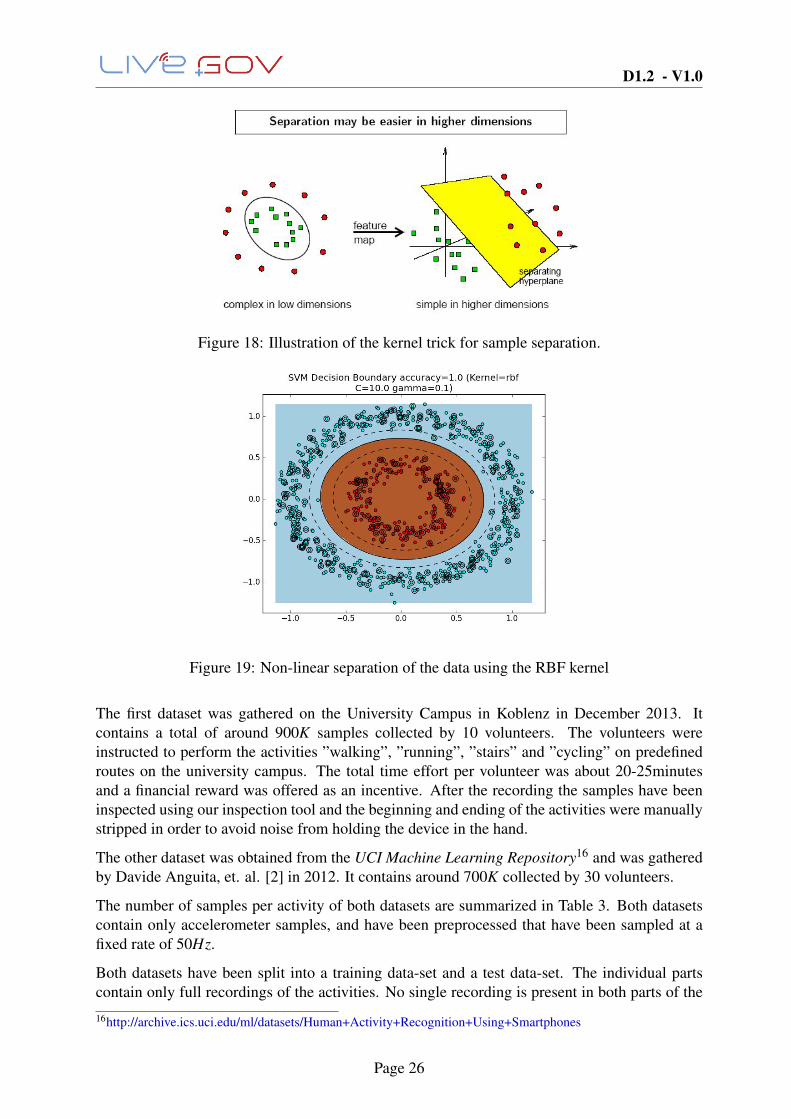
The previous consider linear separation of the data. However, this is rarely the case for most realworld scenarios and for this reason the kernel trick has been introduced. Applying the kernel
Page 24
D1.2 - V1.0
Figure 17: The resulting hyperplane after training an SVM.
trick to the cases where the classes are not linearly separable in the input feature space, wemanage to map the features to a higher dimension (Fig. 18) where they can be linearly separated.For example, in the case of an RBF kernel the otherwise linear hyperplane is transformed to ahypersphere (Fig. 19). For any kernel K(x,y), the classification model can be represented by avector w (i.e. the model parameters), a bias scalar b and the support vectors SV j, j = 1, . . . ,NSV .For an unseen example xt , a confidence score is extracted by computing its distance to thehyperplane of the model:
con f idence = w∗NSV
∑j=1
K(SV j,xt)+b (3.3)
In our case, an SVM model is trained on the previously extracted features in order to learn theproperties that define the examined activity. The models are trained using the one versus all(OVA) technique, i.e. all positive examples of the specific activity versus all negative examples(i.e. the examples of all other activities). The distance of a vector from the hyperplane indicatesour confidence that during the analysed window, the user performs the examined activity. Highpositive values of this score increase our confidence that this window belongs to the positiveclass while high negative values provide strong confidence that the performed activity is not theexamined one.
3.1.5 Evaluation
We have evaluated our classifier on two different datasets.
Page 25
D1.2 - V1.0
Figure 18: Illustration of the kernel trick for sample separation.
Figure 19: Non-linear separation of the data using the RBF kernel
The first dataset was gathered on the University Campus in Koblenz in December 2013. Itcontains a total of around 900K samples collected by 10 volunteers. The volunteers wereinstructed to perform the activities ”walking”, ”running”, ”stairs” and ”cycling” on predefinedroutes on the university campus. The total time effort per volunteer was about 20-25minutesand a financial reward was offered as an incentive. After the recording the samples have beeninspected using our inspection tool and the beginning and ending of the activities were manuallystripped in order to avoid noise from holding the device in the hand.
The other dataset was obtained from the UCI Machine Learning Repository16 and was gatheredby Davide Anguita, et. al. [2] in 2012. It contains around 700K collected by 30 volunteers.
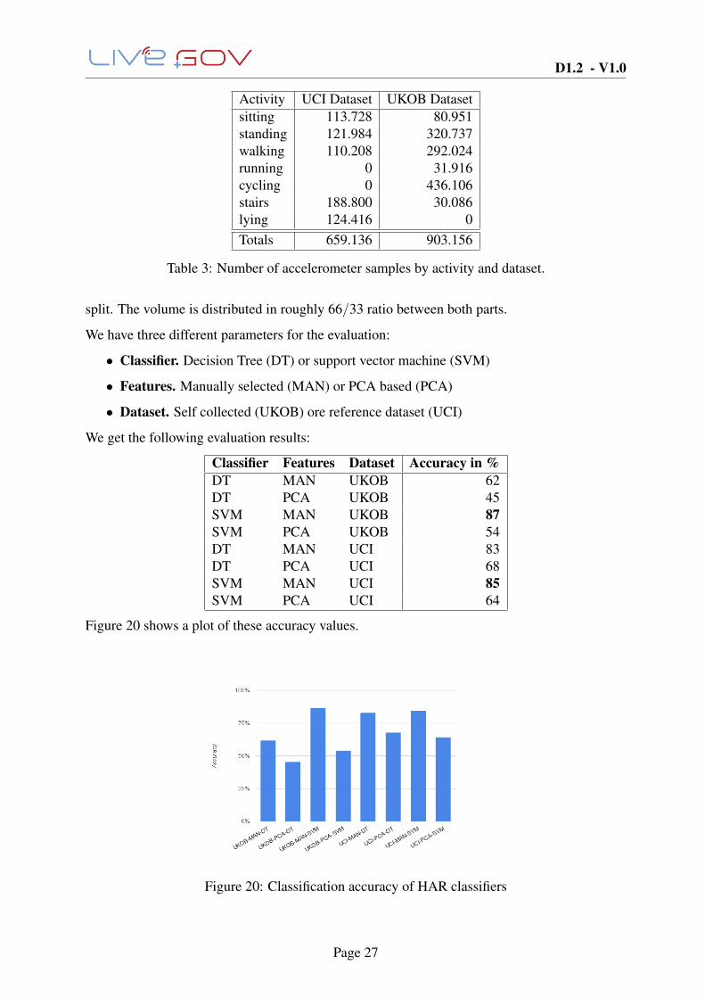
The number of samples per activity of both datasets are summarized in Table 3. Both datasetscontain only accelerometer samples, and have been preprocessed that have been sampled at afixed rate of 50Hz.
Both datasets have been split into a training data-set and a test data-set. The individual partscontain only full recordings of the activities. No single recording is present in both parts of the
16http://archive.ics.uci.edu/ml/datasets/Human+Activity+Recognition+Using+Smartphones
Page 26
D1.2 - V1.0
Activity UCI Dataset UKOB Datasetsitting 113.728 80.951standing 121.984 320.737walking 110.208 292.024running 0 31.916cycling 0 436.106stairs 188.800 30.086lying 124.416 0Totals 659.136 903.156
Table 3: Number of accelerometer samples by activity and dataset.
split. The volume is distributed in roughly 66/33 ratio between both parts.
We have three different parameters for the evaluation:
• Classifier. Decision Tree (DT) or support vector machine (SVM)
• Features. Manually selected (MAN) or PCA based (PCA)
• Dataset. Self collected (UKOB) ore reference dataset (UCI)
We get the following evaluation results:
Classifier Features Dataset Accuracy in %DT MAN UKOB 62DT PCA UKOB 45SVM MAN UKOB 87SVM PCA UKOB 54DT MAN UCI 83DT PCA UCI 68SVM MAN UCI 85SVM PCA UCI 64
Figure 20 shows a plot of these accuracy values.
Figure 20: Classification accuracy of HAR classifiers
Page 27
D1.2 - V1.0
These figures show, that we are still around 10% away from the state of the art classifier usedby [2] with 97% accuracy. There the authors use a multi-modal SVM on a similar list manuallyselected feature vectors and slightly parameters for window length and overlap. Our integratedapplication relies on a decision tree and manual features, which show significantly weakerperformance (64%) than state of the art in our experiments.
For both datasets the SVM trained on manual features performes best. Although there are severalparameters in the PCA feature extraction, that remain to be optimized, the evaluation resultssuggest that manually selected features yield better results. For the UCI dataset the decision treeis only slightly worse than the SVM based classifier whereas the UKob dataset shows a moresignificant drop of accuracy. This might be due to the fact that UKob dataset contains slightlydifferent activities than UCI, e.g. a large number samples is recorded for the cycling activity,which is not present at UCI, and conversely no samples for the lying task are present.
In conclusion, we have presented here a working HAR classification architecture, that has beenfully integrated into a mobile device and has been evaluated against state of the art classifiersfrom the literature on different datasets. Although the classification accuracies are still behindstate of the art, we are confident that we can improve our methods exploiting the built upinfrastructure.
Page 28
D1.2 - V1.0
3.2 Service Line Detection
One part of the user contextualization is the service line detection. The aim of this componentis to recognize if a citizen uses public transport within the HSL area in Helsinki. If sucha usage is detected, the right service line id with its direction and the further itinerary willbe determined. Based on this information it is possible to approach higher level problemslike network utilization analysis, personalized reports about traffic jams 3.3 and automatedconnecting train recommendations.
The service line detection is implemented as a server side component which provides a RESTAPI for answering user queries in real time. For long term evaluations all API calls are recordedand send to the Live+Gov Service Center on a daily bases. Due to the seamless integration intothe Live+Gov ecosystem, where each user gets an universal unique id, all received tracks arepersonalized and can be combined with additional information coming from other components.In a later analysis, the service line detection results can be augmented with the low level humanactivity recognition data of the same user to gain a better insight into the users behavior.
9:35
9:34
9:32
track coordinate with timestamp9:35
(a)
9:35 route A
9:35 route B
HSL realtime data9:35 route B
(b)
stop with time from time table
route path9:29
route A
route C
9:31
9:34
9:29
9:38
route B
9:44
9:42
(c)
12
3 4
5
678910 1
2
3
4
route A
route C
9:31
9:34
9:29
9:38
4
3
2
1
route B
9:44
9:42
stop with time from time table
interpolated coordinate1
29:29
(d)
12
3 4
5
678910 1
2
3
4
route A
route C
9:31
9:34
9:29
9:38
4
3
2
1
route B
9:44
9:42
stop with time from time table
interpolated coordinate1
29:29
9:33
9:32
9:30
9:319:32
9:33
9:34
9:35
9:36
9:37
9:43
9:43
interpolated coordinate with interpolated stop time
9:30
2
(e)
12
3 4
5
678910 1
2
3
4
route A
route C
9:31
9:34
9:29
9:38
4
3
2
1
route B
9:44
9:42
stop with time from time table
interpolated coordinate1
29:29
9:35
9:34
9:32
track coordinate with timestamp9:35
9:33
9:32
9:30
9:319:32
9:33
9:34
9:35
9:36
9:37
9:43
9:43
interpolated coordinate with interpolated timestamp
9:30
2
9:35 route A
9:35 route B
HSL realtime data9:35 route BCombined view of all data used for the HSL service line detection.
(f)
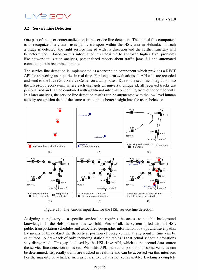
Figure 21: The various input data for the HSL service line detection.
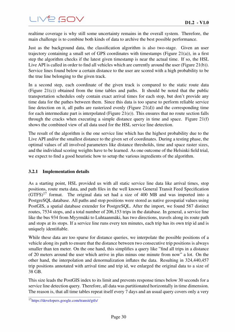
Assigning a trajectory to a specific service line requires the access to suitable backgroundknowledge. In the Helsinki case it is two fold: First of all, the system is fed with all HSLpublic transportation schedules and associated geographic information of stops and travel paths.By means of this dataset the theoretical position of every vehicle at any point in time can becalculated. A drawback of only including static time tables is that actual schedule deviationsstay disregarded. This gap is closed by the HSL Live API, which is the second data sourcethe service line detection relies on. With this API, the actual positions of some vehicles canbe determined. Especially trams are tracked in realtime and can be accessed via this interface.For the majority of vehicles, such as buses, live data is not yet available. Lacking a complete
Page 29
D1.2 - V1.0
realtime coverage is why still some uncertainty remains in the overall system. Therefore, themain challenge is to combine both kinds of data to archive the best possible performance.
Just as the background data, the classification algorithm is also two-stage. Given an usertrajectory containing a small set of GPS coordinates with timestamps (Figure 21(a)), in a firststep the algorithm checks if the latest given timestamp is near the actual time. If so, the HSLLive API is called in order to find all vehicles which are currently around the user (Figure 21(b)).Service lines found below a certain distance to the user are scored with a high probability to bethe true line belonging to the given track.
In a second step, each coordinate of the given track is compared to the static route data(Figure 21(c)) obtained from the time tables and paths. It should be noted that the publictransportation schedules only contain exact arrival times for each stop, but don’t provide anytime data for the pathes between them. Since this data is too sparse to perform reliable serviceline detection on it, all paths are rasterized evenly (Figure 21(d)) and the corresponding timefor each intermediate part is interpolated (Figure 21(e)). This ensures that no route section fallsthrough the cracks when executing a simple distance query in time and space. Figure 21(f)shows the combined view of all data used for the HSL service line detection.
The result of the algorithm is the one service line which has the highest probability due to theLive API and/or the smallest distance to the given set of coordinates. During a testing phase, theoptimal values of all involved parameters like distance thresholds, time and space raster sizes,and the individual scoring weights have to be learned. As one outcome of the Helsinki field trial,we expect to find a good heuristic how to setup the various ingredients of the algorithm.
3.2.1 Implementation details
As a starting point, HSL provided us with all static service line data like arrival times, stoppositions, route meta data, and path files in the well known General Transit Feed Specification(GTFS)17 format. The original data set had a size of 400 MB and was imported into aPostgreSQL database. All paths and stop positions were stored as native geospatial values usingPostGIS, a spatial database extender for PostgreSQL. After the import, we found 587 distinctroutes, 7534 stops, and a total number of 206,153 trips in the database. In general, a service linelike the bus 934 from Myyrmaki to Luhtaanmaki, has two directions, travels along its route pathand stops at its stops. If a service line runs every ten minutes, each trip has its own trip id and isuniquely identifiable.
While these data are too sparse for distance queries, we interpolate the possible positions of avehicle along its path to ensure that the distance between two consecutive trip positions is alwayssmaller than ten meter. On the one hand, this simplifies a query like ”find all trips in a distanceof 20 meters around the user which arrive in plus minus one minute from now” a lot. On theother hand, the interpolation and denormalization inflates the data. Resulting in 324,440,457trip positions annotated with arrival time and trip id, we enlarged the original data to a size of38 GB.
This size leads the PostGIS index to its limit and prevents response times below 30 seconds for aservice line detection query. Therefore, all data was partitionated horizontally in time dimension.The reason is, that all time tables repeat itself every 7 days and an usual query covers only a very
17https://developers.google.com/transit/gtfs/
Page 30

D1.2 - V1.0
small period of time at a specific weekday. Against this background, we divided the data into24 parts for every day, which results in 7 times 24 subtables in the database. Finally, this settingarchives average response times of less than one second for a whole service line detection query,containing of up to 200 single distance queries.
Page 31
D1.2 - V1.0
3.3 Traffic Jam Detection
In this section we are presenting a traffic jam detection module, that is able to detect irregularitiesin public transportation systems that provide real-time data about vehicles. It has been integratedinto the Live+Gov toolkit as part of the Server Side Mining Service (C9), and was successfullyused in the first Mobility Field Trial (cf. D5.1, D5.3) for the Helsinki metropolitan area.
3.3.1 Related work
Traffic fluency monitoring and jam detection is part of traffic control in all major cities and thereal time information about road network fluency is of interest to all network users and trafficrelated authorities. Over the last years, several different methods for detecting jams have beencreated. In many cities traffic is monitored via road side cameras detecting fluency in the mostimportant channels of the network and sends the image to authorities and web services. Anotherincreasingly popular method for detecting jams is by traffic message channels (TMC) that collectinformation about road network status from roadside sensors and vehicles and transmits theinformation via radio signals to the end user. TMC information is most commonly used innavigators, both on inbuilt vehicle navigating systems and separate navigator devices.18 Overthe past few years also different smartphone applications, such as Waze or Inrix have emergedon the market. In these applications information gathering is commonly done either with thevehicles connected to the system or by the users who report their journey conditions aroundthem. Different applications provide different type of information, usually including one orseveral of the following information types: jams, weather, road work and accidents. Whatis common to all known methods for detecting jams, no service is provided specifically to thepublic transport users as most services are targeted for private vehicle drivers and the authorities.Based on our surveys no service is being used specifically to public transport nor uses the delayinformation of public transport vehicles, which makes the traffic jam detection module an uniquetool.
3.3.2 Component Description
The jam detection module frequently polls vehicle location compared to the scheduled locationfrom the Helsinki public transport service. The module analyses the vehicle situation and detectswhere there are traffic jams in the certain transportation authoritys transportation area. Theinterface returns always the current jam situation, so client does not need to keep the jams inmemory.
The module detects the jams based the tram location, taking into notice the delay and how fastit increases. Also, the jam is only detected if there are several vehicles filling the same criteriawithin the same area.
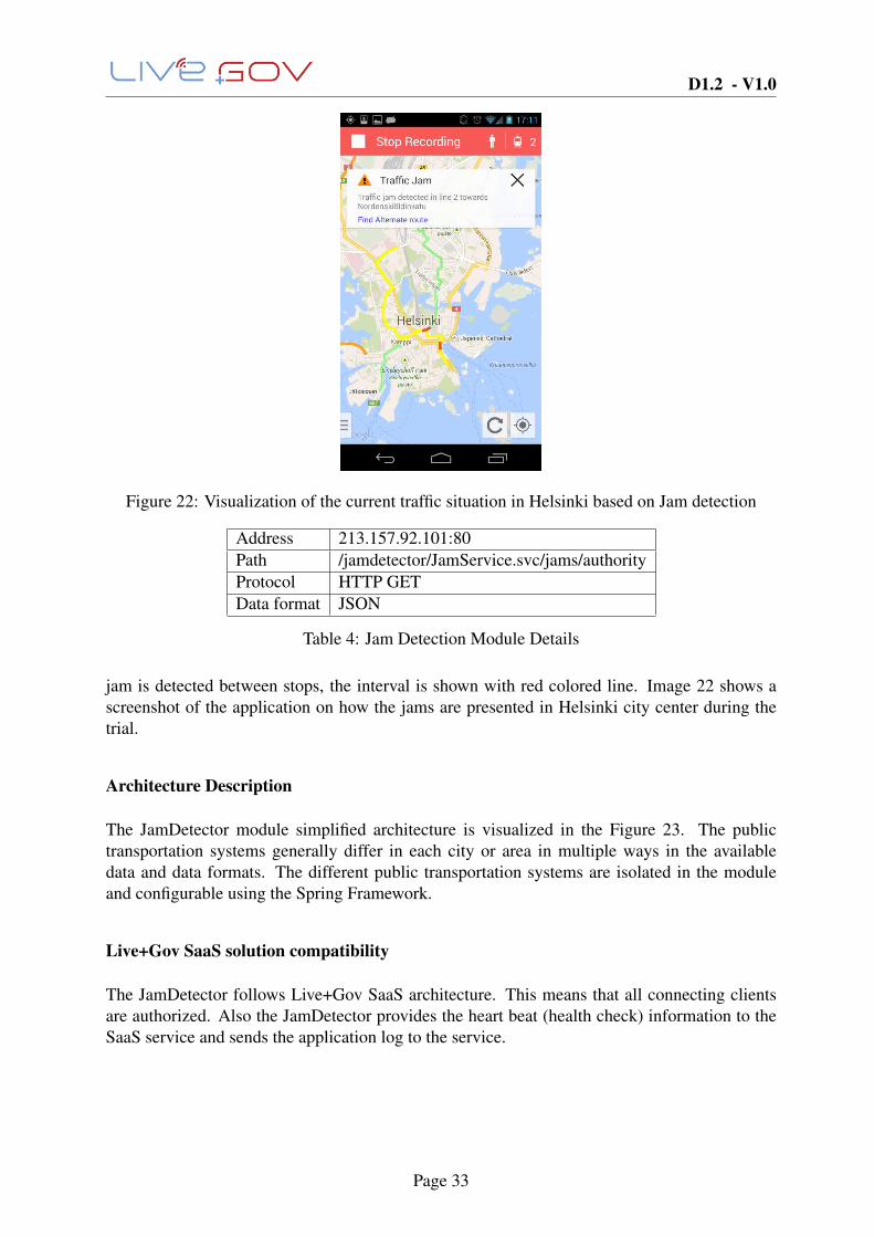
The module provides information about the nearest stop to the detected jam and also the previousstop from where the affected vehicles have come from. Based on this information current trafficsituation is visualized on the application. All of Helsinki city tram network can be drawn on themap, but only lines that are currently affected by trams are shown on the map at each time. Ifno jams are detected in between two stops, this interval is shown with green colored line. If a
18http://www.tisa.org/technologies/tmc/
Page 32
D1.2 - V1.0
Figure 22: Visualization of the current traffic situation in Helsinki based on Jam detection
Address 213.157.92.101:80Path /jamdetector/JamService.svc/jams/authorityProtocol HTTP GETData format JSON
Table 4: Jam Detection Module Details
jam is detected between stops, the interval is shown with red colored line. Image 22 shows ascreenshot of the application on how the jams are presented in Helsinki city center during thetrial.
Architecture Description
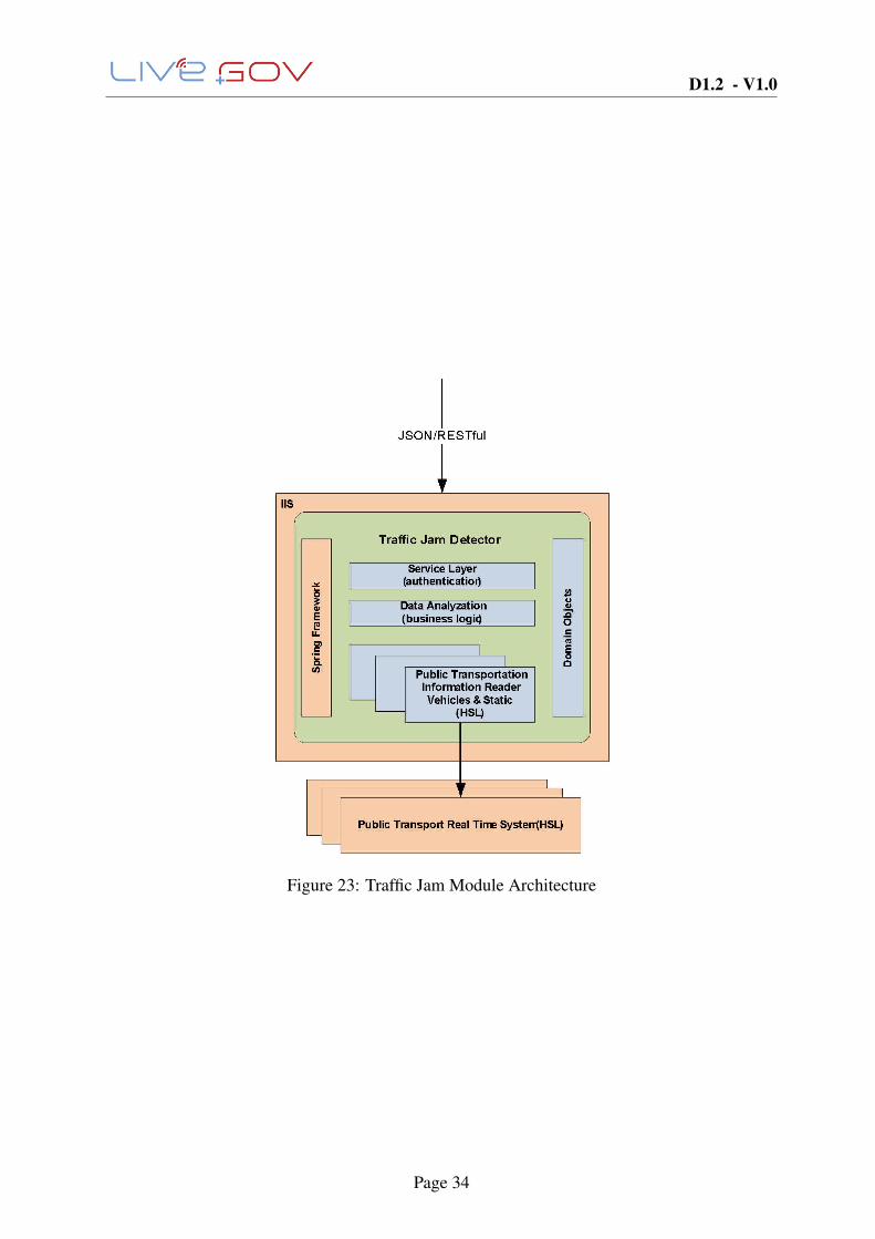
The JamDetector module simplified architecture is visualized in the Figure 23. The publictransportation systems generally differ in each city or area in multiple ways in the availabledata and data formats. The different public transportation systems are isolated in the moduleand configurable using the Spring Framework.
Live+Gov SaaS solution compatibility
The JamDetector follows Live+Gov SaaS architecture. This means that all connecting clientsare authorized. Also the JamDetector provides the heart beat (health check) information to theSaaS service and sends the application log to the service.
Page 33
D1.2 - V1.0
Figure 23: Traffic Jam Module Architecture
Page 34
D1.2 - V1.0
API description
The API lists the jams detected in the certain public transportation area in JSON format. Thejam object contains information about the vehicles participating the detected jam and vehiclesnearest stop/station. This information can be used to visualize the jam location for the users.
3.3.3 Evaluation
The module development begun with evaluating different methods for creating the detectionalgorithms and creating a way to detect jams reliably. The tram location data from Helsinkiprovides reliable information about the delay of a vehicle in real time and was considered themost efficient and reliable source of data for the jam detection.
A comprehensive and reliable detection algorithm was created through experimenting in theearly stages of the module development. The parameters to be used were searched the mostsuitable values through thorough consideration in order to generate reasonable and accuratealerts that would correspond with the logical situation in traffic and would fit in the definition ofa jam. After some weeks of monitoring the detections, the defined values were also re-evaluatedand re-defined before the first pilot based on the previous observations.
Based on the first trial results, the amount of detected jams is seen relatively high, on average 3jams were received on each time the API was called. This would indicate the parameters needingto be set tighter in the future if only greater jams are wanted to be detected. When evaluating theaccuracy it was quickly discovered that validating the detection is rather challenging when nothaving the possibility to verify the situation on site. User questionnaires showed that no userswere travelling in the areas where alerts were given at the time of the alert and therefore theycould not reliably state their opinion about the accuracy of alerts. Also, no known major jamstook place during the trial in the pilot area and therefore manual validation could not be doneduring the trial. Manual comparison to other known services providing jam alerts was done. Inall cases the detected jams were of a short duration, mainly less than a minute and thereforeno reliable statement about accuracy could be done at this stage. In the comparison we usedtwo popular services: Waze19, which is a mobile application providing traffic data in over 30countries and V-traffic20 , a national service in Finland for providing traffic data in major cities.Based on the comparison to other services the results seem promising as alerts were given in thesame areas at the same time, only with minor differences.
When comparing the module to existing services it is obvious that there are existing systems thatprovide information with more geographical coverage and collect the data from greater numberof sources. Thus, these services also provide more alerts as they also cover roads that are notincluded in the current module coverage, the Helsinki tram network. What needs to be addressedwhen comparing the module to existing services is that the other services do not focus on publictransport and using only these services would not help to meet the requirements of the mobilityuse case in full. However, the possibility to support the jam detection module with existingservices needs to be further studied.
We believe that when expanding the data to also cover other public transport vehicles, thecoverage in the module will increase and the quality and the usefulness of the module improves.
19http://www.inrixtraffic.com/20http://www.v-traffic.fi/
Page 35

D1.2 - V1.0
For example in the Helsinki region, all public transport busses, trams, trains and the ferry willbe covered in the new public transport information system to be implemented in 2016. Thenthe module will provide a much better service with greater geographical coverage and expandedfleet. Unfortunately at the time of development, location data is not yet available for othervehicles than trams but the possibility to include these vehicles in the jam detection has beentaken into notice from the start.
As no reliable evaluation is possible at this stage we will continue validating the module,analyzing the results and developing the algorithms. This process will continue until the finaltrial where improvements and reliable accuracy of the module are hoped to have been achieved.
Page 36
D1.2 - V1.0
3.4 Distributed Geo-Matching
Nowadays, the means of public transportation become equipped with physical sensors like GPSsensors or light barriers. Those sensors are used to keep track of the current vehicle position orto estimate the number of passengers. But those sensors do not detect, for instance, emergencies,accidents or the passengers’ opinions on bus lines. To overcome these limitations, another kindof sensors is required.
In the last decade, many social networks or micro-blogging services like TwitterTMarose. Theyare frequently used by humans to publish their opinions, observations, etc. which then canbe requested by a web API. Therefore, the users of those services can be seen as social sensors.The increasing number of mobile phones leads to a situation in which more and more passengersbecome social sensors by publishing statements about crowded buses or rioting passengers.
The evaluation of the social sensor data requires that the bus or train can be identified to whicha message is related. This task is simplified by the fact that most mobile phones have integratedGPS sensors. They measure the current geographical position, which is added to the publishedmessage together with a timestamp. This position information can be used to identify the nearesttrain or bus. A more detailed description of this matching problem will be given in the nextsection.
The amount of data produced by the different types of sensors can exceed the processingcapabilities of a single computer. Therefore, a distributed approach is required, which willbe explained in section 3.4.2.
3.4.1 Problem of Matching Physical and Social Sensor Data
In order to find the bus or train a message is related to, the data measured by the physical sensorshave to be processed first. In this context, the relevant data consists of the longitude and latitude(R×R) measured by the GPS sensors of the vehicles. Before transmitting these data, they haveto be extended by the unique id (Vid) of the current vehicle and a timestamp (T ) to keep track ofthe chronological order. The set of all possible position is defined as Pos in equation (3.4).
Pos := Vid×T ×R×R (3.4)
The relevant data of the social sensors are the messages published by the passengers. Eachmessage contains a timestamp, i.e., the publishing time and the GPS position of the mobilephone from which the message was sent. The set of all possible messages Mes is defined inequation (3.5) where C is the set of all possible message contents.
Mes := T ×R×R×C (3.5)
The data of the different sensors are transmitted as a not necessarily finite stream of data asdefined in the equations (3.6) and (3.7).
posStream : N→ Pos (3.6)mesStream : N→Mes (3.7)
The range of posStream, i.e., the set of vehicle positions received by the data stream posStreamare the trajectories of the different vehicles. A trajectory is defined in equation (3.8) as a discretefunction mapping some point in time to a geographical position.
tra j : T 7→ R×R (3.8)
Page 37
D1.2 - V1.0
But this definition is not adequate because the timestamps of messages may vary from thetimestamps contained in the position data of the vehicles. Therefore, a continuous trajectoryfunction tra j is required. This is reached by, for instance, a linear interpolation of tra j.
Equation (3.9) shows the function allTra j which maps the unique identifier of a vehicle on itscorresponding continuous trajectory.
allTra j : Vid 7→ (T 7→ R×R) (3.9)
In order to relate a message m to a bus or train, the vehicle must be determined which has thesmallest euclidean distance dist to the position of the sender at the point in time when m wassent. Furthermore, a vehicle has a maximum length maxDist and all vehicles with a greaterdistance from m can be ignored. Thus, each message can be seen as a range nearest-neighbourquery rnn as defined in equation (3.10).
rnn : Mes→ Pos∪{null} with (3.10)rnn((t, lonm, latm,cont)) := (vId, t, lonv, latv)
if allTra j(vId)(t) = (lonv, latv)∧dist((lonm, latm),(lonv, latv))≤ maxDist ∧6 ∃v′Id ∈Vid : dist((lonm, latm),allTra j(v′Id)(t))< dist((lonm, latm),allTra j(vId)(t))
rnn((t, lonm, latm,cont)) := null
otherwise
Putting it all together, the problem of finding the nearest vehicle for each message is defined asfollowed:
Problem Finding range nearest vehicle for each messageInput: posStream, mesStream, maxDistOutput: rnnStream : N→Mes×Pos• rnnStream(i) := (mesStream(i),rnn(mesStream(i)))
An implementation which solves this problem has to deal with the fact, that the data received bydifferent sensors are not equally delayed. For instance, the data measured from physical sensorsmay be faster transmitted then messages received from social networks.
Another difficulty is, that the amount of data received by the different input streams may exceedthe processing capabilities of a single computer. One solution for this problem would be todiscard incoming data if the load of the single machine would be to high. This could lead tothe loss of valuable data. In order to avoid this, a distributed approach is required which scaleshorizontally.
Some approaches like PLACE* [13] distribute the incoming data according to a static mappingof computers on geographical regions. The disadvantage of this static mapping can be seen, forinstance, if there exists a sport stadium in some region. If a sport event takes place, then there aremany vehicles and passengers producing a huge amount of data. Therefore, the correspondingcomputer can only deal with a relatively small region. But if no event takes place, this computerhas almost nothing to do. In order to improve this, the mapping has to be dynamic, i.e., adynamic load balancing is required.
3.4.2 Distributed Geo-Matching Approach
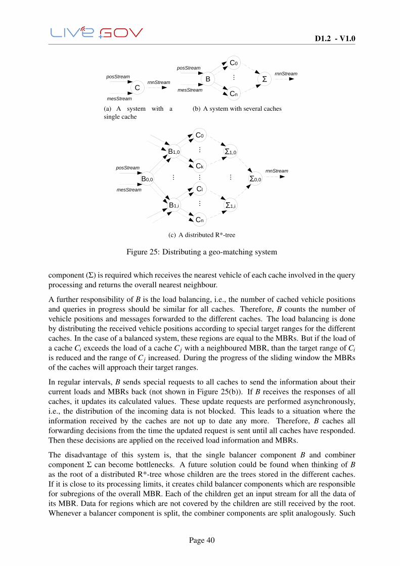
The schema of an intuitive stream-processing system which solves the problem described abovecan be seen in Figure 25(a). It consists of a single component (C) which receives the incoming
Page 38
D1.2 - V1.0
data streams of vehicle positions and messages. It caches the current positions and processes therange nearest-neighbour queries initiated by the received messages. The answers are transmittedvia the outgoing data stream rnnStream.
In order to answer range nearest-neighbour queries, C has to cache the current position of allvehicles. The problem of the delayed sensor data requires the caching of more vehicle positionsthan just the latest. Thus, a sliding window approach is implemented with a window sizeexceeding all regular delay times. This is realized by deleting all vehicle positions outside thewindow whenever a new position with a timestamp later then the timestamp of the latest cachedposition is received.
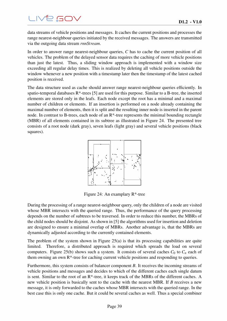
The data structure used as cache should answer range nearest-neighbour queries efficiently. Inspatio-temporal databases R*-trees [5] are used for this purpose. Similar to a B-tree, the insertedelements are stored only in the leafs. Each node except the root has a minimal and a maximalnumber of children or elements. If an insertion is performed on a node already containing themaximal number of elements, then it is split and the resulting inner node is inserted in the parentnode. In contrast to B-trees, each node of an R*-tree represents the minimal bounding rectangle(MBR) of all elements contained in its subtree as illustrated in Figure 24. The presented treeconsists of a root node (dark gray), seven leafs (light gray) and several vehicle positions (blacksquares).
Figure 24: An examplary R*-tree
During the processing of a range nearest-neighbour query, only the children of a node are visitedwhose MBR intersects with the queried range. Thus, the performance of the query processingdepends on the number of subtrees to be traversed. In order to reduce this number, the MBRs ofthe child nodes should be disjoint. As shown in [5] the algorithms used for insertion and deletionare designed to ensure a minimal overlap of MBRs. Another advantage is, that the MBRs aredynamically adjusted according to the currently contained elements.
The problem of the system shown in Figure 25(a) is that its processing capabilities are quitelimited. Therefore, a distributed approach is required which spreads the load on severalcomputers. Figure 25(b) shows such a system. It consists of several caches C0 to Cn each ofthem owning an own R*-tree for caching current vehicle positions and responding to queries.
Furthermore, this system consists of balancer component B. It receives the incoming streams ofvehicle positions and messages and decides to which of the different caches each single datumis sent. Similar to the root of an R*-tree, it keeps track of the MBRs of the different caches. Anew vehicle position is basically sent to the cache with the nearest MBR. If B receives a newmessage, it is only forwarded to the caches whose MBR intersects with the queried range. In thebest case this is only one cache. But it could be several caches as well. Thus a special combiner
Page 39
D1.2 - V1.0
C
posStream
mesStream
rnnStream
(a) A system with asingle cache
B
posStream
mesStream
ΣrnnStream
C0
Cn
...
(b) A system with several caches
B1,0 Σ1,0
C0
Ck
...B1,i Σ1,i
Cl
Cn
......
...B0,0
posStream
mesStream
Σ0,0
rnnStream...
(c) A distributed R*-tree
Figure 25: Distributing a geo-matching system
component (Σ) is required which receives the nearest vehicle of each cache involved in the queryprocessing and returns the overall nearest neighbour.
A further responsibility of B is the load balancing, i.e., the number of cached vehicle positionsand queries in progress should be similar for all caches. Therefore, B counts the number ofvehicle positions and messages forwarded to the different caches. The load balancing is doneby distributing the received vehicle positions according to special target ranges for the differentcaches. In the case of a balanced system, these regions are equal to the MBRs. But if the load ofa cache Ci exceeds the load of a cache C j with a neighboured MBR, than the target range of Ciis reduced and the range of C j increased. During the progress of the sliding window the MBRsof the caches will approach their target ranges.
In regular intervals, B sends special requests to all caches to send the information about theircurrent loads and MBRs back (not shown in Figure 25(b)). If B receives the responses of allcaches, it updates its calculated values. These update requests are performed asynchronously,i.e., the distribution of the incoming data is not blocked. This leads to a situation where theinformation received by the caches are not up to date any more. Therefore, B caches allforwarding decisions from the time the updated request is sent until all caches have responded.Then these decisions are applied on the received load information and MBRs.
The disadvantage of this system is, that the single balancer component B and combinercomponent Σ can become bottlenecks. A future solution could be found when thinking of Bas the root of a distributed R*-tree whose children are the trees stored in the different caches.If it is close to its processing limits, it creates child balancer components which are responsiblefor subregions of the overall MBR. Each of the children get an input stream for all the data ofits MBR. Data for regions which are not covered by the children are still received by the root.Whenever a balancer component is split, the combiner components are split analogously. Such
Page 40

D1.2 - V1.0
a system is illustrated in Figure 25(c).
Page 41
D1.2 - V1.0
3.5 Geographic Topic Analysis
The BuitenBeter dataset consists of 13,811 geo-tagged issues reported to the office of publicorder in the Netherlands between July and September 2012. Each issue is assigned to one of 16categories such as ”poor road conditions”, ”Dirt on the street” or ”Graffiti”.
Geographical co-occurrences of arbitrary categorical observations - such as public order issuesof the BuitenBeter dataset - can be used to discover latent underlying factors that explainobservations which co-occur more frequently than expected by chance. One method fordetecting these latent factors is probabilistic topic modelling, where grouped observations aremodelled as being sampled from mixtures of latent topics, which are probability distributionsover the set of distinct observations.
For the BuitenBeter dataset, we e.g. might expect that areas where graffities are reported willsee many reports of the category ”Dirt on the street” since both categories are related to urbanenvironments. We model those environments as hidden ”topics”.
Existing approaches for geographical topic modelling adopt topic models such as latent Dirichletallocation [6] and extend the models by assigning distributions over locations to topics, or byintroducing latent geographical regions. In models which extend topics for spatial distributions(such as two-dimensional normal distributions) [12], topics with a complex (i.e. non-Gaussian)spatial distribution cannot be detected. In models with latent, Gaussian distributed regions[14], documents within a complex shaped topic area do not influence the topic distribution ofdistant documents within the same area. Therefore, topics with a complex spatial distributionsuch as topics distributed along coastlines, rivers or country borders are harder to detect bysuch methods. More elaborate models introduce artificial assumptions about the structure ofgeographical distributions, e.g. by introducing hierarchical structures [1] in advance.
We introduce a novel geographical topic model which captures dependencies betweengeographical regions to support the detection of topics with complex, e.g. non-Gaussiandistributed spatial structures [7].
Our model differs from existing approaches in several aspects:
We model locations and words separately, as the separation of spatial clusters and documentsemantics allows us to define meaningful neighbour relations between spatially adjacent clusters.Our topic model takes a set of geographical clusters as input.
We also expect that geographical clusters adjacent in space exhibit similar topic distributions:Most geographical topics cannot be approximated by a simple spatial probability distributionsuch as a Gaussian distribution and for these complex topic areas, coherent sets of multiplespatial distributions are a reasonable approximation. Therefore we detect and smooth the topicdistribution of these adjacent regions to increase the probability of detecting coherent topic areas.
The detection of geographical clusters is straight-forward: We use a mixture of a fixed numberof Fisher distributions – distributions on a three dimensional unit sphere similar to isotropicGaussian distributions on a plane. The parameters are fit using the approximation given byBanerjee et al. [4] in an expectation-maximisation algorithm. In our model, each cluster isassociated with a distribution over the set of topics, sampled from a Dirichlet process (DP) witha common base measure which is itself drawn from a DP with Dirichlet distributed multinomialdistributions over the set of categories as base measure. For the smoothing of topic distributionsof adjacent clusters, we first define the adjacency relation using the Delaunay triangulation [3]
Page 42
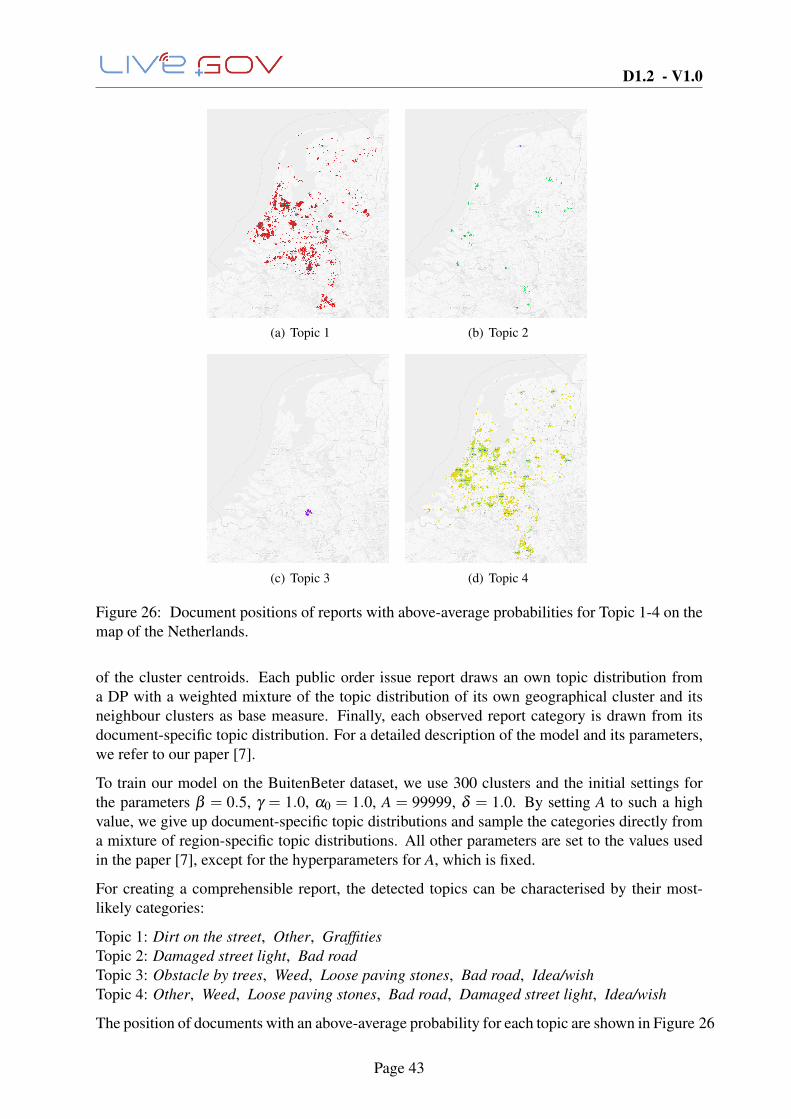
D1.2 - V1.0
(a) Topic 1 (b) Topic 2
(c) Topic 3 (d) Topic 4
Figure 26: Document positions of reports with above-average probabilities for Topic 1-4 on themap of the Netherlands.
of the cluster centroids. Each public order issue report draws an own topic distribution froma DP with a weighted mixture of the topic distribution of its own geographical cluster and itsneighbour clusters as base measure. Finally, each observed report category is drawn from itsdocument-specific topic distribution. For a detailed description of the model and its parameters,we refer to our paper [7].
To train our model on the BuitenBeter dataset, we use 300 clusters and the initial settings forthe parameters β = 0.5, γ = 1.0, α0 = 1.0, A = 99999, δ = 1.0. By setting A to such a highvalue, we give up document-specific topic distributions and sample the categories directly froma mixture of region-specific topic distributions. All other parameters are set to the values usedin the paper [7], except for the hyperparameters for A, which is fixed.
For creating a comprehensible report, the detected topics can be characterised by their most-likely categories:
Topic 1: Dirt on the street, Other, GraffitiesTopic 2: Damaged street light, Bad roadTopic 3: Obstacle by trees, Weed, Loose paving stones, Bad road, Idea/wishTopic 4: Other, Weed, Loose paving stones, Bad road, Damaged street light, Idea/wish
The position of documents with an above-average probability for each topic are shown in Figure 26 .
Page 43

D1.2 - V1.0
We see that, as expected, Topic 1 is only observed in the area of larger cities, whilst Topic 4 ispresent across the whole country. Topic 2 occurs mostly within city centres. Topic 3 is ob-served in the area of Eindhoven for which different categories were available in the BuitenBeterapplication.
Page 44

D1.2 - V1.0
4 Conclusion
In this deliverable we presented five different data mining methods for extracting contextinformation from the reality of citizens as well as an improved sensor collection architecture.
Three of these methods were integrated into the Live+Gov toolkit and tested in the field trial.Two methods are ongoing research projects, and have already led to a publication.
We have presented a Traffic Jam Detection component is able to detect irregularities in publictransportation systems, a Service Line Detection component that is capable of detecting theprecise service line used by a citizen, and a Human Activity Recognition component thatclassifies modes of human ambulation. These components have already shown acceptableperformance and will be improved further for the upcoming second field trials.
Page 45
D1.2 - V1.0
5 References
[1] Amr Ahmed, Liangjie Hong, and Alex Smola. Hierarchical geographical modeling of userlocations from social media posts. In WWW, 2013.
[2] Davide Anguita, Alessandro Ghio, Luca Oneto, Xavier Parra, and JorgeL. Reyes-Ortiz.Human activity recognition on smartphones using a multiclass hardware-friendly supportvector machine. In Jos Bravo, Ramn Hervs, and Marcela Rodrguez, editors, AmbientAssisted Living and Home Care, volume 7657 of Lecture Notes in Computer Science, pages216–223. Springer Berlin Heidelberg, 2012.
[3] Franz Aurenhammer. Voronoi diagrams – a survey of a fundamental geometric datastructure. ACM Comput. Surv., 23(3):345–405, 1991.
[4] Arindam Banerjee, Inderjit S. Dhillon, Joydeep Ghosh, and Suvrit Sra. Clustering on theunit hypersphere using von Mises–Fisher distributions. JMLR, 6:1345–1382, 2005.
[5] Norbert Beckmann, Hans-Peter Kriegel, Ralf Schneider, and Bernhard Seeger. The r*-tree:An efficient and robust access method for points and rectangles. In Proceedings of the 1990ACM SIGMOD International Conference on Management of Data, SIGMOD ’90, pages322–331, New York, NY, USA, 1990. ACM.
[6] David M. Blei, Andrew Y. Ng, and Michael I. Jordan. Latent Dirichlet allocation. JMLR,3:993–1022, March 2003.
[7] Christoph C. Kling, Jerome Kunegis, Sergej Sizov, and Steffen Staab. Detecting non-gaussian geographical topics in tagged photo collections. In WSDM, 2014.
[8] Sotiris Kotsiantis and Dimitris Kanellopoulos. Discretization techniques: A recent survey.GESTS International Transactions on Computer Science and Engineering, 32(1):47–58,2006.
[9] O. Lara and M. Labrador. A survey on human activity recognition using wearable sensors.Communications Surveys Tutorials, IEEE, PP(99):1–18, 2012.
[10] J. Ross Quinlan. Improved use of continuous attributes in c4. 5. Journal of ArtificialIntelligence Research, 1996.
[11] Claude E. Shannon. A mathematical theory of communication. 27(3):379–423, July 1948.
[12] Sergej Sizov. GeoFolk: latent spatial semantics in Web 2.0 social media. In WSDM, pages281–290, 2010.
[13] Xiaopeng Xiong, H.G. Elmongui, Xiaoyong Chai, and W.G. Aref. Place: A distributedspatio-temporal data stream management system for moving objects. In Mobile DataManagement, 2007 International Conference on, pages 44–51, 2007.
[14] Zhijun Yin, Liangliang Cao, Jiawei Han, Chengxiang Zhai, and Thomas S. Huang.Geographical topic discovery and comparison. In WWW, pages 247–256, 2011.
Page 46