DEMS: A Data Mining Based Technique to Handle Missing Data in Mobile Sensor Network Applications

Le Gruenwald Md. Shiblee Sadik Rahul Shukla Hanqing Yang

School of Computer ScienceUniversity of Oklahoma

Norman, Oklahoma, USAggruenwald@ou.edu

Outline

2

Research objective Current approaches The proposed approach: DEMS Performance Evaluation Conclusions and future work

Mobile Sensor Networks

3

A typical mobile sensor network: Sensor nodes are provided with motion capabilities Sensor nodes can relocate themselves Sensor nodes may move continuously/randomly Sensor nodes may move periodically to make up for

lost/missing sensors Sensor nodes send data to a base station.

Missing Sensor Data

4

Missing sensor data = sensor readings that fail to reach the base station or are corrupted when reaching the base station

Reasons for missing sensor data: Power shortage (sensor nodes are battery-powered) Mal-functioning of sensor nodes (hardware failure) Networking issues

Connection failures Data package collision

etc.

Research Objective

5

Goal: Develop an effective algorithm to estimate missing sensors’ readings in a mobile sensor network application.

Research Issues Issues common with static sensor networks:

Infiniteness, fast arrival rate, concept drifts

Additional issues: due to mobility of mobile sensors Spatial relations:

The spatial relation between two sensors’ readings is distorted by the mobility of mobile sensors

Temporal relations: The history data of a mobile sensor that are generated at different

locations may not necessarily possess the temporal relationships with the data in the current round of sensor readings

Frequent power failure Power outage is more common in mobile sensor network compared to

static sensor network because mobility requires excessive power.

6

Current Approaches

7

Ignore missing data

Ask the sensor again Add redundant sensors

Estimate missing data

Available approaches

Use average of other sensors

Use auto-regression model

Use some other statistics based model (e.g., Kalman filter)

Use data mining-based model

Fig 1. A taxonomy of techniques for handling missing data

Statistics based techniques

The Proposed Approach: DEMS

8

DEMS: Data Estimation for Mobile Sensors Based on two important concepts:

Virtual Static Sensor (VSS) A fictitious static sensor which mimics a real static sensor

helps reconstruct the spatial and temporal relations among the sensors’ readings

Association Rule Mining A popular method of discovering relationships among different items

helps explore the relationships among sensors’ readings.

DEMS Components DEMS has three major components:

Mapping Real Mobile Sensor (RMS) to Virtual Static Sensor (VSS) Divides the entire area of coverage into small hexagons A hexagon: the coverage area of a VSS with VSS being at the center of the

hexagon Converts RMS readings into VSS readings

Association rule mining Constructs a novel data structure called MASTER-tree to capture the association

rules among VSSs Updates MASTER-trees to capture the most recent association rules among

VSSs Data estimation

Uses the most recent association rules to estimate a missing VSS reading Uses the estimated value of the missing VSS reading as the value of the

missing RMS reading.

9

DEMS: Mapping RSS to VSS What is VSS?

A VSS is a fictitious static sensor A VSS reading is based on one or more RMSs’ readings A VSS has a unique identifier and has a unique area of

coverage Why do we need VSS?

Each VSS has a fixed location; hence the spatial relations among VSSs readings can be obtained

Each VSS reading is generated from a fixed location; hence history readings might have strong temporal relations with the current reading.

10

DEMS: Mapping RSS to VSS (Cont.)

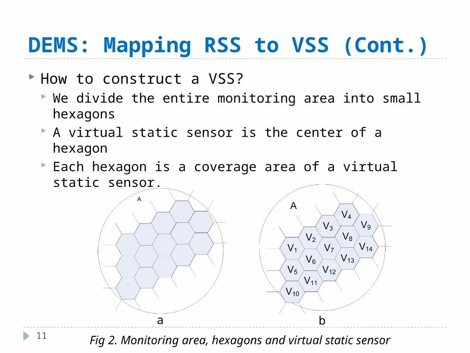
How to construct a VSS? We divide the entire monitoring area into small hexagons A virtual static sensor is the center of a hexagon Each hexagon is a coverage area of a virtual static sensor.

11 Fig 2. Monitoring area, hexagons and virtual static sensor

a b

DEMS: Mapping RMS to VSS

12

Goal: map RMSs’ readings to VSSs’ readings so that spatial and temporal relations among the sensor readings can be restored.

Two types of mapping: Mapping of a non-missing RMS to VSS Mapping of a missing RMS to VSS

Fig 3. RMSs and VSSs

DEMS: Mapping of a non-missing RMS to VSS If a VSS contains one RMS within its coverage area, the

RMS’s reading is used as the VSS reading If a VSS contains more than one RMSs, the average of the

RMSs’ readings is used as the VSS reading If a VSS contains no RMS, the VSS is called inactive.

13

DEMS: Mapping of a missing RMS to VSS Why mapping of a missing RMS is difficult?

RMS location is the key to RMS to VSS mapping If a RMS is missing, it is very likely that its data and location

would be missing together Hence mapping of a missing RMS to VSS requires intelligence

The solution A missing RMS is mapped to a VSS using a trajectory mining

approach for location prediction [Morzy, 2007].

14

DEMS: Mapping of a missing RMS to VSS (cont.) What is a trajectory?

A trajectory is the sequence of hexagons that a mobile sensor traverses

If a mobile sensor is not missing, it reports its location and the location is contained by one hexagon

Hence the sequence of hexagons is called a trajectory.

15 Fig 4. Trajectory of a RMS

(V14,V9,V11,V4,V3,V10) is the trajectory of M1

DEMS: Mapping of a missing RMS to VSS (cont.) Each RMS has a trajectory DEMS periodically stores the

trajectories (collected from all RMSs) into a frequency pattern tree

Frequency pattern tree It has a root labeled null Each node consists of an ID (hexagon ID)

and count (number of times it appears in the trajectories)

16

Example: 5 trajectories1. (V14, V9, V11, V4, V2, V8, V1)2. (V14, V9, V11, V4, V3, V10, V1)3. (V14, V9, V5, V4, V3, V10, V8)4. (V14, V9, V11, V4, V3, V10, V1, V8)5. (V2, V3, V6, V10, V8, V1) Fig 5. A frequency pattern tree

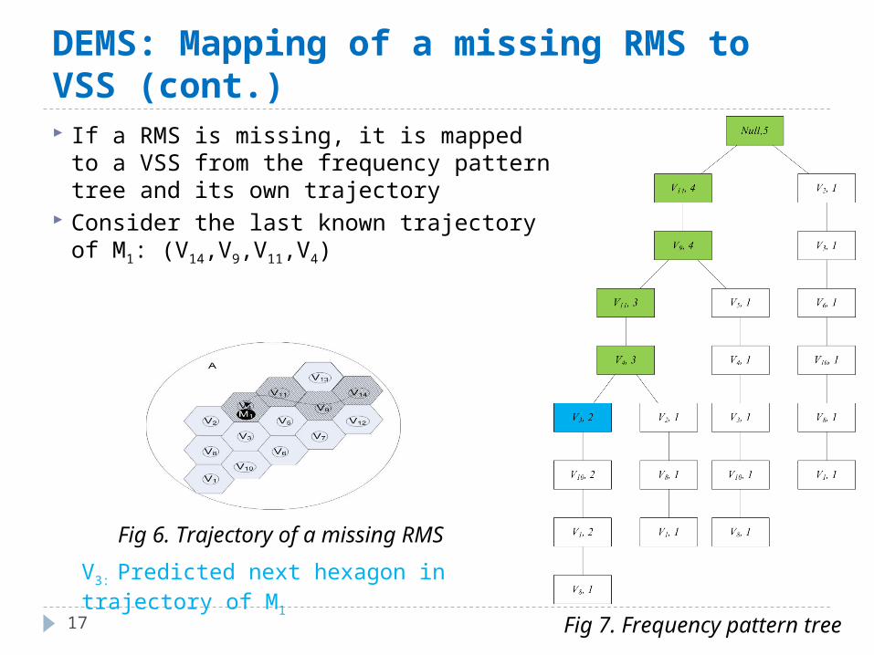
DEMS: Mapping of a missing RMS to VSS (cont.) If a RMS is missing, it is mapped to a VSS

from the frequency pattern tree and its own trajectory

Consider the last known trajectory of M1: (V14,V9,V11,V4)

17 Fig 7. Frequency pattern tree

Fig 6. Trajectory of a missing RMS

V3: Predicted next hexagon in trajectory of M1

DEMS: Mapping RMS to VSS (cont.)

18

Procedure mapReal2Virtual(RealSensorData listRSData, VirtualSensorData listVSData)

1 for each real sensor rs 2 if(rs is not missing)3 location ← listRSData(rs).Location4 vs ← findVirtualSensor(location)5 listVSData(vs).addReading(listRSData(rs).Reading)6 else7 location ← predictLocation(rs) 8 vs ← findVirtualSensor(location)9 listVSData(vs).status←missing

10 end loop11 for each virtual static sensor vs12 if(listVSData(vs) has data)13 listVSData(vs).status←active14 listVSData(vs).reading←average(listVSData(vs).Readings)15 else16 if(listVSData(vs).status is not missing)17 listVSData(vs).status ←inactive18 end loop

end procedure

Fig 8. Mapping algorithm

DEMS Components DEMS has three major components:

Real Mobile Sensor (RMS) to Virtual Static Sensor (VSS) Divides the entire area of coverage into small hexagons, Each hexagon is the coverage area of a virtual static sensor where the virtual

static sensor is assumed to be sitting in the middle of the hexagon, Converts RMS readings into VSS readings.

Association rule mining Constructs a novel data structure called MASTER-tree to capture the association

rules among VSSs Updates MASTER-trees to capture the most recent association rules among

VSSs. Data estimation

Uses the most recent association rules to estimate a missing VSS reading, Uses the missing VSS reading as missing RMS reading.

19

DEMS: Association Rule MiningGoal: mine and represent the potential

association rules among the VSS readings. We propose a novel data structure (called

MASTER-tree) to mine and represent the association rules among VSS readings

MASTER-tree basics: A MASTER-tree is capable of mining any kind

of association rules among any number of VSSs A MASTER-tree represents potential association

rules among the VSS readings A path in MASTER-tree represents a potential

association rule.

20

Fig 8. A MASTER-tree

DEMS: Association Rule Mining (cont.) The potential number of association rules among VSSs

grows exponentially with the number of VSSs To restrict the number of association rules, DEMS clusters

the VSSs into small groups and constructs one MASTER-tree for each group

DEMS uses Agglomerative clustering: Agglomerative clustering starts with every VSS as an

individual cluster At each step it merges two closest clusters based on their pair-

wise distances into one if the total number of VSSs in the new cluster does not exceed a user-defined maximum number of VSSs in one cluster.

21

DEMS: Association Rule Mining (cont.)

Fig 9. A MASTER-tree without the grid stricture

V2

Ø

V1 V3

V1 V3

V3 V1

V3 V2 V1 V2

V2

Details

DEMS: The MASTER-tree Projection Module (cont.)

23

Fig 10. MASTER-tree with grid structure

Ø

Summary StatsV2

Summary Stats

…Summary

StatsSummary

StatsV1

Summary Stats

…Summary

StatsSummary

StatsV3

Summary Stats

…Summary

Stats

Summary StatsV1

Summary Stats

…Summary

StatsSummary

StatsV3

Summary Stats

…Summary

Stats

Summary StatsV3

Summary Stats

…Summary

StatsSummary

StatsV1

Summary Stats

…Summary

Stats

Summary StatsV1

Summary Stats

…Summary

StatsSummary

StatsV3

Summary Stats

…Summary

Stats

Summary StatsV3

Summary Stats

…Summary

StatsSummary

StatsV1

Summary Stats

…Summary

Stats

V2[11, 20], V3[11, 20] → V1[1, 20]Support : 60%Confidence: 66%

DEMS: Association Rule Mining (cont.)

24

Fig 11. MASTER-tree with count

5

2V2 3 … 2V1 2 … 1 2V3 2 … 1

V1 2 … 1 V3 3 …

1V3 1 … 1V1 1 … 1

2V1… 2V3

…

V3 2 … 1V1 1 …

V2[1, 10], V1[1, 10] → V3[11, 20]Support : 40%Confidence: 100%

(2, 31, 485, 7657, 121937)

DEMS: Association Rule Mining (cont.)

25

Let The minimum support 50% The minimum confidence 50% A typical association rule becomes

V2[11, 20], V3[11, 20] → V1[1, 20]

The rule meaning: if the VSS reading of V2 is within 10 to 20 and the VSS reading for V3 is within 10 to 20, the VSS reading for V1 is most likely within 0 to 20.

There exists a path from the root node to V1[1, 20] via V2[11, 20] and V3[11, 20] in the Master-tree.

DEMS Components DEMS composed of three major components

Real Mobile Sensor (RMS) to Virtual Static Sensor (VSS) Divides the entire area of coverage into small hexagons, Each hexagon is the coverage area of a virtual static sensor where the virtual

static sensor is assumed to be sitting in the middle of the hexagon, Converts RMS readings into VSS readings.

Association rule mining Construct a novel data structure called MASTER-tree to capture the association

rules among VSSs, Update MASTER-trees to capture most recent association rules among VSSs.

Data estimation Uses the most recent association rules to estimate a missing VSS reading Uses the estimated value of the missing VSS reading as the estimated value of

the missing RMS reading.

26

DEMS: Data Estimation

Goal: estimate the missing VSS reading. The data estimation modules estimates the missing VSS The estimated reading for the missing VSS is used as the

estimated reading for the missing RMS.

27

DEMS: Data Estimation (cont.)

28

Fig 12. Flowchart of the data estimation module

(A step by step example)

Performance Evaluation

29

Simulation Model We simulate the missing data for our datasets A sensor is missing randomly (approximately 5-10%) for a consecutive

random number (10 - 20) of rounds Data and location both are missing for a missing sensor We use DEMS, TinyDB, SPIRIT and Average method to estimate

missing readings TinyDB

An average based technique which estimates the missing data by taking the average of the readings from other sensor readings in the current round.

SPIRIT An auto-regression based technique which estimates the missing data based on the

readings in the previous rounds Average

The average of other sensor readings is used as the estimated reading We compare the techniques based on mean absolute error (MAE)

MAE = Σ|estimation error|/number of estimations.

Performance Evaluation (cont.)

30

Datasets DAPPLE Project Dataset: A real life dataset

The carbon monoxide (CO) readings in the range [0, 6] were collected over a period of two weeks around Marylebone Road in London

The mobile sensors monitoring the atmospheric CO level are attached to PDAs which store these readings

We chose Thursday, 20th May 2004, when three sensors were simultaneously recording for about 32 minutes, resulting in 600 rounds (after disregarding the missing rounds) of CO readings

Factory Floor Temperature Dataset: A synthetic dataset A simulation of a mobile sensor network for monitoring factory floor temperatures Machines are placed on a floor Some machines are turned on for a number of rounds; the temperatures on these

machines reach a high constant temperature and heat disperse on the floor. 100 mobile sensors were roaming around in random directions to monitor the

factory floor and report the temperature readings in the range [0, 100C] from different locations.

The mobile sensor readings were sampled once per hour; the total rounds of readings are 5000 from 100 mobile sensors.

100 150 200 250 300 350 400 450 500 550 6000

0.2

0.4

0.6

0.8

1

1.2

1.4

1.6

1.8

2

Number of rounds

MA

E

Number o rounds vs. MAE

DEMS Average TinyDB SPIRIT

Performance Evaluation (cont.)

31

Fig 13. Impacts of number of rounds on MAE for DAPPLE project dataset

Approach Average MAE

DEMS 0

Average 1.2717

TinyDB 0.6331

SPIRIT 0.9437

Table 1. Average MAE for DAPPLE project dataset

500 1000 1500 2000 2500 3000 3500 4000 4500 50000

2

4

6

8

10

12

14

16

Number of rounds

MA

E

Number of rounds vs. MAE

DEMS Average TinyDB SPIRIT

Performance Evaluation (cont.)

32

Fig 14. Impacts of number of rounds on MAE for factory floor dataset

Approach Average MAE

DEMS 2.2538

Average 14.778

TinyDB 6.9621

SPIRIT 4.7472

Table 2. Average MAE for factory floor dataset

Conclusions and Future Work

33

We proposed DEMS: A novel data estimation technique for mobile sensor networks

based on data mining and virtual static sensor concepts Estimates missing sensor data with high accuracy

Future work: Extend DEMS to include Multiple base stations De-synchronized mobile sensor networks Cluster sensor networks.

Thanks

34

Questions?

MASTER-tree Construction

Ø

Fig . Merged tree for figure a and b

S2 S1 S3

S1 S3

S3

S3 S2 S1 S2

S2

Fig (a). A Pattern tree for S3

S2

Ø

S1 S3

S1 S3

S3

S3

Fig. (c) A Pattern tree for S1

S2

Ø

S3 S1

S3 S1

S1

S1

Fig (b). A Pattern tree for S1

S3

Ø

S1 S2

S1 S2

S2

S2

Ø

Fig . Merged tree for figure a, b and c

S2 S1 S3

S1 S3

S3 S1

S3 S2 S1 S2

S2

Back

MASTER-tree projection and data estimation:

An example

Simulation

Assume… Three Node (A, B, C) One dimension of Data (Temperature) Upper bound 30 lower bound 0, cell size = 10 dis(A,B) = 4, dis(A,C) = 3 and dis(B,C) = 5 MCSS = 10 minSup = 25% minConf = 75%

C

A B

Pattern trees

Ø

A B C

B C C

C

Ø

A C B

C B B

B

Ø

C B A

B A A

A

Ø

A B

B C

C B

A C

C

B A

AC

A BFinal MASTER tree without GS

Pattern tree for C Pattern tree for B Pattern tree for A

Data Sequence

A 4 14 11 18 6 8

B 8 18 15 22 10 12

C 7 17 14 21 9 ?

A B C

B C

A

A

A

BC

BC

Ø

A 4 14 11 18 6 8

B 8 18 15 22 10 12

C 7 17 14 21 9 ?

A B C

B C

A

A

A

BC

BC

Ø

A 4 14 11 18 6 8

B 8 18 15 22 10 12

C 7 17 14 21 9 ?

B C

C B

A C B

A

A

A B C

B C

A

A

A

BC

BC

Ø

A 4 14 11 18 6 8

B 8 18 15 22 10 12

C 7 17 14 21 9 ?

B C

C B

A C B

A

A

A B C

B C

A

A

A

BC

BC

Ø

A 4 14 11 18 6 8

B 8 18 15 22 10 12

C 7 17 14 21 9 ?

B C

C B

A C B

A

AC B

A C B

A

A

A B C

B C

A

A

A

BC

BC

Ø

A 4 14 11 18 6 8

B 8 18 15 22 10 12

C 7 17 14 21 9 ?

B C

C B

A C B

A

AC B

A C B

A

AC A

A B C

B C

A

A

A

BC

BC

Ø

A 4 14 11 18 6 8

B 8 18 15 22 10 12

C 7 17 14 21 9 ?

B C

C B

A C B

A

AC B

A C B

A

AC A

A B 2 2 1

B C

A

A

A

BC

BC

Ø

A 4 14 11 18 6 8

B 8 18 15 22 10 12

C 7 17 14 21 9 ?

B C

C B

A C B

A

AC B

A C B

A

AC A

MCSS = 10

Rule: Ø →C = [0, 29]Supp = 100%Conf = 100%

A B 2 2 1

B C

A

A

A

BC

BC

Ø

A 4 14 11 18 6 8

B 8 18 15 22 10 12

C 7 17 14 21 9 ?

B C

C B

A C B

A

AC B

A C B

A

AC A

MCSS = 10

Rule: Ø →C = [0, 19]Supp = 80%Conf = 80%

2 3 B 2 2 1

B 2

A

A

A

BC

BC

Ø

A 4 14 11 18 6 8

B 8 18 15 22 10 12

C 7 17 14 21 9 ?

B C

C B

A C B

A

AC B

A C B

A

AC A

MCSS = 10

Rule: Ø →C = [0, 29]Supp = 80%Conf = 80%

Rule: A →C = [0, 9]Supp = 40%Conf = 100%

Back to presentation