1

A Geometric Approach to Strapdown Magnetometer

Calibration in Sensor FrameJ.F. Vasconcelos, Member, IEEE, G. Elkaim, Member, IEEE, C. Silvestre Member, IEEE,

P. Oliveira Member, IEEE, and B. Cardeira Member, IEEE

Abstract

In this work a new algorithm is derived for the onboard calibration of three-axis strapdown magnetometers. The proposedcalibration method is written in the sensor frame, and compensates for the combined effect of all linear time-invariant distortions,namely soft iron, hard iron, sensor non-orthogonality, bias, among others. A Maximum Likelihood Estimator (MLE) is formulatedto iteratively find the optimal calibration parameters that best fit to the onboard sensor readings, without requiring external attitudereferences. It is shown that the proposed calibration technique is equivalent to the estimation of a rotation, scaling and translationtransformation, and that the sensor alignment matrix is given by the solution of the orthogonal Procrustes problem. Good initialconditions for the iterative algorithm are obtained by a suboptimal batch least squares computation. Simulation and experimentalresults with low-cost sensors data are presented and discussed, supporting the application of the algorithm to autonomous vehiclesand other robotic platforms.

Index Terms

Calibration; Magnetic fields; Maximum likelihood estimators; Least-squares algorithm.

I. INTRODUCTION

Magnetometers are a key aiding sensor for attitude estimation in low-cost, high performance navigation systems [1], [2], [3],

[4], with widespread application to autonomous air, ground and ocean vehicles. These inexpensive, low power sensors allow

for accurate attitude estimates by comparing the magnetic field vector observation in body frame coordinates with the vector

representation in Earth frame coordinates, available from geomagnetic charts and software [5]. In conjunction with vector

observations provided by other sensors such as star trackers or pendulums, the magnetometer triad yields complete 3-DOF

attitude estimation [3], [6].

The magnetic field reading distortions occur in the presence of ferromagnetic elements found in the vicinity of the sensor and

due to devices mounted in the vehicle’s structure. Other sources of disturbances are associated with technological limitations

in sensor manufacturing and installation. A comprehensive description of the magnetic compass theory can be found in [7].

Magnetometer calibration is an old problem in ship navigation and many calibration techniques have been presented in the

literature. The classic compass swinging calibration technique proposed in [8] is a heading calibration algorithm that computes

scalar parameters using a least squares algorithm. The major shortcoming of this approach is the necessity of an external

heading information [9], which is a strong requirement in many applications. A tutorial work using a similar but more sound

mathematical derivation is found in [7]. This book addresses the fundamentals of magnetic compass theory and presents a

methodology to calibrate the soft and hard iron parameters in heading and pitch, resorting only to the magnetic compass data.

However, the calibration algorithm is derived by means of successive approximations and is formulated in a deterministic

fashion that does not exploit the data of multiple compass readings.

In recent literature, advanced magnetometer calibration algorithms have been proposed to tackle distortions such as bias,

hard iron, soft iron and non-orthogonality directly in the sensor space, with no external attitude references and using optimality

criteria. The batch least squares calibration algorithm derived in [10], [9] accounts for non-orthogonality, scaling and bias errors.

A nonlinear, two-step estimator provides the initial conditions using a nonlinear change of variables to cast the calibration

in a pseudo-linear least squares form. The obtained estimate of the calibration parameters is then iteratively processed by a

linearized least squares batch algorithm.

The TWOSTEP batch method proposed in [11] is based on the observations of the differences between the actual and

the measured unit vector, denoted as scalar-checking. In the first step of the algorithm, the centering approximation derived

in [12] produces a good initial guess of the calibration parameters, by rewriting the calibration problem in a linear least

squares form. In a second step, a batch Gauss-Newton method is adopted to iteratively estimate the bias, scaling and non-

orthogonality parameters. In related work, [13] derives recursive algorithms for magnetometer calibration based on the centering

approximation and on nonlinear Kalman filtering techniques.

J.F. Vasconcelos, C. Silvestre, P. Oliveira and B.Cardeira are with the Institute for Systems and Robotics (ISR), Instituto Superior Tecnico, Lisbon, Portugal.E-mails: {jfvasconcelos, cjs, pjcro, bcardeira}@isr.ist.utl.pt Tel: (+351) 21-8418054, Fax: (+351) 21-8418291.G. Elkaim is with the Department of Computer Engineering, University of California Santa Cruz, 1156 High St., Santa Cruz, CA, 95064. E-mail:

elkaim@soe.ucsc.edu

2

Magnetic errors such as soft iron, hard iron, scaling, bias and non-orthogonality are modeled separately in [10]. Although

additional magnetic transformations can be modeled, it is known that some sensor errors are compensated by an equivalent

effect, e.g. the hard iron and sensor biases are grouped together in [9]. Therefore, the calibration procedure should address the

estimation of the joint effect of the sensor errors, as opposed to estimating each effect separately.

In this work, the magnetometer reading error model is discussed and cast in a error formulation which accounts for the

combined effect of all linear time-invariant magnetic transformations. A rigorous geometric formulation simplifies the problem

of compensating for the modeled and unmodeled magnetometer errors to that of the estimation of parameters lying on an

ellipsoid manifold. A complete methodology to calibrate the magnetometer is detailed, and a Maximum Likelihood Estimator

(MLE) allows for the formulation of the calibration problem as the optimization of the sensor readings likelihood.

The sensor calibration problem is naturally formulated in the sensor frame. The calibration parameters are estimated using

the magnetometer readings, and without resorting to external information or models about the magnetic field. In addition, a

closed form solution for the sensor alignment is also presented, based on the well known solution to the orthogonal Procrustes

problem [14].

The proposed calibration methodology is assessed both in simulation and using experimental data. Because the calibration

parameters are influenced by the magnetic characteristics of the payload, the geomagnetic profile of the terrain and diverse

vehicle operating conditions, the online calibration of the magnetometers is analyzed. The calibration parameters are estimated

for magnetometer data collected in ring shaped sets, corresponding to yaw and pitch maneuvers that are feasible for most land,

air and ocean vehicles. Simulation and experimental results show that the algorithm performs a computationally fast calibration

with accurate parameter estimation.

To the best of the authors’ knowledge, this work is an original rigorous derivation of a calibration algorithm using a

comprehensive model of the sensor readings in R3, that clarifies and exploits the geometric locus of the magnetometer readings,

given by an ellipsoid manifold. It is also shown that the calibration and alignment procedures are distinct.

This paper is organized as follows. In Section II, a unified magnetometer error parametrization is derived and formulated. It is

shown that the calibration parameters describe an ellipsoid surface and that the calibration and alignment problems are distinct.

A MLE formulation is proposed to calculate the optimal generic calibration parameters and an algorithm to provide good initial

conditions is presented. Also, a closed form solution for the magnetometer alignment problem is obtained. Simulation and

experimental results obtained with a low-cost magnetometer triad are presented and discussed in Section III. Finally, Section IV

draws concluding remarks and comments on future work.

II. MAGNETOMETER CALIBRATION AND ALIGNMENT

In this section, an equivalent parametrization of the magnetometer errors is derived. The main sources of magnetic distortion

and bias are characterized, to yield a comprehensive structured model of the magnetometer readings. Using this detailed

parametrization as a motivation, the magnetometer calibration problem is recast, without loss of generality, into a unified

transformation parametrized by a rotation R, a scaling S, and an offset b. Consequently, it is shown that for all linear

transformations of the magnetic field, such as soft and hard iron, non-orthogonality, scaling factor and sensor bias, the

magnetometer readings will always lie on an ellipsoid manifold.

A Maximum Likelihood Estimator formulation is proposed to find the optimal calibration parameters which maximize the

likelihood of the sensor readings. The proposed calibration algorithm is derived in the sensor frame and does not require any

specific information about the magnetic field’s magnitude and body frame coordinates. This fact allows for magnetometer

calibration without external aiding references. Also, a closed form optimal algorithm to align the magnetometer and body

coordinate frames is obtained from the solution to the orthogonal Procrustes problem.

A. Magnetometer Errors Characterization

The magnetometer readings are distorted by the presence of ferromagnetic elements in the vicinity of the sensor, the

interference between the magnetic field and the vehicle structure, local permanently magnetized materials, and by sensor

technological limitations.

Hard Iron / Soft Iron: The hard iron bias, denoted as bHI , is the combined result of the permanent magnets inherent to the

vehicle’s structure, as well as other elements installed in the vehicle, and it is constant in the vehicle’s coordinate frame.

Soft iron effects are generated by the interaction of an external magnetic field with the ferromagnetic materials in the vicinity

of the sensor. The resulting magnetic field depends on the magnitude and direction of the applied magnetic field with respect

to the soft iron material, producing

hSI = CSIBEREh (1)

where CSI ∈ M(3) is the soft iron transformation matrix, EBR is the rotation matrix from body to Earth coordinate frames,

BER := E

BR′, Eh is the Earth magnetic field,M(n,m) denotes the set of n×m matrices with real entries andM(n) := M(n, n).As described in [7, chapter XI], the combined hard and soft iron effects are given by hSI+HI = hSI +bHI . The linearization

of the ferromagnetic effects (1) yields the well known heading error δψ model [7], [9] adopted in compass swinging calibration,

3

which ignores the harmonics above 2ψ. The formulation (1), adopted in this paper, yields a rigorous approach to the simultaneousestimation of the hard and soft iron effects.

Non-orthogonality: The non-orthogonality of the sensors can be described as a transformation of vector space basis,

parametrized by [15]

CNO =

1 0 0sin(ψ) cos(ψ) 0− sin(θ) cos(θ) sin(φ) cos(θ) cos(φ)

(2)

where (ψ, θ, φ) are Yaw, Pitch and Roll Euler angles, respectively.Scaling and Bias: The null-shift or offset of the sensor readings is modeled as a constant vector bM ∈ R

3. The transduction

from the electrical output of the sensor to the measured quantity is formulated as a scaling matrix SM ∈ D+(3), where D(n)denotes the set of n× n diagonal matrices with real entries and D+(n) = {S ∈ D(n) : S > 0}.Wideband noise: The disturbing noise is assumed wideband compared with the bandwidth of the system, yielding uncorrelated

sensor sampled noise.

Alignment with the body frame: The formulation of the proposed algorithm in the sensor frame allows for sensor calibration

without determination of the alignment of the sensor with respect to a reference frame. An alignment procedure of the sensor

triad is proposed in this paper for the sake of completeness.

Other effects: Generic and more complex effects related to sensor-specific characteristics and to the magnetic distortion are

difficult to model accurately. The proposed calibration algorithm compensates for the combined influence of all linear time-

invariant transformations that distort the magnetic field, which are estimated in the form of an equivalent linear transformation.

B. Magnetometer Error Parametrization

In this section, an equivalent error model for the magnetometer readings is formulated. First, the estimation problem of

the non-ideal magnetic effects described in Section II-A is recast, without loss of generality, as the problem of estimating an

affine linear transformation. Second, it is shown that the linear transformation is equivalent to a single rotation, scaling and

translation transformation. In other words, to calibrate the magnetometer it is sufficient to estimate the center, orientation and

radii of the ellipsoid that best fit to the acquired data.

Define a sphere and an ellipsoid as [16]

S(n) = {x ∈ Rn+1 : ‖x‖2 = 1}, L(n) = {x ∈ R

n+1 : ‖SR′x‖2 = 1} (3)

where S ∈ D+(n+1) and R ∈ SO(n+1) describe the radii and orientation of the ellipsoid, respectively, and SO(n) = {R ∈O(n) : det(R) = 1}, O(n) = {U ∈ M(n) : UU′ = In×n}. The three-axis magnetometer reading is given by the Earth’smagnetic field Eh affected by the magnetic distortions and errors, yielding

hr i = SMCNO(CSIBERi

Eh + bHI) + bM + nm i (4)

where hr is the magnetometer reading in the (non-orthogonal) magnetometer coordinate frame, nm ∈ R3 is the Gaussian

wideband noise, SM , CNO, CSI , bHI and bM are the magnetic distortions described in Section II-A, and i = 1, . . . , ndenotes the index of the reading.

Without loss of generality, the magnetometer reading can be described by

hr i = CBhi + b + nm i (5)

whereC = SMCNOCSI , b = SMCNObHI+bM ,Bhi = B

ERiEh, Bhi ∈ S(2) is the magnetic field in body coordinate frame.

In particular, C ∈ M(3) and b ∈ R3 are unconstrained, so unmodeled linear time-invariant magnetic errors and distortions are

also taken into account.

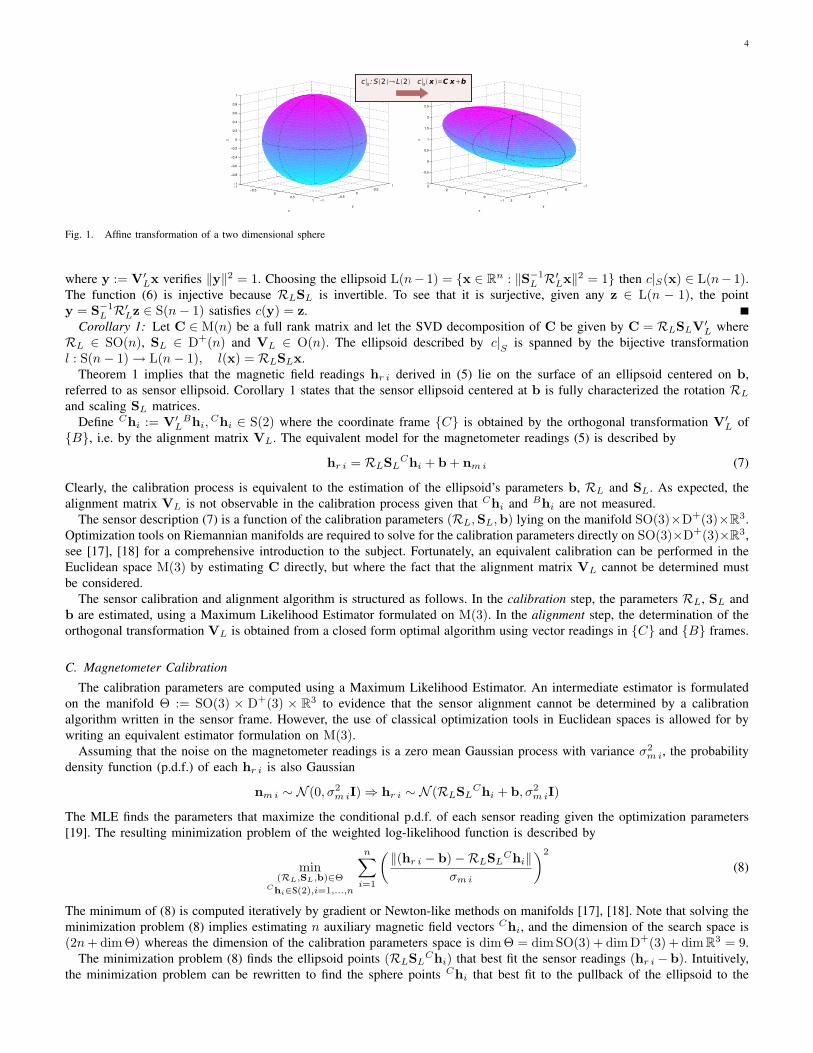
Given that the points Bhi are contained in the sphere, straightforward application of the Singular Value Decomposition

(SVD) [16] shows that the magnetometer readings hr i lie on an ellipsoid manifold, as illustrated in the example of Fig. 1 and

summarized in the following theorem. The proof is presented for the sake of clarity.

Theorem 1 ([16]): Let c : Rn → R

n, c(x) = Cx be a linear transformation where C ∈ M(n) is full rank. Then c(x) is abijective transformation between the sphere and an ellipsoid in R

n, i.e. there is an ellipsoid L(n−1) such that the transformationc|S : S(n− 1) → L(n− 1), c|S(x) = Cx is bijective.

Proof: Let the SVD decomposition C = UΣV′, where U,V ∈ O(n) and Σ ∈ D+(n). Define the matrices RL :=

UJ,SL := Σ,VL := VJ,J :=[

det(U) 0

0 In−1×n−1

]

, which describe a modified SVD decomposition with at least one special

orthogonal matrix C = RLSLV′L where RL ∈ SO(n), SL ∈ D+(n) and VL ∈ O(n). The transformation c(x) applied to the

sphere is given by

c|S(x) := RLSLy (6)

4

Fig. 1. Affine transformation of a two dimensional sphere

where y := V′Lx verifies ‖y‖2 = 1. Choosing the ellipsoid L(n− 1) = {x ∈ R

n : ‖S−1L R′

Lx‖2 = 1} then c|S(x) ∈ L(n− 1).The function (6) is injective because RLSL is invertible. To see that it is surjective, given any z ∈ L(n − 1), the pointy = S−1

L R′Lz ∈ S(n− 1) satisfies c(y) = z.

Corollary 1: Let C ∈ M(n) be a full rank matrix and let the SVD decomposition of C be given by C = RLSLV′L where

RL ∈ SO(n), SL ∈ D+(n) and VL ∈ O(n). The ellipsoid described by c|Sis spanned by the bijective transformation

l : S(n− 1) → L(n− 1), l(x) = RLSLx.

Theorem 1 implies that the magnetic field readings hr i derived in (5) lie on the surface of an ellipsoid centered on b,

referred to as sensor ellipsoid. Corollary 1 states that the sensor ellipsoid centered at b is fully characterized the rotation RL

and scaling SL matrices.

Define Chi := V′L

Bhi,Chi ∈ S(2) where the coordinate frame {C} is obtained by the orthogonal transformation V′

L of

{B}, i.e. by the alignment matrix VL. The equivalent model for the magnetometer readings (5) is described by

hr i = RLSLChi + b + nm i (7)

Clearly, the calibration process is equivalent to the estimation of the ellipsoid’s parameters b, RL and SL. As expected, the

alignment matrix VL is not observable in the calibration process given thatChi and

Bhi are not measured.

The sensor description (7) is a function of the calibration parameters (RL,SL,b) lying on the manifold SO(3)×D+(3)×R3.

Optimization tools on Riemannian manifolds are required to solve for the calibration parameters directly on SO(3)×D+(3)×R3,

see [17], [18] for a comprehensive introduction to the subject. Fortunately, an equivalent calibration can be performed in the

Euclidean space M(3) by estimating C directly, but where the fact that the alignment matrix VL cannot be determined must

be considered.

The sensor calibration and alignment algorithm is structured as follows. In the calibration step, the parameters RL, SL and

b are estimated, using a Maximum Likelihood Estimator formulated on M(3). In the alignment step, the determination of theorthogonal transformation VL is obtained from a closed form optimal algorithm using vector readings in {C} and {B} frames.

C. Magnetometer Calibration

The calibration parameters are computed using a Maximum Likelihood Estimator. An intermediate estimator is formulated

on the manifold Θ := SO(3) × D+(3) × R3 to evidence that the sensor alignment cannot be determined by a calibration

algorithm written in the sensor frame. However, the use of classical optimization tools in Euclidean spaces is allowed for by

writing an equivalent estimator formulation on M(3).Assuming that the noise on the magnetometer readings is a zero mean Gaussian process with variance σ2

m i, the probability

density function (p.d.f.) of each hr i is also Gaussian

nm i ∼ N (0, σ2m iI) ⇒ hr i ∼ N (RLSL

Chi + b, σ2m iI)

The MLE finds the parameters that maximize the conditional p.d.f. of each sensor reading given the optimization parameters

[19]. The resulting minimization problem of the weighted log-likelihood function is described by

min(RL,SL,b)∈Θ

Chi∈S(2),i=1,...,n

n∑

i=1

(

‖(hr i − b) −RLSLChi‖

σm i

)2

(8)

The minimum of (8) is computed iteratively by gradient or Newton-like methods on manifolds [17], [18]. Note that solving the

minimization problem (8) implies estimating n auxiliary magnetic field vectors Chi, and the dimension of the search space is

(2n+ dim Θ) whereas the dimension of the calibration parameters space is dim Θ = dim SO(3) + dim D+(3) + dim R3 = 9.

The minimization problem (8) finds the ellipsoid points (RLSLChi) that best fit the sensor readings (hr i −b). Intuitively,

the minimization problem can be rewritten to find the sphere points Chi that best fit to the pullback of the ellipsoid to the

5

sphere (S−1L R′

L(hr i − b)), yielding

min(RL,SL,b)∈Θ

Chi∈S(2),i=1,..,n

n∑

i=1

(

‖S−1L R′

L(hr i − b) − Chi‖

σm i

)2

(9)

The minimization problem (9) is suboptimal with respect to the unified error model (7), but can be rigorously derived using

a MLE formulation by assuming that the noise is external to the sensor, as detailed in the Appendix More important, the

log-likelihood function (9) can be optimized by searching only in the parameter space Θ.Proposition 1: The solution (R∗

L,S∗L,b

∗) of (9) also minimizes

min(RL,SL,b)∈Θ

n∑

i=1

(

‖S−1L R′

L(hr i − b)‖ − 1

σm i

)2

(10)

Proof: Given (R∗L,S

∗L,b

∗), the optimal Ch∗i satisfies

Ch∗i = argmin

Chi∈S(2)

‖v∗i − Chi‖

2 (11)

where v∗i := S∗−1

L R∗L′(hr i − b∗). The minimization problem (11) corresponds to the projection of v∗

i on the unit sphere,

which has the closed form solution Ch∗i =

v∗

i

‖v∗

i‖ . Therefore, the minimization problem (9) can be written as

min(RL,SL,b)∈Θ

n∑

i=1

(

‖S−1L RL

′(hr i − b) − vi

‖vi‖‖

σm i

)2

where vi := S−1L RL

′(hr i − b). Using simple algebraic manipulation produces the likelihood function (10).The minimization problem (10) can be formulated on the Euclidean space, which allows for the use of optimization tools

for unconstrained problems [20].

Proposition 2: Let (T∗,b∗T ) denote the solution of the unconstrained minimization problem

minT∈M(3)

n∑

i=1

(

‖T(hr i − bT )‖ − 1

σm i

)2

(12)

and take the SVD decomposition of T∗ = U∗T S∗

T V∗T′, UT ∈ O(3), ST ∈ D+(3), VT ∈ SO(3). The solution of (10) is given

by R∗L = V∗

T , S∗L = S∗

T−1, b∗ = b∗

T .

Proof: Using the equality ‖VLS−1L R′

L(hr i − b)‖ = ‖S−1L R′

L(hr i − b)‖ for any VL ∈ O(3), and the fact that, by theSVD decomposition, T := VLS−1

L R′L is a generic element of M(3), produces the desired results.

By Proposition 2, the calibration parameters of equation (7) are obtained by solving (12) and decomposing the resulting T∗.

Although (12) could be derived using (5), the intermediate derivations (9) and (10) where presented to show that (i) the sensor

readings lie on an ellipsoid manifold parametrized by RL, SL and b (ii) the alignment matrix, represented by VL (or U∗T )

cannot be determined in the calibration process, given that there are no body referenced measurements.

In this work, the minimization problem (12) is solved by using the gradient and Newton-descent method for Euclidean

spaces [20], and the Armijo rule for the step size determination. The gradient and Hessian of the log-likelihood function are

computed analytically and presented in the Appendix .

Given the calibration parameters (RL,SL,b), an unbiased and unit norm representation of the Earth magnetic field in thecalibration frame {C} is obtained by algebraic manipulation of (7), resulting in

Chi = S−1L R′

L(hr i − b). (13)

A good initial guess of the scaling and bias calibration parameters is produced by the two-step estimator proposed in [9].

The locus of measurements described by

‖Eh‖2 = ‖S−1(hr − b)‖2

is expanded and, by defining a nonlinear change of variables, it is rewritten as pseudo-linear least squares estimation problem

H(hr)f(b, s) = b(hr) (14)

where the matrix H(hr) ∈ M(n, 6) and the vector b(hr) ∈ Rn are nonlinear functions of the vector readings and the vector

of unknowns f(b, s) ∈ R6 is a nonlinear function of the calibration parameters. The closed form solution to the least squares

problem (14) is found to yield a good first guess of the calibration parameters [15].

In alternative, the algorithm proposed in [21] can produce an initial ellipsoid guess based on the difference-of-squares error

criterion using a semidefinite programming (SDP) formulation. However, the SDP algorithm is computationally feasible only for

no more than a few hundred samples, whereas the pseudo-linear least squares formulation (14) allows for efficient processing

of the several thousands of points contained in the calibration data, which are required in practice.

6

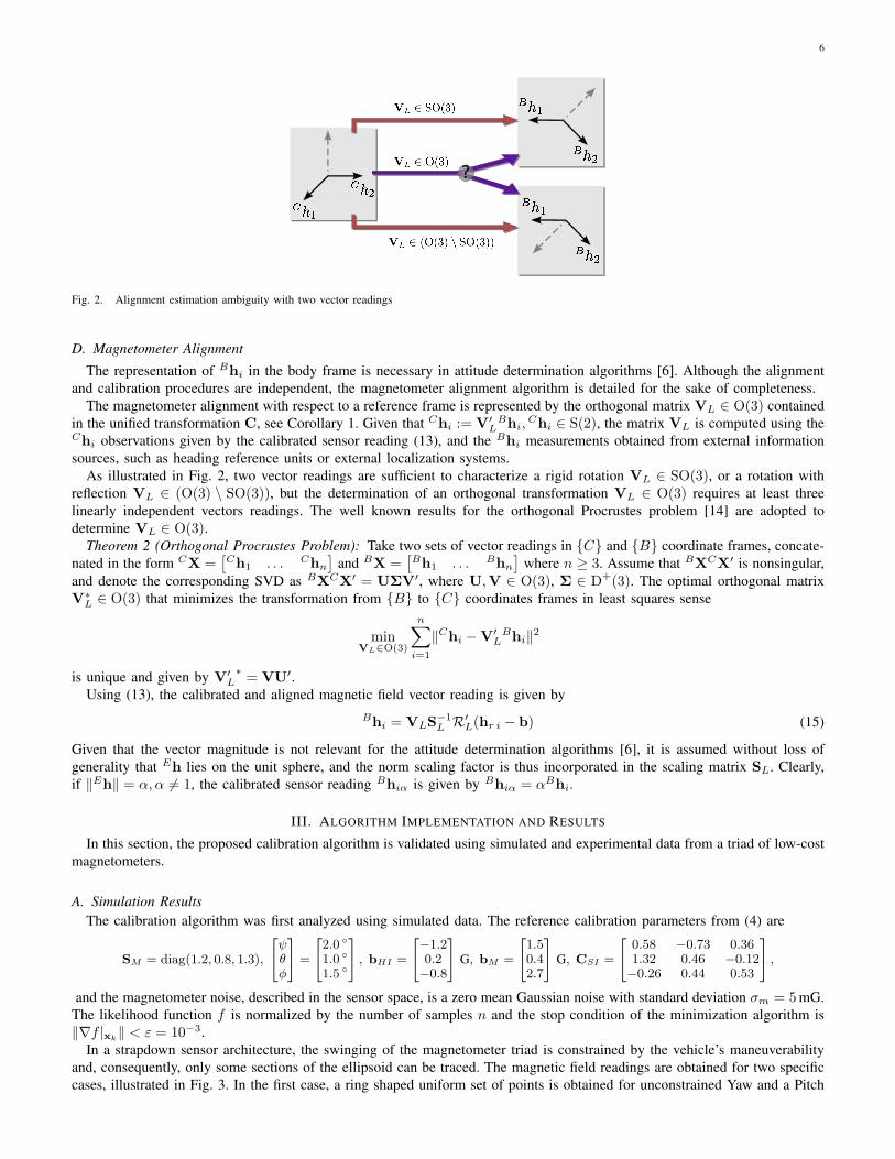
Fig. 2. Alignment estimation ambiguity with two vector readings

D. Magnetometer Alignment

The representation of Bhi in the body frame is necessary in attitude determination algorithms [6]. Although the alignment

and calibration procedures are independent, the magnetometer alignment algorithm is detailed for the sake of completeness.

The magnetometer alignment with respect to a reference frame is represented by the orthogonal matrix VL ∈ O(3) containedin the unified transformation C, see Corollary 1. Given that Chi := V′

LBhi,

Chi ∈ S(2), the matrix VL is computed using theChi observations given by the calibrated sensor reading (13), and the

Bhi measurements obtained from external information

sources, such as heading reference units or external localization systems.

As illustrated in Fig. 2, two vector readings are sufficient to characterize a rigid rotation VL ∈ SO(3), or a rotation withreflection VL ∈ (O(3) \ SO(3)), but the determination of an orthogonal transformation VL ∈ O(3) requires at least threelinearly independent vectors readings. The well known results for the orthogonal Procrustes problem [14] are adopted to

determine VL ∈ O(3).Theorem 2 (Orthogonal Procrustes Problem): Take two sets of vector readings in {C} and {B} coordinate frames, concate-

nated in the form CX =[

Ch1 . . . Chn

]

and BX =[

Bh1 . . . Bhn

]

where n ≥ 3. Assume that BXCX′ is nonsingular,

and denote the corresponding SVD as BXCX′ = UΣV′, where U,V ∈ O(3), Σ ∈ D+(3). The optimal orthogonal matrixV∗

L ∈ O(3) that minimizes the transformation from {B} to {C} coordinates frames in least squares sense

minVL∈O(3)

n∑

i=1

‖Chi − V′L

Bhi‖2

is unique and given by V′L∗

= VU′.

Using (13), the calibrated and aligned magnetic field vector reading is given by

Bhi = VLS−1L R′

L(hr i − b) (15)

Given that the vector magnitude is not relevant for the attitude determination algorithms [6], it is assumed without loss of

generality that Eh lies on the unit sphere, and the norm scaling factor is thus incorporated in the scaling matrix SL. Clearly,

if ‖Eh‖ = α, α 6= 1, the calibrated sensor reading Bhiα is given byBhiα = αBhi.

III. ALGORITHM IMPLEMENTATION AND RESULTS

In this section, the proposed calibration algorithm is validated using simulated and experimental data from a triad of low-cost

magnetometers.

A. Simulation Results

The calibration algorithm was first analyzed using simulated data. The reference calibration parameters from (4) are

SM = diag(1.2, 0.8, 1.3),

[

ψθφ

]

=

[

2.0 ◦

1.0 ◦

1.5 ◦

]

, bHI =

[

−1.20.2−0.8

]

G, bM =

[

1.50.42.7

]

G, CSI =

[

0.58 −0.73 0.361.32 0.46 −0.12−0.26 0.44 0.53

]

,

and the magnetometer noise, described in the sensor space, is a zero mean Gaussian noise with standard deviation σm = 5mG.The likelihood function f is normalized by the number of samples n and the stop condition of the minimization algorithm is

‖∇f |xk‖ < ε = 10−3.

In a strapdown sensor architecture, the swinging of the magnetometer triad is constrained by the vehicle’s maneuverability

and, consequently, only some sections of the ellipsoid can be traced. The magnetic field readings are obtained for two specific

cases, illustrated in Fig. 3. In the first case, a ring shaped uniform set of points is obtained for unconstrained Yaw and a Pitch

7

(a) Ring Shaped Data (b) Arch Shaped Data

Fig. 3. Ellipsoid fitting (Simulation Data)

sweep interval of θ ∈ [−20, 20] ◦. Note that the constraint in the Pitch angle can be found in most terrestrial vehicles. In thesecond case, the ellipsoid’s curvature information is reduced by constraining the Yaw to ψ ∈ [−90, 90] ◦.The results of 20 Monte Carlo simulations using 104 magnetometer readings are presented in Tables I and II and depicted

in Fig. 3. Given the large likelihood cost of the noncalibrated data, denoted by f(x−1), the initial condition draws the costfunction into the vicinity of the optimum, and the iterations yield a 20% improvement over the initial guess.

TABLE ICALIBRATION RESULTS (GRADIENT METHOD)

f(x−1) f(x0) f(x∗) iterations θe se be

Ring Shaped Data 3.28 × 10−1 1.17 × 10−4 9.64 × 10−5 2246 1.74 × 10−3 7.61 × 10−3 3.54 × 10−4

Arch Shaped Data 4.36 × 10−1 1.18 × 10−4 9.62 × 10−5 1932 1.46 × 10−2 1.65 × 10−2 1.74 × 10−2

TABLE IICALIBRATION RESULTS (NEWTON METHOD)

f(x−1) f(x0) f(x∗) iterations θe se be

Ring Shaped Data 3.28 × 10−1 1.18 × 10−4 9.64 × 10−5 37.0 1.74 × 10−3 7.61 × 10−3 3.54 × 10−4

Arch Shaped Data 4.37 × 10−1 1.18 × 10−4 9.62 × 10−5 37.2 1.46 × 10−2 1.65 × 10−2 1.75 × 10−2

The Newton algorithm converges faster than the gradient algorithm, exploiting the second order information of the Hessian,

as illustrated in Fig. 4 and Fig. 5. Although the Hessian computations are more complex, the Newton method takes only 5 sto converge to in a Matlab 7.3 implementation running on a standard computer with a Pentium Celeron 1.6 Ghz processor.Defining the distance between the estimated and the actual parameter as se := ‖S∗ − S‖,be := ‖b∗ − b‖, and θe :=

arccos(

tr(R∗R′)−12

)

, Tables I and II show that the arch shaped data set contains sufficient eccentricity information to estimate

the equivalent magnetometer errors quantitiesR, s and b. For platforms with limited maneuverability, the proposed optimization

algorithm identifies the calibration parameters with good accuracy. As expected, reducing the information about the ellipsoid

curvature slightly degrades the sensor calibration errors.

As depicted in Fig. 3, although the noise is formulated in the sensor frame, the suboptimal formulation (10) yields accurate

results with unitary likelihood weights σ2m i. Let the distance in the parameter space be given by d(x

∗,x)2 := θ2e + s2e + b2

e,

the influence of the noise power in the estimation error is illustrated in Fig. 6, where the magnetic field magnitude in the San

Francisco Bay area is adopted, ‖Eh‖ = 0.5G.

B. Experimental Results

The algorithm proposed in this work was used to estimate the calibration parameters for a set of 6 × 104 points obtained

from an actual magnetometer triad. The magnetometer was a Honeywell HMC1042L 2-axis magnetometer and a Honeywell

HMC1041Z for the third (Z) axis, sampled with a TI MSC12xx microcontroller with a 24bit Delta Sigma converter, at 100Hz,

see [10] for details.

8

0 5 10 15 20 25 30 350.00009

0.0001

0.00011

0.00012

iteration

f(x

k)

Newton Method

Gradient Method

(a) Newton (vs Gradient) Method

0 500 1000 15000.00009

0.0001

0.00011

0.00012

iteration

f(x

k)

(b) Gradient Method Iterations

Fig. 4. Convergence of the Log-Likelihood Function (Arch Shaped Data)

0 5 10 15 20 25 30 3510

−3

10−2

10−1

100

101

102

iteration

||∇

f| x

k||

Newton Method

Gradient Method

(a) Newton (vs Gradient) Method

0 500 1000 150010

−3

10−2

10−1

100

101

102

iteration

||∇

f| x

k||

(b) Gradient Method Iterations

Fig. 5. Convergence of the Log-Likelihood Gradient (Arch Shaped Data)

103

104

105

106

10−7

10−6

10−5

10−4

10−3

10−2

SNR( ||Eh ||2 /σ2m

)

d(x∗

,x)

2

Simulated SNR

Experimental SNR

Fig. 6. Estimation Error vs. Signal-to-Noise Ratio (100 MC, Ring Shaped Data)

9

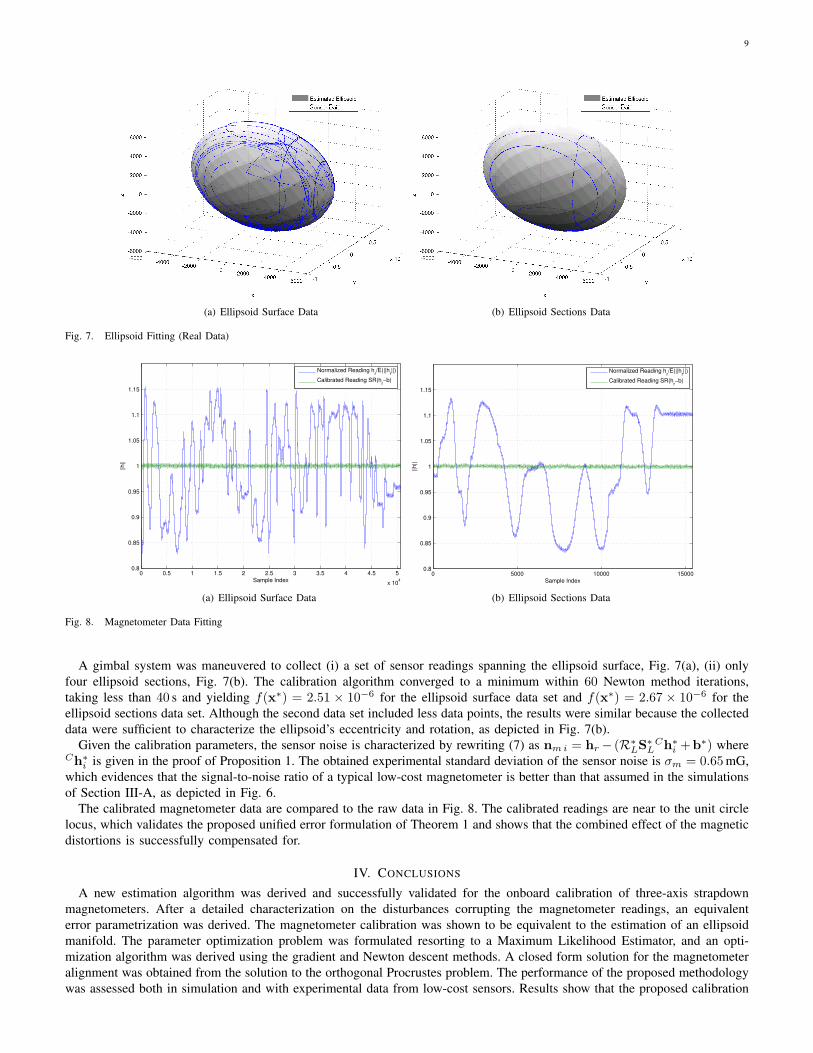
(a) Ellipsoid Surface Data (b) Ellipsoid Sections Data

Fig. 7. Ellipsoid Fitting (Real Data)

0 0.5 1 1.5 2 2.5 3 3.5 4 4.5 5

x 104

0.8

0.85

0.9

0.95

1

1.05

1.1

1.15

||h

||

Sample Index

Normalized Reading h

r/E(||h

r||)

Calibrated Reading SR(hr−b)

(a) Ellipsoid Surface Data

0 5000 10000 150000.8

0.85

0.9

0.95

1

1.05

1.1

1.15

||h

||

Sample Index

Normalized Reading h

r/E(||h

r||)

Calibrated Reading SR(hr−b)

(b) Ellipsoid Sections Data

Fig. 8. Magnetometer Data Fitting

A gimbal system was maneuvered to collect (i) a set of sensor readings spanning the ellipsoid surface, Fig. 7(a), (ii) only

four ellipsoid sections, Fig. 7(b). The calibration algorithm converged to a minimum within 60 Newton method iterations,taking less than 40 s and yielding f(x∗) = 2.51 × 10−6 for the ellipsoid surface data set and f(x∗) = 2.67 × 10−6 for the

ellipsoid sections data set. Although the second data set included less data points, the results were similar because the collected

data were sufficient to characterize the ellipsoid’s eccentricity and rotation, as depicted in Fig. 7(b).

Given the calibration parameters, the sensor noise is characterized by rewriting (7) as nm i = hr − (R∗LS∗

LCh∗

i +b∗) whereCh∗

i is given in the proof of Proposition 1. The obtained experimental standard deviation of the sensor noise is σm = 0.65mG,which evidences that the signal-to-noise ratio of a typical low-cost magnetometer is better than that assumed in the simulations

of Section III-A, as depicted in Fig. 6.

The calibrated magnetometer data are compared to the raw data in Fig. 8. The calibrated readings are near to the unit circle

locus, which validates the proposed unified error formulation of Theorem 1 and shows that the combined effect of the magnetic

distortions is successfully compensated for.

IV. CONCLUSIONS

A new estimation algorithm was derived and successfully validated for the onboard calibration of three-axis strapdown

magnetometers. After a detailed characterization on the disturbances corrupting the magnetometer readings, an equivalent

error parametrization was derived. The magnetometer calibration was shown to be equivalent to the estimation of an ellipsoid

manifold. The parameter optimization problem was formulated resorting to a Maximum Likelihood Estimator, and an opti-

mization algorithm was derived using the gradient and Newton descent methods. A closed form solution for the magnetometer

alignment was obtained from the solution to the orthogonal Procrustes problem. The performance of the proposed methodology

was assessed both in simulation and with experimental data from low-cost sensors. Results show that the proposed calibration

10

algorithm can be adopted for a wide variety of autonomous vehicles with maneuverability constraints and in situations that

require periodic onboard sensor calibration. Future work will include the adaptation of the proposed algorithm to the 2D

(heading only) case in marine and land robotics.

EXTERNAL MAGNETIC NOISE

In the proposed error model (4), electronic interference and sensor specific technology are the main sources of noise. In the

case where the main sources of electromagnetic interference are external, the magnetic noise influence in the magnetometer

reading can be modeled as

hr i = SMCNO(CSI(BERi

Eh + BNRnm i) + bHI) + bM = CBhi + CB

NRnm i + b

= RLSLChi + RLSLV′

LBNRnm i + b (16)

where BNR rotates from the coordinate frame {N} where the magnetic noise is defined, to the body coordinate frame. Assuming

that nm i is a zero mean Gaussian process with variance σ2m i, the p.d.f. of each hr i is also Gaussian

nm i ∼ N (0, σ2

m iI) ⇒ hr i ∼ N (RLSLChi + b, σ

2

m iRLS2

LR′

L).

Using the p.d.f. of the hr i, straightforward analytical derivations show that MLE formulation is given by (9). As convincingly

argued in [22], if the noise exists in the sensor frame (7), the ellipsoid obtained by (9) tends to fit best the points with lower

eccentricity. This effect can be balanced by defining appropriate curvature weights [22] σ2m i, producing results close to the

optimal solution of (8).

LIKELIHOOD FUNCTION DERIVATIVES

Let ui := hr i − b, the gradient of the likelihood function

f :=

n∑

i=1

(

‖T(hr i − b)‖ − 1

σm i

)2

,

denoted by ∇f |x =[

∇f |T ∇f |b]

, is described by the submatrices

∇f |T =n∑

i=1

2cTσ2

m i

ui ⊗ Tui, ∇f |b =n∑

i=1

−2cTσ2

m i

T′Tui,

where cT := 1 − ‖Tui‖−1and ⊗ denotes the Kronecker product [23]. The Hessian ∇2f |x =

[

HT,T HT,b

H′

T,b Hb,b

]

is given by the

following submatrices

HT,T =

n∑

i=1

2

σ2

m i

[

(uiu′

i) ⊗ (Tuiu′

iT′)

‖Tui‖3+ cT

[

(uiu′

i) ⊗ I]

]

, HT,b =

n∑

i=1

−2

σ2

m i

[

(ui ⊗ Tui)u′

iT′T

‖Tui‖3+ cT (ui ⊗ T + I ⊗ Tui)

]

Hb,b =

n∑

i=1

2

σ2

m i

[

T′Tuiu

′

iT′T

‖Tui‖3+ cT T

′

T

]

.

ACKNOWLEDGMENTS

This work was partially supported by Fundacao para a Ciencia e a Tecnologia (ISR/IST plurianual funding) through the

POS Conhecimento Program that includes FEDER funds and by the project MEDIRES from ADI and project PDCT/MAR/55609/2004

- RUMOS of the FCT. The work of J.F. Vasconcelos was supported by a PhD Student Scholarship, SFRH/BD/18954/2004,

from the Portuguese FCT POCTI programme.

REFERENCES

[1] T. E. Humphreys, M. L. Psiaki, E. M. Klatt, S. P. Powell, and P. M. Kintner, Jr., “Magnetometer-based attitude and rate estimation for spacecraft withwire booms,” Journal of Guidance, Control, and Dynamics, vol. 28, no. 4, pp. 584–593, July-August 2005.

[2] D. Choukroun, I. Y. Bar-Itzhack, and Y. Oshman, “Optimal-request algorithm for attitude determination,” Journal of Guidance, Control, and Dynamics,vol. 27, no. 3, pp. 418–425, May-June 2004.

[3] I. Bar-Itzhack and R. Harman, “Optimized TRIAD Algorithm for Attitude Determination,” Journal of Guidance, Control, and Dynamics, vol. 20, no. 1,pp. 208–211, 1997.

[4] D. M. F. L. Markley, “Quaternion attitude estimation using vector observations,” Journal of Astronautical Sciences, vol. 48, no. 2, pp. 359–380, 2000.[5] NOAA Technical Report: The US/UK World Magnetic Model for 2005-2010, National Oceanic and Atmospheric Administration, U.S. Department ofCommerce, 2004.

[6] F. Markley, “Attitude determination and parameter estimation using vector observations: Theory,” The Journal of the Astronautical Sciences, vol. 37,no. 1, pp. 41–58, January-March 1989.

[7] W. Denne, Magnetic Compass Deviation and Correction, 3rd ed. Sheridan House Inc, 1979.[8] N. Bowditch, The American Pratical Navigator, Hydrographic/Topographic Center, Defense Mapping Agency, 1984.

11

[9] D. Gebre-Egziabher, G. Elkaim, J. Powell, and B. Parkinson, “Calibration of Strapdown Magnetometers in Magnetic Field Domain,” ASCE Journal ofAerospace Engineering, vol. 19, no. 2, pp. 1–16, April 2006.

[10] G. Elkaim and C. Foster, “Development of the metasensor: A low-cost attitude heading reference system for use in autonomous vehicles,” in Proceedingsof the ION Global Navigation Satellite Systems Conference (ION-GNSS 2006), Fort Worth, TX, USA, September 2006.

[11] R. Alonso and M. Shuster, “Complete linear attitude-independent magnetometer calibration,” The Journal of the Astronautical Sciences, vol. 50, no. 4,pp. 477–490, October-December 2002.

[12] B. Gambhir, “Determination of Magnetometer Biases Using Module RESIDG,” Computer Sciences Corporation, Tech. Rep. 3000-32700-01TN, March1975.

[13] J. Crassidis, K. Lai, and R. Harman, “Real-time attitude-independent three-axis magnetometer calibration,” Journal of Guidance, Control, and Dynamics,vol. 28, no. 1, pp. 115–120, January-February 2005.

[14] J. C. Gower and G. B. Dijksterhuis, Procrustes Problems, ser. Oxford Statistical Science Series. Oxford University Press, USA, 2004, no. 30.[15] G. Elkaim and C. Foster, “Extension of a Non-Linear, Two-Step Calibration Methodology to Include Non-Orthogonal Sensor Axes,” 2006, iEEE Journal

of Aerospace Electronic Systems, Technical Note, submitted August 2006, accepted for publication.[16] G. Strang, Linear Algebra and Its Applications, 3rd ed. Brooks Cole, 1988.[17] A. Edelman, T. Arias, and S. Smith, “The geometry of algorithms with orthogonality constraints,” SIAM Journal on Matrix Analysis and Applications,

vol. 20, no. 2, pp. 303–353, 1998.[18] D. Gabay, “Minimizing a differentiable function over a differential manifold,” Journal of Optimization Theory and Applications, vol. 37, no. 2, pp.

177–219, June 1982, communicated by D.G. Luenberger.[19] S. Kay, Fundamentals of Statistical Signal Processing: Estimation. Upper Saddle River, New Jersey, USA: Prentice-Hall, 1993.[20] D. Bertsekas, Nonlinear Programming, 2nd ed. Athena Scientific, 1999.[21] G. Calafiore, “Approximation of n-dimensional data using spherical and ellipsoidal primitives,” IEEE Transactions on Systems, Man and Cybernetics -

Part A: Systems and Humans, vol. 32, no. 2, pp. 269–278, March 2002.[22] W. Gander, G. Golub, and R. Strebel, “Least-squares fitting of circles and ellipses,” BIT, vol. 43, pp. 558–578, 1994.[23] H. Lutkepohl, Handbook of Matrices. John Wiley & Sons, 1997.