1 9 APR 2000

Development of Numerical Constitutive Models for Carbon-Carbon Composites F49620-94-l-0259,P00002

John Whitcomb

Center for Mechanics of Composites Texas A & M University

tFinalRepoit May 15, 1994 - August 31, 1998

Objective Predict the stiffness and strength of oxidation-resistant carbon-carbon subjected to thermal

and mechanical loads in an oxidizing environment

Status of effort A three-dimensional progressive failure analysis of carbon-carbon composites was

developed. To facilitate the study, various mesh generators and graphical pre- and post- processing tools were developed. These tools were used to study carbon-carbon during cool- down from processing temperature and subsequent mechanical loads. This grant was tightly integrated with the AASERT grant F49620-93-1-0471, which ended last year. The student supported under the AASERT grant, Clint Chapman, has graduated (and is employed) with a Ph.D. This final year of the subject grant has been invested in documenting our efforts in the open literature and assembling documentation for the tools developed by Dr. Chapman so they could be used in subsequent projects.

Accomplishments Two of the biggest challenges in the analysis of textile composites is developing a valid 3D

finite element mesh and deriving boundary conditions for the smallest possible analysis region (since the computational challenge is inherently high). We can now obtain meshes and boundary conditions for plain and 8 harness satin weaves with a wide range of waviness, tow cross-section, and mesh refinement. Only a few parameters have to be specified.. .the rest is automatic. We have also enhanced our visualization programs and associated utilities so that it is much more convenient to examine stress and strain distributions, deformed geometries, damage distribution, and differences between models.

We have continued to document our efforts in the literature. The results of our simulations were presented at ICCE/5 in July, 1998. A journal paper describing the simulations is almost complete. The title is "Thermally Induced Damage Initiation and Growth in Carbon- Carbon Composites." Another paper, "Derivation of Boundary Conditions for Micromechanics Analyses of Plain and Satin Weave Composites," has already been submitted to the Journal of Composite Materials. The new techniques developed in this paper greatly simplify the challenge of deriving boundary conditions. Reports from previous years of this grant include coüies of

DKC QUALITY EJePECUD 4 ___«.MJA J 4 A

20000710 119

REPORT DOCUMENTATION PAGE

Public reporting burden for this collection of information is estimated to average 1 hour per response, including the time for reviewing instructions, searcl the collection of information. Send comments regarding this burden estimate or any other aspect of this collection of information, including sugges Operations and Reports, 1215 Jefferson Davis Highway, Suite 1204, Arlington, VA 222024302, and to the Offic». of Management and Budget, Paper»

1. AGENCY USE ONLY (Leave blank) 2. REPORT DATE 3. REPOR",

AFRL-SR-BL-TR-OO- ewmg nation

Final Technical Report 14 May 94 - 31 Auf 98 4. TITLE AND SUBTITLE

(U) DEVELOPMENT OF NUMERICAL CONSTITUTIVE MODELS FOR CARBON-CARBON COMPOSITES

6. AUTHOR(S)

JOHN WHITCOMB

5. FUNDING NUMBERS

F49620-94-1-0259

2302/BS 61102F

7. PERFORMING ORGANIZATION NAME(S) AND ADDRESS(ES)

TEXAS A&M UNIVERSITY CENTER FOR MECHANICS OF COMPOSITES COLLEGE STATION, TX 77843

8. PERFORMING ORGANIZATION REPORT NUMBER

9. SPONSORING/MONITORING AGENCY NAME(S) AND ADDRESS(ES)

AIR FORCE OFFICE OF SCIENTIFIC RESEARCH AEROSPACE AND MATERIALS SCIENCES DIRECTORATE 801 N. RANDOLPH STREET, ROOM 732 ARLINGTON, VA 22203-1977

10. SPONSORING/MONITORING AGENCY REPORT NUMBER

11. SUPPLEMENTARY NOTES

12a. DISTRIBUTION AVAILABILITY STATEMENT

APPROVED FOR PUBLIC RELEASE DISTRIBUTION IS UNLIMITED

12b. DISTRIBUTION CODE

13. ABSTRACT {Maximum 200 words) A three-dimensional progressive failure analysis of carbon-carbon composites was developed. To facilitate the study, various mesh generators and graphical pre- and post-processing tools were developed. These tools were used to study carbon-carbon during cool-down from processing temperature and subsequent mechanical loads. This grant was tightly integrated with the AASERT grant F49620-93-1-0471, which ended last year. The student supported under the AASERT grant, Clint Chapman, has graduated (and is employed) with a Ph.D. This final year of the subject grant has been invested in documenting our efforts in the open literature and assembling documentation for the tools developed by Dr. Champan so they could be used in subsequent projects.

14. SUBJECT TERMS 15. NUMBER OF PAGES

28 16. PRICE CODE

17. SECURITY CLASSIFICATION OF REPORT

UNCLASSIFIED

18. SECURITY CLASSIFICATION OF THIS PAGE

UNCLASSIFIED

19. SECURITY CLASSIFICATION OF ABSTRACT

UNCLASSIFIED

20. LIMITATION OF ABSTRACT

Standard Form 298 (Rev. 2-89) (EG) Prescribed by ANSI Std. 230.18 Designed using Perform Pro, WHS/DIOR, Oct 94

papers and Clint's PhD dissertation, so they will not be included herein. Attached is a copy of the paper "Derivation of Boundary Conditions for Micromechanics Analyses of Plain and Satin Weave Composites," which has been submitted. When other papers are ready for submission to a journal, they will be forwarded to the technical monitor.

Peer Reviewed Publications 1. Whitcomb, J.D.; Chapman, C: Effect of Assumed Tow Architecture and Mesh Refinement

on the Predicted Moduli and Stresses in Plain Weave Composites. Journal of Composite Materials. Vol. 29, No. 16, pp. 2134-2159, 1995.

2. Whitcomb, J.D.; Srirengan, K.; Chapman, C: Evaluation of Homogenization for Global/Local Stress Analysis of Textile Composites. Composite Structures. Vol. 31, No. 2, pp. 137-149, 1995.

3. Whitcomb, J.D.; Chapman, C: Analysis of Plain Weave Composites Subjected to Flexure. Mechanics of Composite Materials and Structures. Vol. 5, No. 1, pp. 41-53, 1998.

4. Srirengan, K.; Whitcomb, J.D.; Chapman, C: Modal Technique for Three-Dimensional Stress Analysis of Plain Weave Composites. Composite Structures. Vol. 39, NO. 1-2, pp. 145- 156, 1997.

5. Whitcomb, J.D.; Chapman, CD., Tang, X.: Derivation of Boundary Conditions for Micromechanics Analyses of Plain and Satin Weave Composites. Submitted 8/98 to Journal of Composite Materials.

6. Chapman, CD.; Whitcomb, J.D.: Thermally Induced Damage Initiation and Growth in Carbon-Carbon Composites (manuscript in preparation).

Conference and Workshop Presentations

1. Whitcomb, J.D.; Srirengan, K.; and Chapman, C: Evaluation of Homogenization for Global/Local Stress Analysis of Textile Composites. Presented at the AIAA/ASME/ASCE/AHS/ASC 35th Structures, Structural Dynamics, and Materials conference, Hilton Head, South Carolina, April 18-20, 1994.

2. Whitcomb, J.D.; Srirengan, K.; and Chapman, C: Simulation of Progressive Failure in Plain Weave Textile Composites. Presented at 1994 ASME Winter Annual Meeting, Chicago, Illinois, November 13-18, 1994.

3. Chapman, C; Whitcomb, J.D.; and Srirengan, K.: Analysis of Woven Composites Subjected to Flexure. Society of Engineering Science 31st Annual Technical Meeting, College Station, Texas, October 10-12, 1994.

4. Srirengan, K.; Whitcomb, J.D.; and Chapman, C: Three-Dimensional Analysis of Woven Composites Subjected to Flexure. Third U.S. National Congress of Computational Mechanics, June 12-14, 1995.

5. Chapman, C; and Whitcomb, J.D.: Thermomechanical Characterization of Plain and Satin Weave Carbon-Carbon Composites. Third U.S. National Congress of Computational Mechanics, June 12-14, 1995.

6. Whitcomb, J.D.; Srirengan, K; and Chapman, C: Modal Technique for Three Dimensional Stress Analysis of Plain Weave Composites. ICCM-10, Whistler, Canada, August 14-29. 1995.

7. Chapman, C; and Whitcomb, J.D.: Strategy for Modeling Eight-Harness Satin Weave Carbon/Carbon Composites Subjected to Thermal Loads. Presented at 37th AIAA/ASME/ASCE/AHS/ASC Structures, Structural Dynamics, and Materials Conference, Salt Lake City, UT, April 15-17, 1996.

8. Whitcomb, J.D.; and Chapman, C: Thermally Induced Damage Initiation and Growth in Carbon-Carbon Composites. Presented at the 38th AIAA/ASME/ASCE/AHS/ASC Structures, Structural Dynamics, and Materials Conference, Kissimmee, FL, April 7-10, 1997.

9. Whitcomb, J.D.; and Chapman, C: Damage Initiation and Growth in Carbon-Carbon Composites Subjected to Thermal and Mechanical Loads. Presented at the 1997 Joint ASME/ASEE/SES Summer Meeting, Chicago, IL, June 28- July 2, 1997.

10. Whitcomb, J.D.; Tang, X.; and Chapman, C: Simulation of Progressive Failure of Woven Composites Engineering, to be presented at ICCE/5 Fifth International Conference on Composites Engineering, Las Vegas, NV, July 5-11, 1998.

11. Whitcomb, J.D.; Tang, X.; and Chapman, C: Comparison of Stress Concentrations in Plain and Satin Weave Composites, to be presented at the International Mechanical Engineering Congress and Exposition, Dallas, TX, Nov. 1998.

* *

8/19/98 - C:\whit_Rest\Papers\BC_forWeave\weaveBC_l .doc 1

Derivation of Boundary Conditions for Micromechanics Analyses of Plain and Satin Weave

Composites

John D. Whitcomb

Clinton D. Chapman

XiaodongTang

Abstract

Efficient 3D analysis of periodic structures depends on identifying the smallest region to

be modeled and the appropriate boundary conditions. This paper describes systematic procedures

for deriving the boundary conditions for general periodic structures. These procedures are then

used to derive the boundary conditions for plain and satin weave composites.

Introduction

Composite materials consist of a combination of materials, often fibers and matrix. The

basic challenge of micromechanics is to determine how the properties and spatial distribution of

the constituents affect the overall material response. The overall response is often characterized

in terms of the effective engineering properties, such as extensional moduli and Poisson's ratio.

These are also referred to as the homogenized engineering properties. To obtain these properties

a representative volume element (RVE) or unit cell is identified that includes all characteristics

of the composite. The literature includes a wide variety of analyses for various unit cells. For

example, some of the recent numerical studies have focused on hexagonal and square arrays of

fibers in matrix [1-4], spherical inclusions in matrix [5], and textile composites [6-13]. The latter

configuration, textile composites, presents a severe challenge to the analyst because of the

geometric complexity. Although a variety of analyses exist, including some very detailed three-

dimensional finite element analyses [7-13], there has not been a systematic description of how

one obtains the boundary conditions to perform the analysis of textile composites. Reference [14]

gives an excellent discussion of exploiting symmetry in general. However, the reference does

not consider periodicity explicitly or composites. Accordingly, the goal of this paper is to present

a systematic procedure for deriving the boundary conditions for both full unit cell and partial unit

cell analyses of plain and satin weave composites.

*<

8/19/98 - C:\whit_Rest\Papers\BC_forWeave\weaveBC_l.doc 2

Background

Implicit in micromechanics analyses is that a small region of the microstructure fully

represents the behavior of a much larger region (usually an infinite domain). There is no standard

definition of this region in the literature. Herein, the term "unit cell" is defined to mean the

smallest region that represents the behavior of the larger region without any mirroring or rotation

transformations. For such a region to exist there must be a basic pattern (of geometry and

response, such as strains, stresses, etc.) that is repeated periodically throughout a domain. In

particular, the larger region can be synthesized by replication and translation of the unit cell in

the three coordinate directions. Figure 1 shows examples of periodic microstructure. In each

case, the region is built from a single building block or unit cell. Note that there can be more than

one definition of the unit cell for a single microstructure (e.g. case (a) in Figure 1).

To determine effective engineering properties, the periodic array is subjected to a series

of loads consisting of either macroscopically constant strain or stress. The term macroscopically

constant indicates that the volume averaged strain for every unit cell is identical. (The same can

be said for the stresses.) Although one cannot analyze an infinite number of unit cells, it is

possible to derive boundary conditions for a single unit cell that will make it behave as though it

is buried within an infinite array. How this is done will be described herein.

It is convenient to think of the challenge as consisting of two parts. The first part consists

of identifying the appropriate boundary conditions for a single full unit cell. The second

challenge is to exploit the symmetries in the microstructure of the unit cell and the loading to

reduce the analysis region to just a fraction of the full cell in order to reduce the computational

costs.

Derivation of basic equations

The derivation of the boundary conditions is based on two conditions. The first is

periodicity and the second is equivalence of coordinate system. It should be noted that that these

concepts can be combined, but the authors choose not to do so. The periodic conditions state

that the displacements in the various unit cells differ only by constant offsets that- depend on the

U

8/19/98 - C:\whit_Rest\PapersVBC_forWeave\weaveBC_l .doc 3

volume averaged displacement gradients/Further, the strains and stresses are identical in all of

the unit cells. This can be expressed as

*,(*.+*.) «*»(*.) (1)

where dß is a vector of periodicity. This vector is a vector from a point in one unit cell to an

equivalent point in another unit cell.

These conditions are sufficient for deriving the boundary conditions for the full unit cell.

However, it is usually desirable to exploit symmetries in order to be able to analyze a smaller

region. The concept of "Equivalent Coordinate Systems" (ECS) is useful in identifying the

symmetries and constraint conditions. Coordinate systems are equivalent if the geometry, spatial

distribution of material, loading, and the various fields that describe the response (e.g.

displacement, strains, etc.) are identical in the two systems.

For example, xt and xt are equivalent coordinate systems if

**(*«) = **(*«)

*,(*.) ^(»J (2)

etc.

A visual technique for determining whether a new coordinate system is equivalent is to draw it

on a three-dimensional view of the body. This view should include the load vectors and a

description of the spatial variation of the material properties. If the body can be rotated (i.e. the

view changed) such that the new view and new coordinate system look identical to the original

view and coordinate system, the coordinate system is equivalent.

Exploiting equivalent coordinate systems requires identification of coordinate transformations

that provide useful constraint conditions. Consider the equivalent coordinate system x. as a

H

8/19/98 - C:\whit_Rest\Papefs\BC_forWeave\weaveBC_l.dcx: 4

potentially useful ECS. Define: a& = direction cosines for transformation from the original (x,)

to the equivalent (*,) coordinate system....i.e. xt = atj xt

**(*«) = ^V«(*«) (3) 5vfe) = «i««/H<r«(S«)

Combine equations (2) and (3) to give

«,(*«) = «*«/(*«) ^{xa) = aimaJnsim(xa) (4)

^iJM = aimajnaJxa)

Finally, replace xa with aaj Xj so that everything is now expressed in terms of a single

coordinate system.

^{xa) = aima.nsJa^X]) (5)

Sometimes it is necessary to switch the sign of all of the loads to make the two coordinate

systems equivalent. If tension and compression properties are different, one must not switch the

sign of the load to obtain an equivalent coordinate system.

To generalize equations (5), a factor y is introduced.

y = 1 if load reversal is not required

y = -1 if load reversal is required

Equation (5) then becomes

^M-ro^a^eJa^Xj) (6)

"»(*«) = 7 <V^«K XJ)

U

8/19/98 - C:\whit_Rest\Papers\BC_forWeave\weaveBC_l.doc 5

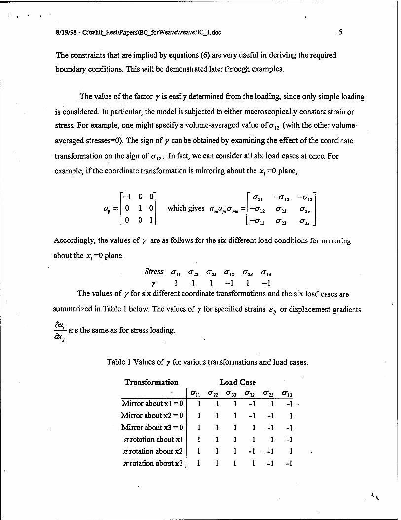
The constraints that are implied by equations (6) are very useful in deriving the required

boundary conditions. This will be demonstrated later through examples.

The value of the factor y is easily determined from the loading, since only simple loading

is considered. In particular, the model is subjected to either macroscopically constant strain or

stress. For example, one might specify a volume-averaged value of <Jn (with the other volume-

averaged stresses=0). The sign of y can be obtained by examining the effect of the coordinate

transformation on the sign of an. In fact, we can consider all six load cases at once. For

example, if the coordinate transformation is mirroring about the xx =0 plane,

aü =

"-1 0 0* 0 1 0 0 0 1

which gives aji^a^- '12

-o-, 13

-°"l2 -°"l3 CT22 0"23

Ö-23 CT33.

Accordingly, the values of y are as follows for the six different load conditions for mirroring

about the xx =0 plane.

Stress au cr22 cr33 al2 a^ al3

y 111-11-1 The values of y for six different coordinate transformations and the six load cases are

summarized in Table 1 below. The values of y for specified strains etj or displacement gradients

du, dx

- are the same as for stress loading.

Table 1 Values of y for various transformations and load cases.

Transformation Load Case o"n CT22 O» <T,2 Ö-23 013

Mirror about xl = 0 11-11 -1 Mirror about x2 = 0 1 1-1-1 Mirror about x3 = 0 111-1 -1

^rotation about xl 11-11 -1

/notation about x2 1 1 -1-1 ^rotation about x3 111-1 -1

8/19/98-C:\whit_Rest\Papers\BC_forWeave\weaveBC_l.doc 6

The values of y also indicate what types of loading can exist for a particular type of equivalent coordinate system. For example, for mirroring about the xx axis one cannot impose non-zero volume averaged values of both su and sn at the same time ... the symmetries are incompatible since they require different values of y. Furthermore, if one imposes a non-

zero (en) and retains the other strains as unknowns to be determined as part of the solution,

(fi-,2) and (e 13)must be found to be zero.

Boundary conditions for symmetrically stacked plain weave

If one is willing to analyze the entire unit cell, the periodic conditions for the

displacements can be used to specify the boundary conditions. However, to reduce the region to

be analyzed requires a bit more effort. The following describes a systematic way to go about

accomplishing this task. Although the focus is on the plain weave, the techniques are quite

general. Figure 2a is a unit cell for a symmetrically stacked plain weave composite. As can be

seen from the figure, the planes x( = 0 are planes of geometric symmetry.

The first step will be to develop relationships for the planes xx = ±a. (vector of periodicity

da =[2a,0,0]) Substituting Xj = -a into the periodic relations gives

ut {a, x2, x3 ) = w, (-a, x2,x3) + {^T/2a

Sy (a, x2ix3) = etj (-a, x2 ,x3) . (7)

cTtj(a, x2, x3) = cXiji-a, x2,x3)

Consider the equivalent coordinate system (ECS) xa that is obtained by mirroring about xx = 0.

The direction cosines for this transformation are

"-1 0 0'

0 1 0

0 0 1 atf= 0 10 (8)

Substituting the atj above into equations (6) yields the following relationships for displacements

and stresses,

H

8/19/98 - C:\whit_Rest\PapcrS\BC_forWeave\weaveBC_l.doc

'li

'12

»13

V ""V U2 -Y u2

W Ca^iJfi) .wsJ {-eJCiJCy)

Ö-J2 °"l3 °H _0"l2 -0"I3

a22 °23 = -0-J2 cr22 °23

°"23 °"33. (fl^r2^3) -<Jn OK o-33

(9)

(-a^2 ^3)

Tractions will transform like the displacements and strains like the stresses, so the details are not

shown. These periodic and ECS conditions will now be combined ... first for displacements and

then for the stresses.

Displacements

Combining the constraints in equations (7) and (9) yields:

\dxt

du2

Rearranging, yields

u.

«<>

LM3J (-a,x2,x3) [dx1

1&U

u2(i-y) u3(i-r\

2a = y -ih

U*

u-.

(-a,x2,x3)

(-a,x2,x3)

'du2 la

(10)

(11)

Recall that the value of y depends on whether the loads must be reversed for the new coordinate

system to be equivalent. The constraints indicated by equation (11) are listed below. The ones

that provide useful information are boxed. The remaining constraints are not useful for

performing the analysis, but they can be used for evaluating the results.

8/19/98 - C:\whit_Rest\Papcrs\BC_forWeave\weaveBC_l.doc

r = i

<du2

A, = 0

r=-\

{dxj

u2{-a,x2,x3) = -{-^-\a

u3(-a,x2,x3) = -&)a

(12)

This can be expressed quite succinctly as follows

• If y — 1, normal displacements on xx = -a are equal. Because of periodicity, the normal

displacements on xx = a are also equal and opposite those onxj = -a.

• If Y = -1, tangential displacements are constant in each direction on xx = -a. Because of

periodicity, the tangential displacements in each direction on xy = a are also equal and

opposite the corresponding displacements on xx = -a.

Stresses

Now consider the constraints on the stresses. Combine equations (7) and (9) to obtain the

following useful relations (the remainder are trivially satisfied or do not affect the boundary

conditions.)

Y = V. crl2{±a,x2,x3) = 0

Y = -l: an(±a,x2,x3) = 0

crl3(±asx2,x3) = 0 (13)

These can be summarized as follows (using Cauchy's stress formula, xt = crfinj)

• If Y — 1 shear traction on xx = ±a is zero

^

8/19/98 - C:\whit_Rest\Papers\BC_forWeave\weaveBC_l.doc

• If Y - -1 normal traction on xx = ±a is zero

Because of the symmetries in the microstructure, we will obtain analogous results for

x2 = ±a and x3 = ±t. That is, on these planes

• If Y = 1, normal displacements are equal, and shear tractions are zero.

♦ Ify = -1, tangential displacements are equal, and normal tractions are zero.

Next we proceed to exploit symmetries within the cell to reduce the region which must be

modeled. Again, we will consider an ECS obtained by mirroring about the x, = 0 plane.

However, this time we examine the displacements, etc., along the plane x, = 0. Equations (6)

become

u,

M,

w,

= r 3J(0.r„Xj)

-u.

W,

LW3 J

and

(O.xj.xj)

0-11 0.2 013 "

012 022 023 = r 013 023 033. (<Uj.*i)

'11

= y —a 12

-cr. 13

-0"l2 -013*

022 023

°"23 033 Jf

(14)

(O.xj.xj)

Therefore, on x1 = 0 we have the following constraints

y = l normal displacement = 0 tangential tractions = 0

y = -l tangential displacements = 0

normal tractions = 0 (15)

If we repeat this exercise for the planes x2 = 0 and x3 = 0 (which are also planes of

microstructural symmetry), we will obtain analogous results. We are now down to 1/8 of the

original unit cell (Figure 2(b)). The analysis region can be reduced to 1/32 of the unit cell. To

simplify the derivation of the boundary conditions for the 1/32 unit cell, the coordinate system

origin is shifted to the center of the 1/8 unit cell (Figure 2(c)).

Consider a rotation about the xl axis of 180° to obtain an ECS.

8/19/98 - C:\whit_Rest\Papers\BC_forWeave\weaveBC_l.doc

«* =

1 0 0"

0 -1 0

0 0 -1

The periodic conditions in equation (6) yield (specialized for x2 = 0).

V ""l"

U2 = 7 -u2

_M3_ C*..o^j) ru3. (*,.0.-Xj)

"*ii Ö-12 ^n" ' <?U -Ö-12 -^13

^12 ^22 ö"23 sr

-O"« ^22 ^23

.^13 Ö-23 ^33. (X1.0.X,) - .-°"» ^23 ^33 C'l.O.-Xj)

The results in the following displacement constraints

7 = 1 y = -\

Ui(.xl,0,x3) = ul(xl,0-x3)

u2(xi,0,x3) = -u2(xl,0,-x3)

^3(xli0,x3) = -u3(xl,0-x3)

10

vi(xl,0,x3) = -ul(xi,0-x3)

"2(xiA*3) = M2(*iA-x3) «3(Xl»0.X3) = M3(x„0-^3)

(16)

(17)

(18)

Note that constraints are derived for all three-displacement components. Hence, traction

boundary conditions do not have to be considered. Now one can replace the region x2 > 0 with

these constraints. The analysis region is now 1/16 of the unit cell.

Now consider a rotation about the x2 axis of 180° to obtain an ECS and specialize equation (6)

for the plane x, = 0.

The result is

<v =

w,

w,

u,

-1 0 0"

0 1 0

0 0 -1

(19)

-r -u,

w,

L 3j(o^2^j) L"W3J (0^.-x,)

8/19/98 - C:\whit_Rest\Papers\BC_forWeave\weaveBC_l.doc 11

'u '12

'13

0"l2 ^13"

^22 ^23 =r ^23 ff33. (0.x2,x,)

-o\

= r -cr, 12

L "13

12

'22

-a. 23

'13

'23

'33 (0.x2.-x,)

This results in the following displacement constraints

y = -l ul(0,x2,x3) = -ul(0,x2,-x3) u2(0,x2,x3) = u2(0,x2,-x3) u3(0,x2,x3) = -u3(0,x2,-x3)

M0,x2,x3) = ul(0,x2-x3) u2(0,x2,x3) = -u2(0,x2,-x3) u3(0,x2,x3) = u3(0,x2-x3)

(20)

(21)

Again, one obtains constraints for all three-displacement components. Hence, the region JC, > 0

can be reduced with these constraints, leaving an analysis region of only 1/32 of the unit cell.

Table 2 summarizes the boundary conditions for symmetrically and simply stacked plain

weaves under extension, an (or el2) shear, and ai3 (or sl3) shear load conditions.

Boundary conditions for satin weave

The boundary conditions for a simply stacked 8-harness satin weave (Figure 3) will be

derived in this section. Modifications for a symmetrically stacked satin weave are also given. If

the entire unit cell is to be analyzed, the periodic conditions given in equation (1) are sufficient.

The vectors of periodicity to be used in equation (1) are [3a,-a,0], [2a,2a,0], [-a,3a,0], [0,0,t].

However, it is possible to analyze half of the unit cell if both the periodicity and an equivalent

coordinate system are exploited. The half-cell that will eventually be used is shown in Figure

3(b). The equivalent coordinate system to be used is obtained by a rotation of n about the jc3axis.

For such a transformation equation (6) gives the following constraints for the full unit cell.

M, (x, ,x2,x3) = -yux (-x, ,-x2, x3)

u2{xl,x2,x3) = -yu2(-x1,-x2,x3) (22)

u3(xl,x2,x3) = yu3(-xl,-x2,x3)

Boundary conditions for the plane x2 = 0 can be obtained immediately by substituting

x2 = 0 into equation (22). Equation (22) will also be useful later as each pair of faces of the unit

8/19/98 - C:\whit_Rest\Papcis\BC_forWeave\weaveBC_l .doc 12

cell is considered. Suitable constraints must be derived for the other faces in order to reduce the

analysis region to one-half of the unit cell.

Faces x, = ±— 2

The vector of periodicity that connects these faces is da - [3a,-a, 0]. Substitution of this

vector into equation (1) gives

,(i ^n-f^nty-ik}-,mw <23)

a 3a where —<x, <—.

2 2 2

The constraints in equation (23) are used to specify the boundary conditions for the shaded

regions in Figure 4(a).

Combining equation (22) and (23), gives boundary conditions for the face x, = —as

follows:

(- <2 ^x2-a,x3) = -^g,-x2,x3)+3a^-a^

W2g,x2-a>x3) = -^2(|,-x2>x3)+3a^-a^ (24)

"HT'*2 ~a'x*Y ^ty ~X2'X3)+3a\te~)~a{ ick,

where — < x2 <—. Note that these constraints only involve points on the plane x, = —.

Equation (24) is used to specify the boundary conditions for the points specified by 0 < x2 < a in

equation (24). (shaded region in Figure 4(b).).

Faces x, + x2 = ±2a (beveled edges)

The vector of periodicity that connects these faces is da = [2a,2a,0]. Substitution of this

vector into equation (1) gives

S

8/19/98 - C:\whit_Rest\Papcrs\BC_forWeave\weaveBC_l.doc 13

w,(-x2,x2 +2aix3) = ul{-x2-2a,x2,x3)+2al^+2al^\ i= 1,2,3

(25)

Combining equation (25) and the equivalent coordinate system (22) gives the following

boundary conditions for face x, + x2 = -2a.

-yux(x2-x2 -2a,x3) = t/,(-x2 -2a>x2>x*)+2a[^Y2a\^)

-yu2\x2)-x2 -2a,x3) = u2(-x2 -2a,x2,x3)+2a/^\+2a/^\ (26)

yu3(x2,-x2 -2a,x3) = u3(-x2 -2a,x2,x3)+2a(^y2aL^\

where < x, < —. The constraints in equation (26) only involve points on the plane 2 2

x, + x2 = -2a. This can be verified by observing that the coordinates satisfy the condition

x, + x2 = -2a. Similar boundary conditions can also be obtained for face x;+xr=2a, but they are

not needed for the half unit cell.

^ , 3a Faces x, = ±— 2 2

The vector of periodicity that connects these faces is da = [-a,3a,0]. Substitution of this

vector into equation (1) gives

<*?*M^7AM£M£}

,mw (27)

Combining equation (27) and the equivalent coordinate system (22) gives the following

boundary conditions for face x2 =

U

8/19/98 - C:\whit_Rest\Papers\BC_forWeave\weaveBC_l.doc 14

idx2

where — £ x, < —. Similar boundary conditions can alse be obtained for face xf=3a/2, but 2 ' 2

they are not needed herein.

Faces x, = ±— 3 2

The vector of periodicity that connects these faces is da = [0,0,/]. Substitution of this

vector into equation (1) gives

^(^^"{^"^K^/ 7 = 1'2,3 (29)

Up to this point the boundary conditions described have been valid for both simple and

symmetric stacking except equation (29) is valid for simple stacking only. For symmetric

stacking, the boundary conditions on x3 = ±— are the same as for the symmetrically stacked

plain weave discussed earlier, that is

• If/ = 1, normal displacements are equal, and shear tractions are zero.

♦ If/ = -1, tangential displacements are equal, and normal tractions are zero.

Comments on boundary conditions

Earlier in the discussion of Table 1 it was mentioned that certain macroscopic modes of

deformation are incompatible when transformations are used to reduce the analysis region to less

than the full unit cell. Although all the macroscopic displacement gradients were listed in the

boundary conditions, whenever a particular load case is considered, many of the gradients must

be zero. Also, it is necessary to eliminate rigid body motion of the model. Rigid body

U

8A9/98 - C:\whit_Rest\Papers\BC_forWeave\weaveBC_l.doc 15

translations are prevented by constraining a single point in all three coordinate directions. Rigid

body rotations are prevented by imposing

This causes no loss of generality in the modes of deformation. The simplified boundary

conditions for simply and symmetrically stacked 8-harness satin weaves are summarized in

Table 3.

As listed, specifying the magnitude of the displacement gradients specifies the magnitude

of the load. If one specifies one displacement gradient to be non-zero and the rest to be zero, then

obviously there is only one non-zero volume averaged strain, but there are generally several non-

zero volume averaged stresses. Conversely, if one displacement gradient is specified and the rest

are determined as part of the solution, there will generally be several volume averaged strains,

but only one volume averaged stress.

Conclusions

A systematic procedure was developed for deriving boundary conditions for partial unit

cell models of materials with periodic microstructure. The procedure combines the concepts of

periodicity and equivalent coordinate systems. Boundary conditions were derived for simply and

symmetrically stacked plain and 8-harness satin weave composites for various types of

macroscopic loads.

Acknowledgement

This material is based upon work supported by the AFOSR under Grant No. F49620-93-

1-0471 and F49620-94-1-0259. Any opinions, findings, and conclusions or recommendations

expressed in this publication are those of the author and do not necessarily reflect the views of

the AFOSR.

^

8/19/98 - C:\whit_Rest\Papers\BC_forWeave\weaveBC_l .doc 16

References

[1] Teply, J.L., Dvorak, G.J., 1988," Bounds on Overall Instantaneous Properties of Elastic- Plastic Composites," Journal of the Mechanics and Physics of Solids, Vol. 36, pp. 29-58.

[2] Brockenbrough, J.R., Suresh, S., Wienecke, H.A., 1991, "Deformation of Metal-Matrix Composites with Continuous Fibers: Geometrical Effects of Fiber Distribution and Shape," Acta Metallurgica et Materialia, Vol. 39, No. 5, pp. 735-752.

[3] Sun, CT., Vaidya, R.S., 1996, "Prediction of Composite Properties from a Representative Volume Element," Composites Science and Technology, Vol. 56, No. 2, pp. 171-179.

[4] Cheng, C, Aravas, N, 1997, "Creep of Metal-Matrix Composites with Elastic Fibers - Part I: Continuous Aligned Fibers," Journal of Solids and Structures, Vol. 34, No. 31, pp. 4147- 4171.

[5] Wienecke, H.A., Brockenbrough, J.R., Romanko, A.D., 1995, "Three-Dimensional Unit Cell Model with Application Toward Paniculate Composites," Journal of Applied Mechanics, Transactions ASME, Vol. 62, No. 1, pp. 136-140.

[6] Marrey, R.V., Sankar, B.V., 1997, "Micromechanical Model for Textile Composite Plates," Journal of Composite Materials, Vol. 31, No. 12, pp. 1187-1213.

[7] Whitcomb, J.D., 1991, "Three-Dimensional Stress Analysis of Plain Weave Composites," Composite Materials: Fatigue and Fracture, Third Volume, T.K. O'Brien, ed., ASTM STP-1110, pp. 417-438.

[8] Dasgupta, A, Agarwal, R.K., 1992, "Orthotropic Thermal Conductivity of Plain-Weave Fabric Composites Using Homogenization Technique," Journal of Composite Materials, Vol. 26, pp. 2736-2758.

[9] Dasgupta, A., Agarwal, R.K., Bhandarkar, S.M., 1996, "Three-Dimensional Modeling of Woven-Fabric Composites for Effective Thermo-Mechanical and Thermal Properties," Composites Science and Technology, Vol. 56, No. 3, pp. 209-223.

[10] Paumelle, P., Hassim, A., Lene, F., 1991, "Microstress Analysis in Woven Composite Structures," La Recherche Aerospatiale, Vol. 6, pp. 47-62.

[11] Chapman, CD., 1993, "Effects of Assumed Tow Architecture on the Predicted Moduli and Stresses in Woven Composites," Master Thesis, Department of Aerospace Engineering, Texas A&M University, College Station, Texas.

[12] Chapman, CD., 1997, "Prediction of Moduli and Strength of Woven Carbon-Carbon Composites Using Object-Oriented Finite Element Analysis," Ph.D. Dissertation, Department of Aerospace Engineering, Texas A&M University, College Station, Texas.

[13] Whitcomb, J.D., Chapman, C, 1998, "Analysis of Plain Weave Composites Subjected to

U

8/19/98 - C:\whit_Rest\Papers\BC_forWeave\weaveBC_l.doc 17

Flexure," Mechanics of Composite Materials and Structures, Vol. 5, No. 1, pp. 41-53.

[14] Glockner, P.G., 1973, "Symmetry in Structural Mechanics," Journal of the Structural Division, Proc. ASCE, Vol. 99, No. ST1, pp. 71-89.

S

•a

Ü

t-i' o

b

a|«s f X° x" l |

* x~ !•»

I 51 a I

II II u ^~>\ ^"■x

x" x" »r M

x" x X o" <D „O,

cd

«2 en C o

•a c o o

cd •a c 3 O

CS

3

u O

0|<S

Ǥ1*8 o

II

x_ X

o II

X

x"

I I

1? 1

X x" 1

M X

X xN

Ä •2* a 1 a II II II

^■"■N ^■■^s

x" x" x" X X X Ä •S/ »S*

w a S a

o|cs

i ■I

x_ efes

x"

o ii

x^

I

o II

x; o|"<s

I.

x~

e 3

C/3

«N

X IM o

X .S 3

J3 s 73 ""O S

I

X 1 x" X

1 1 x"

X o*

x'

a i a a

I n II II

x" x" x" x" x" x"

©", <P^ .©,

Q|«S

i f tf o i

op o siS, vi£ VH] a « « I a a

II II II

H X « o. o o. ^»£ ̂ siS«

e* 3 SS St

•*»|<s

ei CO

eo CO 93

et .C

i 00 Ui

«s e o

c o u

a •a c 3 O x> o

& E E 3

C #o •a e 8 •a ea o

s I I

a a II J^

o CS* CN CN

I I

a"

i

CN

a II

Tr c

CN I »r i

a I

§ •■a u

CO d O •a

K 7? c ■a o

CJ X •a

■rt ea § O

ff 8 * Ä X V .g ff d X o S u * W

o* CN

I >r

X Q*

CN

I >r i

a I

X Q*

CN I X"

M a II

CN

V

a l

x x" o

CN

I »r n a

II

CN I >r i

H 13

Unit cells

(a) Hexagonal array of fibers in matrix

Unit cell

(b) Simply stacked plain weave

Unit cell

(b) Simply stacked satin weave

Figure 1. Examples of periodic microstructure

H

(a) Full unit cell (b) 1/8 unit cell considered (shown cut from full unit cell)

X, New coordinate system

rX2

Old coordinate system

(c) New coordinate system (d) 1/32 unit cell

Figure 2 Coordinate systems and regions used in derivation of boundary conditions for symmetrically stacked plain weave

(a) Full unit cell (b) XA unit cell considered

Figure 3 Coordinate system and regions used in derivation of boundary conditions for simply stacked 8-harness satin weave

(a) Regions where boundary conditions (b)*e8j.on ^ b° •^ c?ndi«on1s *?

are based on periodic condtions. based on both periodic and equivalent coordinate system constraints.

Figure 4 Paired regions for multipoint constraints.