© 2010 pearson prentice hall. all rights reserved numerical descriptions of data
Post on 19-Dec-2015
215 views
TRANSCRIPT

© 2010 Pearson Prentice Hall. All rights reserved
Numerical Descriptions of Data

The arithmetic mean of a variable is computed by determining the sum of all the values of the variable in the data set divided by the number of observations.
3-2© 2010 Pearson Prentice Hall. All rights reserved

The population arithmetic mean is computed using all the individuals in a population.
The population mean is a parameter.
The population arithmetic mean is denoted by .
3-3© 2010 Pearson Prentice Hall. All rights reserved

If x1, x2, …, xN are the N observations of a variable from a population, then the population mean, µ, is
1 2 Nx x x
N
3-4© 2010 Pearson Prentice Hall. All rights reserved
The sample arithmetic mean is computed using sample data.
The sample mean is a statistic.
The sample arithmetic mean is denoted by .
x
3-5© 2010 Pearson Prentice Hall. All rights reserved

If x1, x2, …, xn are the n observations of a variable from a sample, then the sample mean, , is
1 2 nx x xx
n
x
3-6© 2010 Pearson Prentice Hall. All rights reserved

EXAMPLE Computing the population mean and sample mean of a data set
The following data represent the travel times (in minutes) to work for all seven employees of a start-up web development company.
23, 36, 23, 18, 5, 26, 43
Determine the population mean of this data.
Step 1: There are N = 7 observations.
Step 2:
3-7© 2010 Pearson Prentice Hall. All rights reserved
23 + 36 + 23 + 18 + 5 + 26 + 43 = 174
Step 3: 174 / 7 ≈ 24.85714
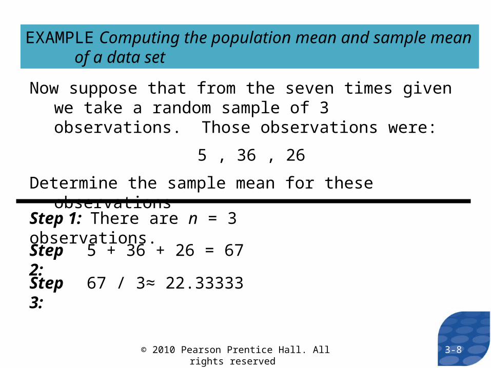
EXAMPLE Computing the population mean and sample mean of a data set
Now suppose that from the seven times given we take a random sample of 3 observations. Those observations were:
5 , 36 , 26
Determine the sample mean for these observations
Step 1: There are n = 3 observations.
Step 2:
3-8© 2010 Pearson Prentice Hall. All rights reserved
5 + 36 + 26 = 67
Step 3: 67 / 3≈ 22.33333

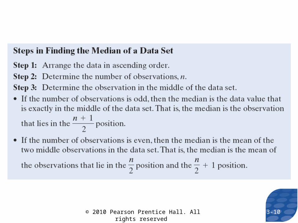
The median of a variable is the value that lies in the middle of the data when arranged in ascending order. We use M to represent the median.
3-9© 2010 Pearson Prentice Hall. All rights reserved
3-10© 2010 Pearson Prentice Hall. All rights reserved

EXAMPLE Computing a Median of a Data Set with an Odd Number of Observations
The following data represent the travel times (in minutes) to work for all seven employees of a start-up web development company.
23, 36, 23, 18, 5, 26, 43
Determine the median of this data.
Step 1: 5, 18, 23, 23, 26, 36, 43
Step 2: There are n = 7 observations.
1 7 14
2 2
n Step 3: M = 23
5, 18, 23, 23, 26, 36, 43
3-11© 2010 Pearson Prentice Hall. All rights reserved

EXAMPLE Computing a Median of a Data Set with an Even Number of Observations
Suppose the start-up company hires a new employee. The travel time of the new employee is 70 minutes. Determine the median of the “new” data set.
23, 36, 23, 18, 5, 26, 43, 70
Step 1: 5, 18, 23, 23, 26, 36, 43, 70
Step 2: There are n = 8 observations.
1 8 14.5
2 2
n Step 3:
5, 18, 23, 23, 26, 36, 43, 70
23 2624.5 minutes
2M
24.5M
3-12© 2010 Pearson Prentice Hall. All rights reserved

EXAMPLE Computing a Median of a Data Set with an Even Number of Observations
The following data represent the travel times (in minutes) to work for all seven employees of a start-up web development company.
23, 36, 23, 18, 5, 26, 43
Suppose a new employee is hired who has a 130 minute commute. How does this impact the value of the mean and median?
Mean before new hire: 24.9 minutesMedian before new hire: 23 minutes
Mean after new hire: 38 minutesMedian after new hire: 24.5 minutes
3-13© 2010 Pearson Prentice Hall. All rights reserved
A numerical summary of data is said to be resistant if extreme values (very large or small) relative to the data do not affect its value substantially.
3-14© 2010 Pearson Prentice Hall. All rights reserved
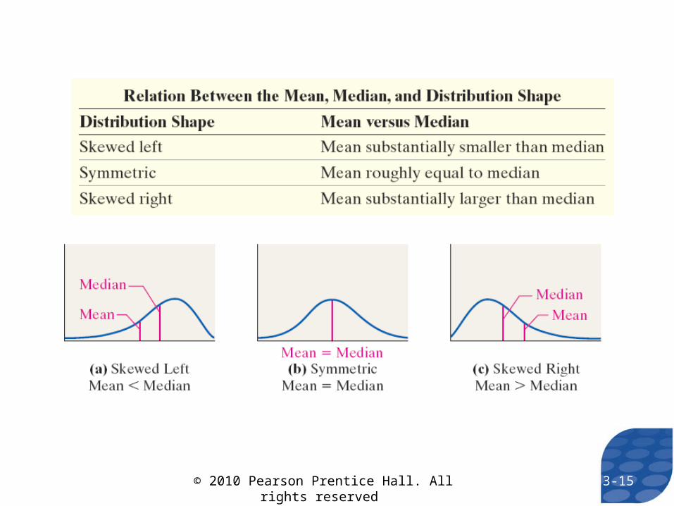
3-15© 2010 Pearson Prentice Hall. All rights reserved

EXAMPLE Describing the Shape of the Distribution
The following data represent the asking price of homes for sale in Lincoln, NE.
Source: http://www.homeseekers.com
79,995 128,950 149,900 189,900
99,899 130,950 151,350 203,950
105,200 131,800 154,900 217,500
111,000 132,300 159,900 260,000
120,000 134,950 163,300 284,900
121,700 135,500 165,000 299,900
125,950 138,500 174,850 309,900
126,900 147,500 180,000 349,900
3-16© 2010 Pearson Prentice Hall. All rights reserved

Find the mean and median. Use the mean and median to identify the shape of the distribution. Verify your result by drawing a histogram of the data.
3-17© 2010 Pearson Prentice Hall. All rights reserved

Find the mean and median. Use the mean and median to identify the shape of the distribution. Verify your result by drawing a histogram of the data.
The mean asking price is $168,320 and the median asking price is $148,700. Therefore, we would conjecture that the distribution is skewed right.
3-18© 2010 Pearson Prentice Hall. All rights reserved

350000300000250000200000150000100000
12
10
8
6
4
2
0
Asking Price
Frequency
Asking Price of Homes in Lincoln, NE
3-19© 2010 Pearson Prentice Hall. All rights reserved
The mode of a variable is the most frequent observation of the variable that occurs in the data set.
If there is no observation that occurs with the most frequency, we say the data has no mode.
3-20© 2010 Pearson Prentice Hall. All rights reserved

EXAMPLE Finding the Mode of a Data Set
The data on the next slide represent the Vice Presidents of the United States and their state of birth. Find the mode.
3-21© 2010 Pearson Prentice Hall. All rights reserved

3-22© 2010 Pearson Prentice Hall. All rights reserved

3-23© 2010 Pearson Prentice Hall. All rights reserved

The mode is New York.
3-24© 2010 Pearson Prentice Hall. All rights reserved
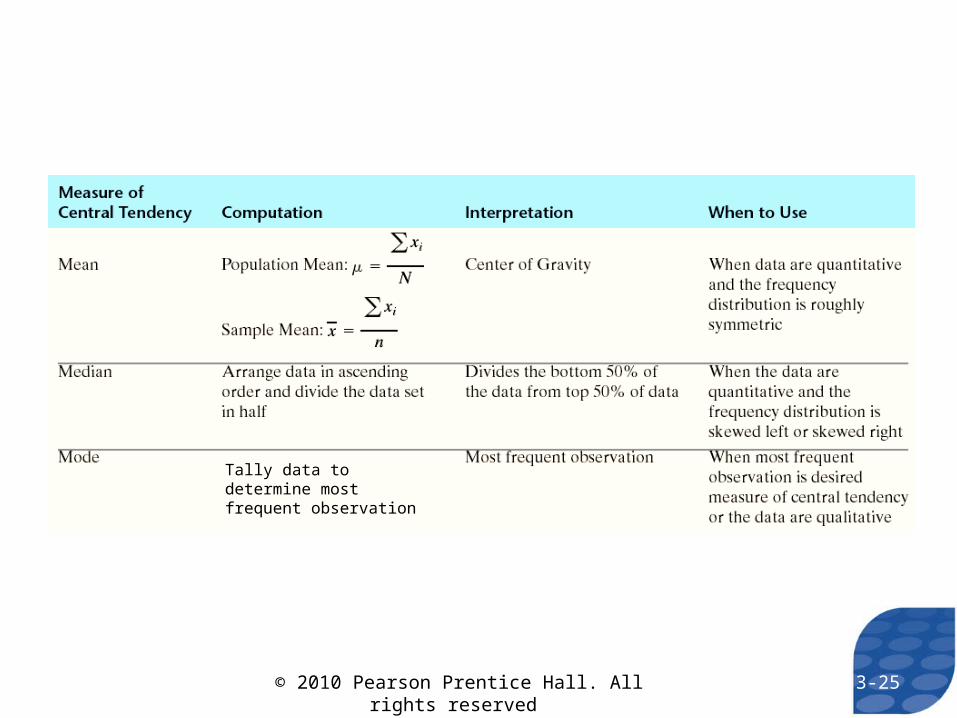
Tally data to determine most frequent observation
3-25© 2010 Pearson Prentice Hall. All rights reserved

The range, R, of a variable is the difference between the largest data value and the smallest data values. That is
Range = R = Largest Data Value – Smallest Data Value
3-26© 2010 Pearson Prentice Hall. All rights reserved
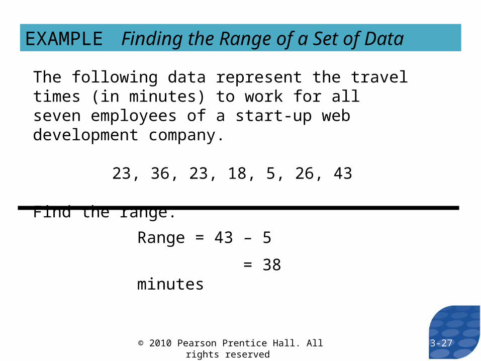
EXAMPLE Finding the Range of a Set of Data
The following data represent the travel times (in minutes) to work for all seven employees of a start-up web development company.
23, 36, 23, 18, 5, 26, 43
Find the range.
Range = 43 – 5
= 38 minutes
3-27© 2010 Pearson Prentice Hall. All rights reserved

The population variance of a variable is the sum of squared deviations about the population mean divided by the number of observations in the population, N.
That is it is the mean of the sum of the squared deviations about the population mean.
3-28© 2010 Pearson Prentice Hall. All rights reserved
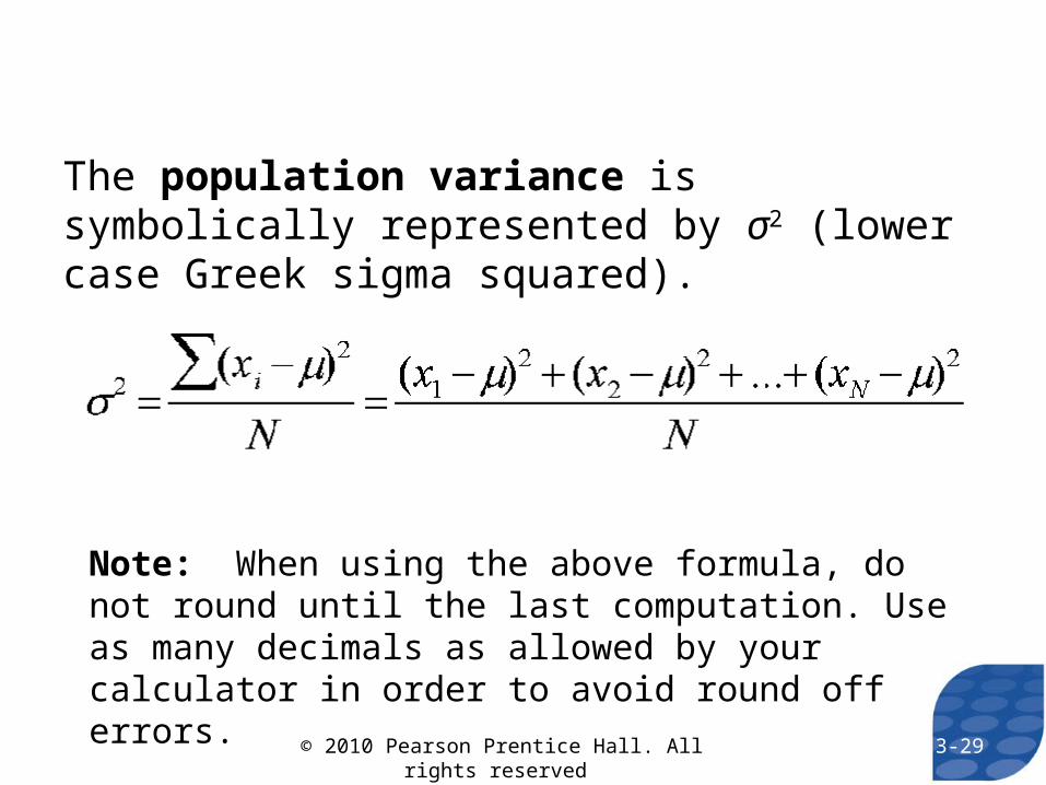
The population variance is symbolically represented by σ2 (lower case Greek sigma squared).
Note: When using the above formula, do not round until the last computation. Use as many decimals as allowed by your calculator in order to avoid round off errors.
3-29© 2010 Pearson Prentice Hall. All rights reserved

EXAMPLE Computing a Population Variance
The following data represent the travel times (in minutes) to work for all seven employees of a start-up web development company.
23, 36, 23, 18, 5, 26, 43
Compute the population variance of this data. Recall that
17424.85714
7
3-30© 2010 Pearson Prentice Hall. All rights reserved

xi μ xi – μ (xi – μ)2
23 24.85714 -1.85714 3.44898
36 24.85714 11.14286 124.1633
23 24.85714 -1.85714 3.44898
18 24.85714 -6.85714 47.02041
5 24.85714 -19.8571 394.3061
26 24.85714 1.142857 1.306122
43 24.85714 18.14286 329.1633
902.8571 2
ix 2
2 902.8571
7ix
N
129.0 minutes2
3-31© 2010 Pearson Prentice Hall. All rights reserved

The Computational Formula
3-32© 2010 Pearson Prentice Hall. All rights reserved

EXAMPLE Computing a Population Variance Using the Computational Formula
The following data represent the travel times (in minutes) to work for all seven employees of a start-up web development company.
23, 36, 23, 18, 5, 26, 43
Compute the population variance of this data using the computational formula.
3-33© 2010 Pearson Prentice Hall. All rights reserved

2 2 2 223 36 ... 43 5228ix
23, 36, 23, 18, 5, 26, 43
23 36 ... 43 174ix
22
2
2
1745228
77
i
i
xx
NN
129.0
3-34© 2010 Pearson Prentice Hall. All rights reserved

The sample variance is computed by determining the sum of squared deviations about the sample mean and then dividing this result by n – 1.
3-35© 2010 Pearson Prentice Hall. All rights reserved

Note: Whenever a statistic consistently overestimates or underestimates a parameter, it is called biased. To obtain an unbiased estimate of the population variance, we divide the sum of the squared deviations about the mean by n - 1.
3-36© 2010 Pearson Prentice Hall. All rights reserved
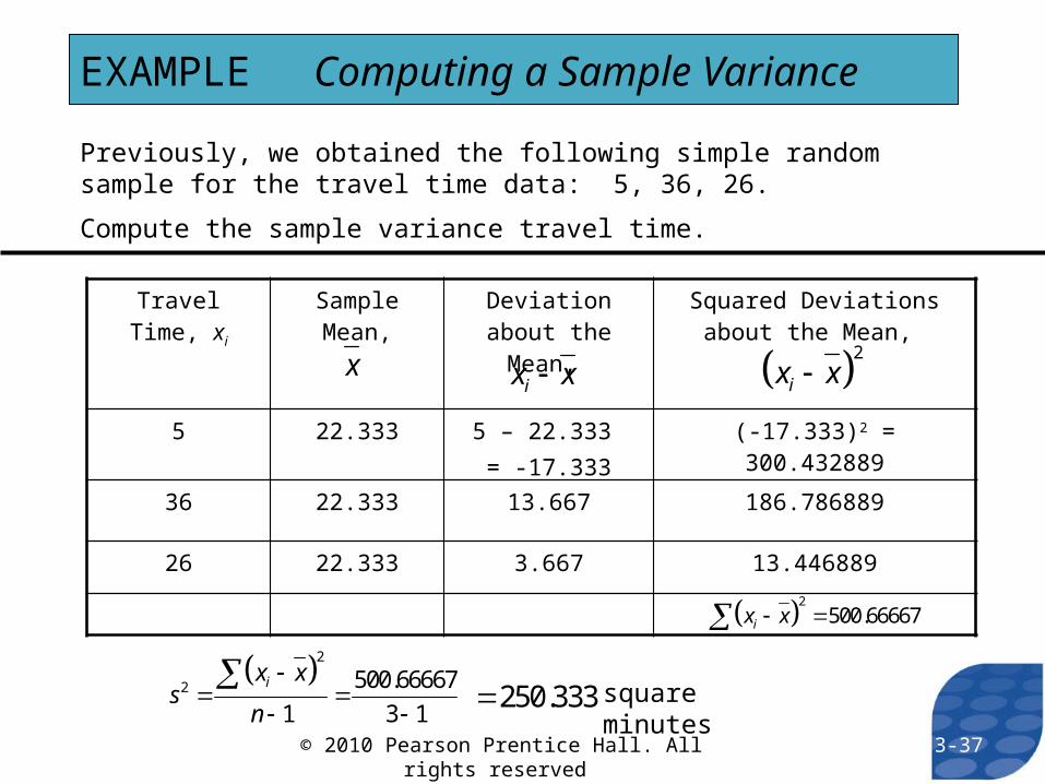
EXAMPLE Computing a Sample Variance
Previously, we obtained the following simple random sample for the travel time data: 5, 36, 26.
Compute the sample variance travel time.
Travel Time, xi Sample Mean, Deviation about the Mean,
Squared Deviations about the Mean,
5 22.333 5 – 22.333 = -17.333
(-17.333)2 = 300.432889
36 22.333 13.667 186.786889
26 22.333 3.667 13.446889
xix x 2
ix x
2500.66667ix x
2
2 500.66667
1 3 1
ix xs
n
250.333 square minutes
3-37© 2010 Pearson Prentice Hall. All rights reserved

The population standard deviation is denoted by
It is obtained by taking the square root of the population variance, so that
The sample standard deviation is denoted by
s
It is obtained by taking the square root of the sample variance, so that
2s s3-38© 2010 Pearson Prentice Hall. All rights reserved
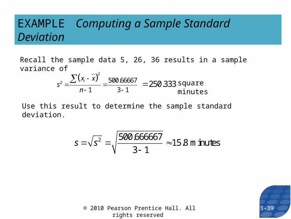
EXAMPLE Computing a Sample Standard Deviation
Recall the sample data 5, 26, 36 results in a sample variance of
2
2 500.66667
1 3 1
ix xs
n
250.333 square minutes
Use this result to determine the sample standard deviation.
2 500.66666715.8 minutes
3 1s s
3-39© 2010 Pearson Prentice Hall. All rights reserved

EXAMPLE Comparing Standard Deviations
Determine the standard deviation waiting time for Wendy’s and McDonald’s. Which is larger? Why?
3-40© 2010 Pearson Prentice Hall. All rights reserved
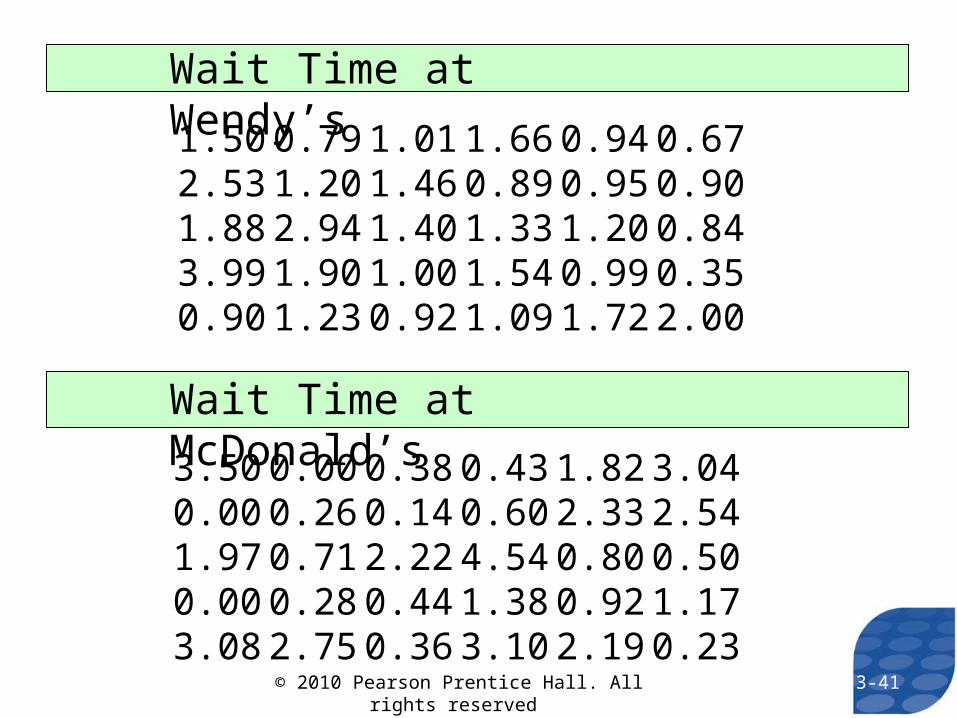
1.50 0.79 1.01 1.66 0.94 0.672.53 1.20 1.46 0.89 0.95 0.901.88 2.94 1.40 1.33 1.20 0.843.99 1.90 1.00 1.54 0.99 0.350.90 1.23 0.92 1.09 1.72 2.00
3.50 0.00 0.38 0.43 1.82 3.040.00 0.26 0.14 0.60 2.33 2.541.97 0.71 2.22 4.54 0.80 0.500.00 0.28 0.44 1.38 0.92 1.173.08 2.75 0.36 3.10 2.19 0.23
Wait Time at Wendy’s
Wait Time at McDonald’s
3-41© 2010 Pearson Prentice Hall. All rights reserved

EXAMPLE Comparing Standard Deviations
Determine the standard deviation waiting time for Wendy’s and McDonald’s. Which is larger? Why?
Sample standard deviation for Wendy’s:
0.738 minutes
Sample standard deviation for McDonald’s:
1.265 minutes
3-42© 2010 Pearson Prentice Hall. All rights reserved

Quartiles divide data sets into fourths, or four equal parts.
• The 1st quartile, denoted Q1, divides the bottom 25% the data from the top 75%. Therefore, the 1st quartile is equivalent to the 25th percentile.
• The 2nd quartile divides the bottom 50% of the data from the top 50% of the data, so that the 2nd quartile is equivalent to the 50th percentile, which is equivalent to the median.
• The 3rd quartile divides the bottom 75% of the data from the top 25% of the data, so that the 3rd quartile is equivalent to the 75th percentile.
3-43© 2010 Pearson Prentice Hall. All rights reserved

3-44© 2010 Pearson Prentice Hall. All rights reserved

A group of Brigham Young University—Idaho students (Matthew Herring, Nathan Spencer, Mark Walker, and Mark Steiner) collected data on the speed of vehicles traveling through a construction zone on a state highway, where the posted speed was 25 mph. The recorded speed of 14 randomly selected vehicles is given below:
20, 24, 27, 28, 29, 30, 32, 33, 34, 36, 38, 39, 40, 40
Find and interpret the quartiles for speed in the construction zone.
EXAMPLE Finding and Interpreting Quartiles
Step 1: The data is already in ascending order.
Step 2: There are n = 14 observations, so the median, or second quartile, Q2, is the mean of the 7th and 8th observations. Therefore, M = 32.5.
Step 3: The median of the bottom half of the data is the first quartile, Q1.
20, 24, 27, 28, 29, 30, 32
The median of these seven observations is 28. Therefore, Q1 = 28. The median of the top half of the data is the third quartile, Q3. Therefore, Q3 = 38.
3-45© 2010 Pearson Prentice Hall. All rights reserved

Interpretation:
• 25% of the speeds are less than or equal to the first quartile, 28 miles per hour, and 75% of the speeds are greater than 28 miles per hour.
• 50% of the speeds are less than or equal to the second quartile, 32.5 miles per hour, and 50% of the speeds are greater than 32.5 miles per hour.
• 75% of the speeds are less than or equal to the third quartile, 38 miles per hour, and 25% of the speeds are greater than 38 miles per hour.
3-46© 2010 Pearson Prentice Hall. All rights reserved
3-47© 2010 Pearson Prentice Hall. All rights reserved

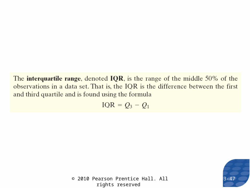
EXAMPLE Determining and Interpreting the Interquartile Range
Determine and interpret the interquartile range of the speed data.
Q1 = 28 Q3 = 38
3 1IQR
38 28
10
Q Q
The range of the middle 50% of the speed of cars traveling through the construction zone is 10 miles per hour.
3-48© 2010 Pearson Prentice Hall. All rights reserved
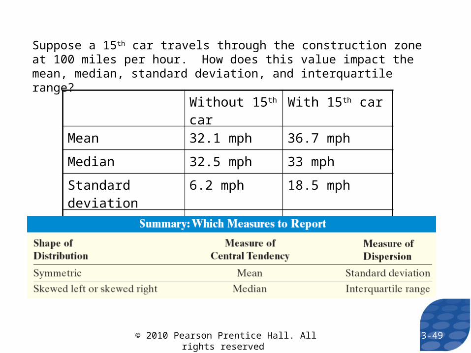
Suppose a 15th car travels through the construction zone at 100 miles per hour. How does this value impact the mean, median, standard deviation, and interquartile range?
Without 15th car With 15th car
Mean 32.1 mph 36.7 mph
Median 32.5 mph 33 mph
Standard deviation 6.2 mph 18.5 mph
IQR 10 mph 11 mph
3-49© 2010 Pearson Prentice Hall. All rights reserved

3-50© 2010 Pearson Prentice Hall. All rights reserved

EXAMPLE Determining and Interpreting the Interquartile Range
Check the speed data for outliers.
Step 1: The first and third quartiles are Q1 = 28 mph and Q3 = 38 mph.
Step 2: The interquartile range is 10 mph.
Step 3: The fences are
Lower Fence = Q1 – 1.5(IQR) Upper Fence = Q3 + 1.5(IQR)
= 28 – 1.5(10) = 38 + 1.5(10)
= 13 mph = 53 mph
Step 4: There are no values less than 13 mph or greater than 53 mph. Therefore, there are no outliers.
3-51© 2010 Pearson Prentice Hall. All rights reserved

3-52© 2010 Pearson Prentice Hall. All rights reserved

EXAMPLE Obtaining the Five-Number Summary
Every six months, the United States Federal Reserve Board conducts a survey of credit card plans in the U.S. The following data are the interest rates charged by 10 credit card issuers randomly selected for the July 2005 survey. Determine the five-number summary of the data.
Institution Rate
Pulaski Bank and Trust Company 6.5%
Rainier Pacific Savings Bank 12.0%
Wells Fargo Bank NA 14.4%
Firstbank of Colorado 14.4%
Lafayette Ambassador Bank 14.3%
Infibank 13.0%
United Bank, Inc. 13.3%
First National Bank of The Mid-Cities 13.9%
Bank of Louisiana 9.9%
Bar Harbor Bank and Trust Company 14.5%
Source: http://www.federalreserve.gov/pubs/SHOP/survey.htm
First, we write the data is ascending order:
6.5%, 9.9%, 12.0%, 13.0%, 13.3%, 13.9%, 14.3%, 14.4%, 14.4%, 14.5%
The smallest number is 6.5%. The largest number is 14.5%. The first quartile is 12.0%. The second quartile is 13.6%. The third quartile is 14.4%.
Five-number Summary:
6.5% 12.0% 13.6% 14.4% 14.5%
3-53© 2010 Pearson Prentice Hall. All rights reserved

3-54© 2010 Pearson Prentice Hall. All rights reserved

EXAMPLE Constructing a Boxplot
Every six months, the United States Federal Reserve Board conducts a survey of credit card plans in the U.S. The following data are the interest rates charged by 10 credit card issuers randomly selected for the July 2005 survey. Draw a boxplot of the data.
Institution Rate
Pulaski Bank and Trust Company 6.5%
Rainier Pacific Savings Bank 12.0%
Wells Fargo Bank NA 14.4%
Firstbank of Colorado 14.4%
Lafayette Ambassador Bank 14.3%
Infibank 13.0%
United Bank, Inc. 13.3%
First National Bank of The Mid-Cities 13.9%
Bank of Louisiana 9.9%
Bar Harbor Bank and Trust Company 14.5%
Source: http://www.federalreserve.gov/pubs/SHOP/survey.htm
3-55© 2010 Pearson Prentice Hall. All rights reserved

Step 1: The interquartile range (IQR) is 14.4% - 12% = 2.4%. The lower and upper fences are:
Lower Fence = Q1 – 1.5(IQR) Upper Fence = Q3 + 1.5(IQR)
= 12 – 1.5(2.4) = 14.4 + 1.5(2.4)
= 8.4% = 18.0%
Step 2:
[ ]*
3-56© 2010 Pearson Prentice Hall. All rights reserved
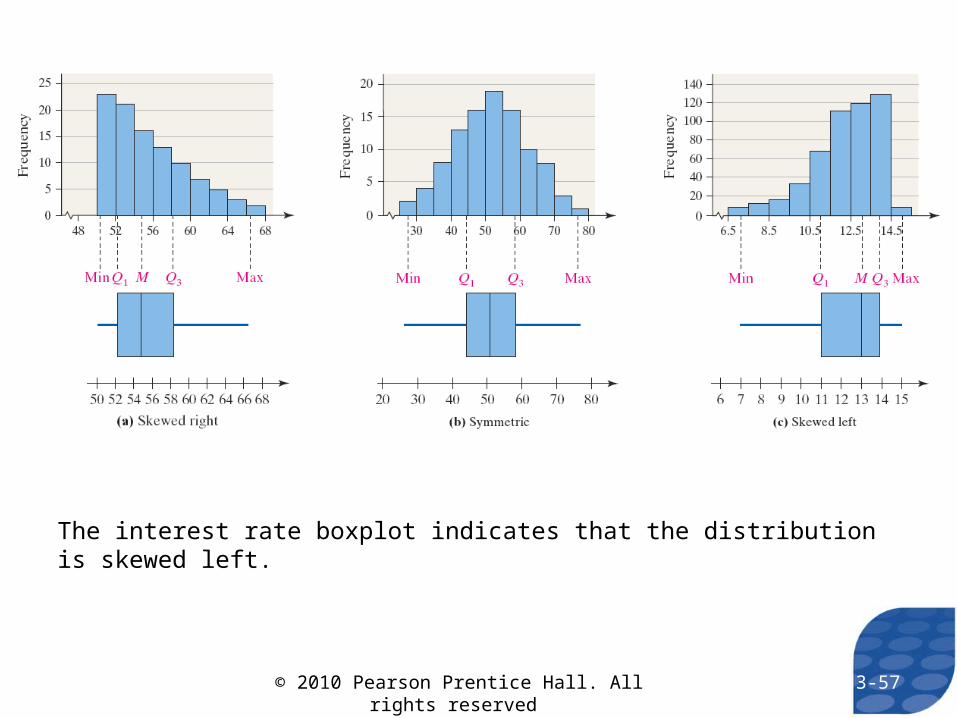
The interest rate boxplot indicates that the distribution is skewed left.
3-57© 2010 Pearson Prentice Hall. All rights reserved
3-58© 2010 Pearson Prentice Hall. All rights reserved
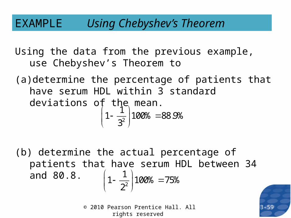
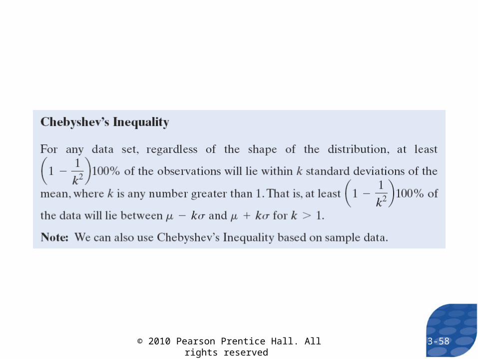
EXAMPLE Using Chebyshev’s Theorem
Using the data from the previous example, use Chebyshev’s Theorem to
(a) determine the percentage of patients that have serum HDL within 3 standard deviations of the mean.
(b) determine the actual percentage of patients that have serum HDL between 34 and 80.8.
2
11 100% 88.9%
3
2
11 100% 75%
2
3-59© 2010 Pearson Prentice Hall. All rights reserved

3-60© 2010 Pearson Prentice Hall. All rights reserved

3-61© 2010 Pearson Prentice Hall. All rights reserved

EXAMPLE Using the Empirical RuleThe following data represent the serum HDL cholesterol of the 54 female patients of a family doctor.
41 48 43 38 35 37 44 44 4462 75 77 58 82 39 85 55 5467 69 69 70 65 72 74 74 7460 60 60 61 62 63 64 64 6454 54 55 56 56 56 57 58 5945 47 47 48 48 50 52 52 53
3-62© 2010 Pearson Prentice Hall. All rights reserved

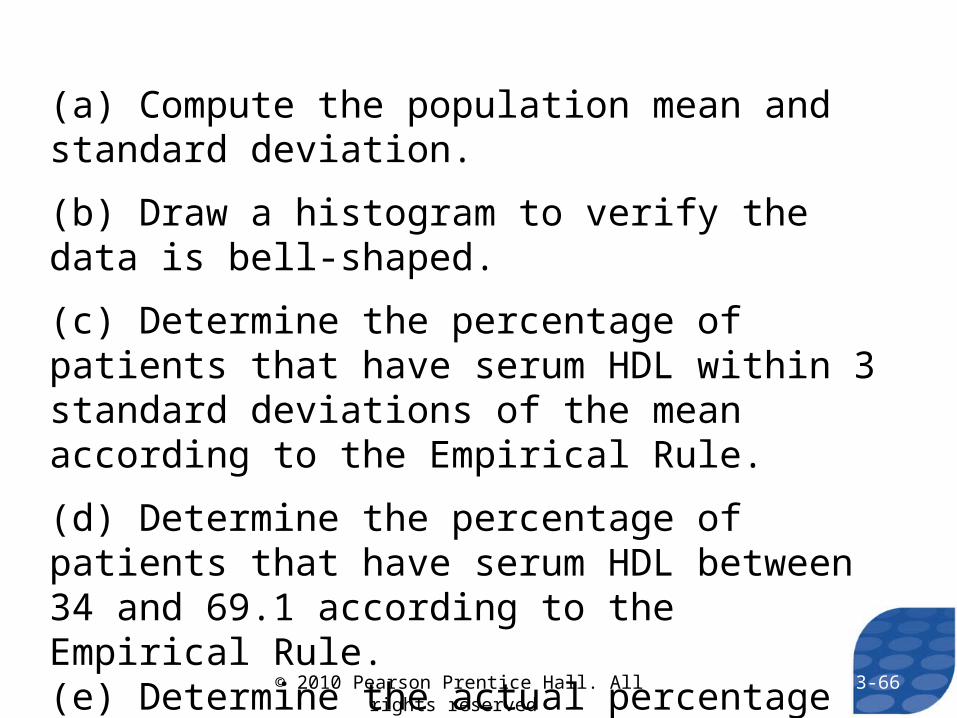
(a) Compute the population mean and standard deviation.
(b) Draw a histogram to verify the data is bell-shaped.
(c) Determine the percentage of patients that have serum HDL within 3 standard deviations of the mean according to the Empirical Rule.
(d) Determine the percentage of patients that have serum HDL between 34 and 69.1 according to the Empirical Rule. (e) Determine the actual percentage of patients that have serum HDL between 34 and 69.1.
3-63© 2010 Pearson Prentice Hall. All rights reserved

3-64© 2010 Pearson Prentice Hall. All rights reserved

EXAMPLE Using the Empirical RuleThe following data represent the serum HDL cholesterol of the 54 female patients of a family doctor.
41 48 43 38 35 37 44 44 4462 75 77 58 82 39 85 55 5467 69 69 70 65 72 74 74 7460 60 60 61 62 63 64 64 6454 54 55 56 56 56 57 58 5945 47 47 48 48 50 52 52 53
3-65© 2010 Pearson Prentice Hall. All rights reserved
(a) Compute the population mean and standard deviation.
(b) Draw a histogram to verify the data is bell-shaped.
(c) Determine the percentage of patients that have serum HDL within 3 standard deviations of the mean according to the Empirical Rule.
(d) Determine the percentage of patients that have serum HDL between 34 and 69.1 according to the Empirical Rule. (e) Determine the actual percentage of patients that have serum HDL between 34 and 69.1.
3-66© 2010 Pearson Prentice Hall. All rights reserved

(a) Using the formulas for mean and standard deviation
(b)
7.11 and 4.57
3-67© 2010 Pearson Prentice Hall. All rights reserved
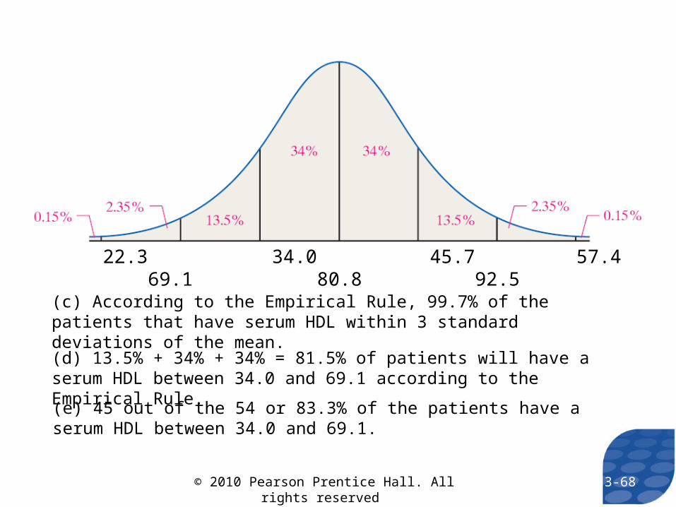
22.3 34.0 45.7 57.4 69.1 80.8 92.5
(e) 45 out of the 54 or 83.3% of the patients have a serum HDL between 34.0 and 69.1.
(c) According to the Empirical Rule, 99.7% of the patients that have serum HDL within 3 standard deviations of the mean.
(d) 13.5% + 34% + 34% = 81.5% of patients will have a serum HDL between 34.0 and 69.1 according to the Empirical Rule.
3-68© 2010 Pearson Prentice Hall. All rights reserved
3-69© 2010 Pearson Prentice Hall. All rights reserved

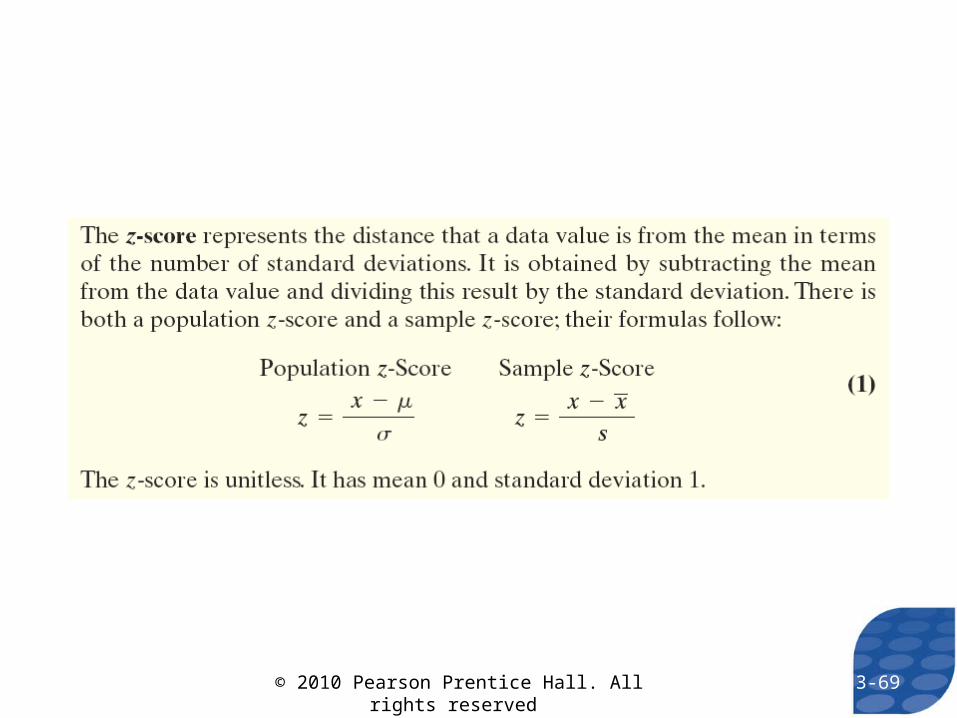
EXAMPLE Using Z-Scores
The mean height of males 20 years or older is 69.1 inches with a standard deviation of 2.8 inches. The mean height of females 20 years or older is 63.7 inches with a standard deviation of 2.7 inches. Data based on information obtained from National Health and Examination Survey. Who is relatively taller?
Kevin Garnett whose height is 83 inches
or
Candace Parker whose height is 76 inches
3-70© 2010 Pearson Prentice Hall. All rights reserved

83 69.1
2.84.96
kgz
76 63.7
2.74.56
cpz
Kevin Garnett’s height is 4.96 standard deviations above the mean. Candace Parker’s height is 4.56 standard deviations above the mean. Kevin Garnett is relatively taller.
3-71© 2010 Pearson Prentice Hall. All rights reserved

The kth percentile, denoted, Pk, of a set of data is a value such that k percent of the observations are less than or equal to the value.
3-72© 2010 Pearson Prentice Hall. All rights reserved