yukon ecological monitoring protocolskrebs/downloads/field_manual_2016-short.pdf · the kluane...

Yukon Ecological Monitoring PROTOCOLS

(2016 edition)

Ecological Monitoring Protocols Page 1

Table of Contents Table of Contents 1

Background - The Community Ecological Monitoring Project 2

Monitoring Schedule 4

Typical Snowshoe Hare Trapping Grid Layout 5

Typical 100 Station Transect Layout 6

Compass Bearings and Distances 7

General Field and Data Entry Techniques 8

Spruce Cone Production Sampling 9

Mushroom Counts Protocol 13

Ground Berry Production Protocol 18

Soapberry Production Protocol 24

Snowshoe Hare Pellet Counts 28

Mouse Trapping Protocol 31

Ecological Monitoring Protocols

Background - The Community Ecological Monitoring Project In 1973 ecologists from the University of British Columbia began working on the small mammals of the Kluane area. In 1986 a group of nine ecologists from the University of British Columbia, the University of Alberta, and the University of Toronto collaborated to expand the research with support from the Natural Sciences and Engineering Research Council of Canada. This new study was called the "Kluane Boreal Forest Ecosystem Project" and continued until 1996. The focus of the Kluane Boreal Forest Ecosystem Project was to understand the community structure of the vertebrates that live in the boreal forest around Kluane Lake in the southwestern Yukon. The key focus of all this research for the past 37 years has been the snowshoe hare, which undergoes 9-10 year cycles throughout the boreal forest of Canada. The snowshoe hare is a keystone herbivore in this system, and has potential impacts on other species either through competition for food through its browsing on plants or through predators that eat hares as well as other prey species (Figure 1). In the early 1990s the spruce bark beetle began to outbreak in the Kluane area, killing mature spruce trees in a patchy manner throughout the Shakwak Trench. This major disturbance to the ecosystem is only slowly working its effects on other species in the food chain, and is one of the centers of attention for the project that developed starting in 1996 – the "Kluane Ecological Monitoring Project".

The Kluane Ecological Monitoring Project (KEMP) attempts to census the major plants and animals in the boreal forests of Kluane in order to provide a long term baseline of ecosystem change. Our working hypothesis is that the boreal forest community is never in equilibrium because of disturbances caused by fire and bark beetle outbreaks, and we need long-term data to follow these changes. Major climatic change is predicted to occur in the coming decades, and we need information on how the biological systems of the Canadian north are responding to climatic fluctuations. Because of the extensive background of information from the Kluane Project of 1986-96, we can build a monitoring project of international importance in this region.

The KEMP project has evolved since 1999 into a partnership between the University of British Columbia, University of Alberta, University of Toronto, Yukon College, Parks Canada, Yukon Department of Environment and the Canadian Wildlife Service. From 2004 to 2008 we received funding from


the Northern Ecosystem Initiative of Environment Canada and we are grateful for their support. The EJLB Foundation of Toronto supported our monitoring efforts from 2004 to 2009. The focus has now broadened geographically to several areas of the southern Yukon and the project is now called the “Community Ecological Monitoring Project” (CEMP) with the major support now from the Yukon Department of the Environment. In 2008 we reduced the number of protocols used to monitor the system.

Protocols - We include here a brief description of the protocols for the monitoring procedures of this project. Most of these procedures are based on similar methods evolved over the earlier studies at Kluane. We would appreciate feedback on how to improve these methods, what more might be included and how the descriptions could be improved. All data are stored in MS ACCESS databases. For each type of data collected, the database includes data sheets which can be printed and taken into the field, data entry forms, as well as appropriate summary statistics and reports.

Figure 1. Food web for Kluane region. Links are drawn between species if the species consumed constitutes at least 5% of the consumer’s diet. The major species are shown in yellow boxes.

Charles J. Krebs [email protected] March 2013

SNOWSHOEHARE

BOGBIRCH

GREYWILLOW

COYOTE

GOSHAWKRED FOX

RED-TAILEDHAWK WOLF

WHITESPRUCE

GREAT-HORNED OWL

LYNX

FORBS SOAPBERRY

NORTHERNHARRIER

WOLVERINE

SMALLRODENTS

REDSQUIRREL

GROUNDSQUIRREL

WILLOWPTARMIGAN

SPRUCEGROUSE

PASSERINEBIRDS

BALSAMPOPLAR ASPENGRASSES

HAWK OWLGOLDENEAGLE

KESTREL

INSECTS

MOOSE

FUNGI

GRIZZZLY


Monitoring Schedule January snow track transects for predators

February snow track transects write annual report

March snow track transects hare trapping owl census

April + May mouse trapping

June squirrel trapping

July ground berry production soapberry production spruce seedling growth and survival spruce cone production hare pellet transects

August mouse trapping squirrel trapping mushroom counts ground berry production collect ripe soapberries

September

October hare trapping

November snow track transects

December snow track transects


Typical Snowshoe Hare Trapping Grid Layout

The 86 rectangles on this diagram show the placement of the hare live-traps. The “traps” are coloured red if they are on a row flagged with red flagging tape or blue if they are on a row flagged with blue flagging tape (“odd” rows such as A,C,E… are flagged in red, “even” rows such as B,D,F… are flagged in blue). Grid spacing is 30m.


Typical 100 Station Transect Layout

The red dots in this diagram represent the 50 stations (marked in the field with wooden stakes). Stations are 15m apart and the two transects are 100m apart.

Some areas have four transects (each with 25 stations) instead of two transects.


Compass Bearings and Distances We often use a compass bearing and distance from a marker to help locate things we are measuring such as ground berry plots or cone trees. These bearings and distances are guides only and do not need to be perfectly precise. However, if the bearing is completely inaccurate then we potentially waste a lot of time looking for something in the wrong place.

How to take a compass bearing from a marker point to a tree (or plot):

Note that a full circle is 360 degrees (90=East, 180=South, 270=West, 360=North).

• Stand at the marker (typically a wood stake) and face the tree • Hold the compass level and point it toward the tree. • Turn the degree dial until the orienting lines are lined up with the

magnetic needle as shown above • Read the bearing off the degree dial. In the diagram above, the

tree is NW from the marker, or about 315 degrees

Measuring distances to plots or trees: It is useful to know roughly how far in meters the tree or plot is from the Marker. Take a few minutes at the beginning of the field season to measure how long your stride is (how many steps you take per meter). Walk from the Marker to the plot or tree and estimate the distance (in meters) based on your stride length. This is a guide for locating things in the future and does not have to be precise or perfectly accurate.


General Field and Data Entry Techniques • Data sheets contain the key records of all of our efforts. It is important

that they be filled in completely and clearly, your full name is on them, the date (including the year), and any special notations are explained. Make sure data sheets are reviewed at the end of each day so that any problems can be fixed while the details are still fresh in your memory.

• Any monitoring program must be concerned about the “Big Foot” effect - that our walking through the area may cause changes in the habitat. A major worry is establishing a trail down the sampling lines. Try to minimize trampling near the sampling stations and walk off the line when possible.

• You may be able to make interesting natural history observations in the course of doing this monitoring or in your other activities. Please put comments in the “General Comments” section of each data entry form in the Access database so that, for example, we will have a record of insect defoliation or high moose or grouse numbers at specific sites.

• Most data sheets have comments carried forward from the previous year, which may be relevant to the current year as well. Make a note on the data sheet if the comment is still relevant and therefore should be entered again for the current year. Comments are not automatically carried forward when entering the data into the computer.

• For some protocols we record a bearing from the grid or line marker to help locate the plot. These bearings are a guide only so they do not need to be precise.

• Use “-99” for missing data in the database. Never use “0” because that could be confused with actual data and confound the data analysis.


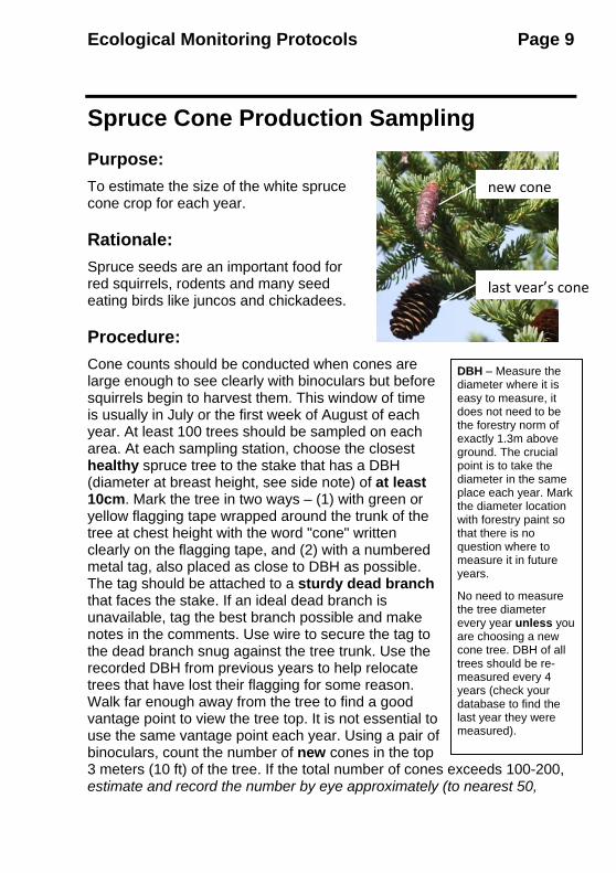
Spruce Cone Production Sampling Purpose: To estimate the size of the white spruce cone crop for each year.

Rationale: Spruce seeds are an important food for red squirrels, rodents and many seed eating birds like juncos and chickadees.

Procedure: Cone counts should be conducted when cones are large enough to see clearly with binoculars but before squirrels begin to harvest them. This window of time is usually in July or the first week of August of each year. At least 100 trees should be sampled on each area. At each sampling station, choose the closest healthy spruce tree to the stake that has a DBH (diameter at breast height, see side note) of at least 10cm. Mark the tree in two ways – (1) with green or yellow flagging tape wrapped around the trunk of the tree at chest height with the word "cone" written clearly on the flagging tape, and (2) with a numbered metal tag, also placed as close to DBH as possible. The tag should be attached to a sturdy dead branch that faces the stake. If an ideal dead branch is unavailable, tag the best branch possible and make notes in the comments. Use wire to secure the tag to the dead branch snug against the tree trunk. Use the recorded DBH from previous years to help relocate trees that have lost their flagging for some reason. Walk far enough away from the tree to find a good vantage point to view the tree top. It is not essential to use the same vantage point each year. Using a pair of binoculars, count the number of new cones in the top 3 meters (10 ft) of the tree. If the total number of cones exceeds 100-200, estimate and record the number by eye approximately (to nearest 50,

DBH – Measure the diameter where it is easy to measure, it does not need to be the forestry norm of exactly 1.3m above ground. The crucial point is to take the diameter in the same place each year. Mark the diameter location with forestry paint so that there is no question where to measure it in future years.

No need to measure the tree diameter every year unless you are choosing a new cone tree. DBH of all trees should be re-measured every 4 years (check your database to find the last year they were measured).

new cone

last year’s cone


spend no more than 10 seconds on this estimate) and take a photograph of the top of the tree so cones can be counted later with more ease and accuracy. Write the estimate and the photo number on the data sheet as well as a note that a photo was taken.

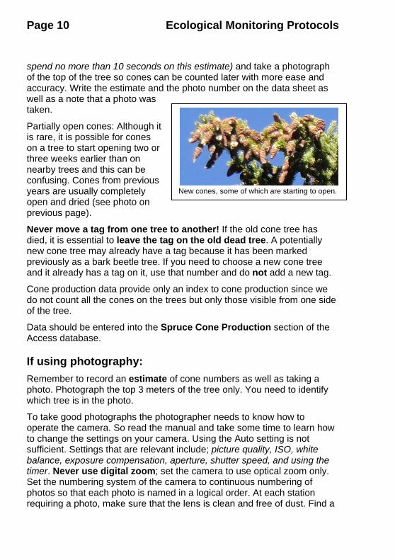
Partially open cones: Although it is rare, it is possible for cones on a tree to start opening two or three weeks earlier than on nearby trees and this can be confusing. Cones from previous years are usually completely open and dried (see photo on previous page).

Never move a tag from one tree to another! If the old cone tree has died, it is essential to leave the tag on the old dead tree. A potentially new cone tree may already have a tag because it has been marked previously as a bark beetle tree. If you need to choose a new cone tree and it already has a tag on it, use that number and do not add a new tag.

Cone production data provide only an index to cone production since we do not count all the cones on the trees but only those visible from one side of the tree.

Data should be entered into the Spruce Cone Production section of the Access database.

If using photography: Remember to record an estimate of cone numbers as well as taking a photo. Photograph the top 3 meters of the tree only. You need to identify which tree is in the photo.

To take good photographs the photographer needs to know how to operate the camera. So read the manual and take some time to learn how to change the settings on your camera. Using the Auto setting is not sufficient. Settings that are relevant include; picture quality, ISO, white balance, exposure compensation, aperture, shutter speed, and using the timer. Never use digital zoom; set the camera to use optical zoom only. Set the numbering system of the camera to continuous numbering of photos so that each photo is named in a logical order. At each station requiring a photo, make sure that the lens is clean and free of dust. Find a

New cones, some of which are starting to open.


good spot with the majority of the light coming from behind you and where you have a clear, unobstructed view of the top three meters of the tree. Use a tripod and the timer function on the camera to avoid camera shake is if there is not enough light for a fast shutter speed. If you are worried about exposure of the photos, take several photos of the tree with bracketed exposure settings. If the tree is moving due to wind, try using the sports setting to increase the shutter speed. Check to be sure that the image is clear by zooming in to full extent on. Do this for every single photo taken!

Use a minimum 3 megapixel camera, preferably 5 megapixels or more, with a minimum 3x optical zoom, preferably 10x. Record the name of the photos (eg Img001, Img002) on the data sheet.

Cones can be counted on the computer by opening the photo in a bitmap editor such as MS Paint and placing a dot on each cone as it is counted. Use an automatic mouse click counter such as OdoPlus (http://www.fridgesoft.de/odoplus.php - this program has also been stored on our Zeus file backup system).

Make sure when using a clicker counter to RESET to zero at the start of counting cones on a tree. If using OdoPlus, it works best to use the right mouse button for counting and reserve the left mouse button for scrolling (“color 2” on the Windows 7 version of the Paint program uses the right mouse button).

Summary Statistics: The bootstrapped mean number of cones (and 95% confidence intervals) for each area and year is computed under the “Summary Statistics” option of the CEMP_data Access database.

Equipment: Data Sheets Binoculars Flagging Tape: Yellow or Green Marker Pen Clicker counters DBH tape for measuring tree diameter Camera with telephoto lens & tripod Aluminum tags Hammer

http://www.fridgesoft.de/odoplus.php


Time Estimates: Field: 1 person day per area Lab: up to 2 person days per area (if photos taken) Data Entry and analysis: ½ person day per area


Mushroom Counts Protocol Purpose: To estimate the standing crop of mushrooms (grams per 10 sq meters) at the peak of the mushroom season.

Rationale: Mushrooms are an important alternate food for red squirrels and small rodents, and their abundance varies greatly from year to year.

Procedure: Mushrooms should be counted at the peak of the mushroom season, which is normally August 1-15 at Kluane. Some preliminary surveys may be needed to pinpoint the maximum time of mushroom emergence. There is a timing trade off - count too early and you will miss mushrooms that haven't yet emerged, count too late and some mushrooms will already be harvested by squirrels.

The quadrat is a circle of 3 meters radius centered on the grid (or transect) marker stake. Use a 3m piece of non-stretchable string or tape pinned to the stake to locate the outer edge of the quadrat. At least 100 quadrats should be counted on each area. Within each circle count all the mushrooms that are visible of ALL SPECIES* and measure their cap diameters in cm (to one decimal point) in order to classify the mushrooms into the following three size classes: SMALL (<4 cm), MEDIUM (>=4 and <8 cm) and LARGE (>=8 cm). If the mushroom is oblong, measure two

diameters and average them. Record in cm to one decimal place.

SMALL and MEDIUM mushrooms: Record the number of small and medium sized mushrooms counted in the quadrat at each station. In order to convert the numbers to biomass, you need to precisely measure the diameters of a subset of 20-40 small mushrooms and 20-40 medium

* See end of this section (page 18) for exceptions!


mushrooms. Repeat this for each area and enter the diameters into the Access database. If there are fewer than 20 small or medium mushrooms on a particular area, then take diameters of all mushrooms counted at that site. There is no need to measure mushrooms outside of the quadrats to get more diameters. If there are huge numbers of mushrooms, do not take all the diameters from the first station, instead spread the measurements spatially by taking 2-3 diameters at each station until you have enough.

LARGE mushrooms (>=8cm diameter): Because large sized mushrooms can make up most of the biomass produced, you need to record the

diameter of every large mushroom. This will ensure the final biomass estimates are as accurate as possible.

NOTE: If you find a stalk of a mushroom that has obviously been already harvested by squirrels, count the mushroom as a medium (it may have been large but this is conservative). We do not count mushrooms growing on tree trunks or tree limbs because they are woody bracket fungi, and they are not eaten by any animals that we know of.

Data Entry: All count data and sample diameter measurements (small and mediums sized mushrooms) should be entered into the Access database. When you enter the number of large sized mushrooms counted, a box will pop up asking for each individual diameter (cm).

Summary Statistics (Biomass Estimates): The wet weight of a large mushroom is calculated using the following formulas:

Mushroom Cap Area = 3.1415927 * ([Cap Diameter] / 2) * ([Cap Diameter] / 2)

Wet Weight = 1.095023 * (Exp(-1.06392 + (1.200234 * Log(Cap Area))))

(correlation coefficient R = 0.94) Diameters are in cm and weights are in grams.

The wet weight regression is based on Kluane data compiled by Patrick Carrier for his MSc in 1995 and with additional data gathered in 1997 and 2000. Once all count and diameter data are entered, the bootstrapped mean biomass per 10 m2 (standing crop) and 95% confidence interval for

Old or New? If a mushroom is dry, shriveled and hard then assume it is from last year. If it is fleshy, even if rotten, assume it is from this year.


each area and year is computed under the “Summary Statistics” option of the CEMP_data Access database.

Equipment: Data sheets & pencils Non stretchable string - exactly 3m in length Thumb tack for pinning string to stake Ruler Clicker (tally counter)

Time Estimates: Field: 2-4 person days per area Data Entry: ½ person day per area

Mushrooms that we do NOT count: We do not count any mushrooms <2 mm in diameter. Also exclude the following species because we do not have diameter to biomass regressions for these species and we have no indication that these species are important food sources for small mammals.

Coral mushrooms Puffballs

Do not count these mushroom species but make notes about them in the comments field (including an estimate of the numbers or size).

Gold fingers


Ground Berry Production Protocol Purpose: To obtain an index of ground berry production each year.

Rationale: Ground berries are an important food for small mammals and production varies greatly from year to year.

Procedure: We count the number of berries produced in permanent quadrats in the boreal forest each year to give an index of berry production. We do not attempt to measure the total biomass production of ground berries per hectare.

Timing: The berries should be counted each summer when the plants have finished flowering. We've tested counting flowers but they are not a reliable predictor of final berry production. It is also preferable that the berries are still green when counted in order to minimize the amount of harvesting by mice which occurs once the berries begin to ripen in August. The optimal timing of counts may vary from year to year and some monitoring in late June to mid July should give a good estimate of when counts should be conducted. Arctostaphylos uva-ursi and Empetrum generally will ripen earlier than other species while Cornus and Vaccinium generally ripen late in the summer. For each region the optimal timing for berry counts may be different by up to two or three weeks and it is important to make detailed comments about phenology at each site for each year.

Ground berries are monitored in permanent 0.4 x 0.4 meter square quadrats. Look for a good berry patch with at least 50% cover of one of the target species (see side note on page 20) within 5-7 meters of the grid or transect marker and place two quadrats side by side. Mark a nearby bush or tree with unique (eg. polkadot) flagging tape to indicate where the quadrats are located. Mark the quadrats with 4 spikes - one BLUE flagged spike at each outer corner of the quadrat closest to the transect marker (quadrat # 1),

Berries on the edge are counted if at least ½ of the berry is inside the quadrat.

Flowers: Do not count flowers because they do not reliably turn into berries.

Bits & Pieces: When berries are harvested by mice sometimes small bits are left on the ground. Count these piles conservatively as 1 berry.


and one RED flagged spike at each outer corner of the adjoining quadrat (quadrat # 2). You will now have a 0.4 by 0.8 meter rectangle marked containing two quadrats. Estimate the distance in meters from the transect marker to the nearest quadrat (#1) and record the approximate compass bearing from the transect marker to the quadrats so we can locate the quadrats easily the following year. One hundred quadrats (50 sites, each with 2 quadrats) should be measured in each area. Note that not every transect marker will have a set of ground berry quadrats – only good sites are used.

In each quadrat, estimate the percent cover of each berry producing species and count the berries. All berries should be counted, including shriveled or tiny or dropped and over-wintered ones. Do this for each berry species - Arctostaphylos uva-ursi (kinnikinick), Arctostaphylos rubra (red bearberry), Empetrum nigrum (mossberry, crowberry), Geocaulon lividum (toadflax), Vaccinium vitis-idaea (cranberry), Cornus canadensis (bunchberry). In the “Other” category include only blueberry, strawberry and rose. If two “Other” species occur in one plot, record the second species in the Comments field.

When to move a quadrat: We compare berry production in the same quadrats each year so, if at all possible, they should never be moved. If a tree falls on top of the quadrat so that it's impossible to count the berries or if it is destroyed for some reason, then it will have to be moved. Be sure to record any moves in the comments and check the "moved" checkbox when entering the data into the computer. If the plants are dying or being buried with spruce needles, make a comment about this but do NOT move the quadrat unless the cover of the target berry species has decreased below 20%. If the quadrat must be moved, a new site should be chosen with at least 50% cover of one of the target berry species (see note on next page) and this could be located at a different grid stake if necessary.

Percent Cover: It is theoretically possible to have >100% total cover because leaves overlap but if you are getting to 110 or 120% then perhaps your estimates are too high.


Plot showing blue and red flagged nails

Summary Statistics: The bootstrapped mean number of berries per quadrat (and 95% confidence interval) for each species in each area and year is computed under the “Summary Statistics” option of the Access database.

For each berry species, in each quadrat, the number of berries are first adjusted to a number per 50% cover (quadrats with <5% cover for that species are ignored). The regression used to adjust all observed berry counts to a standard 50% cover quadrat is:

Adjusted number of berries = Observed berry count x (50/Observed % cover))

This regression is used for all ground berry species.

Equipment: Data sheets & pencils 0.4 square meter quadrats - best to have 2 of these to mark out both adjoining quadrats at the same time 6 to 8 inch long spikes - 4 per set of 2 quadrats Flagging - polkadot to mark location, red and blue to mark spikes Clicker (tally counter) Compass Hammer String to subdivide quadrats to assist with counting

Target berry species: Arctostaphylos uva-ursi (bearberry) Vaccinium vitis-idaea (cranberry) Arctostaphylos rubra (red bearberry) Empetrum nigrum (mossberry / crowberry)


Time Estimates: Field: 1 person day per area Data Entry: ½ person day per area

Arctostaphylos uva-ursi (bearberry or kinnikinick)

Vaccinium vitis-idaea (cranberry)

Arctostaphylos rubra (red bearberry)

Salix reticulata (not berry producing so do not record; do not confuse with rubra!)

Empetrum nigrum (mossberry or crowberry)

Geocaulon lividum (toadflax)

Cornus canadensis flower (bunchberry)

Cornus canadensis berries (bunchberry)


We do not record Twin flower (Linnaea borealis). Twin flower can easily be confused with kinnikinick or cranberry so the following table with photos compares the three.

Linnaea borealis (twin flower): Leaves are light green and lighter in structure. Leaves are opposite.

Arctostaphylos uva-ursi (kinnikinick): Leaves are leathery, dark green and slightly hairy on top, pale below. Leaves are alternate and lack the brown spots of cranberry.

Vaccinium vitis-idaea (cranberry): Leaves are glossy, dark green above and stiffly concave with rolled edges; undersides are pale and have brownish spots; alternate on stems.


Soapberry Production Protocol Purpose: To obtain an index of soapberry (Shepherdia canadensis) production each year.

Rationale: Soapberries are an important food for grizzly bears and other mammals and birds. Soapberry production varies greatly from year to year.

Procedure: We count the number of berries produced on the exact same stems of soapberry bushes each year to give an index of soapberry production. We do not attempt to measure the total biomass production of soapberries per hectare.

Timing: The counts should be made in July of each summer when the berries are still green in order to minimize the amount of harvesting by bears, birds, and mice which occurs once the berries begin to ripen. The optimal timing of counts may vary from year to year and some monitoring in late June should give a good estimate of when counts should be conducted.

Soapberry bushes may be male or female and only the female bushes produce berries. The plant should be marked with a combination of blue and polka dot flagging tape. Use the marker pen to label the flagging tape with the bush number.

The unit of measure is an individual soapberry plant BRANCH or STEM - not the entire plant. Choose branches with diameters near the base of the stem in the range of 5-15 mm and as close to 10 mm as possible. Berries should be counted on 2 branches from each plant. Tag the branch to be sampled LOOSELY as near the base as possible with permanent aluminum tags with unique numbers. Each of the two branches should also be marked loosely with red flagging. A total of 20 branches (10 plants) should be counted on each area if possible.


For each branch counted, measure the diameter (in millimeters, to one decimal place) of the branch near its base. Use a permanent marker pen to mark on the stem exactly where the diameter is taken. Count the total number of berries produced, including shriveled ones. Measure the branch diameters each year since the branches will grow. If the tagged branch has died, change the tags to a new branch and note this in the comments.

Soapberries may vary in size from year to year and from site to site. A collection of 25-50 ripe red berries should be obtained from each site and weighed so we can estimate the average wet weight of a single berry from each area. Do not collect all the ripe berries from a single bush! Aim to collect two berries from each bush covering a large proportion of the sampling area. Assuming the berries are counted when green, this will require a later trip to the site to collect the berries when they are red.

IMPORTANT: Soapberry branches will bruise and easily break at the junctions if not handled carefully.

Summary Statistics: The number of berries on each branch is adjusted to a standard 10 mm diameter branch using the average slope (0.7105) from the combined regression on all the 1997-2001 data, for all berry counts greater than zero:

No. of standardized soapberries = (SQRT(Observed no. soapberries) + ((10-Observed diameter) * 0.7105))^2

where diameter is in mm. These standardized counts are then bootstrapped to obtain the mean and 95% confidence limits for the soapberry counts from each area and year under the “Summary Statistics” option of the CEMP_data Access database.

Equipment: Data sheets & pencils GPS to locate soapberry bushes Aluminum tags and Dymo label maker Coated wire or lock ties


Flagging – POLKA DOT or striped with BLUE to mark bush, RED to mark individual branch

Permanent Marker Pen to mark the bush number on the flagging tape and also to mark the diameter location on the stem itself

Caliper Clicker (tally counter)

Time Estimates: Field: 1/3 – 1 person days per area Lab: 2 person days for all areas Data Entry: 1 person day for all areas


Snowshoe Hare Pellet Counts Purpose: To estimate the population density of snowshoe hares indirectly from fecal pellets. Hares have a 10 year cycle and vary greatly in abundance from year to year.

Rationale: Snowshoe hares are the main food source of lynx, coyote, great-horned owls and goshawks, and are part of the diet of many other predators in the boreal forest.

Procedure: Snowshoe hare pellets are counted on hare pellet plots once each year to give an index of hare numbers from year to year. From 1976 to 1996 we counted hare pellets and estimated population density of hares by live trapping and marking individuals. There is a strong relationship between pellet counts and hare numbers at Kluane.

There should be 100 transects counted on each area. Each transect should be 2 inches (5.08 cm) wide and 10 feet (3.048 m) long and marked with permanent markers. Place a marker at each end of the transect as well as a third marker somewhere in the middle to define the direction of the transect in case one of the end markers gets lost or kicked out of place during the year. The transects should start about 30cm from a transect stake marker and ideally they should run in the same direction of the transect.

First year: For the first year it is difficult to tell old pellets from fresh pellets so do not record counts for this year. Transects should be set out and all pellets cleared from the transect (do NOT disturb the surface layer – we are not trying to find buried pellets). Pellets should be cleared from a 20 cm buffer strip on all sides of the transect to reduce the risk of old pellets rolling or getting kicked into the transect.

Each year forever after: Count and record all pellets on each transect (even if you think that they look old – trust that all pellets were cleared from the transect last year and remember that some pellets can look old within a year). Clear the transect and surrounding area of pellets. Remember that we count what pellets

Pellets on the line are counted as long as they are at least ½ inside the quadrat.


are on the surface only – there is no need to dig in the moss or litter or disturb the surface.

Summary Statistics: Under the “Summary Statistics” option of the CEMP_data Access database, the mean number of pellets per 0.1548 sq m transect on each area is computed by bootstrapping from the raw data counts. These means are converted to hare density estimates using the following regression†:

Density of hares per ha over previous year = 1.567 * Exp((0.888962 * (Log(Bootstrapped Mean))) - 1.203391)

where all logs are to base e. Note that because the pellets have accumulated over the past 1 year, the estimated density is the average over the past year.

Equipment List: Data sheets & pencils 2 inch wide transect markers - 3 for each transect (permanently left at

each site) Elastic cord to wrap around end markers and define transect Hammer 2 large spikes for placement in front of marker to keep line taut 10 ft measuring tape to check that the transect length is correct (in case

one of the end markers has been displaced)

Time Estimates: Field: 1-2 person days per area Data Entry: ¼ person day per area

† Krebs et al. (2001) Estimating snowshoe hare population density from pellet plots: a further evaluation. Canadian Journal of Zoology 79(1):1-4.


Mouse Trapping Protocol Purpose: To monitor vole, mouse and chipmunk numbers.

Rationale: In many years there are few mice and voles in the Kluane forests, but, in some years, outbreaks or cyclic highs occur and some or all of the 7 common species reach high abundance and become the major prey of some of the predators that we are studying.

Procedure: We monitor small rodents by live trapping small areas on three study sites. It requires considerable practice to be able to handle small rodents without damaging yourself or them, and to be able to identify the species clearly. The most common small mammals are the red-backed vole (formally Clethrionomys rutilus, now called Myodes rutilus), voles of the genus Microtus, and the deer mouse (Peromyscus maniculatus). Red backed voles are very distinctive, having a rich russet back, and live primarily in forests. Microtus voles are uniformly dark brown in colour and live primarily in grassland or in areas with grass cover. Deer mice have white feet, large eyes, and a long tail.

1. Small mammal trapping should be done two times per year. The first will be in late May after the snow has gone and the last in late August to early September, before the first snow falls. It is crucial to trap all areas within a one to two week time span.

2. PREBAITING PROCEDURE: Each grid should be prebaited 3 to 7 days in advance of trapping. Traps (Longworth) should be left permanently on the grids at all times. Locate all traps and throw a handful of oats into each and make sure they have dry cotton and are securely locked open. All traps sit within cages to protect from interference from squirrels in areas where squirrels disturb traps. Cages should be made immovable by having a heavy log or branch rest on top. Trap cover boards should be positioned in such manner that traps are not exposed to the direct rays of the sun and are protected from rain. Also make sure that the


entrance to the trap is not flush up against the wire mesh of the cage and that the trap entrance is placed flat on the ground.

3. TRAPPING PROCEDURE: All grids should be trapped within a one to 1.5 week time span. Each trapping session should last a minimum of 2 nights. Traps should be set in the evening after 1900h.

1. Traps should be carefully cleaned with a putty knife and the treadle and door latch should be tested to ensure they are working (use pliers if necessary). If they are still not working, clean the latch and treadle with water or replace with a new tunnel. Each trap should receive a handful of oats, then a handful of cotton bedding, and one piece of apple in the front (be careful that the apple doesn’t roll under the treadle). The next day the traps should be checked as soon as there is enough daylight to read the eartags (check 1) and again after 7pm (check 2). The following morning (check 3) the traps should be locked open. If densities are high and a large number of new mice are still being caught on the morning of day three (> 30% new mice), one more night check should be carried out (i.e. that evening (check 4) and the following morning (check 5).

4. For each session, please record the location and date, the check number within the trapping session, weather and the FULL name of the trapper(s). The following information should be recorded for each capture: Eartag Number (please take care with this crucial item). Only experienced trappers should tag small mammals. species location on grid

How much Cotton bedding?

Add enough cotton that the mouse can build a cozy nest but be careful to not use too much. If the box is stuffed with cotton the mouse will not have enough room to build a nest or may not even enter the trap.


weight to nearest 0.5 g (use pesola type scales - 50 or 100 g) sex “ML” or ♂ for males, “F” or ♀ for females reproductive condition: Males Testes Scrotal (S) or Abdominal (A) Females Vagina Perforate (P) or Not Perforate (NP) Nipples Lactating (L) or Small (S) Pubic Symphysis - closed (C), slightly open (SO), open (O) age “Juv” or “Adult” Also record the following in the comments if necessary: Killed (if the animal was killed) Preg (if the animal is obviously pregnant) Litter (number of young if a litter is born in the trap)

5. All data are to be recorded on data cards in the field with a separate card for each grid. Please note any factors which affect the catch ie. heavy rain, trap disturbance by squirrels, etc. All data should be transferred as soon as possible to the CEMP Small Mammal ACCESS database.

6. Note that Microtus species are often difficult to tell apart and if positive identification cannot be made, enter the species as Microtus sp. It is possible to distinguish between mature male M. oeconomus and M. pennsylvanicus because the former (oeconomus) have very pronounced flank glands and small testes, while the latter (pennsylvanicus) have no flank glands and large testes. Microtus pennsylvanicus also have slightly longer tails (relative to body length) than oeconomus. Microtus miurus have shorter tails and tan coloured ears.

7. Chipmunks are sometimes caught in the evening checks. Care must be taken to never hold them by their tail because they easily lose their tails. They can easily escape from a bucket so they should be handled by putting them directly into a bag from the trap. Their ears are also easily ripped so take care to place the eartags low and deep enough that they catch some cartilage.

Lactation: Look for the presence of white lactational fat around the nipple. There should be a distinct line beneath the skin which separates lactational fat from normal body colouration (blow at the hair to reveal the skin).

Medium Nipples: If the nipples are clearly visible but there is not much lactational fat and you are sure that she is no longer lactating you can record M for medium nipples.

Recaptures: what to record

SPECIES, EARTAG, LOCATION & SEX

(re-sexing helps pick up errors in sexing or recording eartags)


Summary Statistics: After all capture data have been entered into the CEMP Small Mammals Access database, population estimates can be computed for any or all species under the “Petersen/Schnabel Estimates” option of the database. Alternatively there are options to export the data in a format suitable to run the CAPTURE program (part of MARK) or for the Mouse Menu program (JOLLY estimates) or Efford’s DENSITY 4 program.

Sample Data Card


Equipment List – Checking traps: Data card & pencil (plus spare) 50 g and 100 g scales Tagging pliers with elastic bands & Tags Putty knife for cleaning traps Pliers – needle nosed for fixing traps Spare tunnels Trapping bucket (28 cm diameter, 50 cm tall) with oats (the oats are used for re-baiting traps and as a cushion between the mouse and the hard plastic bottom) Apples cut into cubes (1 apple = 32 pieces) Clean cotton Garbage bag for picking up wet cotton Magnifying glass or reading glasses for reading tags Handling glove Small bag for handling chipmunks Bandaids

Time Estimates: Field: 4 person days per area Data Entry: ½-1 person day per area

Maturity:

Record whether adult or juvenile only if it is obvious to you. All animals >20g for any species will likely be an adult but there is a grey area especially in the 15-22g range. Look at weight, breeding condition and, especially for Peromyscus, pelage colour (juveniles are ligher grey compared to darker, and sometimes browner, adults) to help decide but beware that by August even juveniles could potentially be breeding.


Microtus miurus (singing vole); notice tan coloured ear patches.

Microtus oeconomus (root vole)

Peromyscus maniculatus (deer mouse)

Microtus pennsylvanicus (meadow vole); very similar to oeconomus but tail may be slightly longer relative to body.

Chipmunk

Clethrionomys/Myodes rutilus (red backed vole)

Microtus drawings from S.O. MacDonald, The Small Mammals of Alaska, A Field Handbook of the Shrews and Small Rodents.

yukon ecological monitoring protocolskrebs/downloads/field_manual_2016-short.pdf · the kluane...

Documents