yq liu, peking university, feb 16-20, 2009 effects of 3d conductors on rwm stability and control...
TRANSCRIPT

YQ Liu, Peking University, Feb 16-20, 2009
Effects of 3D Conductors on RWM Stability and Control
Yueqiang Liu
UKAEA Culham Science Centre
Abingdon, Oxon OX14 3DB, UK

YQ Liu, Peking University, Feb 16-20, 2009
Outline1. Why important?
2. CarMa code
3. CarMa modelling and experiments RFX ITER
4. Outlook
5. Overall Summary (selected key notes)

YQ Liu, Peking University, Feb 16-20, 2009
Why important ? RWM is an external mode
External mode produces magnetic field perturbations in vacuum region, leading to interaction with external (3D) conducting structures
n=0 vertical instability is another example
3D structure may couple n>0 RWM with n=0 vertical control system Geometrical coupling
Realistic prediction for RWM stability and control in ITER

YQ Liu, Peking University, Feb 16-20, 2009
... in more details Many present fusion devices have essential 3D feature
for the conductors (partial walls, poloidal/toroidal cuts, coils, etc.)
Realistic prediction of RWM stability and control performance in ITER requires 3D modelling of conducting structures
Importance of 3D geometry already demonstrated by comparing passive growth rates of RWM between RFX experiments and CarMa simulations [Villone08]
Accurate simulation of RFA under ac conditions also requires 3D modelling of conducting structures
3D simulations and benchmarks are gaining momentum during recent years [VALEN, STARWALL, CarMa]

YQ Liu, Peking University, Feb 16-20, 2009
Outline1. Why important?
2. CarMa code
3. CarMa modelling and experiments RFX ITER
4. Outlook
5. Overall Summary (selected key notes)

YQ Liu, Peking University, Feb 16-20, 2009
CarMa code Couples MARS-F (MHD) and 3D eddy current
code CARIDDI (EM)
Formulation Forward coupling (from MHD to EM) Backward coupling (from EM to MHD)
Benchmark CarMa
Other RWM codes with 3D conductors VALEN (Columbia, US) STARWALL (IPP, Germany) Typhoon+KINX (Russia)

YQ Liu, Peking University, Feb 16-20, 2009
CarMa formulation: overview
MARS-F basically solves single fluid linear MHD
vv
jb
Bvb
bJBjv
ppp
p
0
)(
CARIDDI solves 3D eddy current problem (quasi-magnetostatic Maxwell) Using integral
formulation and FEM (curl-conforming edge elements)
State-of-the-art fast computing techniques
Discretized equationFV
UILRI
dt
d
dt
d
eddy current plasma electrode
Other features (rotation, resistivity, feedback, kinetic extentions, etc.) not shown here
Need to couple I to
U: U=U(I)

YQ Liu, Peking University, Feb 16-20, 2009
S
Resistie wall
S
Resistie wall
The plasma (instantaneous) response to a given magnetic flux density perturbation on S is computed as a plasma response matrix.
plasma
S
Resistie wall
Using such plasma response matrix, the effect of 3D structures on plasma is evaluated by computing the magnetic flux density on S due to 3D currents. The currents induced in the 3D structures by plasma are computed via an equivalent surface current distribution on S providing the same magnetic field as plasma outside S.
Forward coupling procedure
S
S
S
Albanese IEEE Trans. Mag. 44 1654(2008)Portone PPCF 50 085004(2008)Liu PoP 15 072516 (2008)Pustovitov PPCF 50 105001(2008)

YQ Liu, Peking University, Feb 16-20, 2009
QSLL*
VFUI
LIR dt
d
dt
d
eqIMU
Mutual inductance matrix between 3D structures and equivalent surface currents
Induced voltage on 3D structures
Equivalent surface currents providing the same magnetic
field as plasma
IQBKI 1Eneq
Matrix expressing the effect of 3D current density on plasma
VFIRI
L* dt
d
VBIAI
dt
d
Modified inductance matrix
Dynamical matrix
N h matrix h N matrix
h << N
h =DoF of magnetic field on S
N =DoF of current in 3D structure
Forward coupling procedure
YQ Liu, Peking University, Feb 16-20, 2009
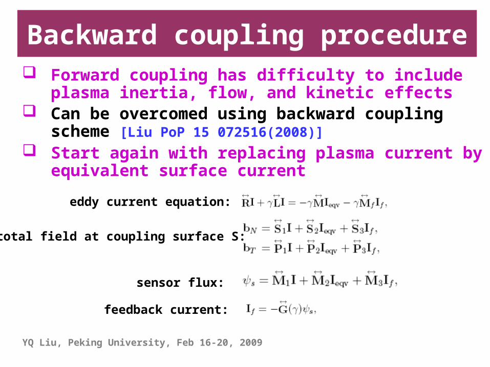
Forward coupling has difficulty to include plasma inertia, flow, and kinetic effects
Can be overcomed using backward coupling scheme [Liu PoP 15 072516(2008)]
Start again with replacing plasma current by equivalent surface current
Backward coupling procedure
eddy current equation:
total field at coupling surface S:
sensor flux:
feedback current:

YQ Liu, Peking University, Feb 16-20, 2009
With algebraic combinations of previous equations, it is possible to obtain the following linear relations (w.r.t. the eigenvalue)
Linear boundary condition for MHD code, with computational boundary at coupling surface
Sensor flux for RFA or feedback
Similar BC can be derived even for coupling to a nonlinear MHD code
Backward coupling procedure

YQ Liu, Peking University, Feb 16-20, 2009
Key features of CarMa Accurate for RWM calculations. Coupling scheme
analytically proven [Liu PoP 15 072516(2008)]. Well benchmarked against MARS-F for 2D walls, and against other similar codes for 3D walls
The coupling matrices assemble responses from all poloidal Fourier Harmonics. Hence the final system contains all unstable/stable RWM (multimode approach)
Capable of treating volumetric conductors (no thin shell approximations)
State-of-the-art fast techniques for solving EM problems allow very detailed modelling of conductor geometry [Rubinacci JCP 228 1562(2009)]
CarMa with backward coupling allows inclusion of inertia, rotation, kinetic effects, and feedback

YQ Liu, Peking University, Feb 16-20, 2009
Growth rate calculation Unstable eigenvalue of the dynamical matrix Standard routines (e.g. Matlab) or ad hoc computations
(e.g. inverse iteration: see the following…) Beta limit with 3D structures
Controller design state-space model (although with large dimensions and
with many unstable modes)
Time domain simulations Controller validation Inclusion of non-ideal power supplies (voltage/current
limitations, time delays, etc.)
What CarMa can do ?

YQ Liu, Peking University, Feb 16-20, 2009
Benchmark coupling scheme and CarMa
Choose a plasma with circular cross section, and aspect ratio =5
Assuming an axi-symmetric complete thin wall (2D wall), run MARS-F to compute growth/ damping rates of unstable/stable RWM
Run CarMa with 3D discretization of 2D wall
Compare results
q-profile
pressure profile

YQ Liu, Peking University, Feb 16-20, 2009
Both growth and damping rates agreeMARS-F [s-1] Coupling surface 1 [s-1] Coupling surface 2 [s-1]
Unstable eigenvalue 292.7 291.2 j 3.6e-4 293.3 j 7.5e-4
Stable eigenvalue #1 -165.7 -159.2 -159.3
Stable eigenvalue #2 -221.4 -216.6 -216.6
Stable eigenvalue #3 -279.4 -278.7 -278.2
Stable eigenvalue #4 -379.0 -373.9 -374.0
Stable eigenvalue #5 -560.5 -562.1 -561.3
Stable eigenvalue #6 -589.1 -581.2 -581.3
CarMa results independent of choice of coupling surface

YQ Liu, Peking University, Feb 16-20, 2009
Benchmark mode structure Eddy current density distribution along the wall,
computed by MARS-F alone (line) and by CarMa (circle)
For the unstable mode

YQ Liu, Peking University, Feb 16-20, 2009
Positive comparison with other 3D RWM codes (STARWALL, VALEN)
Courtesy of J. Bialek and
E. Strumberger
Benchmark with other codes

YQ Liu, Peking University, Feb 16-20, 2009
Outline1. Why important?
2. CarMa code
3. CarMa modelling and experiments RFX ITER
4. Outlook
5. Overall Summary (selected key notes)

YQ Liu, Peking University, Feb 16-20, 2009
RWM study for RFX: equlib. & geometry
RFX upgrade: rw=1.1a, R/a=2m/0.459m
Typical unstable RWM: m=1, |n|=2,...,6
•Coils•Mechanical structure•Vessel•Shell

YQ Liu, Peking University, Feb 16-20, 2009
RWM stability with MARS-F RWM growth rates are well measured in RFX experiments MARS-F with a 2D wall reproduces exp. growth rates for a large
range of plasma parameters and various n’s Including other structures tends to underestimate growth rates
MARS-F computes two unstable RWM for some n’s (=2,3)

YQ Liu, Peking University, Feb 16-20, 2009
RWM stability with CarMa (3D structure) For RFP plasmas, all three codes: ETAW(cylindrical
Newcomb solver), MARS-F, CarMa(2D) agree well, as shown below for one equilibrium
Gaps in conducting wall destabilize RWM. However, mechanical structures and outer shells give additional stabilization
3D wall structures (gaps) split two otherwise identical eigenvalues, as well as in tokamak cases
γ [s-1]
Cylinder(ETAW) MARS-F CarMa(2D) CarMa (3D)
n=2 <02.45
0.431.81
0.371.94
0.45, 0.462.40, 2.48
n=3 1.821.90
2.082.16
1.912.49
2.58, 2.622.96, 3.04
n=4 4.09 4.04 4.27 5.46, 5.53
n=5 6.81 6.89 7.45 9.62, 9.73
n=6 11.8 11.7 12.9 17.0, 17.2

YQ Liu, Peking University, Feb 16-20, 2009
3D effects are important on growth rate!
Purely axisymmetric estimates of growth rates are largely underestimated on RFX-mod
CarMa modelling vs. RFX experiments
Villone PRL 100 255005(2008)

YQ Liu, Peking University, Feb 16-20, 2009
Eddy current flow modified by wall gaps
2D wall
3D wall with gaps
CarMa computed wall eddy current pattern
For an unstable mode with n=3,m=1
YQ Liu, Peking University, Feb 16-20, 2009
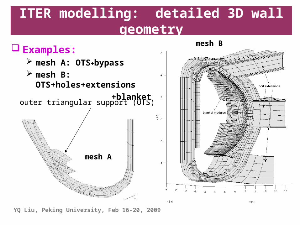
ITER modelling: detailed 3D wall geometry
Examples: mesh A: OTS+bypass mesh B:
OTS+holes+extensions +blanket
mesh A
outer triangular support (OTS)
mesh B

YQ Liu, Peking University, Feb 16-20, 2009
Simple hole approximation for ITER walls leads to too pessimistic prediction for RWM
stability Eddy current patterns significantly affected
by tubular extensions... that allow better imagine current flow, hence
more stablising effect

YQ Liu, Peking University, Feb 16-20, 2009
Major 3D wall effects are holes and tubular extenstions
3D holes roughly double growth rates Tubular extensions reduce growth rates to a
level as with 2D complete walls
γ [s-1 ] N 2.676 2.830 2.985 3.301 3.461
MARS-F γ 8.495 15.82 29.63 165.8 577.2
Mesh#1:2D γ 8.462 15.56 28.35 127.2 334.9
Mesh#2:2D+OTS γ 7.896 14.34 25.54 99.26 206.8
Mesh#3:2D+OTS+bypass γ 7.903 14.37 25.63 100.0 208.9
Mesh#4:3D+OTS+holes γ 15.83 32.60 71.94 N.A. N.A.
Mesh#5:mesh#4 refined γ 15.65 32.06 70.20 N.A. N.A.
Mesh#6:mesh#5 smaller holes γ 13.71 27.13 55.78 1230 N.A.
Mesh#7:3D+OTS+holes+ext. γ 9.366 17.63 33.22 184.4 878.7

YQ Liu, Peking University, Feb 16-20, 2009
RWM feedback study for new ITER in-vessel coils reveals requirement on the coil current
Consider an ITER plasma with Use 3x9 ELM control coils for RWM
feedback Multivariable controller based on LQG
technique satisfying certain specification requirements
N = 3.17
Actual limiting factor is current Assuming 20kA current
limit (ELM control off), RWM can be stabilised for field perturbation within 300Gauss
Assuming 250A current limit (ELM control on), field perturbation within 5Gauss
20kA current limit
1 sec. settling time

YQ Liu, Peking University, Feb 16-20, 2009
Detail: LQG controlMultivariable controller designed by
using the LQG technique, based on the following requirements
Obtain a closed loop null controllable region as close as possible to the ideal result (BAP)
Allow to recover from a disturbance (initial condition on the unstable plane) as soon as possible (within current/voltage limits)
Avoid to generate a n1 magnetic field
Stabilize all the modes with growth rates lower than reference equilibrium (i.e. lower N)
Use a balanced truncation technique to obtain a sufficiently low order controller (five)

YQ Liu, Peking University, Feb 16-20, 2009
Plasma/circuit model
V(t) y(t)TIN
TOUT
y1(t)
-
V1(t)
K(s)
27 input voltages (3 coils per 9 sectors)
3 voltage Fourier components
144 magnetic outputs
(48 measurements per 3 sectors)
48 magnetic Fourier
components
RWM feedback controller
Detail: control diagram

YQ Liu, Peking University, Feb 16-20, 2009
The BAP is in the range of perturbations of tens of mTThe BAP is in the range of
perturbations of fractions of mT
ELM control off: current limits 20 kAELM control on:
current limits 250 A
Bk(t) are N=18 measurements of the vertical magnetic field
in the outboard region at equally spaced toroidal angles
k
The interior of the polygon corresponds to stabilizable
perturbations
11
2cos
N
k kk
y t B tN
21
2sin
N
k kk
y t B tN
-0.04 -0.03 -0.02 -0.01 0 0.01 0.02 0.03 0.04
-0.03
-0.02
-0.01
0
0.01
0.02
0.03
y1 [T]
y 2 [T
]
-5 -4 -3 -2 -1 0 1 2 3 4 5
x 10-4
-4
-3
-2
-1
0
1
2
3
4
x 10-4
y1 [T]
y 2 [T
]
Another approach of control study: best achievable performasnce (BAP)

YQ Liu, Peking University, Feb 16-20, 2009
Control coils voltage-current distribution
40 80 120 160 200 240 280 320 360-3
-2
-1
0
1
2
3
Toroidal angle [deg]
Upp
er C
oil V
olta
ge [
V]
at t
=0
40 80 120 160 200 240 280 320 360-2.5
-2
-1.5
-1
-0.5
0
0.5
1
1.5
2
2.5
Toroidal angle [deg]M
id C
oil V
olta
ge [
V]
at t
=0
40 80 120 160 200 240 280 320 360-3
-2
-1
0
1
2
3
Toroidal angle [deg]
Low
er C
oil V
olta
ge [
V]
at t
=0
40 80 120 160 200 240 280 320 360-250
-200
-150
-100
-50
0
50
100
150
200
250
Toroidal angle [deg]
Upp
er C
oil C
urre
nt [
A]
at t
=0.
0075
s
40 80 120 160 200 240 280 320 360-200
-150
-100
-50
0
50
100
150
200
Toroidal angle [deg]
Mid
Coi
l Cur
rent
[A
]at
t=0.
0075
s
40 80 120 160 200 240 280 320 360-250
-200
-150
-100
-50
0
50
100
150
200
250
Toroidal angle [deg]
Low
er C
oil C
urre
nt [
A]
at t
=0.
0075
s

YQ Liu, Peking University, Feb 16-20, 2009
Outlook For RWM, geometrical coupling of different n’s
(including n=0!), via 3D conductors, is probably more important than physics coupling due to nonlinear MHD
Nonlinear MHD coupling should be more important for other, more localised modes such as TMs and ELMs
Extensive work going on to include 3D geometrical effects in RFA simulations RWM feedback stabilisation (in particular for ITER) Nonlinear (quasi-linear) MHD modelling for RWM (e.g.
nonlinear interplay between mode damping and momentum damping)

YQ Liu, Peking University, Feb 16-20, 2009
Overall summary (key notes)1. RWM research important for ITER
2. Sensor optimisation crucial for RWM feedback
3. Understanding RWM physics calls for hybrid MHD-kinetic description
4. RFA tests RWM damping physics
5. State-of-the-art in RWM modelling: Damping physics + 3D structures + feedback
