yig-sphere-based phase shifter for x-band phased array
TRANSCRIPT

San Jose State University San Jose State University
SJSU ScholarWorks SJSU ScholarWorks
Master's Theses Master's Theses and Graduate Research
Fall 2011
YIG-sphere-based phase shifter for X-band phased array YIG-sphere-based phase shifter for X-band phased array
applications applications
Donald C. Benson San Jose State University
Follow this and additional works at: https://scholarworks.sjsu.edu/etd_theses
Recommended Citation Recommended Citation Benson, Donald C., "YIG-sphere-based phase shifter for X-band phased array applications" (2011). Master's Theses. 4083. DOI: https://doi.org/10.31979/etd.p4je-rvaz https://scholarworks.sjsu.edu/etd_theses/4083
This Thesis is brought to you for free and open access by the Master's Theses and Graduate Research at SJSU ScholarWorks. It has been accepted for inclusion in Master's Theses by an authorized administrator of SJSU ScholarWorks. For more information, please contact [email protected].

YIG-SPHERE-BASED PHASE-SHIFTER FOR X-BAND PHASED ARRAY APPLICATIONS
A Thesis
Presented to
The Faculty of the Department of Electrical Engineering
San José State University
In Partial Fulfillment
of the Requirements for the Degree
Master of Science
by
Donald C. Benson
December 2011

© 2011
Donald C. Benson
ALL RIGHTS RESERVED
The Designated Thesis Committee Approves the Thesis Titled
YIG-SPHERE-BASED PHASE-SHIFTER FOR X-BAND PHASED
ARRAY APPLICATIONS
by
Donald C. Benson
APPROVED FOR THE DEPARTMENT OF ELECTRICAL ENGINEERING
SAN JOSÉ STATE UNIVERSITY
December 2011
Dr. Sotoudeh Hamedi-Hagh Department of Electrical Engineering
Dr. Masoud Mostafavi Department of Electrical Engineering
Dr. Raymond Kwok Department of Physics

ABSTRACT
YIG-SPHERE-BASED PHASE SHIFTER FOR X-BAND PHASED ARRAY APPLICATIONS
By Donald C. Benson
A novel technique for effecting phase shift of X-band signals has been developed
and analyzed for use with quadrature amplitude modulation (QAM) of signals in a phased
array application, and the impact of this phase shifter on error vector magnitude (EVM)
has been quantified. A commercially available filter consisting of yttrium iron garnet
(YIG) spheres was characterized by means of a network analyzer. The gain and phase
response was measured across a 25 MHz frequency band centered at 10 GHz, while the
filter was tuned in frequency steps such that a 360 range of phase shifts was achieved.
The S-parameters from these measurements were integrated with Matlab representations
of QAM-16 modulation, demodulation, and phased array antennas to model a complete
radio system. The EVM caused by non-ideal gain and phase response of the YIG filter
was determined for various beam angles and data patterns.
It was found that a YIG filter does provide stable phase shift suitable for phased
array applications, with acceptable attenuation so long as the frequency being transmitted
remains within the filter’s pass band. The particular filter analyzed did not contain
sufficient stages to maintain 3 dB flatness across the required 360 tuning range, but
performed satisfactorily for a limited range of beam orientation. The capability to provide
continuously variable phase shift offered by the YIG filter was found to not offer
significant advantage over the discrete steps produced by switched delay lines.

v
Table of Contents I. Introduction .......................................................................................................... 1
A. Background ....................................................................................................... 1
B. Related research ................................................................................................ 1
C. Selection of YIG sphere technology ................................................................. 3
II. Hypothesis ............................................................................................................ 8
III. Partition between hardware and mathematical simulation ................................... 9
IV. Implementation of YIG phase shifter ................................................................. 11
D. Design of a custom filter ................................................................................ 11
E. Selection of a commercial filter ..................................................................... 13
F. Characterization of filter ................................................................................. 14
V. The behavior of phased arrays ........................................................................... 22
VI. Simulation of radiation pattern ........................................................................... 24
VII. Simulation of modulation/demodulation and error vector magnitude ........... 28
G. Baseline model of digital radio with ideal channel ........................................ 28
H. Three-bit phase shifter for beam forming ....................................................... 39
I. Ideal Butterworth filter phase shifter for beam forming ................................ 40
J. Measured YIG filter phase shifter for beam forming ..................................... 44

vi
K. YIG filter phase shifter operated within -3 dB bandwidth ............................. 46
L. Swept beam angle using YIG filter phase shifter ........................................... 48
VIII. Issues identified in phased array systems ....................................................... 50
IX. Potential pitfalls of characterzation and analysis approach ............................... 52
X. On implementing an actual system .................................................................... 54
XI. Conclusion .......................................................................................................... 55
APPENDIX A. Matlab code ........................................................................................ 56
A. Radiation pattern ............................................................................................ 56
B. Antenna pattern .............................................................................................. 60
C. Constructive and destructive interference ...................................................... 61
D. Phase shifter .................................................................................................... 63
E. Digital radio model and EVM calculation ...................................................... 66
F. Idealized Butterworth beam former ................................................................ 84
G. Idealized Butterworth phase shifter ................................................................ 86
H. Recovery synchronization .............................................................................. 89
I. YIG beam former ........................................................................................... 93
J. YIG phase shifter ............................................................................................ 96
K. Swept beam angle ........................................................................................... 98

vii
L. Read S-parameter files and store in array ....................................................... 99
M. Read and plot filter S-parameter across entire passband .............................. 110
APPENDIX B. Data files ........................................................................................... 120
A. YIG S-parameter .......................................................................................... 120
References ....................................................................................................................... 128
viii
List of Figures
Figure 1. Schematic representation of YIG bandpass filter 3
Figure 2. Original concept of bi‐directional system 5
Figure 3. Transformation of impedance through stages of a filter 11
Figure 4. YIG filter 13
Figure 5. S‐parameter test setup 15
Figure 6. 2 ‐ 20 GHz response of YIG filter 17
Figure 7. Measured gain and phase of YIG filter across the pass band 18
Figure 8. Measured gain and phase of YIG filter across frequency band of radio 20
Figure 9. Phase shift vs. beam angle 22
Figure 10. Radiation pattern with ideal phase shifters 25
Figure 11. Radiation pattern with 3‐bit phase shifters 26
Figure 12. Radiation pattern with YIG phase shifters 26
Figure 13. Constellation and I/Q modulation of [56A9401237BFEDC8] 33
Figure 14. QAM‐16 modulation and frequency content of [56A9401237BFEDC8] 34
Figure 15. Recovered constellation, I & Q, and error for [56A9401237BFEDC8] 36
Figure 16. Constellation and I/Q modulation of [0F4B87C3D2E1A569] 37
Figure 17. QAM‐16 modulation and frequency content of [0F4B87C3D2E1A569] 38
Figure 18. Recovered constellation, I & Q, and error for [0F4B87C3D2E1A569] 39
Figure 19. Recovered constellation, I & Q, and error, 3‐bit phase shifter 40

ix
Figure 20. Butterworth bandpass filter tuned around 10 GHz to provide phase shift 41
Figure 21. Recovered constellation, I & Q, and error, Butterworth phase shifter 43
Figure 22. Recovered constellation and delta error YIG vs. baseline 45
Figure 23. Recovered constellation and delta error YIG vs. baseline for small angle 47
Figure 24. EVM variation as beam swept from 0 to +90 by YIG phase shifter 49

x
List of Tables
TABLE I. I and Q encoding of symbols 30

1
I. INTRODUCTION
A. Background
Passive technologies used to provide continuously variable phase shift for lower
frequencies up to a few gigahertz, such as LC filters tuned with varactor diodes, do not
meet the needs of operation in the 10 GHz X-band region. Alternatives such as switched
delay lines offer only discrete steps in delay, while active monolithic microwave
integrated circuit (MMIC) devices used to generate signals for each antenna element add
complexity and cost. Custom thin-film yttrium iron garnet (YIG) phase shifters have also
been an area of research. YIG filters and resonators such as those offered by Microlambda
Wireless [1] have been used for other applications in communication and test equipment.
B. Related research
Technologies used to provide continuously variable phase shift for lower frequencies
up to a few gigahertz do not function at X-band frequencies (8.2 to 12.4 GHz). YIG thin
films and YIG slabs have been used to provide adjustable propagation delays for signals
carried by microstrip or stripline transmission lines operating at such frequencies. They
have also been used to provide delayed coupling between parallel transmission lines
placed over the YIG material. Demidov et al. [2] described the use of yttrium-iron-garnet
(YIG) films grown on substrates of suitable lattice dimensions, especially gadolinium-
gallium-garnet (GGG), as a tunable magnetic medium for phase shifters. With this
material placed over microstrips, the propagation delay of electromagnetic waves could be
varied with an externally applied magnetic field. How et al. [3] noted that operating

2
frequency had to be well away from the resonant frequency the YIG was tuned to or the
losses would be high. That tendency to dissipate energy at resonance is similar to having
a high frequency decoupling capacitor (a deliberately fabricated capacitor in series with
parasitic inductance), which serves to absorb energy at its resonant frequency. The same
behavior can also be obtained with a discrete inductor and capacitor. Either way, this
circuit may be used to reduce noise such as harmonics from a digital system that affects
radio reception. However, such attenuation is undesirable when shifting the phase of a
signal.
Tatarenko et al. [4] described phase shifters using the characteristic of YIG that it
rotates the orientation of a magnetic field at its resonant frequency. The design described
took advantage of this behavior with two orthogonal microstrips placed over a YIG disc.
YIG-tuned filters utilizing the same behavior, which permits precision control based on a
tunable resonant frequency, are similarly constructed by placing two orthogonal loops of
wire around a YIG sphere (see Fig. 1).

3
Figure 1. Schematic representation of YIG bandpass filter
In this configuration the YIG implements a transformer with behavior similar to an
LC bandpass filter with Q=1000. At the resonant frequency, rather than dissipating the
input energy, the circuit couples it effectively to the output. The use of a YIG disc as a
phase shifter is the closest to the work described in this thesis, as there are no known
reports of YIG spheres used as phase shifters.
Finally, Foster et al. [5] described using water-cooled slabs of YIG in a waveguide to
provide adjustable timing of a 2MW signal used in a particle accelerator.
C. Selection of YIG sphere technology
Phase shifters based on YIG spheres were selected for study based on apparent
advantages over other technologies.
4
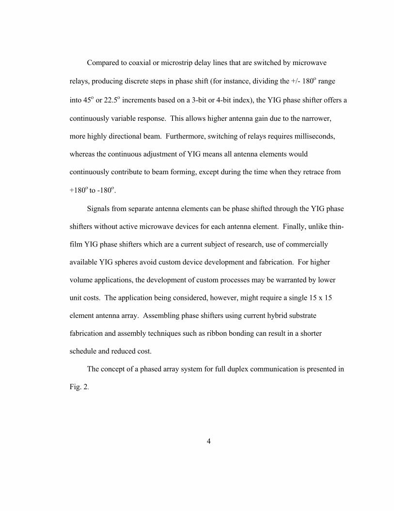
Compared to coaxial or microstrip delay lines that are switched by microwave
relays, producing discrete steps in phase shift (for instance, dividing the +/- 180 range
into 45 or 22.5 increments based on a 3-bit or 4-bit index), the YIG phase shifter offers a
continuously variable response. This allows higher antenna gain due to the narrower,
more highly directional beam. Furthermore, switching of relays requires milliseconds,
whereas the continuous adjustment of YIG means all antenna elements would
continuously contribute to beam forming, except during the time when they retrace from
+180to -180.
Signals from separate antenna elements can be phase shifted through the YIG phase
shifters without active microwave devices for each antenna element. Finally, unlike thin-
film YIG phase shifters which are a current subject of research, use of commercially
available YIG spheres avoid custom device development and fabrication. For higher
volume applications, the development of custom processes may be warranted by lower
unit costs. The application being considered, however, might require a single 15 x 15
element antenna array. Assembling phase shifters using current hybrid substrate
fabrication and assembly techniques such as ribbon bonding can result in a shorter
schedule and reduced cost.
The concept of a phased array system for full duplex communication is presented in
Fig. 2.

5
Figure 2. Original concept of bi-directional system
A bit stream of hexadecimal symbols (0 through F) is modulated as QAM-16
constellations, with two bits selecting a row and two bits selecting a column in the
constellation. The X-axis, referred to as I, modulates the amplitude of a sinusoidal signal
while the Y-axis, referred to as Q, modulates the amplitude of another sinusoidal signal
that is 90 out of phase with the first one. When these two amplitude-modulated signals
are summed, the result is an amplitude and phase-modulated signal. Although this signal
has a single frequency with constant amplitude and phase, the transition between

6
modulated symbols introduces other frequency components of varying amplitudes. The
frequency envelope shown represents what might be present in a long string of symbols
(after filtering to remove the infinite number of higher harmonics generated by the abrupt
change between symbols). This signal, referred to as intermediate frequency (IF), is then
multiplied with the signal from a local oscillator (LO) by means of a non-linear
component called a mixer. The resultant frequency spectrum includes all frequencies
coming from (1) where n and m are all positive integers.
After filtering to remove the undesired images, the RF signal contains the
transmitted information centered about the carrier frequency, which is the sum of LO and
IF frequencies.
After amplification, the RF signal is split and sent through phase shifters to the
antenna elements. Each phase shifter is directed to introduce a delay or phase shift, such
that the transmitted signal will be in phase with signals from other antenna elements when
they are the same distance from the desired target.
For the receive path, after phase shifting the signals that arrived at the antenna
elements at different times so they constructively interfere (i.e., add linearly because they
are in phase), the signals are summed and directed to the demodulation circuitry. The
received RF is multiplied by LO and the desired IF from (2) is filtered out.

7
The IF is then sampled and multiplied by two sinusoids 90 out of phase with each
other (and suitably synchronized in phase with the IF signal) to recover I and Q values.
Due to errors in the system such as undesired frequency-dependent attenuation or phase
shift, these values will not be precisely the ones sent. The nearest allowable value is
selected, and so long as the error is less than 50% of the difference between levels
representing adjacent points in the constellation, the data can be recovered without error.
The deviation from ideal values is Error Vector Magnitude, a key metric of channel
quality.
As originally conceived, the YIG filter would be used as a phase shifter in a bi-
directional digital radio system, with only passive elements (the phase shifters and
splitter/combiners) between the power amplifier (PA)/low noise amplifier (LNA) and the
antenna, as shown in Fig. 2. The idea for this architecture was based on some literature
that suggested each sphere could transfer as much as 2W of power. However,
specifications for some commercially available YIG band pass filters showed only 10 mW
of power handling capability [1]. A commercially built filter was subjected to a power
sweep from -50 dBm to +20 dBm (100 mW is the maximum output available from the
Agilent E8364B VNA) at 10.0 GHz, and no compression was observed. Further testing
with an external amplifier would be required to measure the response at higher power. If
not able to handle at least 1W, without the addition of power amplifiers for each antenna
element, this technology is appropriate only for receiver (but not transmitter) applications,
such as gathering telemetry data.

8
II. HYPOTHESIS
Several technologies are currently used for phase shifters. One type is based on
varactor diodes, which provide a continuously variable capacitance when bias voltage is
changed. Varactor phase shifters are capable of operating up to the low gigahertz
frequency range but are not suitable for X-band. Another type that is used for X-band has
relays to switch between fixed delay lines of different lengths. Switched delay line phase
shifters provide very flat gain response but offer adjustment only in discrete steps and
carry no power during the switching transition. A third type currently used for phased
arrays at X-band frequencies and higher is based on monolithic microwave-integrated
circuit (MMIC) technology. MMIC phase shifters vary the amplitude of sine and cosine
signals to provide a continuously adjustable phase shift.
A band-pass filter based on YIG spheres will provide precise phase shift, with
acceptable variation in attenuation, resulting in higher gain of a phased array antenna
system operating at X-band microwave frequencies compared to discrete delay lines. The
continuously variable response will permit rapid sweeping of beam direction without loss
of power to antenna elements due to switching. The ability to provide phase-shift without
active microwave devices for each antenna will permit a lower-cost implementation.

9
III. PARTITION BETWEEN HARDWARE AND MATHEMATICAL SIMULATION
In order to show the impact of YIG phase shifters on total system performance, a
physical YIG phase shifter was characterized on a network analyzer and the rest of the
communication system was modeled as idealized elements in Matlab. A typical system
would use a two-dimensional antenna array to direct the beam in elevation as well as
azimuth. To simplify bookkeeping within the simulation and graphical representation of
radiation patterns a one-dimensional array was modeled. A real system would use patch
antennas because they are appropriate to support beam-forming in two dimensions. The
idealized Hertzian dipole was used for this study. Three-dimensional equations for the
Hertzian dipole were used, and the three-dimensional radiation pattern was reviewed
graphically for validity.
Initially an idealized phase shifter was modeled. This was compared to simulation
of an ideal Butterworth bandpass filter (as representative of an ideal YIG filter), a
simulation of 3-bit (45 increment) phase shifters consisting of coaxial cables (a typical
phase shifter used in microwave applications), and finally captured S-parameters from the
YIG phase shifter.
To make the Butterworth filter tunable for phase shift, it was parameterized such that
values were computed according to center frequency, and the center frequency was
selected based on desired phase shift. Similarly, an array of measured YIG phase shifter
S-parameters generated at various magnetic field intensities was used to generate the
response for each element. Initially linear interpolation was considered, but 10

10
increments were found to be close enough to ideal, so the measured S-parameter with
phase shift closest to the desired value was used without interpolation.
11
IV. IMPLEMENTATION OF YIG PHASE SHIFTER
D. Design of a custom filter
The original plan was to fabricate a filter with the desired characteristics. A phase
shifter capable of 360 phase shift is necessary to support even limited pointing angles
(less than 180) with a large number of elements spanning a distance much larger than one
wavelength. Review of commercially available YIG bandpass filters showed that a filter
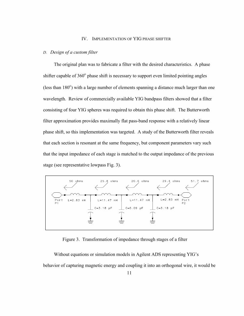
consisting of four YIG spheres was required to obtain this phase shift. The Butterworth
filter approximation provides maximally flat pass-band response with a relatively linear
phase shift, so this implementation was targeted. A study of the Butterworth filter reveals
that each section is resonant at the same frequency, but component parameters vary such
that the input impedance of each stage is matched to the output impedance of the previous
stage (see representative lowpass Fig. 3).
Figure 3. Transformation of impedance through stages of a filter
Without equations or simulation models in Agilent ADS representing YIG’s
behavior of capturing magnetic energy and coupling it into an orthogonal wire, it would be

12
necessary to devise a method to appropriately determine dimensions for a prototype.
Although this unique behavior was not available as a model parameter in ADS, magnetic
permeability is a standard material parameter. The approach that would be taken is to
select dimensions of the wire loop such that with the sphere inside, impedance of 50_
would be maintained. The orthogonal wire loop dimensions would be set to achieve the
desired output impedance for the first stage, and dimensions of other stages would be
determined in a similar manner to maintain impedance match between stages.
The physical implementation initially conceived was to design a hybrid substrate
with appropriate dielectric such as Teflon. Various low-temperature co-fired ceramics
(LTCC) would also be appropriate, but prototype techniques and shrinkage issues make
these more difficult than etching of a double-sided laminate. Interconnect between each
stage would be designed to match the targeted impedance. Metalization supporting gold
wirebonding would be required. Loops were to be formed with a ribbon bonder,
providing interconnect with a wide cross-section for low resistive losses. SMA connectors
would be soldered to the substrate.
Further investigation revealed that tuning of a multi-stage YIG filter is a relatively
involved process. Resonant frequency and input and output impedances of each stage
must be correct, as with any multi-stage filter. However, the degrees of freedom to be
adjusted for a YIG filter are not just loop area and sphere location; the spheres themselves
must be binned for desired characteristics [6]. This made such an implementation beyond

13
the scope of this project. Accordingly, a commercially available YIG filter was
characterized.
E. Selection of a commercial filter
Due to the difficulty of fabricating a YIG filter with sufficient performance, a
commercially available YIG filter from Yig Tek was obtained, model number 183-43 (see
Fig. 4).
Figure 4. YIG filter

14
F. Characterization of filter
For actual usage it is necessary to stabilize the temperature of the YIG sphere.
Variations in ambient temperature, and variations in self-heating depending on RF power,
would cause a drift in response. By heating the YIG sphere to a regulated temperature RF
performance can be measured and recorded as calibration data correlating tuning current
with frequency.
According to Bryant et al. [7], “Heating to 105 C +/- 5 gives approximately seven
fold reduction in changes due to temperature variation.” This is one of the techniques that
gives YIG sphere based oscillators the frequency stability required for use as a time base
in microwave test equipment such as Vector Network Analyzers (VNA) and Spectrum
Analyzers. The commercially available YIG filter which was characterized has an
internally regulated heater for this purpose. With variation of temperature reduced, only
regulation of current used to generate the magnetic field is necessary to set resonant
frequency, and the YIG filter operates with stable phase shift. For the purpose of this
work, the YIG filter was permitted to stabilize at operating temperature and measurements
were performed with steady state (or repeatedly swept) RF power, so the heater was not
required.
Characterization was performed with an Agilent E8364B 50 GHz Vector Network
Analyzer (VNA), connected to the YIG filter with Gore cables and 2.4mm to SMA
adapters (see Fig. 5).

15
Figure 5. S-parameter test setup
Bias current for the electromagnet was provide by two Agilent E3630A +6V, +/-20V
power supplies. A regulated current source should be used, but none was readily
available, so a series resistor was used instead to set a current from the voltage source. To
achieve sufficient resolution to allow tuning of the filter phase shift in 10 increments (+/-
3), the supplies were connected in series to provide 46V. The YIG filter tuning coil has
nominal 6 DC resistance, and two, 50 10W resistors were connected in series.
Resolution of the control for the power supply output voltage was the limiting factor in
adjusting frequency and phase shift of the filter. Current ranging from 380 mA to 420 mA
spanned the desired tuning range, but only a slight nudge to the control knob changed
phase by more than 10. A circuit utilizing a 10-turn potentiometer or digital control

16
would have been easier to use. At any given setting, however, the response was stable;
phase jitter was only 0.4 and gain jitter was only 0.05 dB with the network analyzer’s
averaging function turned off. Averaging was turned on for calibration and data
gathering. The addition of a 2.5 K potentiometer in parallel with the YIG filter’s tuning
coil allowed adjusting the response with sufficient resolution to easily select the desired
10 increments.
An attempt was made to determine power handling of the filter by sweeping power
from -50 dBm to +20 dBm (100 mW, which is the maximum VNA output), but no gain
compression was observed. An external power amplifier (PA) would be required to find
the capability of this filter.
Frequency sweeps were taken at 0 dBm RF power and various magnetic field
strengths producing a phase shift (at 10 GHz) of -180 to +180 in 10 steps; the data from
these 36 frequency sweeps were stored as S-parameter files. Frequency steps are typically
linear or logarithmic when generated by test equipment, unlike electromagnetic field
solvers that may increase resolution depending on simulated response. If captured (or
modeled) S-parameter files are used in a subsequent simulation that includes frequency
points not in the data, interpolation must be performed to estimate the response at those
particular frequencies. To avoid interpolation errors, frequency steps on the VNA were
selected to match those used for Fourier analysis of the simulated signal; no interpolation
was required.

17
Also, steps in magnetic field strength were selected so the phase shift was in small
enough steps to be used directly for beam forming. With 10 increments, the greatest
variation from desired angle would be 5; cos(5) is 0.996, so this approximation
contributed only 0.4% variation in resultant signal strength.
A sweep of the entire 2 - 20 GHz range of the filter is shown in Fig. 6.
Figure 6. 2 - 20 GHz response of YIG filter
The bandpass response was measured as S-parameters over the frequency range 9.9 -
10.1 GHz and shows the YIG filter’s 50 MHz bandwidth at -3 dB. Five representative

18
sweeps were taken to demonstrate how tuning moves the -3 dB cutoff points as it shifts
the phase (see Fig. 7).
Figure 7. Measured gain and phase of YIG filter across the pass band

19
It is clear from this plot that shifting the center 10 GHz frequency from a -180 to
+180 phase shift will cause greater than the desired 3 dB attenuation. The YIG filter
selected is not a high enough order filter (i.e., does not have enough YIG sphere stages) to
provide the desired phase shift. The radio bandwidth used in this study, 25 MHz, is
relatively narrow. Still, at +/- 12.5 MHz from the center frequency, the attenuation is
greater. Calculations of the impact on this attenuation on radio performance were made
for two situations – one with arbitrary beam angles, utilizing the larger phase shifts
(resulting in undesirable attenuation), and again with a small angle where the required
phase shifts can be accomplished with no more than 3 dB of attenuation. The latter
calculation is representative of performance available from a YIG filter with greater
bandwidth.
In the plot of gain, there is a ripple in the pass band. This was at first thought to be
caused by adapters used between 2.4 mm test ports and SMA connectors on the YIG filter
because their physical length was close to the wavelength in question. However, it can be
seen in this plot that the ripple changes frequency as the filter is tuned. It is part of the
tunable filter itself and not part of the fixed hardware.
S-parameter measurements were taken with a frequency sweep consisting of 51
uniformly spaced points from 9.98779 GHz to 10.01220 GHz, precisely matching the
(lowest 25 MHz bandwidth) up-converted frequency points produced by Fast Fourier
Transform (FFT) of the data stream. The filter was tuned to produce 10 increments of
phase shift and data gathered at each of 36 settings (see Fig. 8).

20
Figure 8. Measured gain and phase of YIG filter across frequency band of radio
The phase for some crossed over from -180 to +180, as expected. The ripple
shown in phase was undesirable; this non-linearity in phase response over frequency was

21
one of the sources of distortion in the modulated data. Some of the gain waveforms also
showed a ripple, coincident with the phase ripple.
For use as a phase shifter, it was desired to achieve a phase shift of +/- 180 for the
nominal 10 GHz operating frequency and maintain gain flatness within 3dB across a 25
MHz bandwidth centered at nominal. For some of the tuned phase shifts, this filter
produced a gain output ranging from -10 dB down to -21 dB. The significance of the
reduced gain is that antenna elements fed with that signal received power -6 dB (1/4
power) or lower compared to the other elements, and therefore did not contribute
appreciably to the transmitted wavefront. For a receiver application, only 1/4 or less of
the power received by that element was utilized. In either transmit or receive applications,
the attenuation reduced signal strength and directionality.
The available phase shifts with no more than 3 dB additional attenuation (in addition
to the peak -2.6 dB response) were from +60 to +180 (+180 and -180 being the same).
In order to show the radio performance with a YIG phase shifter that provides the desired
bandwidth and phase shift, modeling was performed utilizing this limited range, which
provides 120 of adjustment in phase shift, or 0.333 lambda. An antenna array with 15
elements separated by 1.0 lambda, with 120 of adjustment in phase shift, can sweep
through a 1.27 angle. While this angle is small and the beam may not appear different
from one generated by antenna elements that are in phase, this calculation does
incorporate the frequency-dependent attenuation of the YIG filter within the pass band.

22
V. THE BEHAVIOR OF PHASED ARRAYS
Phased array antennas provide increased transmitted signal strength (or receive
sensitivity) by introducing a phase shift between signals to or from each antenna element
so the waves will have constructive interference in the desired direction due to alignment
of phase as shown in Fig. 9.
Figure 9. Phase shift vs. beam angle

23
This also causes reduced signal strength (or sensitivity) in other directions.
However, there are many smaller lobes of increased signal strength in the radiation pattern
at angles other than the desired beam direction where some of the waves again arrive in
phase and cause constructive interference. Where the waves interfere destructively the
signal strength is reduced. The total energy transmitted is the sum of what each antenna
emits, but more of it is delivered in the beam direction. The ratio of peak energy (in the
beam direction) to what would be delivered by a spherical radiator that delivered equal
energy in all directions is referred to as “gain” of the antenna.
24
VI. SIMULATION OF RADIATION PATTERN
A notional phased array antenna system was described in Matlab. It was
implemented as a one-dimensional array of elements. The constructive and destructive
effects of waves propagating from each element were combined to produce a three-
dimensional model. The phase-shifted signal produced by each antenna element was
further shifted according to (3) and then added to the wavefront produced by the other
antenna elements.
_ e _
(All dimensions were described in terms of wavelength or , and phase angles
which are the same as t were used to compute changes to the waveform.) Equation (4)
from Ulaby [6] describing the three-dimensional radiation pattern of a Hertzian dipole was
then multiplied by this model, generating the radiation pattern for the entire phased array
system.
F θ, φ sin θ
This analysis was limited to Continuous Wave (CW) signals, a pure sine wave at the
carrier frequency. The radiation pattern may differ at other frequencies within the radio
system bandwidth about the carrier frequency due to non-idealities of the phase shifter;
this is addressed by analysis of the distortion in modulated signals, which are affected by
differences in both amplitude and phase between frequency components of the signal.
Using this approach, beam forming with various phase shifters was compared. In

25
particular, the relative gain for an ideal (perfect) phase shifter (see Fig. 10), a 3-bit delay
line phase shifter (see Fig. 11), and a YIG phase shifter (see Fig. 12) were compared.
Figure 10. Radiation pattern with ideal phase shifters
Note that due to symmetry, there is a beam formed “behind” the antenna array
mirroring the beam in front.
26
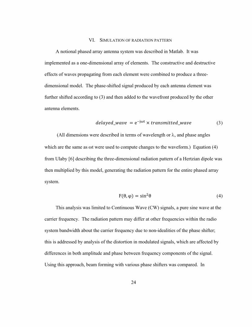
Figure 11. Radiation pattern with 3-bit phase shifters
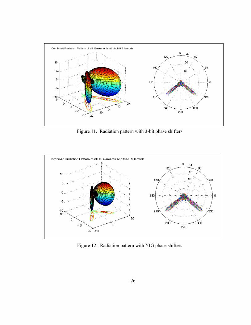
Figure 12. Radiation pattern with YIG phase shifters

27
With an ideal phase shifter, the beam produced at a 40 angle from an array of 15
antenna elements showed gain of 22.5, which means the field strength at the point of
strongest field was 22.5 times what an omni-directional radiator would produce. This is
the expectation for the perfect case; 15 elements in perfect phase multiplied by the 1.5
gain of the Hertzian dipole.
When a 3-bit (45) phase shifter was used instead, the gain was 21.9, so the penalty
for adjusting phase in these larger increments was only 3%. This shows that part of the
hypothesis of this project, that precise control of phase shift would provide a more
directional beam than is possible with fixed delay lines, is not correct. YIG may still offer
a benefit in tuning speed, however.
With the YIG phase shifter, the gain was just 16.8. This was not due to error in
phase shift, but rather due to attenuation when the phase shifter was used outside its pass
band. The response of the S-parameters was normalized to 0 dB at the center of the pass
band to represent an amplifier restoring the lost signal strength, but for some phase shifts
the signal was attenuated by a considerable amount. If a higher order filter with sufficient
bandwidth had been used, all antenna elements would have received a signal between 0
dB and -3 dB so the gain would have improved, but still below that of the lossless ideal or
3-bit delay line based phase shifter designs.
28
VII. SIMULATION OF MODULATION/DEMODULATION AND ERROR VECTOR MAGNITUDE
A perfectly formed phased array system with ideal delay lines feeding each element,
or a dish antenna, would deliver modulated and up-converted signals without further
distortion except for group delay resulting from propagation through the atmospheric
medium. With any physical realization of phase shifters, however, additional group delay
and frequency dependent attenuation is introduced. This issue is the primary focus of the
work presented here.
G. Baseline model of digital radio with ideal channel
First, a baseline model was created in Matlab. The order of modulation and bit
stream length was selected for convenience of simulation and presentation. The
modulation was QAM-16, and a bit stream 16 symbols long was simulated. Higher order
modulation would likely be used for high data rates in practical systems. However,
techniques to reduce inter-symbol interference could be required. For this work, the lower
order modulation permitted the bit stream to be recovered and EVM quantified. Then, the
additional EVM resulting from a different channel (in this case imperfect phase shifters)
could be determined. Likewise, the bit stream length selected was relatively short so
resultant modulated waveforms could be easily presented. Longer bit streams provide all
possible cases of inter-symbol interference, for instance 220 bits which might be used on a
Bit Error Rate (BERT) tester that operates with hardware running at full channel speed.
With a large number of bits and the actual non-ideal behavior of a system, a constellation
diagram for the modulated data shows blurring of spots, a graphical representation of

29
EVM. Using a string of just 16 symbols and the repeatability of mathematical modeling,
each symbol was recovered as a single I/Q value, and these errors were combined by
Root-Sum-Square (RSS) to generate an EVM. Predictably, “easy” bit streams with small
changes in I and Q values produced lower EVM, and “hard” bit streams with large jumps
in I and Q values produced higher EVM.
QAM-16 modulation is represented as 16 points, in a 4x4 array, and encodes 24 or
16 bits represented in hexadecimal as 0, 1, 2, 3, 4, 5, 6, 7, 8, 9, A, B, C, D, E, F. To
modulate the data, each symbol is separated into the low two bits, which index into the X
or I axis of the modulation, and the high two bits, which index into the Y or Q axis. For
instance, “B” is “0111” in binary, so the low bits “11” designate the rightmost column of
the 4x4 array, and the high bits “01” second row from the bottom. The I and Q values
were then converted to a gain factor (to multiply with a 1.0V signal) centered at 0.0, so
“00” would be represented as -1.5V, “01” as -0.5V, “10” as +0.5V, and “11” as +1.5V.
(see TABLE I. )

30
TABLE I. I AND Q ENCODING OF SYMBOLS
+1.5 11
C
(1100)
D
(1101)
E
(1110)
F
(1111)
+0.5 10
8
(1000)
9
(1001)
A
(1010)
B
(1011)
Q ‐0.5 01
4
(0100)
5
(0101)
6
(0110)
7
(0111)
‐1.5 00
0
(0000)
1
(0001)
2
(0010)
3
(0011)
00 01 10 11
‐1.5 ‐0.5 +0.5 +1.5
I
A time-domain representation of 12.5 MHz 1.0V sine and cosine signals was
created, with 20 data points per cycle as the un-modulated baseband signal. The I and Q
representations of each bit were used to scale a single cycle of the signal, which were then
added together and concatenated with the waveform representing the next cycle. The data
rate was therefore 4 bits x 12.5 MHz or 50 Mbps. Because it was recognized that the sine
wave used for I modulation would switch between symbols when crossing zero volts,
while the cosine wave for Q modulation would switch at maximum value, both were offset
by 45 to balance the amount of high-frequency energy generated in each. Rather than
31
one having a value of 0.0V and the other having a value of 1.0V at the point in the
waveform where amplitude is changed, each has a value of 0.707V. (An even better
approach might have been to delay the Q part of the symbol by 45 so both switch at 0.0V.
While that would eliminate voltage discontinuities in the modulated signal, the derivatives
would still be undefined, so energy in frequencies outside the channel bandwidth could
not be completely eliminated.) An FFT (Fast Fourier Transform) was then performed to
generate a frequency-domain representation of the time-domain modulated signal.
The modulated signal was treated as having been up-converted to the target 10 GHz
X-band frequency. A physical mixer used for this purpose would necessarily introduce
distortions in-band from third-order harmonics, but as a model of an ideal mixer, the time
axis of the FFT data was simply changed.
To check behavior of the model, the data was converted back to baseband, assuming
the channel had unlimited bandwidth. That is to say, all frequency components in the FFT
data were used to recover the time-domain modulated data, and it was subsequently
demodulated. The I and Q components reproduced the input bit stream and had errors on
the order of 10-15, representing only mathematical rounding errors. The frequency data
was then truncated beyond 25 MHz bandwidth with an idealized brick wall filter. The
data was still recoverable, but this time EVM ranging from 6.8% to 35.9% resulted
depending on the bit stream. This was used as a baseline for comparison with non-ideal
channels representing phase shifters and the summing of wave-fronts from them.

32
While it is readily apparent that the distortion produced by the bandwidth-limited
idealized channel would be too high to support reliable communication at higher symbol
rates or with higher order modulation like QAM-64 or above, because the same magnitude
error would represent a higher portion of the inter-symbol spacing, normal design
techniques would reduce the distortion. In particular, the abrupt transitions in I and Q
values could be digitally filtered to reduce high frequency content, and the final level
could be adjusted to compensate depending on the previous symbol. This could be
performed either before transmission or after reception. Only the additional error
introduced by the phase shifter should be considered representative of an actual system,
and not that of the modeled communication system used as a baseline.
One bit stream what was tested was [56A9401237BFEDC8], which was selected
because the magnitude of transitions is minimized, and the order of bits as displayed in the
modulation constellation is easy to follow (see Fig. 13). It has minimum high-frequency
content, and is useful as an example because the bit sequence can be matched to graphical
representations of the I and Q bit stream.

33
Figure 13. Constellation and I/Q modulation of [56A9401237BFEDC8]
The resultant QAM-16 modulation, RF frequency content of baseband, and a 25
MHz low pass filter (applied to the baseband, but equally representative of a band-pass
filter from 9.9875 GHz to 10.0125 GHz applied after mixing with LO to shift the signal up
to X-band) are shown in Fig. 14.

34
Figure 14. QAM-16 modulation and frequency content of [56A9401237BFEDC8]
The abscissa of each graph is points in the data array – 320 samples for the time-
domain waveform, and 512 frequency points from an FFT computed on it. Note that data
generated by Matlab includes both positive and negative frequencies, but instead of
placing negative frequencies to the left of zero (which represents DC), the negative
frequencies are presented to the right of the highest positive frequency. The 26th point in
the frequency array, above which the brick wall filter cut off output, was at 24.9 MHz in
the baseband. For the link bandwidth to be made wider it would be necessary to increase
the baseband frequency. Because 12.5 MHz was selected, with a local oscillator (LO)
frequency of 9.9875 GHz, the modulated data is centered at 10.0 GHz (5), but also
replicated at 9.9750 GHz (6); if bandwidth greater than +/- 12.5 MHz from baseband was
permitted into the mixer these two would overlap.

35
Recovery of modulated data requires synchronization with the timing of symbols in
the signal. For amplitude modulation, it also requires proper adjustment of gain. Actual
implementation of a system would use a phase-locked loop (PLL) to synchronize the
signals used for down-converting and demodulation. For this analysis delay was manually
added so demodulation is synchronized with transitions in the bit stream. Otherwise, each
symbol would be incorrectly recovered as a combination of levels taken from two adjacent
symbols. Similarly, phase shift associated with the delay would interfere with recovery of
I and Q within the symbol.
The received baseband signal was separated into time slices the length of a single
symbol. Each was then multiplied by sine and cosine waves and the mean computed,
recovering the levels of the respective I and Q signals (see Fig. 15).
36
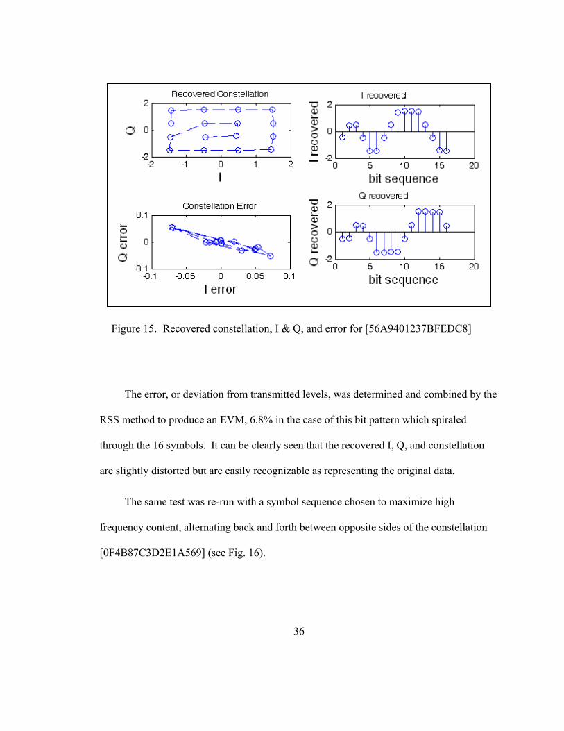
Figure 15. Recovered constellation, I & Q, and error for [56A9401237BFEDC8]
The error, or deviation from transmitted levels, was determined and combined by the
RSS method to produce an EVM, 6.8% in the case of this bit pattern which spiraled
through the 16 symbols. It can be clearly seen that the recovered I, Q, and constellation
are slightly distorted but are easily recognizable as representing the original data.
The same test was re-run with a symbol sequence chosen to maximize high
frequency content, alternating back and forth between opposite sides of the constellation
[0F4B87C3D2E1A569] (see Fig. 16).

37
Figure 16. Constellation and I/Q modulation of [0F4B87C3D2E1A569]
The resultant QAM-16 modulation and frequency content are shown in Fig. 17.
Significantly more high frequency content is seen as expected. The frequency content lost
due to 25 MHz channel bandwidth is presented in red, while the preserved content is
presented in blue.

38
Figure 17. QAM-16 modulation and frequency content of [0F4B87C3D2E1A569]
The recovered constellation and I & Q data shown in Fig. 18 have significantly more
distortion as is to be expected due to the greater amount of high-frequency information
which is outside the bandwidth-limited channel.

39
Figure 18. Recovered constellation, I & Q, and error for [0F4B87C3D2E1A569]
This time the EVM is 35.9% (providing 37.5 MHz bandwidth would reduce it to
19.3%). Because the maximum error in the constellation is less than 0.5 (half the
separation between symbols) in both I and Q, 100% of the data is recovered correctly.
H. Three-bit phase shifter for beam forming
The simulation was repeated for the symbol sequence [0F4B87C3D2E1A569], this
time utilizing the 3-bit (45 increment) phase shifter (See Fig. 19) .

40
Figure 19. Recovered constellation, I & Q, and error, 3-bit phase shifter
The EVM was again 35.9%. Note that the delay line model used was lossless and
introduced no distortion due to group delay; it represented ideal switches and transmission
lines.
I. Ideal Butterworth filter phase shifter for beam forming
Prior to measuring an actual phase shifter, a Matlab model of an idealized phase
shifter was developed based on the Butterworth approximation. Eighth-order high-pass
and low-pass filters were combined. The transfer functions for cutoff frequency of 1
radian/second were given by (7) for lowpass and (8) for highpass.
. . . .

41
. . . .
For zero phase shift, the highpass was set to provide a low frequency cutoff of 6.67
GHz, and the lowpass was set to provide a high-frequency cutoff of 15 GHz. By adjusting
the center frequency above or below nominal, phase shift from -180 to +180 could be
achieved as shown in Fig. 20.
Figure 20. Butterworth bandpass filter tuned around 10 GHz to provide phase shift

42
Wave-fronts from multiple phase shifters were combined according to the phase at
which they would arrive from a remote antenna in the direction of beam orientation. A
one-dimensional array of 15 antenna elements separated by one lambda (wavelength) at
the nominal 10.0 GHz frequency was modeled. A simulation was performed with phase
shifts forming a beam with 40 orientation. In an actual radio, Automatic Gain Control
(AGC) would maintain the received signal at levels suitable for analog processing, and
gain as well as phase would be adjusted for optimum recovery of modulated symbols. As
a simplification in this model, the channel response was normalized to a gain of 1.0 at
nominal frequency, and delay (implemented as additional phase shift) was added to
provide synchronization with the demodulator. The recovered constellation and I and Q
modulation are shown in Fig. 21.
Once again, the

43
Figure 21. Recovered constellation, I & Q, and error, Butterworth phase shifter
This time the EVM was 35.7%. This is actually slightly less than with the baseline
channel. It probably represents very little additional distortion, and that which did occur
happened to improve one of the heavily counted outlying points in the constellation error.
The code was then modified to compare with a constellation baseline recovered from an
ideal (but 25 MHz bandwidth limited) channel rather than the transmitted constellation.
When compared to the baseline recovered constellation the EVM contribution from the
ideal Butterworth phase shifter was found to be 0.22%.

44
J. Measured YIG filter phase shifter for beam forming
The simulation of beam forming was repeated, this time using measured S-parameter
files from the YIG filter as phase shifters. Unlike the ideal filter, the YIG filter had 2.6 dB
of attenuation when the center of the pass-band was tuned to the nominal 10.0 GHz
operating frequency. When tuned off-nominal to effect a phase shift, the loss was greater,
as much as -20 dB. These variations decrease directionality as shown in the radiation
pattern, but for analysis of the digital radio, there are two considerations: the attenuation
reduces gain (or signal strength), and frequency dependent attenuation distorts the
modulated data. Overall attenuation did not figure into the results calculated because gain
was normalized back to 1.0 at nominal frequency to implement automatic gain control
required to demodulate and recover the data. In an actual system, reduced RF signal
strength would increase EVM due to decreased signal to noise ratio (SNR). Frequency
dependent gain, as well as variations in frequency dependent phase shift, distort the
modulated signal and contributed to EVM in the recovered constellation, and that
distortion is the focus of this work. In the recovered constellation skewed positions of I
and Q reflect the total distortion which primarily came from the 25 MHz bandwidth-
limited channel. The delta in constellation error shown was generated by comparing the
recovered constellation with what was recovered from an ideal but bandwidth limited
channel, and represents the impact of the YIG phase shifter (see Fig. 22).

45
Once again, the recovered constellation and I & Q data have significant distortion.
Figure 22. Recovered constellation and delta error YIG vs. baseline
This time the EVM was 41.6%. The recovered I and Q signals were compared to
what was recovered from an ideal but bandwidth limited channel, and the EVM
contribution from the YIG phase shifter was found to be 6.0%. Originally it had been
expected that the EVM contribution from the bandwidth-limited channel and from the
YIG phase shifter would combine by the RSS method, which is appropriate when multiple
sources of error are independent. When combining 0.359 with 0.060 by this method as
shown in (9), the result is 0.364, or 36.4%.
46
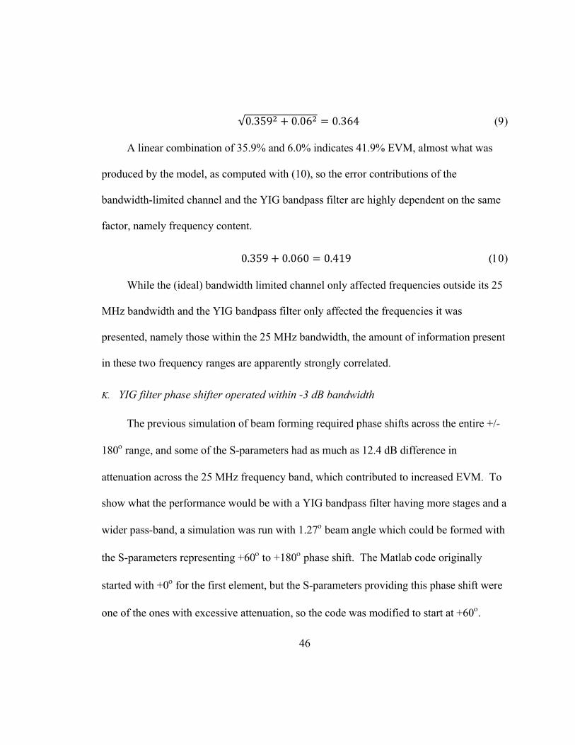
√0.359 0.06 0.364
A linear combination of 35.9% and 6.0% indicates 41.9% EVM, almost what was
produced by the model, as computed with (10), so the error contributions of the
bandwidth-limited channel and the YIG bandpass filter are highly dependent on the same
factor, namely frequency content.
0.359 0.060 0.419
While the (ideal) bandwidth limited channel only affected frequencies outside its 25
MHz bandwidth and the YIG bandpass filter only affected the frequencies it was
presented, namely those within the 25 MHz bandwidth, the amount of information present
in these two frequency ranges are apparently strongly correlated.
K. YIG filter phase shifter operated within -3 dB bandwidth
The previous simulation of beam forming required phase shifts across the entire +/-
180 range, and some of the S-parameters had as much as 12.4 dB difference in
attenuation across the 25 MHz frequency band, which contributed to increased EVM. To
show what the performance would be with a YIG bandpass filter having more stages and a
wider pass-band, a simulation was run with 1.27 beam angle which could be formed with
the S-parameters representing +60 to +180 phase shift. The Matlab code originally
started with +0 for the first element, but the S-parameters providing this phase shift were
one of the ones with excessive attenuation, so the code was modified to start at +60.

47
When re-run the EVM decreased to 4.4%. The reason the impact of the YIG phase shifter
on distortion was not greater when operated beyond the -3 dB point was that the
contribution was reduced; this is what caused the decreased gain when the radiation
pattern was calculated. Using a YIG filter with sufficient bandwidth would do more to
improve gain than EVM, as variations in gain across frequency were averaged out. It is
also interesting to note that the delta constellation error appears uniformly distributed
between I and Q independently (Fig. 23); there is not a correlation between I and Q error
as occurred with the earlier, more highly distorting channels.
Once again, the recovered constellation and I & Q data have significant distortion.
Figure 23. Recovered constellation and delta error YIG vs. baseline for small angle

48
L. Swept beam angle using YIG filter phase shifter
The particular amount of phase shift required at each antenna element varies with the
beam angle. In the case of a 30 beam angle and antenna elements separated by one
wavelength, only two phase shifts are used by all the antenna elements, e.g. just 0 or
+180. Because attenuation (and slope of attenuation vs. frequency) from the YIG filter
that was characterized was considerably greater than desired for some selected phase
shifts, both signal strength and EVM vary with beam angle. A simulation was run
sweeping beam angle from 0 to +90. The results are plotted in Fig. 24.
The EVM for 0 was higher at 12% due to the characteristics of the single S-
parameter which was used for all antenna elements. Most other beam angles averaged out
the non-ideal behavior of a number of S-parameters. When the code was modified so the
0 beam angle used only the center of the YIG bandpass filter, which had a +120 phase
shift, EVM for that beam angle was reduced to 2.7%. (A lumped-element bandpass filter
with zero dimensions, such as the ideal Butterworth filter described previously, exhibits no
phase shift at the center of the pass band. A physical implementation such as the YIG
bandpass filter has length through which the signal must propagate, introducing
frequency-dependent phase shift.)

49
Once again, the recovered constellation and I & Q data have significant distortion.
Figure 24. EVM variation as beam swept from 0 to +90 by YIG phase shifter

50
VIII. ISSUES IDENTIFIED IN PHASED ARRAY SYSTEMS
Phased array antenna systems are used as an alternative to dish antennas when it is
preferred to have no moving parts, often for reasons of cost, maintenance, or speed of
sweeping/hopping. There are important differences, however.
Even for a continuous tone, it is readily apparent that the radiation pattern has a
number of side lobes where signals from the antenna elements constructively interfere.
For transmitter applications this is simply lost power, but for receivers, if selectivity
between transmitting sources is to be based on spatial separation rather than frequency,
signals from other sources that happen to be located in the side lobes will also be received.
Modulated data is replicated over some number of cycles of the carrier frequency.
For instance, in the analysis provided here, each symbol was encoded as a single cycle at
12.5 MHz (modulated and filtered such that it occupied 25 MHz bandwidth), then mixed
up to 10 GHz. Accordingly, the symbol is transmitted as modulation on 800 cycles of the
carrier. While all energy directed by a dish antenna would arrive at (or from) a remote
antenna at the same time due to equal path length (except for group delay caused by
differences in propagation velocity through the intervening medium, the atmosphere), this
is not the case with phased array. Up to one cycle of phase shift might be accomplished
with signal delayed by the appropriate amount, but if for instance 540 is required for an
antenna element located 1.5 wavelengths further from the target than another, only 180 is
provided. This provides proper constructive interference of the carrier signal, but overlaps
one cycle of carrier signal carrying a given modulated symbol with a cycle of carrier

51
signal carrying the previous symbol. For the notional system using 800 cycles of carrier to
represent each symbol, this would only be one cycle of interference vs. 799 without such
corruption. However, for systems where the symbol rate is closer to carrier frequency, or
where the antenna array spans a greater number of wavelengths, the effect would be
greater. While the impact on EVM could be reduced by pre- or post-compensation
correcting the modulation level depending on adjacent bits, such an approach would not
reduce the impact on antenna gain. What would be required to fully address the issue is
phase shift spanning multiple 360 cycles. This could be accomplished in the RF domain
with additional stages of filter for YIG or Varactor based phase shifters or additional
lengths of coax/microstrip for delay-line phase shifters. Alternatively it could be
addressed in the digital domain for systems generating/recovering data from the
modulated signal on a per-element basis.
Because a frequency-domain mathematical approach was taken to combine wave-
fronts from antenna elements, the work presented here does not incorporate the effects of
overlapping modulated symbols described above. For analysis of a system where the
symbol rate is sufficiently close to carrier frequency for this effect to be significant, the
modulated bit stream could be shifted by a multiple of the carrier period prior to
converting it to the frequency domain.

52
IX. POTENTIAL PITFALLS OF CHARACTERZATION AND ANALYSIS APPROACH
The approach of measuring individual components and simulating overall system
performance is convenient, but leaves open the possibility for various mistakes. A
common error in SPICE simulation is to capture an output waveform from one circuit
(driving an anticipated load, or no load at all), then to apply that waveform as a voltage
source with zero impedance to the next stage. If the actual impedance of the next stage
input is different, the applied stimulus will be incorrect. The approach taken in RF and
microwave modeling, interconnecting various S-parameter blocks (or other
representations) is meant to avoid such problems by presenting appropriate complex
impedances. Another concern for characterization of the phase shifter is that
measurements by the Vector Network Analyzer (VNA) may represent an average of
multiple cycles. Averaging is useful to remove random errors or noise. However,
instantaneous phase shift for a single cycle is required, because in phased array
applications instantaneous waveforms from each antenna element combine to generate the
wavefront.
Besides implementing an actual phased array antenna system and performing an
over the air measurement, an alternative test would be to combine phase-shifted and non-
phase-shifted signals. This can be performed with a splitter, followed by the phase-shifter
for one channel and an attenuator for the other, and then a combiner. The attenuator
models a (fixed) phase shifter by simply providing a similar loss. The measured

53
combination of the two channels will match the calculated combination only if the random
variations in phase shift are not too significant.

54
X. ON IMPLEMENTING AN ACTUAL SYSTEM
For purposes of characterizing the EVM contribution of a YIG phase shifter, a
notional digital radio system was implemented in Matlab, modeling idealized components.
Several changes would ease implementation with actual hardware. Selecting a higher
frequency IF would reduce the errors introduced by variations in LO. Prior to recovering
the I and Q bitstream, the IF data sample could be analyzed to determine the precise IF
frequency it contained; this would correct for oscillator variation as well as Dopler shift.
Filtering and compensation would be performed to limit the channel bandwidth required
and reduce inter-symbol interference.

55
XI. CONCLUSION
The original hypothesis, that a YIG band-pass filter providing precise phase shift
would result in a higher gain phased array antenna system than one using discrete delay
lines, was found not to be true. With 45 increments in phase shift there is little reduction
in gain compared to ideal phase shifters.
The commercially available YIG filter selected for this work did not have sufficient
phase shift in the passband to carry a 25 MHz bandwidth signal while tuning for +/- 180
phase shift. It was likely built with two YIG spheres rather than four; this would be
consistent with the insertion loss it displayed. Despite the frequency-dependent
attenuation it exhibited under some operating conditions, the simulated contribution to
system EVM of around 6% that resulted suggests it would work in an actual system.
While the YIG phase shifter did not show improved beam forming compared to
discrete delay line shifters, it may still be useful for rapid beam sweeping. When a large
number of antenna elements is used for high gain, the beam angle will have to be changed
more frequently to track a rapidly moving target. If relays are used to switch delay lines,
the millisecond switching delay could result in reduced gain or having the beam off the
target. A continuously variable phase shifter such as YIG (or varactor for lower
frequencies) could still provide a benefit in that case.

56
APPENDIX A. MATLAB CODE
This section contains listings of all Matlab code used for processing and analysis of the data. It was executed under Matlab
version 7.7.0.471 (R2008b).
A. Radiation pattern
The function ‘plot_antenna_pattern_n_dipole’ is the top level routine used to generate a surface representing the radiation
pattern of a phased array.
function XX = plot_antenna_pattern_n_dipole
% EE299 Thesis - Test antenna_pattern routine
% Consider "n" dipoles, separated by pitch
% [x,y,z] = sph2cart(THETA,PHI,R)
% note 'PHI' is angle from X-Y plane
% i.e. straight up = 90 degrees, not 0 degrees as in Electromagnetics
% use [Matlab] PHI = 90 - [Electromagnetics] FI
disp('Antenna Elements')
57
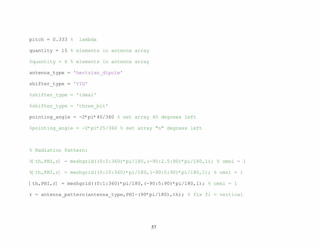
pitch = 0.333 % lambda
quantity = 15 % elements in antenna array
%quantity = 4 % elements in antenna array
antenna_type = 'hertzian_dipole'
shifter_type = 'YIG'
%shifter_type = 'ideal'
%shifter_type = 'three_bit'
pointing_angle = -2*pi*40/360 % set array 40 degrees left
%pointing_angle = -2*pi*25/360 % set array "n" degrees left
% Radiation Pattern:
%[th,PHI,r] = meshgrid((0:5:360)*pi/180,(-90:2.5:90)*pi/180,1); % omni = 1
%[th,PHI,r] = meshgrid((0:10:360)*pi/180,(-90:5:90)*pi/180,1); % omni = 1
[th,PHI,r] = meshgrid((0:1:360)*pi/180,(-90:5:90)*pi/180,1); % omni = 1
r = antenna_pattern(antenna_type,PHI-(90*pi/180),th); % fix fi = vertical
58
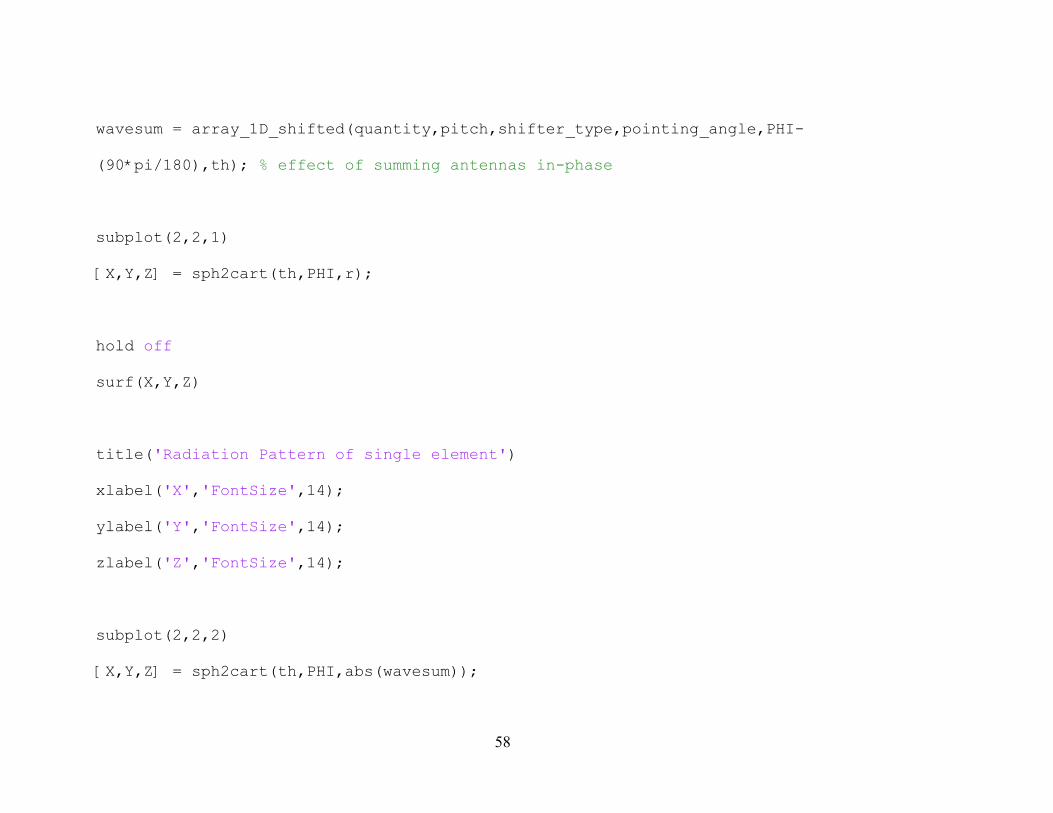
wavesum = array_1D_shifted(quantity,pitch,shifter_type,pointing_angle,PHI-
(90*pi/180),th); % effect of summing antennas in-phase
subplot(2,2,1)
[X,Y,Z] = sph2cart(th,PHI,r);
hold off
surf(X,Y,Z)
title('Radiation Pattern of single element')
xlabel('X','FontSize',14);
ylabel('Y','FontSize',14);
zlabel('Z','FontSize',14);
subplot(2,2,2)
[X,Y,Z] = sph2cart(th,PHI,abs(wavesum));

59
surf(X,Y,Z)
title('Constructive/Destructive Interference')
subplot(2,2,3)
[X,Y,Z] = sph2cart(th,PHI,abs(r.*wavesum));
surfc(X,Y,Z)
title(sprintf('Combined Radiation Pattern of all %d elements at pitch %0.1g
lambda',quantity,pitch))
subplot(2,2,4)
polar(th,abs(r.*wavesum));

60
B. Antenna pattern
The function ‘antenna_pattern’, given an input of angles (in this case representing 360 degrees around and 180 degrees up
and down) returns the radiation pattern of a single antenna element.
function X = antenna_pattern(antenna_type,theta,fi)
% EE299 Thesis - For an antenna (patch, dipole, etc) given angle,
% return gain in that direction
switch antenna_type
case 'hertzian_dipole',
% directivity of hertzian dipole is 1.5 or +1.76 dB
X = 1.5 * sin(theta).^2;
otherwise,
X = 0;
disp(antenna_type)
disp(': antenna type not modeled')
end
61
C. Constructive and destructive interference
The function ‘array_1D_shifted’, returns the pattern of constructive and destructive interference from elements of a phased
array. It is the radiation pattern that would occur if the antenna elements were spherical radiators (omni-directional).
function X = array_1D_shifted(quantity,pitch,shifter_type,pointing_angle,theta,fi)
% EE299 Thesis - For an antenna array given angle,
% Calls routine to look up shift and attenuation,
% sum effect of each antenna element
% return complex number representing constructive/destructive
% interference in given direction.
%(pattern of each antenna handled in a separate routine)
% theta ignored because it is vertical angle, and array assumed horizontal
if quantity < 1
disp('quantity of antenna elements must be a positive integer')
% end
62
elseif rem(quantity,1) == 0
% everything OK
e_vector = 0;
shift_and_magnitude = [0.0,0.0]; %[fi_prime, attenuation]
shifts_and_magnitudes = zeros(quantity,2);
%shifts_and_magnitudes
for index = 0:1:quantity-1
shift_and_magnitude = phase_shift(shifter_type,pointing_angle,pitch,index);
e_vector = e_vector + shift_and_magnitude(2) *
exp(1j*(index*pitch*sin(fi)*2*pi-shift_and_magnitude(1))); % antenna element 'index'
shifts_and_magnitudes(index+1,:) = shift_and_magnitude;
% build array of shift at each antena element
end

63
X = e_vector;
shifts_and_magnitudes % display array
subplot(3,2,5)
plot(shifts_and_magnitudes)
else
disp('Only integer quantity of antenna elements supported')
end
D. Phase shifter
The function ‘phase_shift’ computes the distance from a given antenna element to the wavefront in lambda and
returns magnitude and phase for selected type of shifter.
function X = phase_shift(shifter_type,pointing_angle,pitch,index)
% EE299 Thesis -
% shift_and_magnitude = phase_shift(shifter_type,pointing,pitch,index);

64
switch shifter_type
case 'ideal',
shift = sin(pointing_angle)* pitch * index * 2*pi
X = [shift,1.0];
case 'three_bit', % 45 degree increments of coax
shift = pi/4*round(sin(pointing_angle)* pitch * index * 2*pi/(pi/4));
X = [shift,1.0];
case 'YIG',
idealshift = sin(pointing_angle)* pitch * index * 2*pi
degrees = 360*idealshift/(2*pi)
% range of possible inputs: beyond -180 degrees to +180 degrees
index = round(rem(degrees,360)/10 + 18 - 0.5)+1
% snap to nearest 10 degree increment in allowed range
Sparm_arraysize = 36; % number of separate SParms

65
index = mod(index-1,Sparm_arraysize-1)+1;
% wrap around beyond 360 degrees, but 1..36, not 0..35
MAG_51 = load('YIG_data\MAG.txt'); % Load SParm data
PHASE_51 = load('YIG_data\PHASE.txt');
freq_10G_index = 26; % position in SParm for nominal frequency
YIG_loss = -2.6; % dB loss at center of pass band
gain = 10^((MAG_51(freq_10G_index,index)-YIG_loss)/20)
% convert dB to magnitude
%In previous line, gain of -2.6 dB was normalized to 0 dB.
%e.g. amplifier restores signal
shift = PHASE_51(freq_10G_index,index)/360 * 2*pi % return in radians
X = [shift,gain];
otherwise,
X = 0;
disp(shifter_type)

66
disp(': shifter type not modeled')
end
shift/(2*pi) * 360 % display degrees shift
E. Digital radio model and EVM calculation
The function ‘FFT_test_filtered’ is the top level routine used to simulate a QAM-16 digital radio and determine EVM
when passing through a channel, for instance a phased array antenna system. When called with it produces plots of modulated
IF data, constellations, errors seen at demodulation, and spectral content. It also returns EVM computed as the RSS of errors
from each symbol recovered.
function X = FFT_test_filtered(beam_angle_degrees)
% EE299 Thesis - I-Q Modulate bit stream and transmit through channel
% filtered - Butterworth, YIG phase shifter (or other) filter transfer function
% recover I-Q symbols and compute EVM
% Also recover transmitted signal which is bandwidth limited but not
% filtered by the channel to determine increase in EVM due to phase shifter
67
% set up symbol rate
symbol_rate = 12.5e6 % 12.5 MHz symbol rate
points = 20; %
per symbol 20 for good resolution to represent one cycle sine wave
Fs = symbol_rate * points; % sample rate 250 MHz
LO = 10e9 - symbol_rate;
%beam_angle = pi/6 % 30 degrees % phase shift only two values required
beam_angle = beam_angle_degrees/360 * 2* pi
%beam_angle = 40/360 * 2* pi % 40 degrees
numelements = 15
%numelements = 3
array_pitch = 1 % lambda or wavelengths
68
%shifter_type = 'ideal'
%shifter_type = 'three_bit'
%shifter_type = 'butterworth'
shifter_type = 'YIG'
%shifter_type = 'none'
plot_selection = 'debug'
plot_selection = 'transmitted'
plot_selection = 'modulated'
plot_selection = 'recovered'
% 16-QAM: 4 bits encoded in sixteen spots
bits_per_symbol = 4; % for hexidecimal
bits_per_half_symbol = bits_per_symbol/2;
value_per_half_symbol = 2^bits_per_half_symbol;

69
%bitstream_in = [0 1 2 3 4 5 6 7 8 9 10 11 12 13 14 15]' % for hexidecimal
bitstream_in = [0 15 4 11 8 7 12 3 13 2 14 1 10 5 6 9]' % bolt torqing pattern
%bitstream_in = [5 6 10 9 4 0 1 2 3 7 11 15 14 13 12 8]' % spiral out for
hexidecimal
symbols = 16;
% Split each symbol in half (low/high)
bithigh_in = floor(bitstream_in ./ value_per_half_symbol);
bitlow_in = mod(bitstream_in,value_per_half_symbol);
bithigh_centered = bithigh_in - (value_per_half_symbol/2 - 0.5);
bitlow_centered = bitlow_in - (value_per_half_symbol/2 - 0.5);
subplot(5,3,1)
plot(bitlow_centered,bithigh_centered,'o--')
title('Traversing the Constellation')

70
xlabel('I');
ylabel('Q');
subplot(5,3,4)
stem(bitlow_centered)
title('I')
ylabel('I');
subplot(5,3,7)
stem(bithigh_centered)
title('Q')
ylabel('Q');
% generate cos wave for I
symbol_freq = 12.5; % MHz
sample_freq = symbol_freq * points

71
% 80 ns/symbol, 20 points each, 4 ns per sample
t = 0:1/sample_freq:(points-1)/sample_freq; % time domain timebase
coswave = cos(2*pi*t*sample_freq/points + pi/4)';
hold off
subplot(5,3,2)
plot(t,coswave,'r')
sinwave = -sin(2*pi*t*sample_freq/points + pi/4)';
hold on
subplot(5,3,2)
plot(t,sinwave,'b')
title('cos & -sin for I & Q modulation')
hold off
% Piece-wise linear I & Q

72
I = [];
Q = [];
tt = [];
for index = 0:1:symbols-1
I = [I; bitlow_centered(index+1) * coswave];
Q = [Q; bithigh_centered(index+1) * sinwave];
tt = [t, tt+points/sample_freq];
end
subplot(5,3,5)
plot(tt,I')
title('cosine modulation of I')
subplot(5,3,8)
plot(tt,Q)
title('sine modulation of Q')

73
IQ_signal = I + Q;
subplot(5,3,3)
plot(tt,IQ_signal)
title('IQ modulation of bit stream')
% Done with time domain. Convert to frequency domain
IQ_signal_f = fft(IQ_signal,512); % 512 is a power of 2 > 320
% Implement a brick-wall digital filter to eliminate IF frequency
% components > 2x IF. Otherwise LO + IF and LO - IF overlap.
pass = 52; % pass first 50 frequency points un-altered = 25 MHz
halfpoints = length(IQ_signal_f)/2;
brick_wall = [ones(1,pass),zeros(1,halfpoints-pass), zeros(1,halfpoints-
pass),ones(1,pass)]'; % double-sided

74
% Filter IF signal
IQ_signal_f_transmitted = (IQ_signal_f .* brick_wall);
% Create array of frequencies for graphing/filtering purposes
NFFT = 2^nextpow2(length(IQ_signal));
% Next power of 2 from length of y e.g. 512 is a power of 2 > 320
f = Fs/2*linspace(0,1,NFFT/2+1); % out of 512 points, 257 = 512/2 + 1
%save 'debug_f.txt' f -ASCII % save in file for debug purposes
switch shifter_type
case 'butterworth',
onesided_filter =
beamform_bandbutter_8th(f+LO,beam_angle,numelements,array_pitch);

75
case 'YIG',
onesided_filter = beamform_YIG(f+LO,beam_angle,numelements,array_pitch);
otherwise,
disp(shifter_type)
disp(': shifter type not modeled; replace with ideal but BW limited
channel')
% turn off channel degredation - revert to baseline
onesided_filter = ones(1,NFFT/2+1);
end
doublesided_filter = [onesided_filter,
conj(fliplr(onesided_filter(2:length(onesided_filter)-1)))]';
% actual orientation of frequency points in array
doublesided_filter(NFFT/2+1) = 0; % even number of bits, first is DC. Kill the
one positive freq without corresponding negative freq

76
subplot(5,3,13)
degrade_phase = doublesided_filter; % Apply selected filter as phase shifter
degrade = degrade_phase; % a channel response by any other name
semilogy(abs(degrade)) % plot magnitude so complex isn't plotted real vs.
imaginary
title('Channel response')
IQ_signal_f_received = (IQ_signal_f_transmitted .* degrade); % linear rolloff
% The received signal has been shifted in time/phase
% shift back to synchronize for recovery of data
phase_correct = correct_delay(degrade_phase);
IQ_signal_f_corrected = IQ_signal_f_received .* phase_correct;
% Done with frequency domain. Convert back to time domain

77
IQ_signal_recovered = ifft(IQ_signal_f_corrected);
% As a baseline for comparison, also convert original signal without
degredation
IQ_signal_baseline = ifft(IQ_signal_f_transmitted);
% Now recover each symbol
% First, extract the timeslice with an IQ (QAM-16) encoding
bitlow_recovered = [];
bithigh_recovered = [];
bitlow_baseline = [];
bithigh_baseline = [];
for index = 0:1:symbols-1
IQ_timeslice = IQ_signal_recovered(index*points +1:index*points +points);

78
bitlow_recovered = [bitlow_recovered; 2*mean(IQ_timeslice .* coswave)]; %
"mean" serves to integrate over period
bithigh_recovered = [bithigh_recovered; 2*mean(IQ_timeslice .* sinwave)];
IQ_baseline = IQ_signal_baseline(index*points +1:index*points +points);
bitlow_baseline = [bitlow_baseline; 2*mean(IQ_baseline .* coswave)];
% "mean" serves to integrate over period
bithigh_baseline = [bithigh_baseline; 2*mean(IQ_baseline .* sinwave)];
end
subplot(5,3,6)
stem(real(bitlow_recovered))
title('I recovered')
ylabel('I recovered');
subplot(5,3,9)

79
stem(real(bithigh_recovered))
title('Q recovered')
ylabel('Q recovered');
bitlow_centered
bitlow_recovered
subplot(5,3,10)
plot(real(bitlow_recovered),real(bithigh_recovered),'o--')
title('Recovered Constellation')
xlabel('I');
ylabel('Q');
% find error between original and recovered 'I' and 'Q'
bitlow_error = bitlow_recovered - bitlow_centered;
bithigh_error = bithigh_recovered - bithigh_centered;

80
% find error between baseline and recovered 'I' and 'Q'
bitlow_delta_error = bitlow_recovered - bitlow_baseline;
bithigh_delta_error = bithigh_recovered - bithigh_baseline;
subplot(5,3,11)
plot(real(bitlow_error),real(bithigh_error),'o--')
title('Constellation Error')
xlabel('I error');
ylabel('Q error');
% Compute RMS error
RMS_error = (mean([bitlow_error.^2; bithigh_error.^2]))^0.5
EVM_percent = RMS_error/0.5 * 100
RMS_delta_error = (mean([bitlow_delta_error.^2; bithigh_delta_error.^2]))^0.5

81
EVM_delta_percent = RMS_delta_error/0.5 * 100
X = EVM_delta_percent; % Give as return from this function
% study behavior of fft on coswave
coswave_f = fft(coswave); % frequency domain of coswave
sinwave_f = fft(sinwave); % frequency domain of sinwave
% Construct a frequency axis
fftpoints = 1:1:512;
subplot(5,3,12)
hold off
plot(fftpoints,abs(IQ_signal_f),'r')
hold on
plot(fftpoints,abs(IQ_signal_f_transmitted),'b')

82
hold off
title('IQ signal f frequency domain')
xlabel('frequency (Mhz)');
ylabel('|signal|');
coswave_recovered = ifft(coswave_f);
sinwave_recovered = ifft(sinwave_f);
hold off
subplot(5,3,14)
plot(t,coswave_recovered,'r')
hold on
subplot(5,3,14)
plot(t,sinwave_recovered,'b')
title('recovered cos & -sin for I & Q modulation')

83
hold off
% overwrite with different plot
subplot(5,3,14)
plot(real(bitlow_delta_error),real(bithigh_delta_error),'o--')
title('delta Constellation Error')
xlabel('I error');
ylabel('Q error');
% plot error
hold off
subplot(5,3,15)
plot(t,coswave_recovered - coswave,'r')
hold on
subplot(5,3,15)

84
plot(t,sinwave_recovered - sinwave,'b')
title('error in recovered cos & -sin')
hold off
% overwrite with different plot
hold off
plot(fftpoints,angle(degrade_phase),'b')
hold on
plot(fftpoints,angle(phase_correct),'r')
hold off
title('filter phase')
xlabel('frequency (Mhz)');
ylabel('phase of filter');
F. Idealized Butterworth beam former
The function ‘beamform_bandbutter_8th’ returns the S-parameters (normalized to 1.0 magnitude at center frequency) for a
phased array antenna system, with an idealized Butterworth filter serving as phase shifter.

85
function X = beamform_bandbutter_8th(f,beam_angle,numelements,pitch)
% model beamforming using 8th order bandpass filter as phase-shifter
% called with a set of frequency points and beam angle, returns S21 parameters
% Works by summing delayed results from phaseshift_bandbutter_8th
formedbeam = zeros(1,length(f));
for element = 1:1:numelements
phase_angle = rem((sin(beam_angle) * (element-1) * pitch * 2*pi)+pi, 2*pi)-
pi
delay = exp(-1j.*phase_angle*f./f(26));
angle(delay(26))
abs(delay(26))
phaseshifted_wavefront = phaseshift_bandbutter_8th(f,phase_angle);
angle(phaseshifted_wavefront(26))
delayed_wavefront = -delay .* phaseshifted_wavefront;
86
angle(delayed_wavefront(26))
formedbeam = formedbeam + delayed_wavefront;
end
net_multiple = abs(formedbeam(26)) % errors in picking phase - re-scale output
amplitude
formedbeam = formedbeam ./ net_multiple;
X = formedbeam; % return S21 parameter
G. Idealized Butterworth phase shifter
The function ‘phaseshift_bandbutter_8th’ estimates the center frequency a Butterworth band-pass filter should be tuned to
in order to produce the desired phase shift and returns S-parameters.
function X = phaseshift_bandbutter_8th(f,angle)
% model beamforming using 8th order bandpass filter as phase-shifter
% called with a set of frequency points and beam angle, returns S21 parameters

87
% with settings wl = 1.5*w; wh = 0.667*w;
% +209 degrees at 4.3e10 rad/sec
% 0 degrees at 6.28e10 rad/sec
% -200 degrees at 9.06e10 rad/sec
% find two slopes, one for positive phase shift, the other negative phase shift
plus209freq = 4.3e10/(2*pi);
plus0freq = 6.28e10/(2*pi);
minus200freq = 9.06e10/(2*pi);
plus_degrees_per_hz = 209 /(plus209freq - plus0freq);
plus_radians_per_hz = 2*pi*plus_degrees_per_hz/360;
plus_hz_per_radian = 1/plus_radians_per_hz;
minus_degrees_per_hz = (209 - (-200))/(plus209freq - minus200freq);
88
minus_radians_per_hz = 2*pi*minus_degrees_per_hz/360;
minus_hz_per_radian = 1/minus_radians_per_hz;
fnom = 10e9; % 10 GHz nominal frequency for no phase shift
angle;
if angle >= 0
offnom = fnom + angle * plus_hz_per_radian;
else
offnom = fnom + angle * minus_hz_per_radian;
end
w = 2*pi*offnom; % radians
% following values for broad passband
wl = 1.5*w; % cutoff by lowpass filter; high frequency cutoff of bandpass
wh = 0.667*w; % cutoff by highpass filter; low frequency cutoff of bandpass

89
glow = tf([1],[1/wl^8 5.1258/wl^7 13.13695771/wl^6 21.84596388/wl^5 25.6881355/wl^4
21.84596388/wl^3 13.13695771/wl^2 5.1258/wl 1]);
ghigh = tf([1/wh^8 0 0 0 0 0 0 0 0],[1/wh^8 5.1258/wh^7 13.13695771/wh^6
21.84596388/wh^5 25.6881355/wh^4 21.84596388/wh^3 13.13695771/wh^2 5.1258/wh 1]);
g = glow * ghigh;
%bode(g)
[MAG,PHASE] = bode(g,f*2*pi);
SPARM = MAG(:,:).*cos(2*pi/360*PHASE(:,:)) + 1i *
MAG(:,:).*sin(2*pi/360*PHASE(:,:));
X = SPARM; % return S21 parameter
H. Recovery synchronization
The function ‘correct_delay’ determines the phase shift introduced in the center of the IF frequency by the S-parameters
representing the sum of the contribution of all antenna elements (each of which is at a different distance from the target). In an

90
actual system this would be performed by adjusting a phase-locked loop or by analyzing the sampled IF waveform, but for
purposes of this model it is simply determined from the calculated channel response. This routine performs a second function as
well. For a phased array antenna the function which is actually desired from a phase shifter is to delay the signal to each
antenna element, irrespective of frequency, such that all reach the target destination at the same time. The phase shifter provides
the necessary relative shift between antenna elements to achieve constructive interference. However, by heavily filtering the
signals, the analog phase shifter introduces a frequency-dependent phase shift is introduced into the signal that is delivered to
the destination (or received.) This can be compensated for in the digital realm by pre-compensating transmitted signals or post-
compensating received signals based on characterized behavior. The function ‘correct_delay’ performs this with a simple linear
predicted response, the slope of the phase shift between the lowest frequency component in the signal and the center of the IF
frequency. The phase error which remains is due to non-linearity of the YIG phase shifter. While this code could have been
written with a calibration constant for the slope, it was instead made adaptive so as to work with any selected phase shifter (e.g.
the higher order ideal Butterworth filter.)
function X = correct_delay(filter_response)
% EE299 Thesis - given filter_response (a phase shifter)
% create an inverse phase filter to correct phase response at IF
% Presumption is the delay needs to be corrected. But, rather

91
% than introducing the time component into a frequency domain model,
% each frequency is just phase shifted. For signals which
% undergo more than 360 degrees shift this is not correct; antenna
% elements more than one IF cycle from the wavefront will carry
% modulated data from a different symbol
NFFT = length(filter_response);
IF_index = 26; % The IF frequency is represented by element 26 in array
% unwind phase shift from filter
shift_IF = angle(filter_response(IF_index))
% phase shift at location of 1/2 IF
shift_min_f = angle(filter_response(2))
% phase shift at lowest frequency component
if (shift_IF < 0) && (shift_min_f > 0)
shift_IF = shift_IF + 2*pi;

92
% wrapped around because > +1 pi; represent as +1.x pi
end
shift_slope = (shift_IF-shift_min_f)/(IF_index-1);
points_slope = 2:1:NFFT/2;
linear_slope = exp(- 1i .* (shift_IF + (points_slope - IF_index) .*
(shift_slope)))';
linear_correct = [1; linear_slope];
max_f_point = NFFT/2; % Half of points represent positive frequencies, the
other half negative frequencies
phase_correct = zeros(1,NFFT);
phase_correct(1:max_f_point) = linear_correct;
% linear slope for positive frequencies
phase_correct(NFFT-max_f_point+2:NFFT) =
conj(flipud((linear_correct(2:max_f_point))));
93
% reverse slope for negative frequencies
phase_correct = phase_correct';
X = phase_correct;
I. YIG beam former
The function ‘beamform_YIG’ returns the S-parameters (normalized to 1.0 magnitude at center frequency) for a phased
array antenna system using measured YIG bandpass filter S-paramters.
function X = beamform_YIG(f,beam_angle,numelements,pitch)
% model beamforming using measured YIG SParms
% called with a set of frequency points and beam angle, returns S21 parameters
% representing channel response in direction of beam
% Instead of starting at zero degrees, start at +60 degrees so very small
% angles can be obtained with the +60 to +180 angles for which
% the measured YIG filter was within its -3dB passband
first_element_angle = 60; % degrees
94
rad_start = first_element_angle/360 * 2 * pi; %radians
% Works by summing delayed results from phaseshift_YIG
formedbeam = zeros(1,length(f));
for element = 1:1:numelements
phase_angle = rem((sin(beam_angle) * (element-1) * pitch)+pi + rad_start,
2*pi)-pi
delay = exp(-1j.*phase_angle*f./f(26));
% Compute phase shift from delay between antenna element and wavefront
abs_delay = abs(delay(26)) % debug
degrees_angle_delay = angle(delay(26)) *360/(2*pi) % debug
phaseshifted_wavefront = phaseshift_YIG(f,phase_angle);
abs_phaseshift = abs(phaseshifted_wavefront(26)) % debug

95
degrees_angle_phaseshift = angle(phaseshifted_wavefront(26)) *360/(2*pi) %
debug
delayed_wavefront = -delay .* phaseshifted_wavefront;
% Propagation delay shifts phase of each frequency
abs_delayed_wavefront = abs(delayed_wavefront(26)) % debug
degrees_angle_delayed_wavefront = angle(delayed_wavefront(26)) *360/(2*pi) %
debug
formedbeam = formedbeam + delayed_wavefront;
end
% Automatic Gain Control should be processed in receiver/de-modulator
% But to keep it simple, channel gain is normalized to 1.0 at center
% frequency:
net_multiple = abs(formedbeam(26)) % re-scale output amplitude for 1.0 output

96
formedbeam = formedbeam ./ net_multiple;
X = formedbeam; % return S21 parameter
J. YIG phase shifter
The function ‘phaseshift_YIG’ looks up an S-parameter file with phase shift closest to the desired amount. The files
provide 10 degree increments, so the result is within +/- 5 degrees.
function X = phaseshift_YIG(f,angle)
% beamforming using measured SParms from YIG filter as phase-shifter
% called with a set of frequency points and beam angle, returns S21 parameters
fnom = 10e9; % 10 GHz nominal frequency for no phase shift
angle;
degrees = 360*angle/(2*pi) % range of possible inputs: -180 degrees to +180 degrees
index = round(rem(degrees,360)/10 + 18 - 0.5)+1 % snap to nearest 10 degree
increment

97
% load SParms from file
MAG_51 = load('YIG_data\MAG.txt');
PHASE_51 = load('YIG_data\PHASE.txt');
zip = -1e+5; % pad with values near zero outside 25MHz bandwidth
dB_MAG = [zip*ones(1,1),MAG_51(:,index)',zip*ones(1,257-51-1)];
% out of 512 points, 257 = 512/2 + 1
PHASE = [zeros(1,1),PHASE_51(:,index)',zeros(1,257-51-1)];
% out of 512 points, 257 = 512/2 + 1
% measured S-parm file was logarithmic; change to linear before
% creating complex values
MAG = 10.^(dB_MAG./20); % MAGDB = 20*log10(MAG);

98
SPARM = MAG(:,:).*cos(2*pi/360*PHASE(:,:)) + 1i *
MAG(:,:).*sin(2*pi/360*PHASE(:,:));
X = SPARM; % return S21 parameter
K. Swept beam angle
The function ‘EVM_test’ invokes FFT_test_filtered() with beam angles from 0 to +85 and produces a graph of EVM vs.
beam angle.
function X = EVM_test
% Sweep beam angle, report EVM
angle = []
delta_EVM = []
for angle_degrees = 0:5:85;
angle = [angle,angle_degrees];
delta_EVM = [delta_EVM,FFT_test_filtered(angle_degrees)]

99
end
subplot(5,3,13)
plot(angle,abs(delta_EVM))
title('delta EVM due to YIG phase shifter')
xlabel('beam angle (degrees)');
ylabel('delta EVM');
L. Read S-parameter files and store in array
The function ‘load_test’ reads 36 S-parameter files (that have had the header information removed for easier parsing) and
extracts the frequency, S21 magnitude, and S21 phase information. It stores these in three files for use by the other programs
and plots a family of curves for magnitude and phase.
function X = load_test
% Loading s-paramter files, save arrays of frequency, S21_mag, S21_phase

100
% case for plotting. plots 4 & 6 final
plot_selection = 'debug'
plot_selection = 'final'
% format:
% !S2P File: Measurements: S11, S21, S12, S22:
% # Hz S dB R 50
% freq S11_mag S11_degrees S21_mag S21_degrees S12_mag S12_degrees S22_mag
S22_degrees
datafiles =
['YIG_data\yigm_180.txt';'YIG_data\yigm_170.txt';'YIG_data\yigm_160.txt'];
datafiles =
[datafiles;'YIG_data\yigm_150.txt';'YIG_data\yigm_140.txt';'YIG_data\yigm_130.txt'];
datafiles =
[datafiles;'YIG_data\yigm_120.txt';'YIG_data\yigm_110.txt';'YIG_data\yigm_100.txt'];

101
datafiles = [datafiles;'YIG_data\yigm_90.txt ';'YIG_data\yigm_80.txt
';'YIG_data\yigm_70.txt '];
datafiles = [datafiles;'YIG_data\yigm_60.txt ';'YIG_data\yigm_50.txt
';'YIG_data\yigm_40.txt '];
datafiles = [datafiles;'YIG_data\yigm_30.txt ';'YIG_data\yigm_20.txt
';'YIG_data\yigm_10.txt '];
datafiles = [datafiles;'YIG_data\yigp_0.txt ';'YIG_data\yigp_10.txt
';'YIG_data\yigp_20.txt '];
datafiles = [datafiles;'YIG_data\yigp_30.txt ';'YIG_data\yigp_40.txt
';'YIG_data\yigp_50.txt '];
datafiles = [datafiles;'YIG_data\yigp_60.txt ';'YIG_data\yigp_70.txt
';'YIG_data\yigp_80.txt '];
datafiles = [datafiles;'YIG_data\yigp_90.txt
';'YIG_data\yigp_100.txt';'YIG_data\yigp_110.txt'];
datafiles =
[datafiles;'YIG_data\yigp_120.txt';'YIG_data\yigp_130.txt';'YIG_data\yigp_140.txt'];

102
datafiles =
[datafiles;'YIG_data\yigp_150.txt';'YIG_data\yigp_160.txt';'YIG_data\yigp_170.txt'];
datafiles(10,:)
fpoints = 51
fpoint_10G = 26;
num_sparms = 36
hold on
MAG = zeros(fpoints, num_sparms);
PHASE = zeros(fpoints, num_sparms);
for fileindex = 1:1:num_sparms;
yig_sparm = load(datafiles(fileindex,:));
f = yig_sparm(:,1);

103
MAG(:,fileindex) = yig_sparm(:,4);
PHASE(:,fileindex) = yig_sparm(:,5);
switch lower(plot_selection)
case 'debug'
subplot(3,2,1)
case 'final'
subplot(2,1,1) % will be overwritten
otherwise
subplot(3,2,1)
end
hold on
plot(f,MAG(:,fileindex))
title('Gain: Good except for some ripple')

104
switch lower(plot_selection)
case 'debug'
subplot(3,2,3)
case 'final'
subplot(2,1,1) % will be overwritten
otherwise
subplot(3,2,3)
end
hold on
plot(f,PHASE(:,fileindex))
title('Phase: Good except for slight ripple')
end

105
freq_plotted = f(fpoint_10G)
switch lower(plot_selection)
case 'debug'
subplot(3,2,5)
case 'final'
subplot(2,1,1) % will be overwritten
otherwise
subplot(3,2,5)
end
plot(MAG(fpoint_10G,:))
title('Response at 10 GHz as a function of selected phase shift')
MAG(:,fpoint_10G)
max(MAG)'

106
picked_index = 9 % an SParm with good representative flatness
picked_phase = PHASE(fpoint_10G,picked_index)
% What nominal 10GHz phase for that SParm
switch lower(plot_selection)
case 'debug'
subplot(3,2,2)
case 'final'
subplot(2,1,1) % will be overwritten
otherwise
subplot(3,2,2)
end
hold off
plot(f,MAG(:,picked_index))
title('Pick a Gain, any gain (e.g. index 9, -100 degrees)')
107
switch lower(plot_selection)
case 'debug'
subplot(3,2,4)
case 'final'
subplot(2,1,2) % will be overwritten
otherwise
subplot(3,2,4)
end
hold off
plot(f,PHASE(:,picked_index))
title('Phase of a Gain, any gain')
save 'YIG_data\MAG.txt' MAG -ASCII
save 'YIG_data\PHASE.txt' PHASE -ASCII
save 'YIG_data\f.txt' f -ASCII

108
switch lower(plot_selection)
case 'debug'
subplot(3,2,6)
case 'final'
subplot(2,1,2)
otherwise
subplot(3,2,6)
end
hold off
plot(f,PHASE(:,:))
title('Phase: Good except for slight ripple')
xlabel('frequency (Hz)');
ylabel('phase (degrees)');
% overwrite earlier plot:

109
switch lower(plot_selection)
case 'debug'
subplot(3,2,4)
case 'final'
subplot(2,1,1)
otherwise
subplot(3,2,4)
end
plot(f,MAG(:,:))
title('Gain: Good except for some ripple')
xlabel('frequency (Hz)');
ylabel('gain (dB)');

110
M. Read and plot filter S-parameter across entire passband
The function ‘load_bandpass’ reads 5 S-parameter files (that have had the header information removed for easier parsing)
and plots the data across a 200 MHz wide frequency range, showing the YIG filter’s 50 MHz -3 dB bandwidth centered about
the 10 GHz carrier frequency, then shifted up and down to provide +/- 180 phase shift relative to the centered one.
function X = load_bandpass
% Loading s-paramter files showing bandpass, 200 MHz bw around 10 GHz
% save arrays of frequency, S21_mag, S21_phase
% case for plotting. 4 & 6 final
plot_selection = 'debug'
plot_selection = 'final'
% Input format:
% !S2P File: Measurements: S11, S21, S12, S22:
% # Hz S dB R 50
111
% freq S11_mag S11_degrees S21_mag S21_degrees S12_mag S12_degrees S22_mag
S22_degrees
%filename strings padded with spaces to be same length
datafiles = ['YIG_data\yig_10g_left.txt ';'YIG_data\yig_10g_left_center.txt
';'YIG_data\yig_10g_center.txt '];
datafiles =
[datafiles;'YIG_data\yig_10g_right_center.txt';'YIG_data\yig_10g_right.txt '];
datafiles(3,:)
fpoints = 51
fpoint_10G = 26;
num_sparms = 5
hold on
MAG = zeros(fpoints, num_sparms);

112
PHASE = zeros(fpoints, num_sparms);
for fileindex = 1:1:num_sparms;
yig_sparm = load(datafiles(fileindex,:));
f = yig_sparm(:,1);
MAG(:,fileindex) = yig_sparm(:,4);
PHASE(:,fileindex) = yig_sparm(:,5);
switch lower(plot_selection)
case 'debug'
subplot(3,2,1)
case 'final'
subplot(2,1,1) % will be overwritten
otherwise

113
subplot(3,2,1)
end
hold on
plot(f,MAG(:,fileindex))
title('Gain: Good except for some ripple')
switch lower(plot_selection)
case 'debug'
subplot(3,2,3)
case 'final'
subplot(2,1,1) % will be overwritten
otherwise
subplot(3,2,3)
end
hold on

114
plot(f,PHASE(:,fileindex))
title('Phase: Good except for slight ripple')
end
freq_plotted = f(fpoint_10G)
switch lower(plot_selection)
case 'debug'
subplot(3,2,5)
case 'final'
subplot(2,1,1) % will be overwritten
otherwise
subplot(3,2,5)
end
plot(MAG(fpoint_10G,:))

115
title('Response at 10 GHz as a function of selected phase shift')
MAG(fpoint_10G,:)
max(MAG)'
picked_index = 3 % an SParm with good representative flatness
picked_phase = PHASE(fpoint_10G,picked_index)
% What nominal 10GHz phase for that SParm
switch lower(plot_selection)
case 'debug'
subplot(3,2,2)
case 'final'
subplot(2,1,1) % will be overwritten
otherwise
subplot(3,2,2)

116
end
hold off
plot(f,MAG(:,picked_index))
title('Pick a Gain, any gain (e.g. index 9, -100 degrees)')
switch lower(plot_selection)
case 'debug'
subplot(3,2,4)
case 'final'
subplot(2,1,2) % will be overwritten
otherwise
subplot(3,2,4)
end
hold off
plot(f,PHASE(:,picked_index))

117
title('Phase of a Gain, any gain')
save 'YIG_data\bandpass_MAG.txt' MAG -ASCII
save 'YIG_data\bandpass_PHASE.txt' PHASE -ASCII
save 'YIG_data\bandpass_f.txt' f -ASCII
switch lower(plot_selection)
case 'debug'
subplot(3,2,6)
case 'final'
subplot(2,1,2)
otherwise
subplot(3,2,6)
end
hold off

118
plot(f,PHASE(:,:))
title('Phase: Good except for slight ripple')
xlabel('frequency (Hz)');
ylabel('phase (degrees)');
% overwrite earlier plot:
switch lower(plot_selection)
case 'debug'
subplot(3,2,4)
case 'final'
subplot(2,1,1)
otherwise
subplot(3,2,4)
end
plot(f,MAG(:,:))
title('Gain: Good except for some ripple')

119
xlabel('frequency (Hz)');
ylabel('gain (dB)');
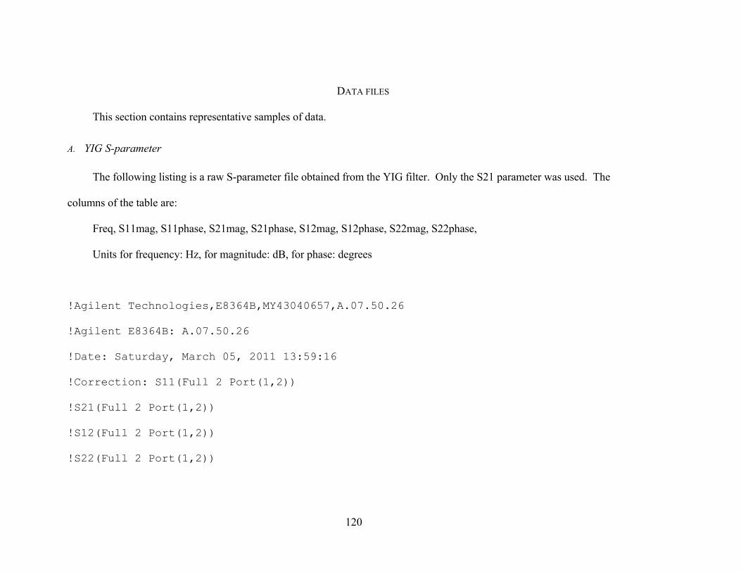
120
APPENDIX B. DATA FILES
This section contains representative samples of data.
A. YIG S-parameter
The following listing is a raw S-parameter file obtained from the YIG filter. Only the S21 parameter was used. The
columns of the table are:
Freq, S11mag, S11phase, S21mag, S21phase, S12mag, S12phase, S22mag, S22phase,
Units for frequency: Hz, for magnitude: dB, for phase: degrees
!Agilent Technologies,E8364B,MY43040657,A.07.50.26
!Agilent E8364B: A.07.50.26
!Date: Saturday, March 05, 2011 13:59:16
!Correction: S11(Full 2 Port(1,2))
!S21(Full 2 Port(1,2))
!S12(Full 2 Port(1,2))
!S22(Full 2 Port(1,2))

121
!S2P File: Measurements: S11, S21, S12, S22:
# Hz S dB R 50
9987790000 -2.137880e+001 1.084778e+002 -3.282870e+000 -4.311288e+001 -2.763350e+000
1.564315e+002 -1.843445e+001 1.686666e+002
9988278200 -2.107807e+001 1.085379e+002 -3.224191e+000 -4.595632e+001 -2.754102e+000
1.540602e+002 -1.796189e+001 1.709051e+002
9988766400 -2.083906e+001 1.085832e+002 -3.185504e+000 -4.863684e+001 -2.750721e+000
1.517571e+002 -1.748332e+001 1.719006e+002
9989254600 -2.069933e+001 1.087286e+002 -3.162029e+000 -5.113791e+001 -2.754327e+000
1.495369e+002 -1.700962e+001 1.720140e+002
9989742800 -2.053877e+001 1.089825e+002 -3.137861e+000 -5.349100e+001 -2.759594e+000
1.474141e+002 -1.660704e+001 1.712774e+002
9990231000 -2.034829e+001 1.090699e+002 -3.106183e+000 -5.573370e+001 -2.754377e+000
1.453271e+002 -1.631416e+001 1.700258e+002
9990719200 -2.011570e+001 1.087308e+002 -3.066542e+000 -5.796666e+001 -2.749722e+000
1.432760e+002 -1.609472e+001 1.686198e+002
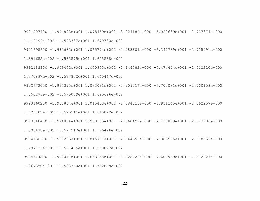
122
9991207400 -1.994893e+001 1.078469e+002 -3.024184e+000 -6.022639e+001 -2.737374e+000
1.412199e+002 -1.593337e+001 1.670730e+002
9991695600 -1.980682e+001 1.065774e+002 -2.983601e+000 -6.247739e+001 -2.725991e+000
1.391652e+002 -1.583575e+001 1.655588e+002
9992183800 -1.969462e+001 1.050963e+002 -2.944382e+000 -6.474444e+001 -2.712220e+000
1.370897e+002 -1.577852e+001 1.640467e+002
9992672000 -1.965395e+001 1.033021e+002 -2.909216e+000 -6.702081e+001 -2.700158e+000
1.350273e+002 -1.575069e+001 1.625626e+002
9993160200 -1.968834e+001 1.015403e+002 -2.884315e+000 -6.931145e+001 -2.692257e+000
1.329182e+002 -1.575141e+001 1.610822e+002
9993648400 -1.974854e+001 9.980165e+001 -2.860499e+000 -7.157809e+001 -2.683906e+000
1.308478e+002 -1.577917e+001 1.596426e+002
9994136600 -1.983236e+001 9.816721e+001 -2.844693e+000 -7.383586e+001 -2.678052e+000
1.287735e+002 -1.581485e+001 1.580027e+002
9994624800 -1.994011e+001 9.663168e+001 -2.828729e+000 -7.602969e+001 -2.672827e+000
1.267350e+002 -1.588360e+001 1.562048e+002

123
9995113000 -2.004565e+001 9.506959e+001 -2.809125e+000 -7.824432e+001 -2.665832e+000
1.246518e+002 -1.601442e+001 1.543782e+002
9995601200 -2.019018e+001 9.352750e+001 -2.792871e+000 -8.047071e+001 -2.660445e+000
1.225674e+002 -1.617921e+001 1.525700e+002
9996089400 -2.035042e+001 9.198404e+001 -2.780307e+000 -8.270508e+001 -2.657848e+000
1.204755e+002 -1.638533e+001 1.507281e+002
9996577600 -2.055563e+001 9.075974e+001 -2.772460e+000 -8.492853e+001 -2.659364e+000
1.183533e+002 -1.660760e+001 1.489901e+002
9997065800 -2.074644e+001 8.983188e+001 -2.770678e+000 -8.713496e+001 -2.662204e+000
1.162718e+002 -1.684722e+001 1.471181e+002
9997554000 -2.092867e+001 8.915650e+001 -2.771702e+000 -8.930810e+001 -2.672327e+000
1.141860e+002 -1.710550e+001 1.451243e+002
9998042200 -2.103799e+001 8.868250e+001 -2.771138e+000 -9.145021e+001 -2.679645e+000
1.121289e+002 -1.740034e+001 1.428768e+002
9998530400 -2.112583e+001 8.817115e+001 -2.771347e+000 -9.356522e+001 -2.692712e+000
1.100868e+002 -1.773140e+001 1.403258e+002

124
9999018600 -2.116773e+001 8.765734e+001 -2.766345e+000 -9.568748e+001 -2.697983e+000
1.080513e+002 -1.813193e+001 1.375023e+002
9999506800 -2.116063e+001 8.689763e+001 -2.758945e+000 -9.777220e+001 -2.705790e+000
1.060101e+002 -1.859782e+001 1.343736e+002
9999995000 -2.114283e+001 8.606619e+001 -2.746349e+000 -9.980790e+001 -2.710562e+000
1.040143e+002 -1.911402e+001 1.310208e+002
10000483200 -2.111561e+001 8.506052e+001 -2.744264e+000 -1.020508e+002 -
2.725312e+000 1.018804e+002 -1.977319e+001 1.271158e+002
10000971400 -2.107468e+001 8.397672e+001 -2.734247e+000 -1.041985e+002 -
2.739695e+000 9.980454e+001 -2.050254e+001 1.230231e+002
10001459600 -2.103452e+001 8.277034e+001 -2.730330e+000 -1.063288e+002 -
2.757500e+000 9.774010e+001 -2.132902e+001 1.183027e+002
10001947800 -2.093999e+001 8.140791e+001 -2.720279e+000 -1.084992e+002 -
2.780494e+000 9.570447e+001 -2.225273e+001 1.128561e+002
10002436000 -2.085586e+001 7.990858e+001 -2.713622e+000 -1.106523e+002 -
2.807003e+000 9.370177e+001 -2.325502e+001 1.066197e+002

125
10002924200 -2.079096e+001 7.833344e+001 -2.702918e+000 -1.128227e+002 -
2.828071e+000 9.174594e+001 -2.432952e+001 9.883500e+001
10003412400 -2.070745e+001 7.646339e+001 -2.696863e+000 -1.150069e+002 -
2.845854e+000 8.986693e+001 -2.535269e+001 8.931226e+001
10003900600 -2.066497e+001 7.464382e+001 -2.676817e+000 -1.172031e+002 -
2.849108e+000 8.800835e+001 -2.620315e+001 7.726466e+001
10004388800 -2.067926e+001 7.289611e+001 -2.657427e+000 -1.194526e+002 -
2.839993e+000 8.610764e+001 -2.671053e+001 6.268938e+001
10004877000 -2.072787e+001 7.138839e+001 -2.642978e+000 -1.217686e+002 -
2.815195e+000 8.413612e+001 -2.665287e+001 4.601712e+001
10005365200 -2.078213e+001 7.037801e+001 -2.630318e+000 -1.241547e+002 -
2.792984e+000 8.203975e+001 -2.601735e+001 3.023911e+001
10005853400 -2.079287e+001 7.007783e+001 -2.622703e+000 -1.265760e+002 -
2.773475e+000 7.986189e+001 -2.491346e+001 1.629474e+001
10006341600 -2.075246e+001 7.015565e+001 -2.625163e+000 -1.290096e+002 -
2.765133e+000 7.760550e+001 -2.363310e+001 5.151568e+000

126
10006829800 -2.060288e+001 7.052211e+001 -2.630555e+000 -1.314872e+002 -
2.766804e+000 7.531703e+001 -2.228909e+001 -3.724095e+000
10007318000 -2.037527e+001 7.085364e+001 -2.644888e+000 -1.339624e+002 -
2.772380e+000 7.307545e+001 -2.097273e+001 -1.070551e+001
10007806200 -2.007879e+001 7.095077e+001 -2.663668e+000 -1.364706e+002 -
2.779284e+000 7.082498e+001 -1.967251e+001 -1.641056e+001
10008294400 -1.974001e+001 7.090582e+001 -2.688922e+000 -1.390145e+002 -
2.779178e+000 6.853879e+001 -1.846660e+001 -2.159624e+001
10008782600 -1.936754e+001 7.095555e+001 -2.720986e+000 -1.415580e+002 -
2.784551e+000 6.615653e+001 -1.735441e+001 -2.625483e+001
10009270800 -1.894173e+001 7.089249e+001 -2.766097e+000 -1.441190e+002 -
2.795650e+000 6.370614e+001 -1.634562e+001 -3.053660e+001
10009759000 -1.846123e+001 7.064160e+001 -2.815098e+000 -1.466649e+002 -
2.824914e+000 6.120231e+001 -1.543145e+001 -3.452660e+001
10010247200 -1.794053e+001 7.026072e+001 -2.875136e+000 -1.492379e+002 -
2.859888e+000 5.867234e+001 -1.460460e+001 -3.815626e+001

127
10010735400 -1.737218e+001 6.957539e+001 -2.938832e+000 -1.517634e+002 -
2.910384e+000 5.618197e+001 -1.384959e+001 -4.145423e+001
10011223600 -1.678653e+001 6.852161e+001 -3.013395e+000 -1.542745e+002 -
2.967156e+000 5.368087e+001 -1.316378e+001 -4.448265e+001
10011711800 -1.619380e+001 6.712275e+001 -3.090793e+000 -1.567698e+002 -
3.034881e+000 5.120901e+001 -1.252610e+001 -4.727071e+001
10012200000 -1.560187e+001 6.551572e+001 -3.173349e+000 -1.592468e+002 -
3.107358e+000 4.876628e+001 -1.193639e+001 -4.990760e+001

128
REFERENCES
[1] Microlambda Wireless, available on web site http://www.microlambdawireless.com
[2] V. E. Demidov, B. A. Kalinikos, S. F. Karmanenko, A. A. Semenov, P. Edenhofer, “Electrical tuning of dispersion characteristics of surface electromagnetic-spin waves propagating in ferrite-ferroelectric layered structures,” IEEE Transactions on Microwave Theory and Techniques, vol. 51, no. 10, pp. 2090-2096, October 2003.
[3] H. How, P. Shi, C. Vittoria, E. Hokanson, M. H. Champion, L. C. Kempel, K. D. Trott, “Steerable phased array antennas using single-crystal YIG phase shifters – theory and experiments,” IEEE Transactions on Microwave Theory and Techniques, vol. 48, no. 9, pp. 1544-1549, September 2000.
[4] A. S. Tatarenko, G. Srinivasan, M. I. Bichurin, “Electrically-tunable microwave phase shifter based on ferrite-piezoelectric layered structure,” 18th Intl. Crimean Conference “Microwave & Telecommunication Technology”/IEEE, CFP08788, pp. 507, 508, September 2008.
[5] B. Foster, I. Gonin, T. Khabiboulline, A. Makarov, N. Solyak, I. Terechkine, and D. Wildman, “High power phase shifter,” Proceedings of 2005 Particle Accelerator Conference, Knoxville/IEEE 0-7803-8859-3/05, 0-7803-8859-3/05, pp. 3123-3125, 2005.
[6] M. Cohen, “An aligment technique for multiple ball YIG bandpass filters operating over multi-octave frequency bands,” Microwave Symposium Digest, IEEE-MTT-S International, pp. 33-36, 1978.
[7] G. Bryant, Principles of Microwave Measurements. Stevenage, United Kingdom: Peter Peregrinus Ltd., 1993.
[8] F. Ulaby, Electromagnetics for Engineers. Upper Saddle River, NJ: Pearson Prentice Hall, 2005.