yang-lee zeros of the yang-lee model - arxiv.org e … zeros of the yang-lee model g. mussardo,1,2...
TRANSCRIPT
Yang-Lee Zeros of the Yang-Lee Model
G. Mussardo,1, 2 R. Bonsignori,1 and A. Trombettoni3, 1
1SISSA and INFN, Sezione di Trieste, via Bonomea 265, I-34136, Trieste, Italy2International Centre for Theoretical Physics (ICTP), I-34151, Trieste, Italy
3CNR-IOM DEMOCRITOS Simulation Center, Via Bonomea 265, I-34136 Trieste, Italy
To understand the distribution of the Yang-Lee zeros in quantum integrable field theories we analysethe simplest of these systems given by the two-dimensional Yang-Lee model. The grand-canonicalpartition function of this quantum field theory, as a function of the fugacity z and the inversetemperature β, can be computed in terms of the Thermodynamics Bethe Ansatz based on its exactS-matrix. We extract the Yang-Lee zeros in the complex plane by using a sequence of polynomialsof increasing order N in z which converges to the grand-canonical partition function. We showthat these zeros are distributed along curves which are approximate circles as it is also the case ofthe zeros for purely free theories. There is though an important difference between the interactivetheory and the free theories, for the radius of the zeros in the interactive theory goes continuouslyto zero in the high-temperature limit β → 0 while in the free theories it remains close to 1 even forsmall values of β, jumping to 0 only at β = 0.
Pacs numbers: 11.10.St, 11.15.Kc, 11.30.Pb
I. INTRODUCTION
Many physical quantities reveal their deeper structure by going to the complex plane. This is the case,for instance, of the analytic properties of the scattering amplitudes where the angular momentum is notlonger restricted to be an integer but allowed to take any complex value giving rise in this way to thefamous Regge poles [1]. Another famous example is the Yang-Lee theory of equilibrium phase transitions[2, 3] based on the zeros of the grand-canonical partition function in the complex plane of the fugacity:in a nutshell, the main observation of Yang and Lee was that the zeros of the grand-canonical partitionfunctions in the thermodynamic limit usually accumulate in certain regions or curves of the complexplane, with their positive local density η(z) which changes by changing the temperature; if at a criticalvalue Tc, the zeros accumulate and pinch a positive value of the real axis, this is what may mark theonset of a phase transition.
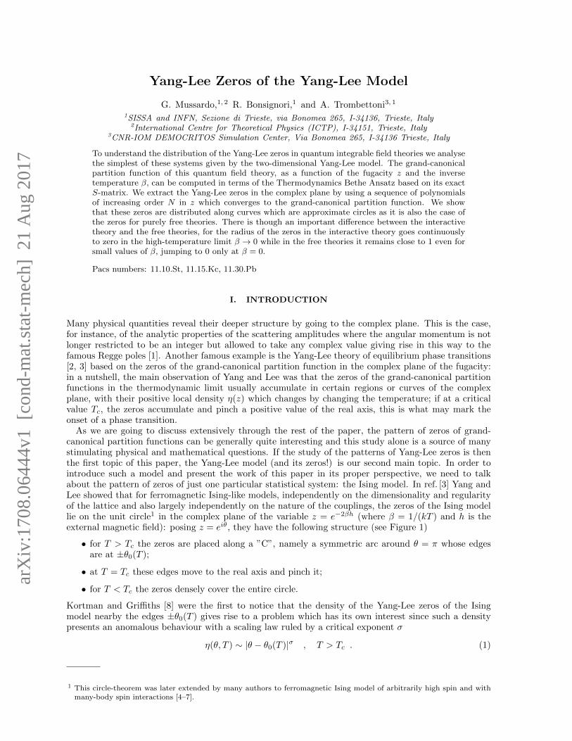
As we are going to discuss extensively through the rest of the paper, the pattern of zeros of grand-canonical partition functions can be generally quite interesting and this study alone is a source of manystimulating physical and mathematical questions. If the study of the patterns of Yang-Lee zeros is thenthe first topic of this paper, the Yang-Lee model (and its zeros!) is our second main topic. In order tointroduce such a model and present the work of this paper in its proper perspective, we need to talkabout the pattern of zeros of just one particular statistical system: the Ising model. In ref. [3] Yang andLee showed that for ferromagnetic Ising-like models, independently on the dimensionality and regularityof the lattice and also largely independently on the nature of the couplings, the zeros of the Ising modellie on the unit circle1 in the complex plane of the variable z = e−2βh (where β = 1/(kT ) and h is theexternal magnetic field): posing z = eiθ, they have the following structure (see Figure 1)
• for T > Tc the zeros are placed along a ”C”, namely a symmetric arc around θ = π whose edgesare at ±θ0(T );
• at T = Tc these edges move to the real axis and pinch it;
• for T < Tc the zeros densely cover the entire circle.
Kortman and Griffiths [8] were the first to notice that the density of the Yang-Lee zeros of the Isingmodel nearby the edges ±θ0(T ) gives rise to a problem which has its own interest since such a densitypresents an anomalous behaviour with a scaling law ruled by a critical exponent σ
η(θ, T ) ∼ |θ − θ0(T )|σ , T > Tc . (1)
1 This circle-theorem was later extended by many authors to ferromagnetic Ising model of arbitrarily high spin and withmany-body spin interactions [4–7].
arX
iv:1
708.
0644
4v1
[co
nd-m
at.s
tat-
mec
h] 2
1 A
ug 2
017
2
FIG. 1: Distribution of the Yang-Lee zeros for the Ising model in the complex plane of the fugacity z.
Such a behavior is closely analogous to the usual critical phenomena (although in this case triggeredby a purely imaginary magnetic field ih) and therefore Fisher [9] posed the question about its effectivequantum field theory and argued that, in sufficiently high dimension d, this consists of a φ3 Landau-Ginzburg theory for the scalar field φ(x) with euclidean action given by
A =
∫ddx
[1
2(∂φ)2 + i(h− h0)φ+ ig φ3
]. (2)
This action is what defines the Yang-Lee model, i.e. the quantum field theory studied in this paper, andthe imaginary couplings present in such an action is what makes the Yang-Lee model a non-hermitiantheory; the theory is however invariant under a CP transformations [10, 12] and therefore its spectrumis real. At criticality, i.e. when h = h0, the corresponding fixed point of the Renormalization Grouppresents only one relevant operator, namely the field φ(x) itself: in two dimensions Cardy showed [11]that all these properties are encoded into the simplest non-unitarity minimal model of Conformal FieldTheories which has central charge c = −22/5 and only one relevant operator of conformal dimension∆ = −1/5. Still in two dimensions, Cardy and Mussardo [10] then argued that the action (2), regardedas deformation of this minimal conformal model by means of its relevant operator φ(x) corresponds to anintegrable quantum field theory. This fact has far-reaching consequences: indeed, the infinite number ofconservation laws – the fingerprint of any integrable field theory [14–16] – implies that scattering processesof the Yang-Lee model are completely elastic and factorizable in terms of the two-body scattering matrixwhich was exactly computed in [10]. The spectrum can be easily extracted by the poles of the S-matrixand turns out to consist of only one massive particle which may be regarded as a bound state of itself.Exact Form Factors and two-point correlation functions of this massive model were later computed anddiscussed in [13].
Based on the S-matrix scattering theory and the Thermodynamic Bethe Ansatz introduced by Al.B.Zamolodchikov [17], one can then in principle determine exactly (although numerically) the free-energyof the integrable models as function of the inverse temperature β and the fugacity z [19, 20]. This isindeed what we have done in this paper for the Yang-Lee model, i.e. one of the simplest representativeof integrable quantum field theories, for the purpose of studying what kind of distribution emerges forthe zeros of the grand-canonical partition function of these systems. We hope these brief introductoryconsiderations were useful to clarify the general aims of this paper and the ”recursive” use of Yang-Leenames, both to denote the zeros and the eponymous model, and the zeros of the model itself!
A comment is in order on the logic of this work. In the Yang-Lee theory of phase transitions one relatesthermodynamical properties, such the free energy and the magnetization, to the density of Yang-Lee zerosη(z). Usually the focus is on the (often approximate) determination of η(z) in order then to extract theequilibrium quantities of interest. However, the point of view we adopt to deal with integrable quantumfield theories as, for instance the Yang-Lee model, is rather the opposite, since the free energy of thesemodels are already known in terms of the Thermdoynamics Bethe Ansatz equations, and this gives thepossibility to determine the properties of the zeros. We have applied such a procedure to the Yang-Lee
3
model but it is clear that it can be applied as well to other integrable quantum field theories.The rest of the paper is organised as follows. Section II is devoted to a brief recap of the main points
of the Yang-Lee theory of the phase transition and the importance to control the distribution of the zerosof the grand-canonical partition function in order to study the thermodynamics. Section III contains adetailed discussion on the nature of the roots of polynomials which may be regarded as grand-canonicalpartition functions of some appropriate physical system. In Section IV we present the closed formulas ofthe partition functions of free bosonic and fermionic theories, both in the non-relativistic and relativisticcase, and also in the presence of an harmonic trap. Sections V and VI contain a detailed discussion ofthe zeros of the grand-canonical partition functions of the non-relativistic and relativistic free theoriesrespectively: apart from some peculiar features emerging from this study, the basic purpose of theseSections is to set the stage for the analysis of the interacting integrable models discussed in the laterSections. In particular, in Section VII we start recalling the basic properties of integrable quantum fieldtheories, namely the S-matrix formulation and the Thermodynamics Bethe Ansatz which allows us torecover the partition function of the integrable models. In Section VIII we study in detail the Yang-Leezeros of the simplest quantum integrable field theories, namely the Yang-Lee model. Our conclusions arefinally collected in Section IX.
II. YANG-LEE THEORY OF PHASE TRANSITIONS
In order to overcome some inadequacies of the Mayer method [21] for dealing with the condensation of agas and also to understand better the underlying mathematical reasons behind the occurrence of phasetransitions, in 1952 Yang and Lee proposed to analytically continue the grand-canonical partition functionto the complex plane of its fugacity and determine the pattern of zeros of this function. Although only realvalues of the fugacity determine the physical value of the pressure, the magnetization or other relevantthermodynamical quantities, the overall analytic behavior of these observables can only be understoodby looking at how the zeros move as a function of an external parameter such as the temperature. Inthis Section we are going to simply write down, mainly for future reference, the basic formulas of theYang-Lee formalism with few extra comments.
Concerning general references on this topic, in addition to the original papers [2, 3] and others previouslymentioned [4–11], the reader may also benefit of some standard books [22, 23] or reviews such as [24, 25]and references therein. As a matter of fact, the literature on the subject is immense, even ranging acrossseveral fields of physics and mathematics. For this reason we cannot definitely do justice to all authorswho contributed to the development of the subject but we would like nevertheless to explicitly mentionfew more references which we have found particularly useful, such as the series of papers by Ikeda [26–28]or by Abe [29, 30], the papers by Katsura on some analytic expressions of the density of zeros [5], thepaper by Fonseca and Zamolodchikov [32] on the analytic properties of the free energy of the Ising fieldtheory and some related references on this subject such as [17, 18, 33–36], and finally some references onthe experimental observations of the Yang-Lee zeros [37], in particular those based on the coherence of aquantum spin coupled to an Ising-type thermal bath [38, 39].
Yang-Lee formulation. Consider for simplicity the grand-canonical partition function ΩN (z) of a gasmade of N particles with hard cores b in a volume V , of activity z and at temperature T is given by
ΩN (z) =
N∑k=0
1
k!Zk(V, T )zk =
N∏l=1
(1− z
zl
), (3)
where N = V/b is the largest number of particles that can be contained in the volume, the coefficientsZk(V, T ) are the canonical partition functions of a system of k particles and the z is the fugacity. As apolynomial of order N , ΩN (z) has z1, z2, . . . zN zeros in the complex plane. The thermodynamics of thesystem is recovered by defining, in the limit V →∞, the pressure p(z) and the density ρ(z) of the systemas
p(z)
kT≡ f(z) = lim
V→∞
1
Vlog ΩN (z) = lim
V,N→∞
1
V
N∑l=1
log
(1− z
zl
), (4)
ρ(z) ≡ zf ′(z) = limV→∞
1
Vzd
dzlog ΩN (z) = lim
V,N→∞
1
V
N∑l=1
z
z − zl. (5)
4
For extended systems the limit V → ∞ also enforces N → ∞ and therefore there will be an infinitenumber of zeros: these may become densely distributed in the complex plane according to their positivedensity function η(z), which can be different from zero either in a region A of the complex plane (such asituation we will call later area law for the zeros) or along a curve, C (to which we refer to as a perimeterlaw). Apart from these two generic cases, it can also be that the zeros may remain isolated points in thecomplex plane or, rather pathologically, accumulated instead around single points.
As shown in the original papers by Yang and Lee [2, 3], the entire thermodynamics can be recoveredin terms of the density η(z) of the zeros of the grand-canonical partition function. Notice that, for thereality of the original ΩN (z), this function must satisfy the property
η(z) = η(z∗) , (6)
i.e. must be symmetric with respect to the real axis. The region A or the curve C depend on thetemperature T and they change their shape by changing T . Let’s initially assume that the zeros areplaced on an extended area A: in this case, for all points outside this region one can analytically extendthe definition of the pressure p(z) as
p(z)
kT=
∫A
dξ η(ξ) log
(1− z
ξ
). (7)
We can split this function into its real and imaginary part
p(z)
kT≡ P (z) = ϕ(z) + iψ(z) , (8)
where its real part
ϕ(z) =
∫dξ η(ξ) log
∣∣∣∣1− z
ξ
∣∣∣∣ (9)
involves log |z|, i.e. the Green function of the two-dimensional Laplacian operator ∆. Therefore ϕ(z)satisfies the Poisson equation
∆ϕ(z) = 2π η(z) . (10)
Drawing an electromagnetic analogy, this equation implies that ϕ(z) can be thought as the electrostaticpotential generated by the the (positive) distribution of charges with density η(z). Posing z = x + iy,the corresponding components of the electric field are given by
E1 = −∂ϕ∂x
, E2 = −∂ϕ∂y
. (11)
Since in any region not occupied by the charges both ϕ(z) and its companion ψ(z) are analytic functionsrelated by the Cauchy-Riemann equations, we have
dP
dz=
dϕ
dx+ i
dψ
dx=dϕ
dx− idψ
dy= −E , (12)
where E = E1 + iE2 is the complex electric field (E = E1 − iE2).This electrostatic analogy is pretty appealing but it is important to realise that not all charge den-
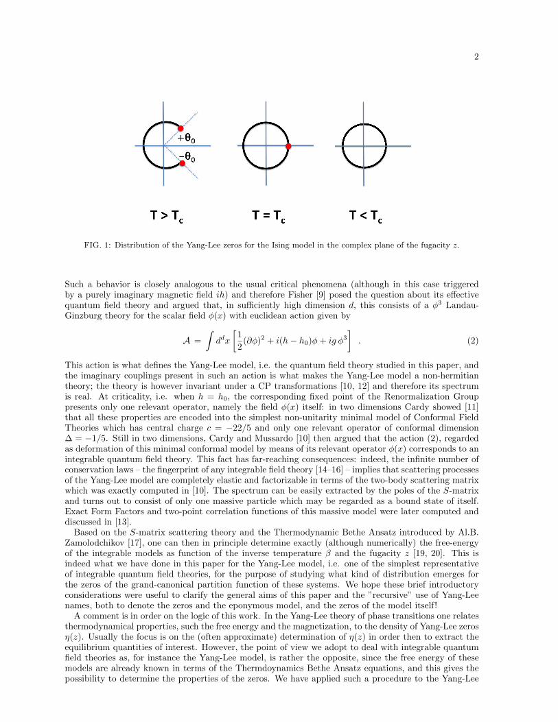
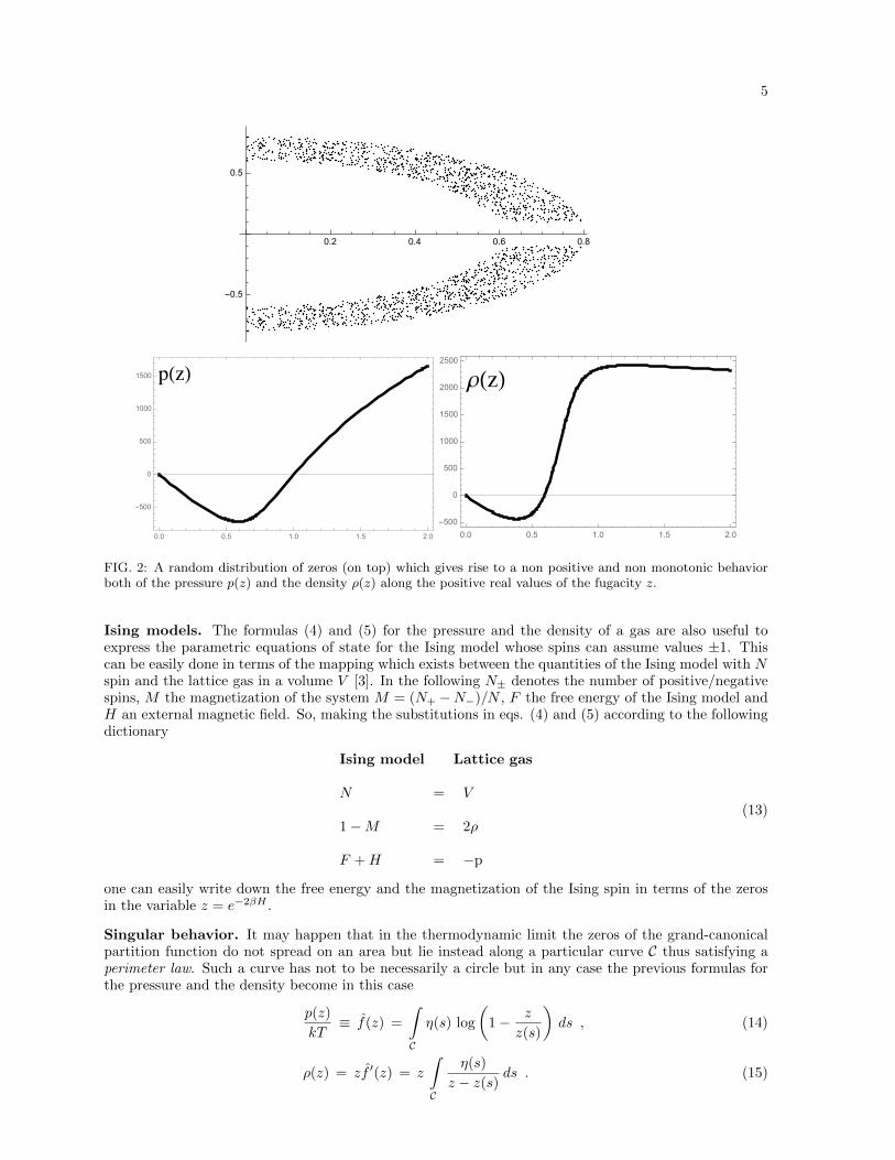
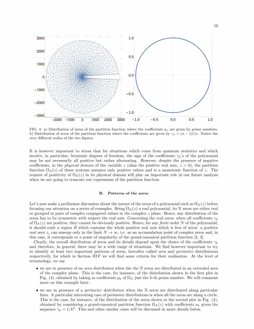
sities are appropriate for the statistical mechanics problem. For this purpose, there are indeed certainrequirements to fulfil, such as: its pressure p(z), computed according to eq. (4), must be necessarily acontinuous and positive function of z, monotonically increasing, along the real axis of the variable z; atthe same time, its density ρ(z), computed according to eq. (5), must also be a positive but not necessarilya continuous function, increasing too along the real axis of z. It may be stressed that these conditionsalone may be not sufficient to define a physical systems but if they are violated the system at hand issurely unphysical. For instance, for the random distributions of zeros shown in the top of Figure 2, thecorresponding pressure and density, shown on the bottom of the same figure, do not fulfil the physicalconditions of positivity and monotonicity: therefore, this set of zeros shown does not correspond to anyphysical statistical system. We will come back again to this issue later at the end of this Section.
5
()
0.0 0.5 1.0 1.5 2.0
-500
0
500
1000
1500 ρ()
0.0 0.5 1.0 1.5 2.0
-500
0
500
1000
1500
2000
2500
FIG. 2: A random distribution of zeros (on top) which gives rise to a non positive and non monotonic behaviorboth of the pressure p(z) and the density ρ(z) along the positive real values of the fugacity z.
Ising models. The formulas (4) and (5) for the pressure and the density of a gas are also useful toexpress the parametric equations of state for the Ising model whose spins can assume values ±1. Thiscan be easily done in terms of the mapping which exists between the quantities of the Ising model with Nspin and the lattice gas in a volume V [3]. In the following N± denotes the number of positive/negativespins, M the magnetization of the system M = (N+ −N−)/N , F the free energy of the Ising model andH an external magnetic field. So, making the substitutions in eqs. (4) and (5) according to the followingdictionary
Ising model Lattice gas
N = V
1−M = 2ρ
F +H = −p
(13)
one can easily write down the free energy and the magnetization of the Ising spin in terms of the zerosin the variable z = e−2βH .
Singular behavior. It may happen that in the thermodynamic limit the zeros of the grand-canonicalpartition function do not spread on an area but lie instead along a particular curve C thus satisfying aperimeter law. Such a curve has not to be necessarily a circle but in any case the previous formulas forthe pressure and the density become in this case
p(z)
kT≡ f(z) =
∫C
η(s) log
(1− z
z(s)
)ds , (14)
ρ(z) = zf ′(z) = z
∫C
η(s)
z − z(s)ds . (15)
6
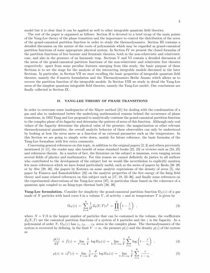
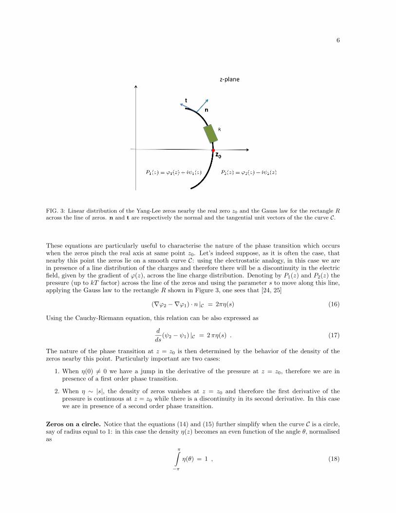
FIG. 3: Linear distribution of the Yang-Lee zeros nearby the real zero z0 and the Gauss law for the rectangle Racross the line of zeros. n and t are respectively the normal and the tangential unit vectors of the the curve C.
These equations are particularly useful to characterise the nature of the phase transition which occurswhen the zeros pinch the real axis at same point z0. Let’s indeed suppose, as it is often the case, thatnearby this point the zeros lie on a smooth curve C: using the electrostatic analogy, in this case we arein presence of a line distribution of the charges and therefore there will be a discontinuity in the electricfield, given by the gradient of ϕ(z), across the line charge distribution. Denoting by P1(z) and P2(z) thepressure (up to kT factor) across the line of the zeros and using the parameter s to move along this line,applying the Gauss law to the rectangle R shown in Figure 3, one sees that [24, 25]
(∇ϕ2 −∇ϕ1) · n |C = 2πη(s) (16)
Using the Cauchy-Riemann equation, this relation can be also expressed as
d
ds(ψ2 − ψ1) |C = 2πη(s) . (17)
The nature of the phase transition at z = z0 is then determined by the behavior of the density of thezeros nearby this point. Particularly important are two cases:
1. When η(0) 6= 0 we have a jump in the derivative of the pressure at z = z0, therefore we are inpresence of a first order phase transition.
2. When η ∼ |s|, the density of zeros vanishes at z = z0 and therefore the first derivative of thepressure is continuous at z = z0 while there is a discontinuity in its second derivative. In this casewe are in presence of a second order phase transition.
Zeros on a circle. Notice that the equations (14) and (15) further simplify when the curve C is a circle,say of radius equal to 1: in this case the density η(z) becomes an even function of the angle θ, normalisedas
π∫−π
η(θ) = 1 , (18)
7
and the pressure and density are expressed as
p(z)
kT=
π∫0
η(θ) log(z2 − 2z cos θ + 1) dθ , (19)
ρ(z) = 2z
π∫0
η(θ)z − cos θ
z2 − 2z cos θ + 1dθ . (20)
For a circle distribution of the zeros, it is easy to find a condition on the density η(θ) which ensuresthat both the pressure and the density are positive monotonic functions of z: as shown in [26], it is infact sufficient that the density η(θ) is bounded and continuous, while its derivative η′(θ) is a bounded,continuous and positive function. Indeed, taking the derivative of ρ(z) with respect to z we have
dρ
dz= 2
π∫0
η(θ)2z − (1 + z2) cos θ
(z2 − 2z cos θ + 1)2dθ , (21)
which, with the change of variable ξ = tan(θ/2) and an integration by part, can be expressed as
dρ
dz= −4
[ξ η(2 arctan ξ)
(z + 1)2ξ2 + (z − 1)2
]∞0
+ 8
π∫0
ξ η′(2 arctan ξ)
(1 + ξ)2((z + 1)2ξ2 + (z − 1)2dξ . (22)
With the hypothesis that η(θ) is a bounded function, the first term of this expression vanishes while thesecond term, as far as η′(θ) > 0, is positive. Once established that the function ρ(z) is then an increasingmonotonic function, to show that it is always positive is sufficient to calculate its value at the origin and,if not negative, the function ρ(z) will be indeed always positive. Since at z = 0 we have ρ(0) = 0, this issufficient to show the positivity of ρ(z).
Under the same hypothesis for η(θ), we can also conclude that the pressure p(z) is a positive andincreasing function of z: since
ρ(z) = zdp
dz=
dp
d log z, (23)
the positivity of ρ(z) implies that p(z) is an increasing function of log z, i.e. of z itself since the logarithmicfunction is a monotonic function. So, also for p(z) to prove that this is always a positive function it issufficient to compute its value at the origin and check that it is not negative. Since p(0) = 0, thisconcludes the argument.
The importance of these considerations becomes more clear once one realises that even assuming themost favourable distribution of the zeros, i.e. along a circle, the analytic expression of the densities η(θ)is largely unknown. The very few cases where we have such an information include the one-dimensionalIsing model with nearest-neighbor interaction [3] and various versions of the mean field solutions of thesame model [31]. As a further intriguing remark, it seems that if one is able to point out what arethe conditions in order to have a proper physical density η(θ), there is a plenty of room to define newstatistical model by inverting somehow the theory of Yang and Lee. We will further comment on thispoint in the conclusions of the paper.
Yang-Lee edge singularities. We can take advantage of the known expression of the density of zerosof the one-dimensional ferromagnetic Ising model for presenting the simplest example of Yang-Lee edgesingularities. The absence of a phase transition in this one-dimensional model of course implies that η(θ)must vanish in an interval around the origin. This is indeed the case and the exact expression of thedistribution is given by [3]
η(θ) =1
2π
sin θ2√
sin2 θ2 − sin2 θ0
2
, if |θ| > θ0 (24)
otherwise 0, where θ0 = arccos(1 − 2e−2βJ) and J is the coupling constant between two next-neighborspins. The zeros take then the C-shape of the plot on the left in Figure 1. In this example θ0 plays
8
the role of an edge singularity and this value pinches the origin only when βJ → ∞, namely at T = 0.Nearby θ0 the density of zeros behaves anomalously as
g(θ) ∼ C√θ − θ0
, (25)
(C = 1/(2π)√
tan θ02 ), therefore for the one-dimensional Ising model the Yang-Lee edge singularity expo-
nent defined in eq. (1) is equal to σ = −1/2. Consider now the expression of the magnetization in termsof the density of the zeros using the dictionary previously established
M(z) = 1− 4z
π∫0
η(θ)z − cos θ
z2 − 2z cos θ + 1dθ . (26)
Performing the integral we have
M(z) =z − 1√
(z − eiθ0) (z − e−iθ0). (27)
Posing z = e−2βh and θ0 = −2βhc, and expanding this formula around h = ihc, we have
M(h) ∼ M0
(h− ihc)1/2, (28)
i.e. the value ihc can be considered as a singular point.
Polynomials vs Series. The discussion made so far concerned with the singular behavior which emergesby increasing the order N of a sequence of genuine polynomials, in particular when N → ∞. But whatabout is the partition function Ω(z) is ab-initio given in terms not of a polynomial but an infinite series?Let’s say Ω(z) in a neighborough of z = 0 is given by the infinite series
S(z) =
∞∑k=0
αnzn . (29)
In this case one must be aware that analysing the Yang-Lee zeros of an expression such as in eq. (29)there may be a condensation of zeros along some positive value z0 of the fugacity z which however doesnot necessarily signal a phase transition of the physical system but rather the finite radius of convergenceof the series itself! Imagine in fact that the series (29) could be analytically continued and that thecorresponding function Ω(z) has the closest singularity nearby the origin at a negative value z = −R.This automatically fixes the radius of convergence of the series (29) to be R and therefore if we woulduse such a series to define the partition function, the corresponding Yang-Lee zeros may also condensateat the positive value z = R, even though this point is not associated to a phase transition of the actualfunction Ω(z). A simple example of this phenomena is worked out in detail in Appendix A. We will seethat similar cases also emerge in discussing the Yang-Lee zero distributions of fermionic theories whosecorresponding series S(z) has alternating sign and therefore a singularity at a negative value of z: theirzeros however also condensate at a positive real value of z.
III. PLAYING WITH POLYNOMIALS
In this Section we are going to deal extensively with the properties of the main mathematical object ofthis paper, namely the class of real polynomials ΩN (z) of order N in the variable z
ΩN (z) = γ0 + γ1z + γ2 z2 + . . . γN z
N . (30)
The coefficients γn of these polynomials are real and we choose hereafter γ0 = 1. Since we are going tointerpret ΩN (z) as a generalised grand-canonical partition function of a statistical model, either classicalor quantum, we pose
ΩN (z) ≡ eFN (z) , (31)
9
where we have define the so-called free-energy FN (z) of the system, directly related to the pressure ofthe system, see eq. (4). In light of this statistical interpretation of ΩN (z) in the following we will alsoexpress it with a different normalization of the coefficients
ΩN (z) =
N∑k=0
akk!zk , (32)
with γk = ak/k! and a0 = 1 while the higher coefficients ak’s assume the familiar meaning of canonicalpartition functions of k particles. Formulas which we derive below are sometimes more elegantly expressedin terms of the ak’s although we will switch often between the two equivalent expressions (30) and (32),hoping that this will not confuse the reader.
A. Sign of the coefficients
For models coming from classical statistical physics, it is easy to argue that the coefficients ak of therelative polynomial ΩN (z) are generically all positive, ak > 0. In this respect, consider for instance twosignificant examples:
• Classical Gas. A classical model of a gas in d-dimension, made of N particles of mass m andHamiltonian of the form
H =
N∑i=1
p2i
2m+∑i,j
u(rij) , (33)
where rij is the distance between the i-th and j-th particle. In this case the grand-canonicalpartition function of the system assumes the form (32), where the variable z expressed by
z = eβµ(2πmβ/h2
) d2 , (34)
where µ is the fugacity, β = 1/kT where T is the temperature and h is the Planck constant hereintroduced to normalise the phase-space integral. Therefore in this example the coefficients ak aregiven the positive integrals
ak =
∫· · ·∫dr1 · · · drk exp
−β∑i,j
u(rij)
> 0 . (35)
• Ising in a magnetic field. As a second example of classical statistical mechanics, consider theferromagnetic Ising model in a magnetic field H studied originally by Lee and Yang in [3]: in thiscase, with σi = ±1 and a general two-body ferromagnetic Hamiltonian of N spins in a regularlattice in arbitrary d-dimensional lattice of the form
H = −∑i,j
Jijσiσj −H∑i
σi , Jij > 0 (36)
posing
z = e−2βH , (37)
the partition function of the model is expressed by a palindrome polynomial in this variable, i.e. apolynomial of the form (30) where the coefficients satisfy the additional condition
γk = γN−k > 0 . (38)
This because γk is the contribution to the partition function of the Ising model in zero magneticfield coming from configurations in which the number N− of spins σi = −1 is equal to k; thiscontribution is evidently the same also for N− = (N − k).
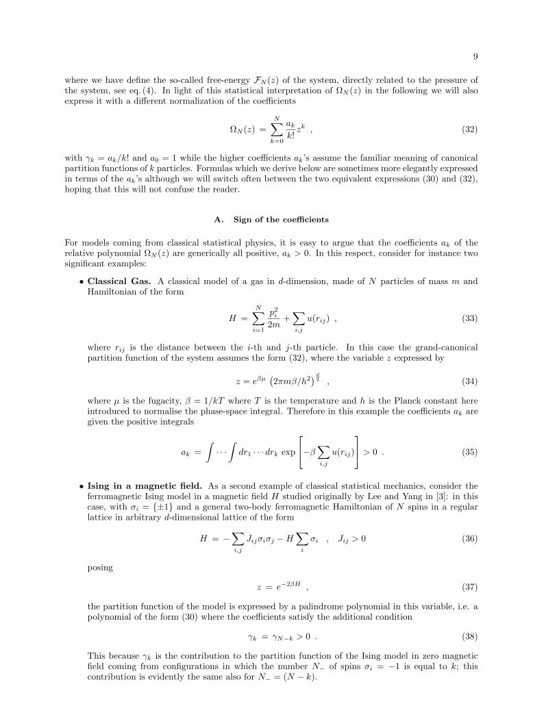
10
-1.0 -0.5 0.0 0.5 1.0
-1.0
-0.5
0.0
0.5
1.0
FIG. 4: a) Distribution of zeros of the partition function where the coefficients an are given by prime numbers.b) Distribution of zeros of the partition function where the coefficients are given by γn = (n− 1)!/n. Notice thevery different scales of the two figures.
It is however important to stress that for situations which come from quantum statistics and whichinvolve, in particular, fermionic degrees of freedom, the sign of the coefficients γk’s of the polynomialmay be not necessarily all positive but rather alternating. However, despite the presence of negativecoefficients, in the physical domain of the variable z (alias the positive real axis, z > 0), the partitionfunction ΩN (z) of these systems assumes only positive values and is a monotonic function of z. Therequest of positivity of ΩN (z) in its physical domain will play an important role in our future analysiswhen we are going to truncate our expressions of the partition function.
B. Patterns of the zeros
Let’s now make a preliminar discussion about the nature of the zeros of a polynomial such as ΩN (z) beforefocusing our attention on a series of examples. Being ΩN (z) a real polynomial, its N zeros are either realor grouped in pairs of complex conjugated values in the complex z plane. Hence, any distribution of thezeros has to be symmetric with respect the real axis. Concerning the real zeros, when all coefficients γkof ΩN (z) are positive, they cannot be obviously positive. Hence, for any finite order N of the polynomial,it should exist a region R which contains the whole positive real axis which is free of zeros: a positivereal zero zc can emerge only in the limit N →∞, i.e. as an accumulation point of complex zeros and, inthis case, it corresponds to a point of singularity of the grand-canonical partition function [2, 3].
Clearly, the overall distribution of zeros and its details depend upon the choice of the coefficients γkand therefore, in general, there may be a wide range of situations. We find however important to tryto identify at least two important patterns of zeros, hereafter called area and perimeter distributionsrespectively, for which in Section III F we will find some criteria for their realisation. At the level ofterminology, we say
• we are in presence of an area distribution when the the N zeros are distributed in an extended areaof the complex plane. This is the case, for instance, of the distribution shown in the first plot inFig. (4), obtained by taking as coefficients pk of ΩN just the k-th prime number. We will commentmore on this example later.
• we are in presence of a perimeter distribution when the N zeros are distributed along particularlines. A particular interesting case of perimeter distributions is when all the zeros are along a circle.This is the case, for instance, of the distribution of the zeros shown in the second plot in Fig. (4),obtained by considering a grand-canonical partition function ΩN (z) with coefficients ak given thesequence γk = 1/k2. This and other similar cases will be discussed in more details below.
11
C. Bounds on the absolute module of the zeros
Given a polynomial of the form (30), there are several bounds on the magnitudes |zi| of its roots. Herewe simply state some of these bounds without any proof for them (it may be useful to consult the bookby Prasolov [40] as a general reference on polynomials and bounds on their roots). Some of these boundsare more stringent than others (and we list them in the order of increasing their level of refinement) butaltogether they may help in getting an idea about the distribution of the roots.
• Cauchy bound. The Cauchy bound states that the roots zi have an absolute value less than RC ,|zi| < RC , where
RC = 1 +1
|γN |max |γ0|, |γ1|, . . . |γN−1| . (39)
This is usually the less stringent bound on the module on the roots.
• Sun-Hsieh bound. The Cauchy bound can be refined in terms of the Sun-Hsieh bound, |zi| <RSH , where
RSH = 1 +1
2
((|γN−1/γN | − 1) +
√(|γN−1/γN | − 1)2 + 4a
), a = max|γk/γN | . (40)
• Fujiwara bound. A further refinement comes from the Fujiwara bound where all roots are withinthe disc of radius RF , |zi| < RF , where
RK = 2 max
∣∣∣∣γN−1
γN
∣∣∣∣ , ∣∣∣∣γN−2
γN
∣∣∣∣ 12 , · · · , ∣∣∣∣ γ1
γN
∣∣∣∣ 1N−1
,1
2
∣∣∣∣ γ0
γN
∣∣∣∣ 1N
. (41)
• Enestrom bounds. When all γk > 0, we can have a lower and an upper bound of the magnitudeof the roots given by
Rd ≤ |zi| ≤ Ru , (42)
where
Rd = min
γkγk+1
, Ru = max
γkγk+1
, k = 0, 1, . . . N − 1 . (43)
The Enestrom bounds are usually the best estimate of the annulus in the complex plane where theroots are located.
• Enestrom-Kakeya bound. Let us also mention the Enestrom-Kakeya bound which refers topolynomials where the coefficients γk satisfy the condition
γ0 ≤ γ1 ≤ γ2 . . . ≤ γN . (44)
In this case we have that |zi| ≤ (|γN | − γ0 + |γ0|)/|γN |. In particular, if all coefficients γk arepositive, the roots are within the unit disc, |zi| ≤ 1. Of course, when the coefficients satisfy insteadthe condition
γ0 ≥ γ1 ≥ γ2 . . . ≥ γN . (45)
when |zi| ≥ 1.
Let’s make a final comment on the information provided by the bounds on the modules of the zeros:these bounds refer to all roots, so if knew for instance that |zi| < 100, it may happen that just one orfew zeros has module |z| ∼ 100 while all the rest may have a very small module. In other words, boundsusually refer to the largest of the zeros rather than their overall distribution.

12
D. Motion of the zeros: perturbative analysis
We can study how the distribution of the zeros of a polynomial is modified by the addition of a new rootas the order of the polynomial is increased by 1. To this aim, consider a polynomial of the form
ΩN (x) = ΩN−1(x) + γNxN . (46)
The addition of the new term γNxN to ΩN−1(x) has two effects:
1. it creates a new zero;
2. it moves the previous ones.
Let us address the first issue by considering the equation for the zeros of the new polynomial
ΩN−1(x) + γNxN = 0 . (47)
Writing it as
x = −ΩN−1(x)
γNxN−1= −γN−1
γN− γN−2
γN−1x+ . . . , (48)
we see that, perturbatively in aN , the new root x∗ is roughly placed at
x∗ ' −γN−1
γN. (49)
If γN is infinitesimally small with respect to the other previous coefficients, the value x∗ determined fromthis equation is large and therefore, self-consistently, it is justified to neglect its corrections coming fromthe inverse powers (1/x∗)l present in the left hand side of (48).
Let us now address the second issue, i.e. the motion of the other zeros, once again perturbatively inthe quantity aN . Let xi (i = 1, . . . , N − 1) be one of the zeros of the polynomial PN−1(x). Let’s nowwrite
xi + δxi (50)
as the new position of the root, once the new term aNxN has been added
ΩN (xi + δxi) = ΩN−1(xi + δxi) + γN (xi + δxi)N = 0
= ΩN−1(xi) + δxidΩN−1
dxi+ γNx
Ni +NγNx
N−1i δxi =
= δxi
[dΩN−1
dxi+NγNx
N−1i
]+ γNx
Ni = 0 , (51)
hence the displacement of the i− th root due to the addition on the term aNxN is given by
δxi = − γNxNi(
dZN−1
dxi+ γNNx
N−1i
) . (52)
E. Statistical approach
In order to understand better the pattern of the zeros and, in particular, to see whether we are able toqualitatively predict if an area or a perimeter law occurs, it is worth setting up a statistical analysis ofthe zeros. The obvious quantities to look at are the statistical moments sk of the zeros defined as
sk ≡N∑l=1
zkl , (53)

13
where k can be either a positive or a negative integer. Notice that, being the polynomial real, all sk arereal quantities.
Negative moments. Let’s see how to relate the negative moments of the zeros
s−m ≡ sm =
N∑l=1
(1
zl
)m, (54)
to the coefficients of the polynomial ΩN (z). In order to do so, let’s factorise the partition functions interms of its zeros as
ΩN =
N∏l=1
(1− z
zl
). (55)
Taking the logarithm of both sides we arrive to the familiar cluster expansion of the free-energy FN (z)
FN (z) = log ΩN (z) =
N∑l=1
log
(1− z
zl
)= −
N∑l=1
∞∑m=1
1
m
(z
zl
)m=
≡∞∑m=1
bmzm .
The negative moments sm are then related to the cluster coefficients bm as [2]
bm = − 1
m
N∑l=1
(1
zl
)m= − 1
msm . (56)
It is also custom to expand the free-energy FN (z) in terms of the cumulants ck defined by
FN (z) = ln ΩN ≡∞∑k=1
ckk!zk . (57)
If we use for Ω(z) the expression (32) and the coefficients ak, the cumulants are given by
c1 = a1
c2 = a2 − a21
c3 = a3 − 3a2a1 + 2a31
...
(58)
As a matter of fact there exists a closed formula which relates the two sets of coefficients ck and ak.To this aim let’s introduce the determinant of a (k × k) matrix M(k) whose entries involve the first kcoefficients al (l = 1, 2, . . . k)
M(k) =
a1 1 0 · · · 0
a2 a1 1...
a3 a2
(21
)a1 0
......
......
ak ak−1
(k1
)ak−2 · · ·
(k−1k−2
)a1
. (59)
The final formula is then
ck = (−1)k−1 detM(k) . (60)
The relevant thing to note is that the k-th cluster coefficient ck, which is of course related to the k-thmoment of the inverse roots as
ck = −(k − 1)! sk , (61)
14
is entirely determined only by the first k coefficients of the original polynomial ΩN . This implies that, ifwe increase the order N → N + N of the polynomial by adding to ΩN the new coefficients aN+1, . . . , aNbut keeping fixed all the previous ones, there will be an increasing number of the zeros but their overallpositions are constrained by the condition that the first N negative moments
s−k ≡ sk =
N∑l=1
(1
zl
)k=
N∑l=1
(1
zl
)k, k = 1, . . . , N (62)
before and after adding the new coefficients, remain constant.
Positive moments. Let’s now discuss the positive moments of the zeros
sk =
N∑l=1
(zl)k , k > 0 . (63)
We can relate them to the coefficients of the polynomial ΩN (z) as follows. Let’s first introduce theelementary symmetric polynomials σk(x1, . . . , xN ) defined as
σk(x1, . . . , xN ) =∑
1≤j1≤j2≤...≤jk≤N
xj1 . . . xjk , k = 0, . . . , N . (64)
Notice that σ0 = 1 and σN = x1x2 . . . xN . Since
G(z) ≡N∏l=1
(z − zl) =
N∑k=0
(−1)kσk(z1, . . . , zN )zN−k , (65)
we can express the partition function ΩN (z) as
ΩN (z) =
N∑m=0
γm zm ≡ γN G(z) =
= γN
N∑k=0
(−1)kσk(z1, . . . , zN )zN−k .
(66)
Therefore
γm = (−1)N−mγN σN−m , (67)
and, sending m → N − m, we have the final relation between the symmetric polynomials and thecoefficients γk (or ak) of the partition function ΩN (z)
σm = (−1)mγN−mγN
= (−1)mN !
(N −m)!
aN−maN
. (68)
Moreover, we can relate the moments sk to the elementary symmetric polynomials thanks to the Newton-Girard formula
(−1)mmσm(z1, . . . , zN ) +
m∑k=1
(−1)k+m sk(z1, . . . , zN )σm−k = 0 , (69)
so that
s1 − σ1 = 0 ,
s2 − s1σ1 + 2σ2 = 0 ,
s3 − s2σ1 + s1σ2 − 3σ3 = 0 , (70)
...
sN − sN−1σ1 + sN−2σ2 − . . .+ (−1)NσN = 0 .
15
A closed solution of these relations can be given in terms of a formula which employs the followingdeterminant
sp =
∣∣∣∣∣∣∣∣∣∣
σ1 1 0 · · · 02σ2 σ1 1 · · · 03σ3 σ2 σ1
......
...pσp σp−1 σp−2 · · · σ1
∣∣∣∣∣∣∣∣∣∣. (71)
The relevant thing to notice in this case is that the positive moment sp is determined by the first pelementary symmetric polynomials which, on the other hand, are fully determined by the last (N − p)coefficients of the polynomial ΩN (see eq. (68)).
Moments: summary. So far we have seen that the negative moments sk of the zeros are determinedby the first k coefficients of the polynomial ΩN (z) while the positive moments sl are determined insteadby the last l coefficients of ΩN (z)
ΩN = 1 + γ1z + γ2 z2 + . . .+ γk z
k︸ ︷︷ ︸sk=s−k
+ . . .+ γN−l zN−l + γN−l+1 z
N−l+1 + . . .+ γN zN︸ ︷︷ ︸
sl
. (72)
Obviously all the negative and positive moments higher or equal than N are linearly dependent from theprevious ones. To show this, let’s interpret the polynomial ΩN (z) as the characteristic polynomial of a(N ×N) matrix M which satisfies the same equation satisfied by the zeros themselves of ΩN (z)
1 + γ1 M + γ2 M2 + · · · γN MN = 0 , (73)
where 1 is the (N ×N) identity matrix. Since sk = Tr Mk, taking now the trace of the equation above,it is easy to see that the N -th positive moment is linearly dependent from the previous N − 1 moments
sN = − 1
γN(N + γ1 s1 + γ2 s2 + · · · γN−1 sN−1) . (74)
Moreover, to get the linear equation which links the higher positive moment sN+m to the N previousones, it is sufficient to multiply by Mm eq. (73) and then to take the trace of the resulting expression.
Concerning instead the linear combinations which involve the negative moments higher or equal to N ,it is sufficient to multiply eq. (73) by M−N and then repeating the steps described above. For instance,the negative moment sN depends linearly from the previous ones as
sN = −γ1sN−1 − γ2 sN−2 − · · · − γN N . (75)
F. Area and perimeter laws
Hereafter we are going to set a certain number of ”rules of thumb” that allow us to have a reasonableguess whether the zeros satisfy the area or the perimeter laws. The criteria make use of the bounds onthe modules of the zeros, the geometrical and the arithmetic means of the zeros and also of their variance.All these quantities are easy to compute in terms of the coefficients of the partition function and thereforethey provide a very economical way for trying to anticipate their distribution. In other words, we mustsubscribe to a reasonable compromise between the reliability of the prediction and the effort to computethe indicators on the zeros: of course, would one increase the number of computed moments of the zeros,then he/she would narrow better and better the prediction but at the cost of course to engage into thefull analysis of the problem! This is precisely the origin of the compromise. One must be aware, however,of the heuristic nature of the arguments we are going to discuss below, which have not at all the statusof a theorem, and therefore they must be taken with a grain of salt. Moreover, one must also be awarethat not all distributions are either area or perimeter laws, since there exist cases where the roots havesimultaneously both distributions or they are made by isolate points.
Geometrical Mean of the zeros. From eq. (68), taking m = N we have
σN ≡N∏k=1
zk = (−1)NN !
aN= (−1)N
1
γN. (76)
16
Let’s put qN ≡ N !pN
= 1γN
and take the N-th root of both terms in eq. (76): for the left hand side, we have
the geometrical mean of the roots
〈z〉geom =
(N∏k=1
zk
)1/N
, (77)
while for the right-hand side we have:
(−1)(qN )1/N . (78)
For the nature of the zeros of a real polynomial – which either pair in complex conjugate values zk = ρkeiθk
and z∗k = ρke−iθk or are real za = ρa (where ρa can be also negative) – the product of all zeros is a real
quantity which depends upon only the product of the modules ρk of all roots. When the module of thegeometrical mean is finite, say |〈z〉geom| ∼ ξ, the zeros basically must be symmetric under the mappingz → ξ2/z. Notice that the easiest way to implement such a symmetry is that the zeros are placed alonga circle of radius ξ.
Arithmetic Mean of the zeros. Given the N zeros of a polynomial we can define their arithmeticmean: this is simply the first positive moment of the zeros divided by N
〈z〉arith =1
N
N∑k=1
zk =1
Ns1 =
1
Nσ1 , (79)
and therefore, using eqs. (68) and (70), it is easily related to the ratio of the last two coefficients
〈z〉arith = −aN−1
aN= − 1
N
γN−1
γN. (80)
For the reality of the polynomials considered in this paper it is obvious that the arithmetic mean of thezeros just depends on their real part and therefore it is a real number.
Variance of the zeros. The variance2 of the zeros is defined as
µ2 =1
N
N∑k=1
(zk − zarith)2. (81)
Putting 〈z〉arith ≡ a ∈ R and expressing the zeros in terms of their real and imaginary parts, zk = xk+iyk,we have
µ2 =1
N
N∑k=1
[(xk − a)2 − y2
k
], (82)
while the imaginary part of µ2 vanishes for the symmetry zk ↔ z∗k of the zeros. Hence, the variance µ2
essentially measures the unbalance between the imaginary and the real components of the zeros (the lattercomponent measured with respect to the arithmetic mean of the zeros). The distributions of the zeroswhich have small values of µ2 are those which are almost symmetric for the interchange (xk − a) ↔ yk,as for instance is the case for zeros placed uniformly on a circle of center at z = a. However, notice thatanother and quite different way to have small values of µ2 is that the zeros are real and grouped veryclose to their arithmetic mean.
Using eqs. (68) and (70), one can see that the variance of the zeros can be expressed in terms of thecoefficients of the polynomial ΩN (z) as
µ2 =1
N
[(1− 1
N
)(γN−1
γN
)2
− 2γN−2
γN
]. (83)
2 Notice that what we call here the variance µ2 is not the familiar variance of real random variables, since our definitionemploys the square of the differences of complex numbers and therefore µ2 is not necessarily positive.

17
〈z〉geom 〈z〉arith µ2
A ξ c εB ξ c NC ξ N ND ξ N εE N c εF N c NG N N εH N N N
Table 1: Cases relative to the various behavior of the arithmetic mean, the geometrical mean and the variance.
Rules of thumb. Let’s now see how the three indicators introduced above, used for instance togetherwith the Enestrom bounds (42), can help us in discriminating between different types of zero distributions.We are of course interested in the behaviour of the zeros for largeN . To this aim let’s consider in particularthe cases3 gathered together in Table 1 in which the symbol N means that the relative quantity scalesas N or even with higher power of N , while ξ and c denotes finite quantities, independent of N , andε finally denotes an infinitesimal quantity. So, for example, the case B corresponds to a situation inwhich both the arithmetic and geometrical means of the zeros are finite while the variance µ2 divergeswhen N goes to infinity. In the following we will analyse and illustrate the various cases of Table 1 bymeans of some explicit polynomials4 whose means and variance satisfy the values in the table: the roleof these polynomials is to guide us in understanding, if possible, more general situations. Notice that,from a statistical physics point of view, some of the polynomials shown below may be considered ratherpathological.
Case A. Without losing generality, if the arithmetic mean is finite we can assume to be zero, since wecan always shift the variable of the relative polynomial as z → z − 〈z〉arith. So this case concerns with
| zgeom |' ξ , | zarith |= 0 , µ2 ' ε (84)
The fact that the arithmetic mean vanishes obviously implies that the barycenter of the zeros is the originof the complex plane; since the geometrical mean of this case goes instead as a constant for large N , thiscan be interpreted as the fact that the module of all the zeros (except probably few) cannot grow withN . Finally, since the variance vanishes for N →∞ this seems to imply a certain localization of the zeros,so most probable the zeros of this case satisfy a perimeter law. Notice all these features are realised byzeros placed along a circle of radius ξ, as for instance
A(z) = zN + ξN . (85)
In this case, in fact 〈z〉geom = ξ, 〈z〉arith = 0 and µ2 = 0. The distribution of the zeros of this polynomialsatisfies indeed the perimeter law. Notice that for this polynomial the value ξ sets the upper bound ofthe module of zeros, as seen applying the Fujiwara bound (41). More generally, all polynomials whosecoefficients γk scale as a power of k, i.e. γk ' kδ, where δ is either positive or negative real number, haveasymptotically as Enestrom bounds Rd = Ru = 1 and for N →∞
〈z〉geom = (Nδ)1/N → 1 ,
〈z〉arith = − 1
N
(N − 1
N
)k→ 0 , (86)
µ2 =1
N
[(N − 1
N
)2k
− 2
(N − 2
N
)k]→ 0 ,
3 This table is not at all exhaustive of all possible zero distributions but it rather points out few significant cases.4 For convenience we often choose the zeros of the polynomials to be along the positive real axis but of course they can
be placed along the negative axis if one has to comply the condition of dealing with polynomials with real positivecoefficients.
18
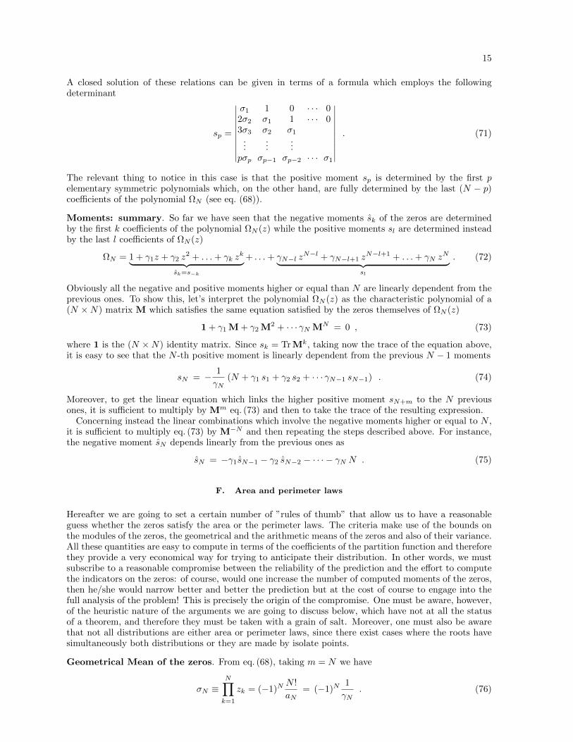
FIG. 5: a) Distribution of zeros of the partition function whose coefficients γk go as 1/k5. b) Distribution of zerosof the partition function whose coefficients γk go as k3. Notice that in both cases, all zeros, apart few, are placedalong a circle, i.e. they satisfy the perimeter law.
namely all of them belong to the class A. Therefore we expect that the polynomials of this class willsatisfy the perimeter law, apart eventually few zeros displaced somewhere else. Few experiments, inaddition to the one shown in Figure 4, are reported in Figure 5, and indeed they show that the zeros ofthese polynomials satisfy the perimeter law.
Case B. This case concerns with the values
| zgeom |' ξ , | zarith |= c , µ2 ' N (87)
A polynomial which has such values is
B(z) = zN +NzN−1 + 1 , (88)
(plus all other lower coefficients which however scale with lower powers in N) since
〈z〉geom = (1)1/N = 1 ,
〈z〉arith = −1 , (89)
µ2 =1
N
(1− 1
N
)N2 → N .
Notice that, in general, to have a finite geometrical mean not all zeros can grow as N , the same is alsotrue in order to have a finite value for the arithmetic mean. However, to have a variance which growsas N it is enough that some of the zeros are far off from 〈z〉arith, order N . This is indeed the case forthe roots of the polynomial (88), where one of them is far away from the arithmetic mean, z∗ ∼ −N ,while all the others are essentially along a circle of radius 1 and center at 〈z〉arith = −1. Therefore forpolynomials of this class we expect that, apart few zeros, the others satisfy a perimeter law. Notice thatin this case a bound such as the Fujiwara bound, taken alone, is pretty loose since it states that all rootssatisfy |zi| < 2N , a condition which is indeed true but in this case only one root is order N .
Case C. This case concerns with the values
| zgeom |' ξ , | zarith | ∼ N , µ2 ' N (90)
A polynomial with these properties is given by
C(z) = (z −N)N2
(z − 1
N
)N2
(91)
19
Assume N to be an even number. This polynomials has N/2 zeros at z = N and N/2 zeros at z = 1/N .Therefore the geometrical mean is equal to 1 while the arithmetic mean is equal to zarith = (N + 1/N)/2and its variance µ2 = (N − 1/N)2. In this case we are in presence of a bunch concentration of zeros (inthis case placed at reciprocal positions) which essentially do not satisfy neither area or perimeter laws.
Case D. This case concerns with
| zgeom |' ξ , | zarith |= N , µ2 ' ε (92)
A corresponding polynomial with these features is given by
D(z) = 1 + (N4 −N3 +N) zN−2 + 2N zN−1 + 2zN (93)
plus lowest order coefficients which scale with lower powers in N . Such a polynomial, apart few of itszeros which have large modules (order N) so that their arithmetic average goes with N , has the restof the zeros with bounded modules. Since their spread is small, most probably we are in presence of aperimeter law. In the case of the polynomial (93), its bounded zeros are indeed all around a circle.
Case E. This case concerns with
| zgeom |' N , | zarith | ' c , µ2 ' ε (94)
A representative polynomial with these features is
E(z) = 1 +N(N + 1)
2N !zN−2 +
1
(N − 1)!zN−1 +
1
N !zN , (95)
In order to compute the various statistical quantities we need the Stirling formula for the factorial
N ! '√
2πN
(N
e
)N. (96)
The divergence with N of the geometrical mean implies that almost all zeros has a module which increaseswith N although their barycenter remains at a finite distance. The infinitesimal value of the varianceonce again suggests that we may be in presence of a perimeter law. As a matter of fact, almost all rootsof the polynomial (95), varying N , are along a circle of increasing radius.
Case F. This case concerns with
| zgeom |' N , | zarith | ' c , µ2 ' N (97)
This class may have as a significant representative a polynomial which employs the prime numbers Pk
F (z) = 1 + P1z +1
2!P2z
2 + · · · 1
N !PNz
N (98)
In order to compute the various statistical quantities, in addition to the Stirling formula for the factorial,we also need the approximate formula for the N -the prime PN
PN ' N logN . (99)
Therefore
|zgeom| =
(1
γN
)1/N
∼ N ,
zarith = − 1
N
γN−1
γN∼ −1 (100)
µ2 ∼ N
Applying either the Fujiwara or the Enestrom bound, one sees that the radius of the disc which includesall zeros increases linearly with N . All these behaviors suggest that the zeros of the polynomial (98)satisfy the area law, which is indeed the case, as shown in Figure 4.
20
Case G. This case concerns with
| zgeom |' N , | zarith | ' N , µ2 ' ε (101)
A polynomial with these features is given by
G(z) = (z −N)N . (102)
The zeros of this polynomial are obviously all at z∗ = N . Both their arithmetic and geometric means areequal to N and therefore diverge when N →∞, however their variance is identically zero. When we arein presence of these values of the indicators it is quite probable that the distribution of zero is sharplypeaked around a value z∗ that grows with N . Also in this case the zeros do not satisfy neither area orperimeter laws.
Case H. This case concerns with
| zgeom |' N , | zarith | ' N , µ2 ' N (103)
A representative polynomial may be
H(z) = (z −N)(z −N + 1)(z −N + 2) · · · (z − 2N) . (104)
The zeros of this polynomial are z = N,N + 1, . . . , 2N . Their arithmetic mean is zarith = 3(N + 1)/2,its geometrical mean goes as zgeom ∼ N and its variance goes as µ2 ∼ N2/12. The geometrical shapeof these zeros consists of a cluster of N isolated zeros, all of order N , which move away from the originenlarging their spreading. This kink of zeros do not satisfy neither area nor perimeter law but are ratherdiscrete isolated points which move at z =∞ by increasing N .
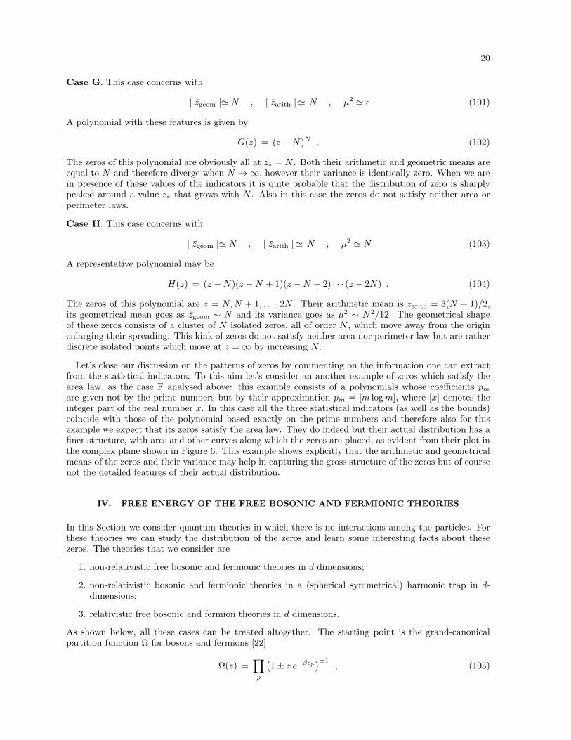
Let’s close our discussion on the patterns of zeros by commenting on the information one can extractfrom the statistical indicators. To this aim let’s consider an another example of zeros which satisfy thearea law, as the case F analysed above: this example consists of a polynomials whose coefficients pmare given not by the prime numbers but by their approximation pm = [m logm], where [x] denotes theinteger part of the real number x. In this case all the three statistical indicators (as well as the bounds)coincide with those of the polynomial based exactly on the prime numbers and therefore also for thisexample we expect that its zeros satisfy the area law. They do indeed but their actual distribution has afiner structure, with arcs and other curves along which the zeros are placed, as evident from their plot inthe complex plane shown in Figure 6. This example shows explicitly that the arithmetic and geometricalmeans of the zeros and their variance may help in capturing the gross structure of the zeros but of coursenot the detailed features of their actual distribution.
IV. FREE ENERGY OF THE FREE BOSONIC AND FERMIONIC THEORIES
In this Section we consider quantum theories in which there is no interactions among the particles. Forthese theories we can study the distribution of the zeros and learn some interesting facts about thesezeros. The theories that we consider are
1. non-relativistic free bosonic and fermionic theories in d dimensions;
2. non-relativistic bosonic and fermionic theories in a (spherical symmetrical) harmonic trap in d-dimensions;
3. relativistic free bosonic and fermion theories in d dimensions.
As shown below, all these cases can be treated altogether. The starting point is the grand-canonicalpartition function Ω for bosons and fermions [22]
Ω(z) =∏p
(1± z e−βεp
)±1, (105)
21
FIG. 6: An example of area law: distribution of zeros of the partition function where the coefficients are given byan = [n logn].
where + refers to fermion and − to boson, with the infinite product extended to all values p of themomentum which parameterises the energies of the excitation. Taking the logarithm of both sides weend up in
log Ω(z) = ±∑p
log(1± z e−βεp
)≡ F±(z, β) , (106)
where
F±(z, β) = ±∫dε g(ε) log
(1± z e−βε
). (107)
This universal way to express the free energy simply employs the density of states g(ε) of each system,whose definition is
g(ε) =
∫dr dp
(2π~)dδ(ε−H(r, p)) . (108)
We report hereafter the expression of the various densities of states (got by a straightforward calculation)and the expression of the relative free-energies for the various cases enumerated above.
1. Non-relativistic free bosonic and fermionic theories in d dimensions. Both these theorieshave the Hamiltonian
H =p2
2m, (109)
and their density of states is given by
gnr(ε) = V( m
2π~2
) d2 1
Γ(d2
) ε d2−1 . (110)
Substituting this expression in eq. (107) and expanding the logarithm for |z| < 1, we have
F±(z, β) =
∞∑k=1
∞∫0
dεg(ε)(∓1)k+1 zk
ke−kβε
=V
λdTf±(z; d) , (111)

22
where λT is the thermal wave-length
λT =
(2π~2
mkT
)1/2
, (112)
while the functions f±(z; d) depend upon only z and the dimensionality d, but not from the tem-perature T
f±(z; d) =
∞∑k=1
(∓1)k+1 zk
kd2 +1
. (113)
These functions can be expressed in terms of poly-logarithmic functions, defined by
Ls(z) =
∞∑k=1
zn
ns. (114)
More precisely, for the boson, we have
f−(z; d) = L d2 +1(z) , (115)
while for the fermion
f+(z; d) = −L d2 +1(−z) . (116)
2. Non-relativistic bosonic and fermion theories in a (spherical symmetrical) harmonictrap in d-dimensions.The Hamiltonian in this case is given by
H =p2
2m+
1
2mω2r2 , (117)
and the density of states is
gh(ε) =
(1
~ω
)d1
Γ (d)εd−1 . (118)
Notice that, apart from the prefactors, the density of states for the harmonic trap in d-dimensionis the same of the one of the free theories but in a dimension twice as large! Therefore, repeatingthe same computations as before, the expression of the free energies is
F±(z, β) =
(1
~ω
)df±(z; 2d) . (119)
3. Relativistic free bosonic and fermionic theories in d dimensions. The Hamiltonian of thesecases is
H =√p2 +m2 , (120)
and for the density of states we have
gr(ε) = 2V
(1
4π~2
) d2
ε(ε2 −m2)
) d2−1
. (121)
Repeating the same steps as before, we end up in the following expression of the free energies
F±(z, β) =V
λdT
√2mβ
πH±(z; d;β) , (122)
where
H±(z; d;β) =
∞∑n=1
(∓1)n+1
nd+12
K d+12
(nβm)zn , (123)
and Kν(z) is the modified Bessel function. In these relativistic cases the dependence on the tem-perature T no longer factorises as in the non-relativistic cases, but also enters explicitly the clustercoefficients through the Bessel function. These distributions correspond to free bosonic (− sub-script) and fermionic fields (+ subscript). In particular, for d = 1 the fermionic distribution isrelevant for the two-dimensional classical Ising model, regarded as a one-dimensional quantummodel of free Majorana fermions (see, for instance [16, 19, 20, 43, 44]).
23
V. DISTRIBUTION OF THE ZEROS FOR NON-RELATIVISTIC FREE THEORIES
In this Section we study the distribution of the zeros relative to the non-relativistic free theories. Sur-prisingly enough, there are I two alternative ways to address the problem that end up in two differentdistributions of the zeros. We denote the first method as Truncated Series Approach (TSA) while thesecond method as Infinite Product Approach (IPA). With the TSA, we will get an expression F1(z) of thefree energy of the systems which is valid in the disk |z| < 1 while, with the IPA, we will get instead anexpression F2(z) which extends to the entire complex plane, providing in particular the analytic contin-uation of F1(z) outside its disk of convergence. It is important to notice, though, that both distributionsof zeros share the same value of all the moments of the zeros. Let’s discuss these two methods in moredetail.
A. Truncated Series Approach
As shown in Section IV, there is a closed expression for the free energies F±(z, β) for the the non-relativistic free theories of bosons and fermions, see eq. (111). However, to determine the Yang-Lee zeros
we need to consider the zeros of the partition function itself, alias of a sequence of polynomials Ω(N)± (z, β)
in the limit N → ∞. This sequence of polynomials can be constructed by truncating the series relativeto F±(z, β) up to a given order N and then expanding the exponential exactly up to that order. In moredetail:
1. Let’s define the truncated expression of the free energies up to the order N as
F(N)± (z, β) ≡ V
λdT
N∑k=1
(∓1)k+1 zk
kd2 +1
. (124)
2. Let’s also define
Ω(N)± (z, β) ≡ eF
(N)± (z,β) , (125)
where Ω(N)± (x, β) is given by the Taylor series
Ω(N)± (x, β) ≡
N∑k=0
pkk!zk =
N∑k=0
zk
k!
dkΩ(N)±
dzk(0, β) , (126)
truncated at the order N . With the coefficients of the truncated polynomial Ω(N)± (x, β) determined as in
eq. (126), it is easy to see (compare with Section III) that – by construction – the negative moments ofthe zeros of this polynomial coincide exactly with those given in eq. (56)
sk = − V
λdT(∓1)k+1 1
kd2
. (127)
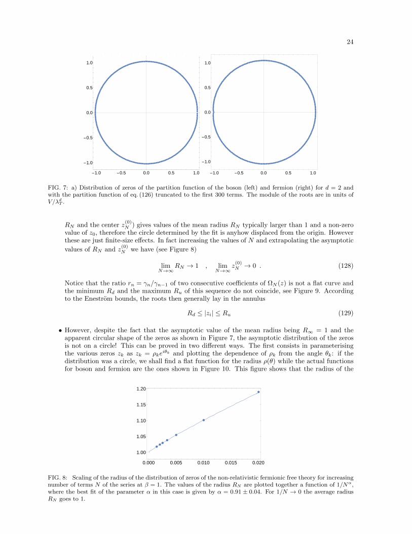
Let’s underline that in eq. (126) the coefficients pk relative to the bosonic case are all positive, while thoseof the fermionic case have alternating sign. In order to have always a positive and increasing value ofF (z) by increasing z, in the case of fermions it is convenient to always truncate at an even power of N .Let’s observe, moreover, that in all the expressions given above of the free energy the dependence uponthe volume V is always factorised. So, it is convenient to divide by V and consider the intensive part ofall quantities. Equivalently we can just work putting V = 1, which is what we have done in the rest ofthe paper for the distributions of the zeros associated to the actual partition functions. The numericaldetermination of the zeros of the polynomials (126) are shown in Figure 7, where the module of the rootsare expressed in unit of V/λdT .
There are many interesting features of the distribution of these zeros:
• for a finite value of N , the zeros are placed on a curve which looks to be a circle but as a matter offact is not! A fit of their location with a circle (i.e. with fit parameters given by the mean radius
24
-1.0 -0.5 0.0 0.5 1.0
-1.0
-0.5
0.0
0.5
1.0
-1.0 -0.5 0.0 0.5 1.0
-1.0
-0.5
0.0
0.5
1.0
FIG. 7: a) Distribution of zeros of the partition function of the boson (left) and fermion (right) for d = 2 andwith the partition function of eq. (126) truncated to the first 300 terms. The module of the roots are in units ofV/λdT .
RN and the center z(0)N ) gives values of the mean radius RN typically larger than 1 and a non-zero
value of z0, therefore the circle determined by the fit is anyhow displaced from the origin. Howeverthese are just finite-size effects. In fact increasing the values of N and extrapolating the asymptotic
values of RN and z(0)N we have (see Figure 8)
limN→∞
RN → 1 , limN→∞
z(0)N → 0 . (128)
Notice that the ratio rn = γn/γn−1 of two consecutive coefficients of ΩN (z) is not a flat curve andthe minimum Rd and the maximum Ru of this sequence do not coincide, see Figure 9. Accordingto the Enestrom bounds, the roots then generally lay in the annulus
Rd ≤ |zi| ≤ Ru (129)
• However, despite the fact that the asymptotic value of the mean radius being R∞ = 1 and theapparent circular shape of the zeros as shown in Figure 7, the asymptotic distribution of the zerosis not on a circle! This can be proved in two different ways. The first consists in parameterisingthe various zeros zk as zk = ρke
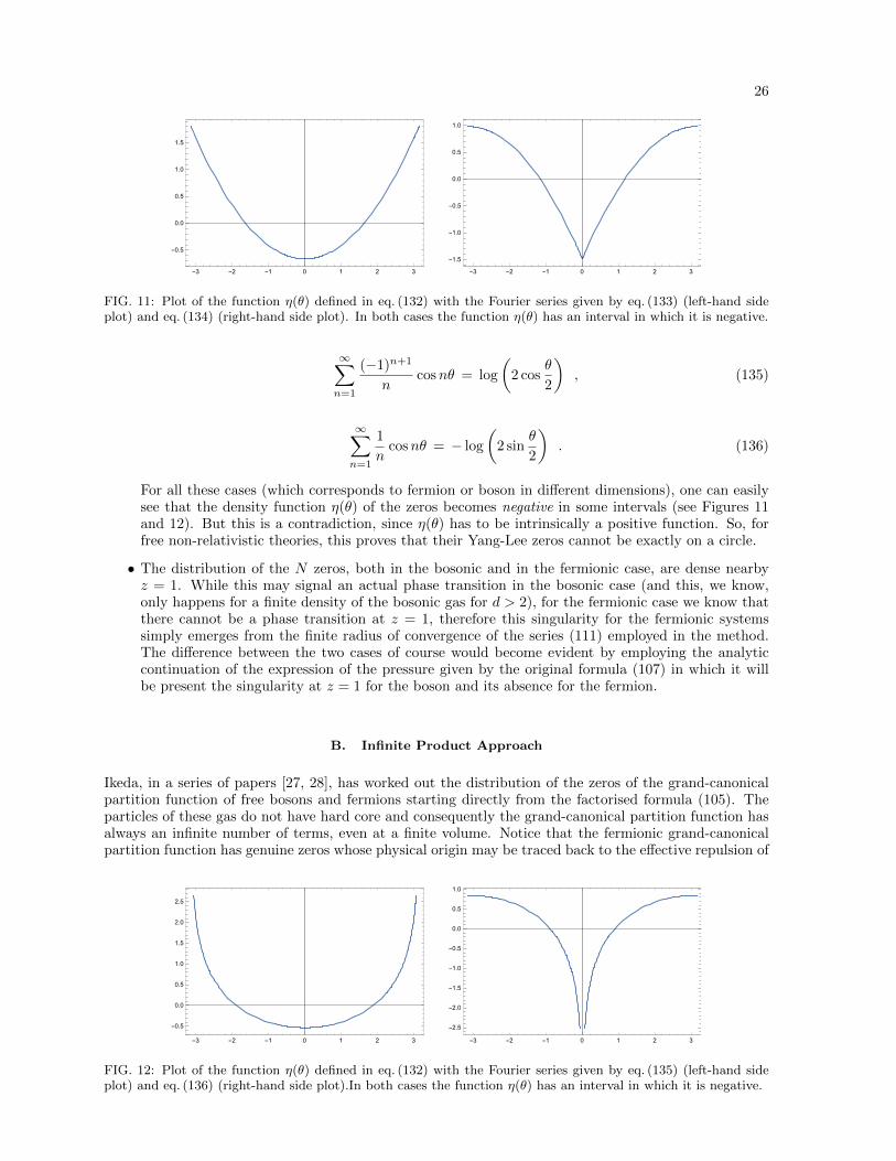
iθk and plotting the dependence of ρk from the angle θk: if thedistribution was a circle, we shall find a flat function for the radius ρ(θ) while the actual functionsfor boson and fermion are the ones shown in Figure 10. This figure shows that the radius of the
0.000 0.005 0.010 0.015 0.020
1.00
1.05
1.10
1.15
1.20
FIG. 8: Scaling of the radius of the distribution of zeros of the non-relativistic fermionic free theory for increasingnumber of terms N of the series at β = 1. The values of the radius RN are plotted together a function of 1/Nα,where the best fit of the parameter α in this case is given by α = 0.91 ± 0.04. For 1/N → 0 the average radiusRN goes to 1.
25
0 100 200 300 400 500
1.00
1.01
1.02
1.03
1.04
1.05
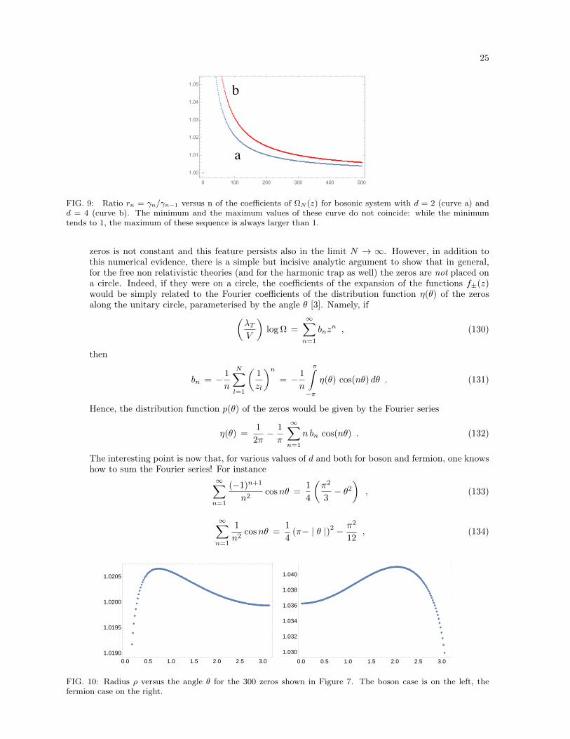
FIG. 9: Ratio rn = γn/γn−1 versus n of the coefficients of ΩN (z) for bosonic system with d = 2 (curve a) andd = 4 (curve b). The minimum and the maximum values of these curve do not coincide: while the minimumtends to 1, the maximum of these sequence is always larger than 1.
zeros is not constant and this feature persists also in the limit N → ∞. However, in addition tothis numerical evidence, there is a simple but incisive analytic argument to show that in general,for the free non relativistic theories (and for the harmonic trap as well) the zeros are not placed ona circle. Indeed, if they were on a circle, the coefficients of the expansion of the functions f±(z)would be simply related to the Fourier coefficients of the distribution function η(θ) of the zerosalong the unitary circle, parameterised by the angle θ [3]. Namely, if(
λTV
)log Ω =
∞∑n=1
bnzn , (130)
then
bn = − 1
n
N∑l=1
(1
zl
)n= − 1
n
π∫−π
η(θ) cos(nθ) dθ . (131)
Hence, the distribution function p(θ) of the zeros would be given by the Fourier series
η(θ) =1
2π− 1
π
∞∑n=1
n bn cos(nθ) . (132)
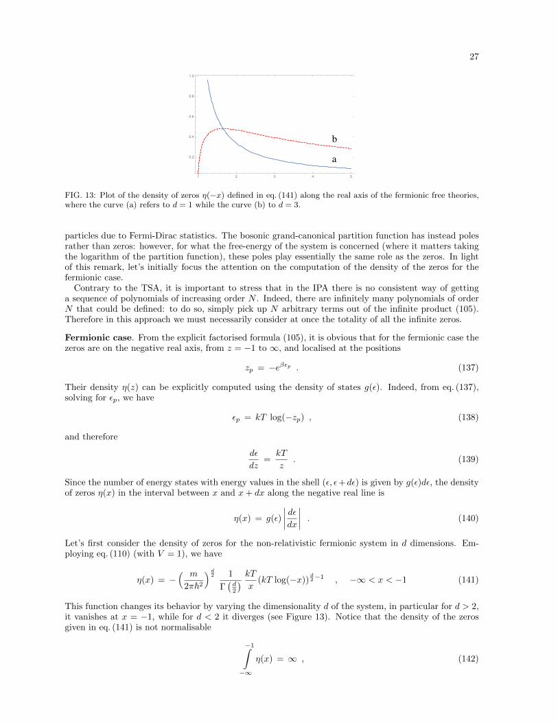
The interesting point is now that, for various values of d and both for boson and fermion, one knowshow to sum the Fourier series! For instance
∞∑n=1
(−1)n+1
n2cosnθ =
1
4
(π2
3− θ2
), (133)
∞∑n=1
1
n2cosnθ =
1
4(π− | θ |)2 − π2
12, (134)
0.0 0.5 1.0 1.5 2.0 2.5 3.0
1.0190
1.0195
1.0200
1.0205
0.0 0.5 1.0 1.5 2.0 2.5 3.0
1.030
1.032
1.034
1.036
1.038
1.040
FIG. 10: Radius ρ versus the angle θ for the 300 zeros shown in Figure 7. The boson case is on the left, thefermion case on the right.
26
FIG. 11: Plot of the function η(θ) defined in eq. (132) with the Fourier series given by eq. (133) (left-hand sideplot) and eq. (134) (right-hand side plot). In both cases the function η(θ) has an interval in which it is negative.
∞∑n=1
(−1)n+1
ncosnθ = log
(2 cos
θ
2
), (135)
∞∑n=1
1
ncosnθ = − log
(2 sin
θ
2
). (136)
For all these cases (which corresponds to fermion or boson in different dimensions), one can easilysee that the density function η(θ) of the zeros becomes negative in some intervals (see Figures 11and 12). But this is a contradiction, since η(θ) has to be intrinsically a positive function. So, forfree non-relativistic theories, this proves that their Yang-Lee zeros cannot be exactly on a circle.
• The distribution of the N zeros, both in the bosonic and in the fermionic case, are dense nearbyz = 1. While this may signal an actual phase transition in the bosonic case (and this, we know,only happens for a finite density of the bosonic gas for d > 2), for the fermionic case we know thatthere cannot be a phase transition at z = 1, therefore this singularity for the fermionic systemssimply emerges from the finite radius of convergence of the series (111) employed in the method.The difference between the two cases of course would become evident by employing the analyticcontinuation of the expression of the pressure given by the original formula (107) in which it willbe present the singularity at z = 1 for the boson and its absence for the fermion.
B. Infinite Product Approach
Ikeda, in a series of papers [27, 28], has worked out the distribution of the zeros of the grand-canonicalpartition function of free bosons and fermions starting directly from the factorised formula (105). Theparticles of these gas do not have hard core and consequently the grand-canonical partition function hasalways an infinite number of terms, even at a finite volume. Notice that the fermionic grand-canonicalpartition function has genuine zeros whose physical origin may be traced back to the effective repulsion of
FIG. 12: Plot of the function η(θ) defined in eq. (132) with the Fourier series given by eq. (135) (left-hand sideplot) and eq. (136) (right-hand side plot).In both cases the function η(θ) has an interval in which it is negative.
27
1 2 3 4 5
0.2
0.4
0.6
0.8
1.0
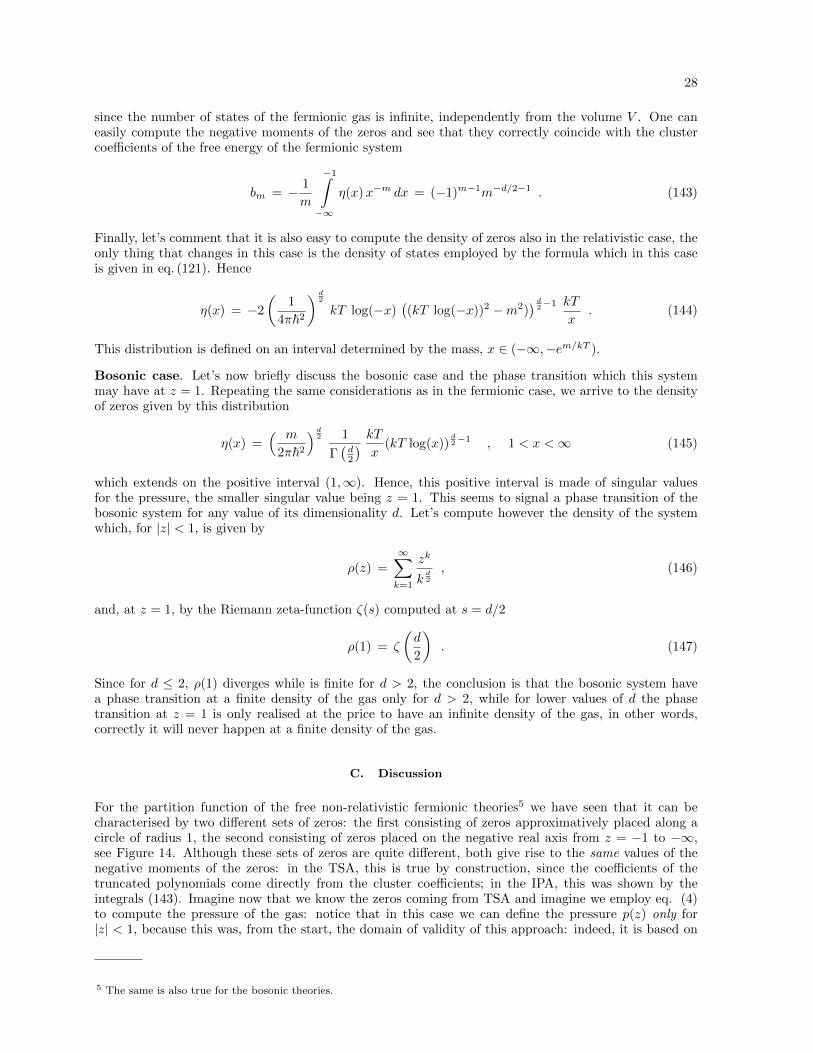
FIG. 13: Plot of the density of zeros η(−x) defined in eq. (141) along the real axis of the fermionic free theories,where the curve (a) refers to d = 1 while the curve (b) to d = 3.
particles due to Fermi-Dirac statistics. The bosonic grand-canonical partition function has instead polesrather than zeros: however, for what the free-energy of the system is concerned (where it matters takingthe logarithm of the partition function), these poles play essentially the same role as the zeros. In lightof this remark, let’s initially focus the attention on the computation of the density of the zeros for thefermionic case.
Contrary to the TSA, it is important to stress that in the IPA there is no consistent way of gettinga sequence of polynomials of increasing order N . Indeed, there are infinitely many polynomials of orderN that could be defined: to do so, simply pick up N arbitrary terms out of the infinite product (105).Therefore in this approach we must necessarily consider at once the totality of all the infinite zeros.
Fermionic case. From the explicit factorised formula (105), it is obvious that for the fermionic case thezeros are on the negative real axis, from z = −1 to ∞, and localised at the positions
zp = −eβεp . (137)
Their density η(z) can be explicitly computed using the density of states g(ε). Indeed, from eq. (137),solving for εp, we have
εp = kT log(−zp) , (138)
and therefore
dε
dz=
kT
z. (139)
Since the number of energy states with energy values in the shell (ε, ε+dε) is given by g(ε)dε, the densityof zeros η(x) in the interval between x and x+ dx along the negative real line is
η(x) = g(ε)
∣∣∣∣ dεdx∣∣∣∣ . (140)
Let’s first consider the density of zeros for the non-relativistic fermionic system in d dimensions. Em-ploying eq. (110) (with V = 1), we have
η(x) = −( m
2π~2
) d2 1
Γ(d2
) kTx
(kT log(−x))d2−1 , −∞ < x < −1 (141)
This function changes its behavior by varying the dimensionality d of the system, in particular for d > 2,it vanishes at x = −1, while for d < 2 it diverges (see Figure 13). Notice that the density of the zerosgiven in eq. (141) is not normalisable
−1∫−∞
η(x) = ∞ , (142)
28
since the number of states of the fermionic gas is infinite, independently from the volume V . One caneasily compute the negative moments of the zeros and see that they correctly coincide with the clustercoefficients of the free energy of the fermionic system
bm = − 1
m
−1∫−∞
η(x)x−m dx = (−1)m−1m−d/2−1 . (143)
Finally, let’s comment that it is also easy to compute the density of zeros also in the relativistic case, theonly thing that changes in this case is the density of states employed by the formula which in this caseis given in eq. (121). Hence
η(x) = −2
(1
4π~2
) d2
kT log(−x)((kT log(−x))2 −m2)
) d2−1 kT
x. (144)
This distribution is defined on an interval determined by the mass, x ∈ (−∞,−em/kT ).
Bosonic case. Let’s now briefly discuss the bosonic case and the phase transition which this systemmay have at z = 1. Repeating the same considerations as in the fermionic case, we arrive to the densityof zeros given by this distribution
η(x) =( m
2π~2
) d2 1
Γ(d2
) kTx
(kT log(x))d2−1 , 1 < x <∞ (145)
which extends on the positive interval (1,∞). Hence, this positive interval is made of singular valuesfor the pressure, the smaller singular value being z = 1. This seems to signal a phase transition of thebosonic system for any value of its dimensionality d. Let’s compute however the density of the systemwhich, for |z| < 1, is given by
ρ(z) =
∞∑k=1
zk
kd2
, (146)
and, at z = 1, by the Riemann zeta-function ζ(s) computed at s = d/2
ρ(1) = ζ
(d
2
). (147)
Since for d ≤ 2, ρ(1) diverges while is finite for d > 2, the conclusion is that the bosonic system havea phase transition at a finite density of the gas only for d > 2, while for lower values of d the phasetransition at z = 1 is only realised at the price to have an infinite density of the gas, in other words,correctly it will never happen at a finite density of the gas.
C. Discussion
For the partition function of the free non-relativistic fermionic theories5 we have seen that it can becharacterised by two different sets of zeros: the first consisting of zeros approximatively placed along acircle of radius 1, the second consisting of zeros placed on the negative real axis from z = −1 to −∞,see Figure 14. Although these sets of zeros are quite different, both give rise to the same values of thenegative moments of the zeros: in the TSA, this is true by construction, since the coefficients of thetruncated polynomials come directly from the cluster coefficients; in the IPA, this was shown by theintegrals (143). Imagine now that we know the zeros coming from TSA and imagine we employ eq. (4)to compute the pressure of the gas: notice that in this case we can define the pressure p(z) only for|z| < 1, because this was, from the start, the domain of validity of this approach: indeed, it is based on
5 The same is also true for the bosonic theories.
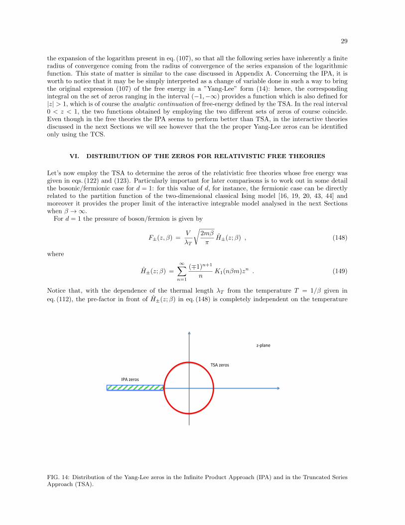
29
the expansion of the logarithm present in eq. (107), so that all the following series have inherently a finiteradius of convergence coming from the radius of convergence of the series expansion of the logarithmicfunction. This state of matter is similar to the case discussed in Appendix A. Concerning the IPA, it isworth to notice that it may be be simply interpreted as a change of variable done in such a way to bringthe original expression (107) of the free energy in a ”Yang-Lee” form (14): hence, the correspondingintegral on the set of zeros ranging in the interval (−1,−∞) provides a function which is also defined for|z| > 1, which is of course the analytic continuation of free-energy defined by the TSA. In the real interval0 < z < 1, the two functions obtained by employing the two different sets of zeros of course coincide.Even though in the free theories the IPA seems to perform better than TSA, in the interactive theoriesdiscussed in the next Sections we will see however that the the proper Yang-Lee zeros can be identifiedonly using the TCS.
VI. DISTRIBUTION OF THE ZEROS FOR RELATIVISTIC FREE THEORIES
Let’s now employ the TSA to determine the zeros of the relativistic free theories whose free energy wasgiven in eqs. (122) and (123). Particularly important for later comparisons is to work out in some detailthe bosonic/fermionic case for d = 1: for this value of d, for instance, the fermionic case can be directlyrelated to the partition function of the two-dimensional classical Ising model [16, 19, 20, 43, 44] andmoreover it provides the proper limit of the interactive integrable model analysed in the next Sectionswhen β →∞.
For d = 1 the pressure of boson/fermion is given by
F±(z, β) =V
λT
√2mβ
πH±(z;β) , (148)
where
H±(z;β) =
∞∑n=1
(∓1)n+1
nK1(nβm)zn . (149)
Notice that, with the dependence of the thermal length λT from the temperature T = 1/β given in
eq. (112), the pre-factor in front of H±(z;β) in eq. (148) is completely independent on the temperature
z-‐plane
IPA zeros
TSA zeros
FIG. 14: Distribution of the Yang-Lee zeros in the Infinite Product Approach (IPA) and in the Truncated SeriesApproach (TSA).
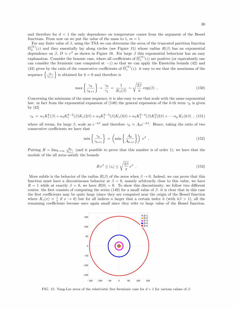
30
and therefore for d = 1 the only dependence on temperature comes from the argument of the Besselfunctions. From now on we put the value of the mass to 1, m = 1.
For any finite value of β, using the TSA we can determine the zeros of the truncated partition function
Ω(N)± (z) and they essentially lay along circles (see Figure 15) whose radius R(β) has an exponential
dependence on β, D ' eβ as shown in Figure 16. For large β this exponential behaviour has an easy
explanation. Consider the bosonic case, where all coefficients of Ω(N)+ (z) are positive (or equivalently one
can consider the fermionic case computed at −z) so that we can apply the Enestrom bounds (42) and
(43) given by the ratio of the consecutive coefficients of Ω(N)+ (z): it easy to see that the maximum of the
sequence
γkγk+1
is obtained for k = 0 and therefore is
max
γkγk+1
=
γ0
γ1=
1
K1(β)∼√
2β
πexp(β) , (150)
Concerning the minimum of the same sequence, it is also easy to see that scale with the same exponentiallaw: in fact from the exponential expansion of (148) the general expression of the k-th term γk is givenby [42]
γk = α1Kk1 (β) +α2K
k−21 (β)K1(2β) +α3K
k−31 (β)K1(3β) +α3K
k−41 (β)K2
1 (2β) + · · ·αpK1(kβ) , (151)
where all terms, for large β, scale as e−kβ and therefore γk ' Ake−kβ . Hence, taking the ratio of two
consecutive coefficients we have that
min
γkγk+1
=
(min
AkAk+1
)eβ . (152)
Putting B = limk→∞AkAk+1
(and it possible to prove that this number is of order 1), we have that the
module of the all zeros satisfy the bounds
B eβ ≤ |zi| ≤√
2β
πeβ . (153)
More subtle is the behavior of the radius R(β) of the zeros when β → 0. Indeed, we can prove that thisfunction must have a discontinouos behavior at β = 0, namely arbitrarily close to this value, we haveR = 1 while at exactly β = 0, we have R(0) = 0. To show this discontinuity, we follow two differentroutes: the first consists of computing the series (149) for a small value of β: it is clear that in this casethe first coefficients may be quite large (since they are computed near the origin of the Bessel functionwhere K1(x) ' 1
x if x → 0) but for all indices n larger that a certain index n (with nβ > 1), all theremaining coefficients become once again small since they refer to large value of the Bessel function.
- 150 - 100 - 50 0 50 100 150
- 150
- 100
- 50
0
50
100
150 β=1 β=2 β=3 β=4 β=5
FIG. 15: Yang-Lee zeros of the relativistic free fermionic case for d = 1 for various values of β.
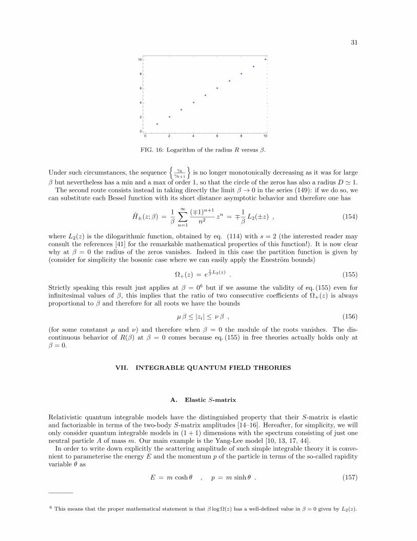
31
FIG. 16: Logarithm of the radius R versus β.
Under such circumstances, the sequence
γkγk+1
is no longer monotonically decreasing as it was for large
β but nevertheless has a min and a max of order 1, so that the circle of the zeros has also a radius D ' 1.The second route consists instead in taking directly the limit β → 0 in the series (149): if we do so, we
can substitute each Bessel function with its short distance asymptotic behavior and therefore one has
H±(z;β) =1
β
∞∑n=1
(∓1)n+1
n2zn = ∓ 1
βL2(±z) , (154)
where L2(z) is the dilogarithmic function, obtained by eq. (114) with s = 2 (the interested reader mayconsult the references [41] for the remarkable mathematical properties of this function!). It is now clearwhy at β = 0 the radius of the zeros vanishes. Indeed in this case the partition function is given by(consider for simplicity the bosonic case where we can easily apply the Enestrom bounds)
Ω+(z) = e1βL2(z) . (155)
Strictly speaking this result just applies at β = 06 but if we assume the validity of eq. (155) even forinfinitesimal values of β, this implies that the ratio of two consecutive coefficients of Ω+(z) is alwaysproportional to β and therefore for all roots we have the bounds
µβ ≤ |zi| ≤ ν β , (156)
(for some constanst µ and ν) and therefore when β = 0 the module of the roots vanishes. The dis-continuous behavior of R(β) at β = 0 comes because eq. (155) in free theories actually holds only atβ = 0.
VII. INTEGRABLE QUANTUM FIELD THEORIES
A. Elastic S-matrix
Relativistic quantum integrable models have the distinguished property that their S-matrix is elasticand factorizable in terms of the two-body S-matrix amplitudes [14–16]. Hereafter, for simplicity, we willonly consider quantum integrable models in (1 + 1) dimensions with the spectrum consisting of just oneneutral particle A of mass m. Our main example is the Yang-Lee model [10, 13, 17, 44].
In order to write down explicitly the scattering amplitude of such simple integrable theory it is conve-nient to parameterise the energy E and the momentum p of the particle in terms of the so-called rapidityvariable θ as
E = m cosh θ , p = m sinh θ . (157)
6 This means that the proper mathematical statement is that β log Ω(z) has a well-defined value in β = 0 given by L2(z).
32
The two-body S-matrix amplitude is then defined by
|A(θ1)A(θ2)〉 = S(θ1 − θ2) |A(θ2)A(θ1)〉 . (158)
It depends on the difference of the rapidities θ ≡ θ1−θ2 and satisfies the unitarity and crossing equations[14–16]
S(θ)S(−θ) = 1 , (159)
S(θ) = S(iπ − θ) . (160)
As evident from eq. (158), the S-matrix also plays the role of braiding matrix, interchanging the rapiditiesof the two particles. Notice that the unitarity condition (159) forces the value of the S-matrix at θ = 0 tobe S(0) = ±1. Consistent models have been found only for S = −1 (see, for instance, [46]): models whoseS-matrix satisfies S(0) = −1 are called fermionic models because, looking at eq. (158), interchanging twoexcitations of equal rapidities, their wave-function changes sign. As discussed below, this property isimportant for the thermodynamics of the integrable models. Let us notice that for such simple quantumintegrable systems the S-matrix is a pure phase
S(θ) = eiδ(θ) , (161)
where δ(θ) is the phase shift. For later use it is convenient to introduce the kernel ϕ(θ), given by thederivative of the phase shift
ϕ(θ) =dδ(θ)
dθ. (162)
B. Thermodynamic Bethe Ansatz
Al.B. Zamolodchikov [17] derived the basic equations which allows us to compute the free-energy of aquantum integrable model defined on a cylinder of width β and length L. The radius β of the cylinderis directly associated to the temperature T of the system through the relation β = 1/T while L is thevolume of the system. The formalism can be generalised to include also the chemical potential [19, 20]and the final equations read as follow: the pressure p(z) is expressed by
β p(z) =
∞∫−∞
dθ
2πcosh θ log
(1 + z e−ε(θ,z)
), (163)
where the function ε(θ, z) (called pseudo-energy) satisfies the non-linear integrable equation
ε(θ, z) = mβ cosh θ −∞∫−∞
dθ′
2πϕ(θ − θ′) log
(1 + z e−ε(θ
′,z)). (164)
Therefore the partition function of the system is given by
Ω(z) = exp
mL +∞∫−∞
cosh θ log(
1 + z e−ε(θ,z)) dθ
2π
. (165)
Notice that Ω(z) refers already to the thermodynamic limit where both L and the number of particlesN go to infinity with their ratio given by the density ρ(z) = z dΩ
dz at a fixed value of z. It is worthnoticing that the pressure has formally the same expression as in the free theories, the only difference isthat while in free theories the pseudo-energy ε(θ) coincides with the energy of the particle7 multiplied by
7 If the theory is free the S-matrix is a constant and therefore the kernel ϕ(θ) vanishes. Therefore, in this case, eq.(164)states that ε(θ) = mβ cosh θ
33
β, in an interactive integrable theory it satisfies instead the non-linear integral equation (164). Observethat the pseudo-energy ε(θ, z) of course also depends on β but we avoid to write this explicitly to keepthe notation simpler. The partition function (165) does not have a singularity for positive value of z, inagreement with the purely massive behavior of the theory and its fermionic nature.
In summary, for a a quantum integrable model, it is sufficient to know its S-matrix for computing itspartition function (165) at a finite temperature and a chemical potential through the equations (163)and (164). In the next Section we will study the zeros of this partition function for one of the simplestintegrable quantum field theories, the Yang-Lee model.
VIII. PARTITION FUNCTION OF THE YANG-LEE MODEL
In this Section, using the TSA described in Section V A, we are going to determine the distribution ofthe Yang-Lee zeros of the Yang-Lee model in (1+1) dimensions. To proceed, let’s briefly recall the exactS-matrix of this model.
A. S-matrix of the Yang-Lee model
An example of the S-matrix which satisfy all the requirements discussed above is
SY L(θ) =tanh 1
2
(θ + 2πi
3
)tanh 1
2
(θ − 2πi
3
) . (166)
In [10] it has been identified with the exact scattering amplitude of the massive theory that comes fromthe deformation of the non-unitarity conformal minimal model with central charge c = −22/5 [11] madeby its only relevant field φ of conformal dimension ∆ = −1/5. Apart being a fermionic S-matrix, theamplitude (166) has its own peculiarities: first of all, it has a pole at θ = 2πi
3 and another at θ = iπ3which correspond to the same particle A that appears as a bound state of itself both in the s and thet-channel. Secondly, the residue of the S-matrix at the pole in the s-channel has the ”wrong” sign withwhat usually expected in an hermitian theory. Generally, the residue in the s-channel pole at iu of anS-matrix is associated to the Feynamn diagram shown in Figure 17
S(θ) = ig2
θ − iu, (167)
and therefore it corresponds to the square of the on-shell three-point coupling constant g. Since thisquantity in an hermitian theory is real, the residue is positive. But in Yang-Lee model the couplingconstant is purely imaginary, as evident from its action (2) and therefore the residue of this theory at thes-channel pole θ = 2πi
3 is negative, as confirmed by its explicit computation
i g2 = i tan2π
3= −√
3 i . (168)
The action (2) is not hermitian but nevertheless CP invariant. The way to see this is to introduce theoperator CP which changes φ in −φ, under which A† = (CP )A (CP ). This relation ensures the realityof the spectrum but implies a modification in the completeness relation given by the multi-state sum, forthe Yang-Lee model given by ∑
N=0
(−1)N |N〉 〈N | = 1 . (169)
B. Solution of the Bethe Ansatz equations
The non-linear integral equation for the pseudo-energy of the Yang-Lee model is given by (we put themass m = 1)
ε(θ, z) = β cosh θ +
∞∫−∞
√3 cosh(θ)(
sinh2(θ) + 34
) ln(1 + ze−ε(θ′,z))
dθ′
2π. (170)
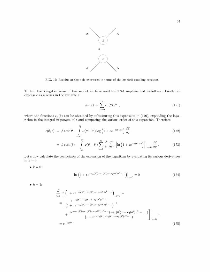
34
A A
AA
A
g
g
FIG. 17: Residue at the pole expressed in terms of the on-shell coupling constant.
To find the Yang-Lee zeros of this model we have used the TSA implemented as follows. Firstly weexpress ε as a series in the variable z
ε(θ, z) =
∞∑n=0
εn(θ) zn , (171)
where the functions εn(θ) can be obtained by substituting this expression in (170), expanding the loga-rithm in the integral in powers of z and comparing the various order of this expansion. Therefore
ε(θ, z) = β cosh θ −∞∫−∞
ϕ(θ − θ′) log(
1 + ze−ε(θ′,z)) dθ′
2π(172)
= β cosh(θ)−∞∫−∞
ϕ(θ − θ′)∞∑k=0
zk
k!
∂k
∂zk
[ln(
1 + ze−ε(θ′,z))]∣∣∣
z=0
dθ′
2π. (173)
Let’s now calculate the coefficients of the expansion of the logarithm by evaluating its various derivativesin z = 0:
• k = 0:
ln(
1 + ze−ε0(θ′)−ε1(θ′)z−ε2(θ′)z2−...)∣∣∣z=0
= 0 (174)
• k = 1:
∂
∂zln(
1 + ze−ε0(θ′)−ε1(θ′)z−ε2(θ′)z2−...)∣∣∣z=0
=
=
[e−ε0(θ′)−ε1(θ′)z−ε2(θ′)z2−...(
1 + ze−ε0(θ′)−ε1(θ′)z−ε2(θ′)z2−...) +
+ze−ε0(θ′)−ε1(θ′)z−ε2(θ′)z2−...(−ε1(θ′)z − ε2(θ′)z2 − . . .)(
1 + ze−ε0(θ′)−ε1(θ′)z−ε2(θ′)z2−...) ]∣∣∣∣∣
z=0
=
= e−ε0(θ′) (175)
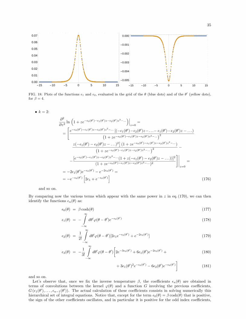
35
-15 -10 -5 0 5 10 150.00
0.01
0.02
0.03
0.04
0.05
0.06
0.07
-15 -10 -5 0 5 10 15
-0.005
-0.004
-0.003
-0.002
-0.001
0.000
FIG. 18: Plots of the functions ε1 and ε2, evaluated in the grid of the θ (blue dots) and of the θ′ (yellow dots),for β = 4.
• k = 2:
∂2
∂z2ln(
1 + ze−ε0(θ′)−ε1(θ′)z−ε2(θ′)z2−...)∣∣∣z=0
=
=
[e−ε0(θ′)−ε1(θ′)z−ε2(θ′)z2−... [(−ε1(θ′)−ε2(θ′)z−. . .− ε1(θ′)−ε2(θ′)z − . . .)(
1 + ze−ε0(θ′)−ε1(θ′)z−ε2(θ′)z2−...)2
z(−ε1(θ′)− ε2(θ′)z − . . .)2]
(1 + ze−ε0(θ′)−ε1(θ′)z−ε2(θ′)z2−...)(1 + ze−ε0(θ′)−ε1(θ′)z−ε2(θ′)z2−...
)2 −
− [e−ε0(θ′)−ε1(θ′)z−ε2(θ′)z2−...(1 + z(−ε1(θ′)− ε2(θ′)z − . . .))]2
(1 + ze−ε0(θ′)−ε1(θ′)z−ε2(θ′)z2−...)2
]∣∣∣∣∣z=0
=
= −2ε1(θ′)e−ε0(θ′) − e−2ε0(θ′) =
= −e−ε0(θ′)[2ε1 + e−ε0(θ′)
](176)
and so on.
By comparing now the various terms which appear with the same power in z in eq. (170), we can thenidentify the functions εn(θ) as:
ε0(θ) = β cosh(θ) (177)
ε1(θ) = −∞∫−∞
dθ′ϕ(θ − θ′)e−ε0(θ′) (178)
ε2(θ) =1
2!
∞∫−∞
dθ′ϕ(θ − θ′)[2ε1e−ε0(θ′) + e−2ε0(θ′)] (179)
ε3(θ) = − 1
3!
∞∫−∞
dθ′ϕ(θ − θ′)[2e−3ε0(θ′) + 6ε1(θ′)e−2ε0(θ′) + (180)
+ 3ε1(θ′)2e−ε0(θ′) − 6ε2(θ′)e−ε0(θ′)
](181)
and so on.Let’s observe that, once we fix the inverse temperature β, the coefficients εn(θ) are obtained in
terms of convolutions between the kernel ϕ(θ) and a function G involving the previous coefficients,G (ε1(θ′), . . . , εn−1(θ′)). The actual calculation of these coefficients consists in solving numerically thishierarchical set of integral equations. Notice that, except for the term ε0(θ) = β cosh(θ) that is positive,the sign of the other coefficients oscillates, and in particular it is positive for the odd index coefficients,
36
and negative for the even index ones. This will induce an expansion of the free-energy in terms of a seriesof alternating terms and ultimately a partition function with positive and negative coefficients, as in thecase of free fermionic theory.
C. Calculation of the free energy
We can now compute the pressure using the same method adopted for the pseudo-energy. In fact we canwrite it as an expansion:
p(β, z) ≡∑n
fn(β) zn (182)
with the coefficients fn(β) obtained by expanding the integrand of the eq. 163)
p(β, z) =1
β
∞∫−∞
dθ
2π
∑k
zk
k!
∂k
∂zk
[ln(1 + ze−ε(θ))
]∣∣∣z=0
(183)
The coefficients have the following expression:
f0(β) = 0 (184)
f1(β) =1
β
∞∫−∞
dθ
2πcosh(θ)e−ε0(θ) (185)
f2(β) = − 1
2!β
∞∫−∞
dθ
2πcosh(θ)[2ε1e
−ε0(θ′) + e−2ε0(θ′)] (186)
f3(β) =1
3!β
∞∫−∞
dθ
2πcosh(θ)
[2e−3ε0(θ′) + 6ε1(θ′)e−2ε0(θ′) + (187)
+ 3ε1(θ′)2e−ε0(θ′) − 6ε2(θ′)e−ε0(θ′)
](188)
and so on. Notice that also in this case we have alternating sign for the coefficients, but the negativeones are those with an even index.
D. Calculation of the zeros of the partition function
We can now determine the zeros of the partition function, written as polynomial in the fugacity z usingthe expansion:
Ω(z) = exp
[β∑i
fi(z) zi
]≡∑k
pkzk (189)
where:
pk =1
k!
∂k exp[β∑i fi(z, β)zi
]∂zk
∣∣∣∣∣z=0
(190)
We can verify that also in this case, as for the fermionic free theory, the coefficients of the expansion inz of the partition function, except for the zero order term, have alternating signs, in particular the evenindex coefficients are negative and the odd index coefficients are positive.

37
- 20 - 10 0 10 20
- 20
- 10
0
10
20 β=1 β=2 β=3 β=4 β=5
- 15 - 10 - 5 0 5 10 15
- 15
- 10
- 5
0
5
10
15 β=1 β=2 β=3 β=4 β=5
FIG. 19: a) Distribution of zeros of the partition function for fermionic Yang-Lee model for different values ofβ, obtained with the analytical calculations of the first 24 coefficients of the expansion; b) Distribution of zerosof the partition function for fermionic Yang-Lee model for different values of β, obtained with 500 coefficientsobtained by using their scaling law (191).
E. Results for finite β
Once we obtain the expression of the partition function as a polynomial in the fugacity z, we can studythe distribution of its zeros. For each value of β, we find that the zeros lay along an approximatecircumference, whose radius increases with β as shown in Fig. 19. As a matter of fact, given the enormousnumber of terms generated by the various series expansions described above, the analytic computationcan be handle only up to 24 terms. However, we have pushed further the order of the polynomial byusing a scaling law satisfied by the coefficients fn(β) in eq. (182)
fn(β)
fn−1(β)' 1
zc(β)
(1 +
α(β)− 1
n
), (191)
where both the parameters zc(β) and α(β) depends on β. This scaling law is shown in Figure 20 fora particular value of β. Using the scaling law (191) we study the zeros of polynomials up to order500. Increasing the order of the polynomial we observe that the average values of the radius of thecircle distribution of the zeros shows a convergence to final values which depend on β, as shown inFig. 21. Contrary to the free cases, for the interactive Yang-Lee model the radius R(β) of its zeros goescontinuously to zero when β → 0 with an overall law which a best fit of the data fixes to be
R(β) = eβ − 1 . (192)
We now show that we can easily predict the behavior of R(β) at β →∞ and at β → 0.
F. The β →∞ limit
In the limit β → ∞, the distribution of zeros of the partition function of the Yang-Lee model simplyreduces to that of the free fermionic theory. In fact, for large value of β, the pseudo-energy becomes theone of free theory ε(θ) ' β cosh θ and also its partition function
Ω(z) ' exp
L +∞∫−∞
cosh θ log(
1 + z e−β cosh θ)) dθ
2π
. (193)
The zeros of the Yang-Lee model in this limit thus coincide with those of the one-dimensional freefermionic model and therefore the radius R(β) of the zeros scales for β →∞ as R(β) ' eβ .
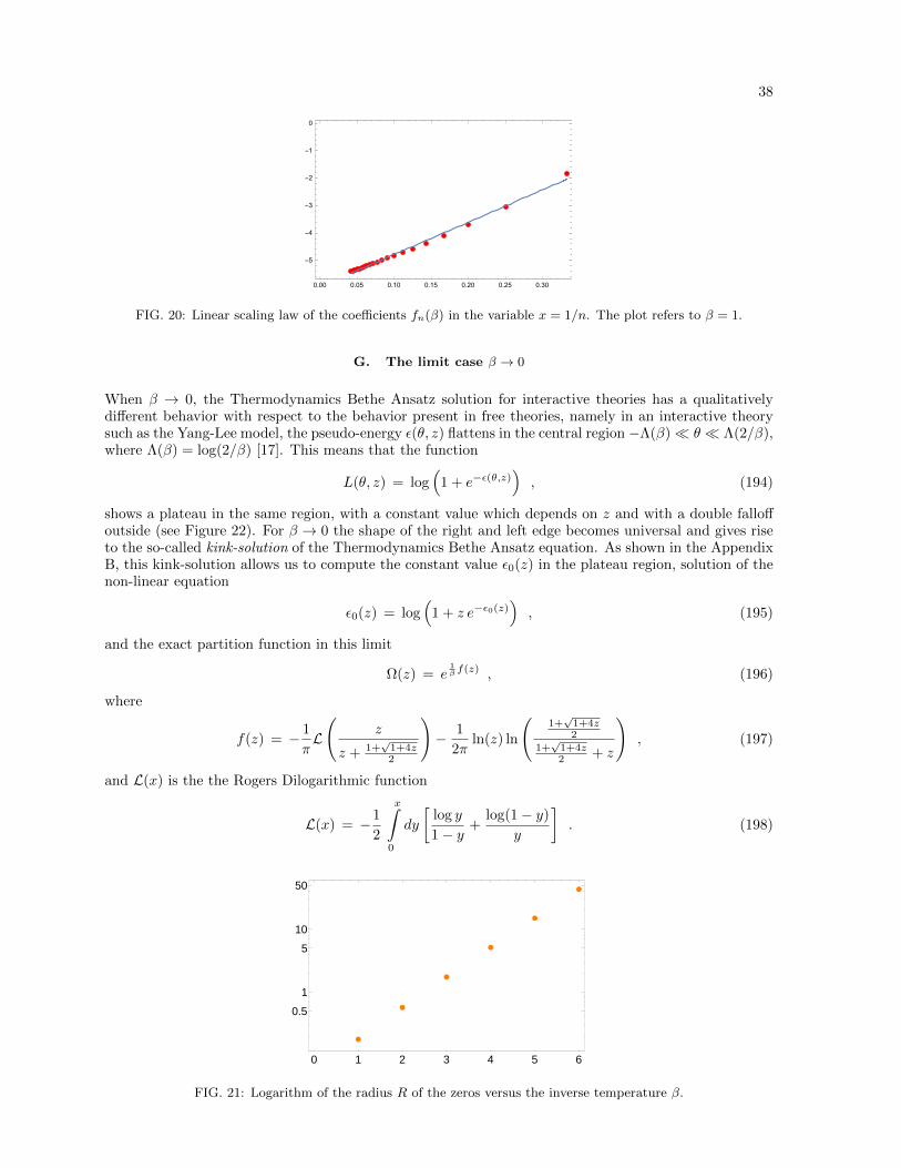
38
FIG. 20: Linear scaling law of the coefficients fn(β) in the variable x = 1/n. The plot refers to β = 1.
G. The limit case β → 0
When β → 0, the Thermodynamics Bethe Ansatz solution for interactive theories has a qualitativelydifferent behavior with respect to the behavior present in free theories, namely in an interactive theorysuch as the Yang-Lee model, the pseudo-energy ε(θ, z) flattens in the central region −Λ(β) θ Λ(2/β),where Λ(β) = log(2/β) [17]. This means that the function
L(θ, z) = log(
1 + e−ε(θ,z)), (194)
shows a plateau in the same region, with a constant value which depends on z and with a double falloffoutside (see Figure 22). For β → 0 the shape of the right and left edge becomes universal and gives riseto the so-called kink-solution of the Thermodynamics Bethe Ansatz equation. As shown in the AppendixB, this kink-solution allows us to compute the constant value ε0(z) in the plateau region, solution of thenon-linear equation
ε0(z) = log(
1 + z e−ε0(z)), (195)
and the exact partition function in this limit
Ω(z) = e1β f(z) , (196)
where
f(z) = − 1
πL
(z
z + 1+√
1+4z2
)− 1
2πln(z) ln
(1+√
1+4z2
1+√
1+4z2 + z
), (197)
and L(x) is the the Rogers Dilogarithmic function
L(x) = −1
2
x∫0
dy
[log y
1− y+
log(1− y)
y
]. (198)
0 1 2 3 4 5 6
0.5
1
5
10
50
FIG. 21: Logarithm of the radius R of the zeros versus the inverse temperature β.
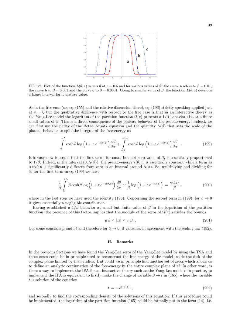
39
-15 -10 -5 0 5 10 15
0.0
0.1
0.2
0.3
0.4
0.5
FIG. 22: Plot of the function L(θ, z) versus θ at z = 0.5 and for various values of β: the curve a refers to β = 0.01,the curve b to β = 0.001 and the curve c to β = 0.0001. Going to smaller value of β, the function L(θ, z) developsa larger interval for it plateau value.
As in the free case (see eq. (155) and the relative discussion there), eq. (196) strictly speaking applied justat β = 0 but the qualitative difference with respect to the free case is that in an interactive theory asthe Yang-Lee model the logarithm of the partition function Ω(z) presents a 1/β behavior also at a finitesmall values of β! This is a direct consequence of the plateau behavior of the pseudo-energy: indeed, wecan first use the parity of the Bethe Ansatz equation and the quantity Λ(β) that sets the scale of theplateau behavior to split the integral of the free-energy as
+Λ∫0
cosh θ log(
1 + z e−ε(θ,z)) dθ
2π+
+∞∫−Λ
cosh θ log(
1 + z e−ε(θ,z)) dθ
2π. (199)
It is easy now to argue that the first term, for small but not zero value of β, is essentially proportionalto 1/β. Indeed, in the interval (0,Λ(β)), the pseudo-energy ε(θ, z) is essentially constant while a term asβ cosh θ is significantly different from zero in an interval around Λ(β). So, multiplying and dividing forβ, for the first term in eq. (199) we have
1
β
+Λ∫0
β cosh θ log(
1 + z e−ε(θ,z)) dθ
2π' 1
βlog(
1 + z e−ε0(z))
=ε0(z)
β, (200)
where in the last step we have used the identity (195). Concerning the second term in (199), for β → 0it gives essentially a negligible contribution.
Having established a 1/β behavior at small but finite value of β in the logarithm of the partitionfunction, the presence of this factor implies that the module of the zeros of Ω(z) satisfies the bounds
µ β ≤ |zi| ≤ ν β , (201)
(for some constans µ and ν) and therefore for β → 0, it vanishes, in agreement with the scaling law (192).
H. Remarks
In the previous Sections we have found the Yang-Lee zeros of the Yang-Lee model by using the TSA andthese zeros could be in principle used to reconstruct the free energy of the model inside the disk of thecomplex plane limited by their radius. But could we in principle find another set of zeros which allows usto define an analytic continuation of the free-energy in the entire complex plane of z? In other word, isthere a way to implement the IPA for an interactive theory such as the Yang-Lee model? In practise, toimplement the IPA is equivalent to firstly make the change of variable β → t in (165), where the variablet is solution of the equation
t = −eε(β,z) , (202)
and secondly to find the corresponding density of the solutions of this equation. If this procedure couldbe implemented, the logarithm of the partition function (165) could be formally put in the form (14), i.e.
40
an integral on the zeros of the theory. All these steps seem to follow closely the IPA implemented for thefree theories (see Section V B) but for interactive theories there is an important difference: the variable tthat solves eq.(202) depends itself on z! This implies that, in the interactive case, in order to implementthe IPA one is forced to introduce an infinite number of distributions of zeros, according to the values ofz for which we want to evaluate the free-energy. Although nothing wrong with this procedure, of courseits implementation is not particularly practical. This essentially seems to leave the TSA as the mostconvenient method to identify the Yang-Lee zeros in interacting integrable models.
IX. CONCLUSIONS
In this paper we have discussed the Yang-Lee zeros for a quantum integrable field theory particularlysimple, the Yang-Lee model. To compute such zeros, we have relied on the exact expression of thefree-energy of the model expressed by the Thermodynamics Bethe Ansatz equations based on the exactS-matrix of the theory. We have used in particular the so-called Truncated Series approach to define asequence of polynomials, each of them regarded as an approximation of the exact partition function ofthe model at a given order N in the fugacity z: increasing N , the zeros of these polynomials identify theYang-Lee zeros of the model. As a matter of fact, they are distributed around approximate circles whoseradius depends exponentially on the inverse temperature β. This feature may be also present in otherintegrable quantum field theories and it would be interesting to confirm or disprove this fact.
In addition to satisfy the curiosity to see, at least in one explicit example, where the Yang-Lee zerosare located for quantum integrable field theories, in our opinion there are other interesting questions thatcome out from our analysis and which deserve future attention. The most important one concerns thepossibility to invert the logic behind the theory of Yang-Lee zeros, namely to see whether it would bepossible to use the distributions of zeros for defining well defined statistical models and what propertiesthey would have. Is any distribution of zeros which leads to positive polynomials a good one? Forinstance, what is (if any) the statistical model behind the partition function (98) based on the primenumbers? Is it a local or non-local model? We denote such a kind of questions the inverse Yang-Leeproblem.
To make any progress in such a program, one shall be aware however of another important aspect:beside some very special cases, as for instance the one analysed in [30], the knowledge of the Yang-Leezeros alone is of course not enough to address other important properties of the model, as for instance,the computation of its correlation functions. In light of this remark, as a first important step forward,it would be extremely interesting to identify what is the minimum set of quantities (in addition to thedensity of the Yang-Lee zeros) which would allow – at least in principle – to successfully deal with theinverse Yang-Lee problem.
Acknowledgements
One of us (GM) is grateful to Don Zagier for very useful discussion and also acknowledges the BrazilianMinistry of Education (MEC) and the UFRN-FUNPEC for financial support during his visit to theInternational Institute of Physics in Natal, where this work was completed. GM also thanks AlvaroFerraz and other members of IIP for the warm hospitality.
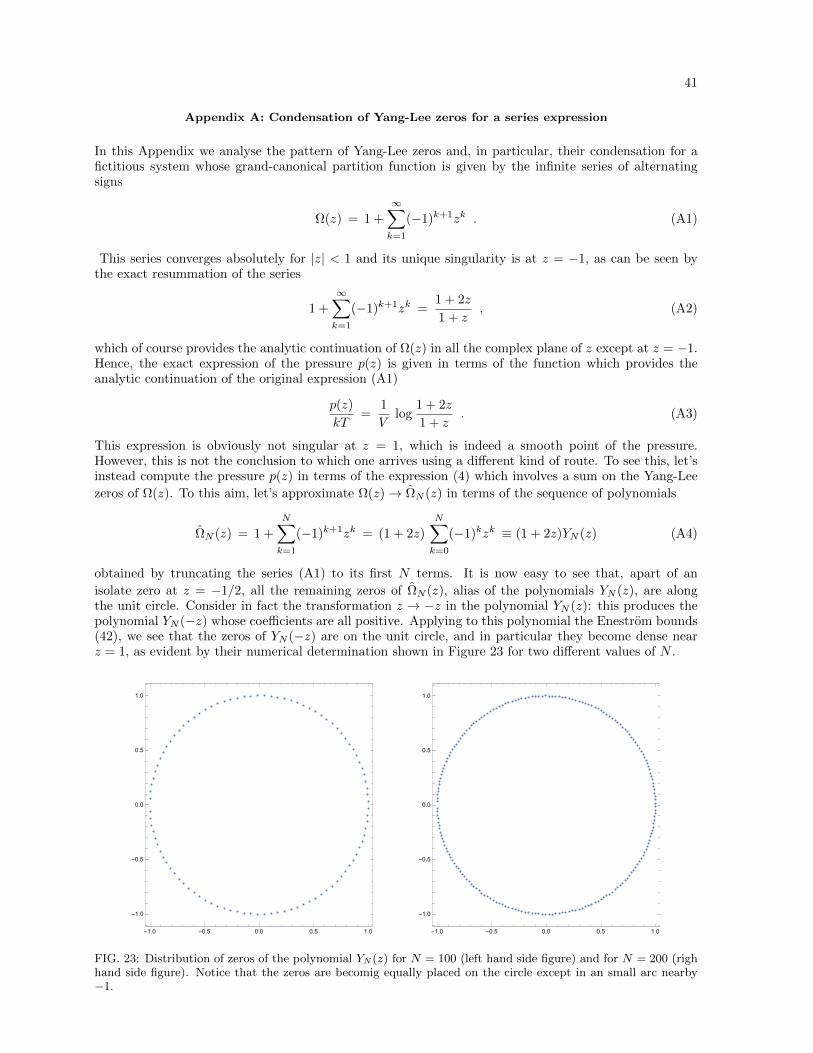
41
Appendix A: Condensation of Yang-Lee zeros for a series expression
In this Appendix we analyse the pattern of Yang-Lee zeros and, in particular, their condensation for afictitious system whose grand-canonical partition function is given by the infinite series of alternatingsigns
Ω(z) = 1 +
∞∑k=1
(−1)k+1zk . (A1)
This series converges absolutely for |z| < 1 and its unique singularity is at z = −1, as can be seen bythe exact resummation of the series
1 +
∞∑k=1
(−1)k+1zk =1 + 2z
1 + z, (A2)
which of course provides the analytic continuation of Ω(z) in all the complex plane of z except at z = −1.Hence, the exact expression of the pressure p(z) is given in terms of the function which provides theanalytic continuation of the original expression (A1)
p(z)
kT=
1
Vlog
1 + 2z
1 + z. (A3)
This expression is obviously not singular at z = 1, which is indeed a smooth point of the pressure.However, this is not the conclusion to which one arrives using a different kind of route. To see this, let’sinstead compute the pressure p(z) in terms of the expression (4) which involves a sum on the Yang-Lee
zeros of Ω(z). To this aim, let’s approximate Ω(z)→ ΩN (z) in terms of the sequence of polynomials
ΩN (z) = 1 +
N∑k=1
(−1)k+1zk = (1 + 2z)
N∑k=0
(−1)kzk ≡ (1 + 2z)YN (z) (A4)
obtained by truncating the series (A1) to its first N terms. It is now easy to see that, apart of an
isolate zero at z = −1/2, all the remaining zeros of ΩN (z), alias of the polynomials YN (z), are alongthe unit circle. Consider in fact the transformation z → −z in the polynomial YN (z): this produces thepolynomial YN (−z) whose coefficients are all positive. Applying to this polynomial the Enestrom bounds(42), we see that the zeros of YN (−z) are on the unit circle, and in particular they become dense nearz = 1, as evident by their numerical determination shown in Figure 23 for two different values of N .
FIG. 23: Distribution of zeros of the polynomial YN (z) for N = 100 (left hand side figure) and for N = 200 (righhand side figure). Notice that the zeros are becomig equally placed on the circle except in an small arc nearby−1.
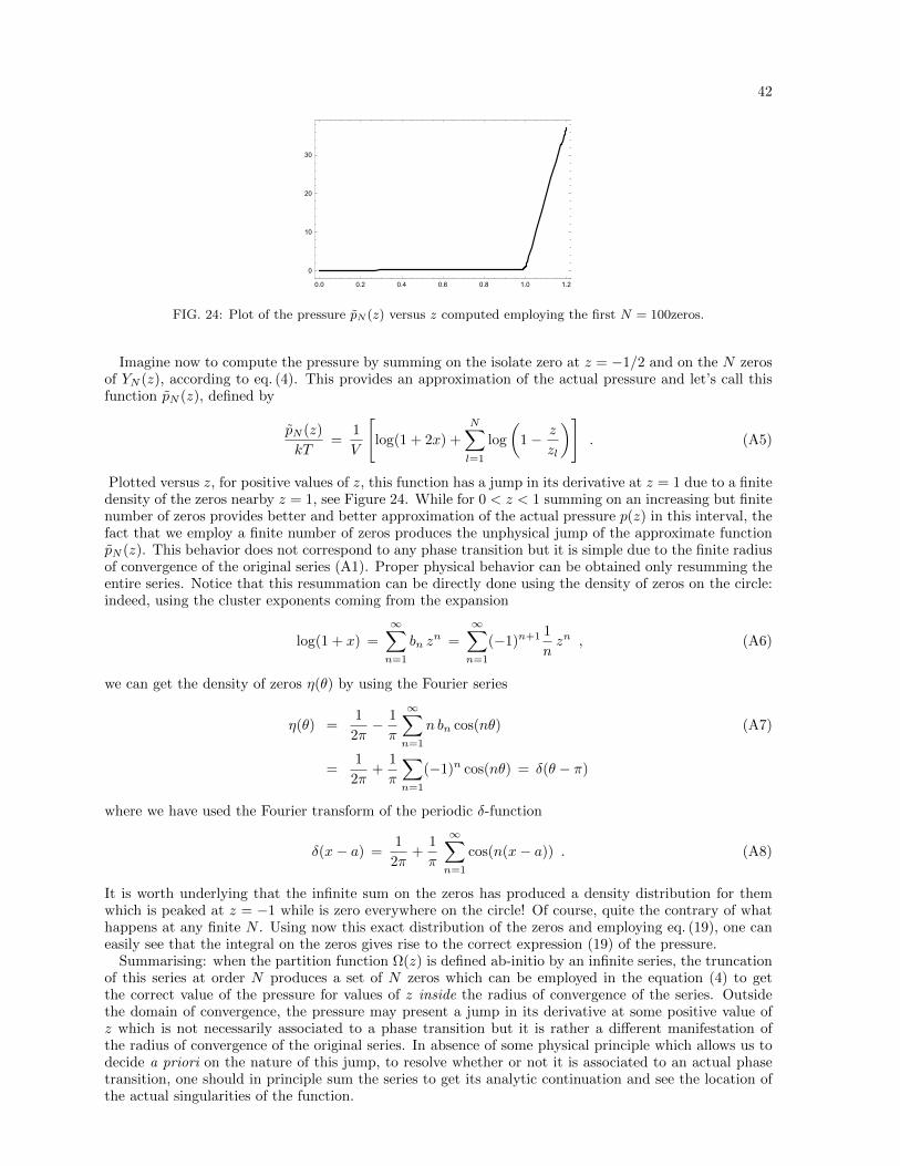
42
FIG. 24: Plot of the pressure pN (z) versus z computed employing the first N = 100zeros.
Imagine now to compute the pressure by summing on the isolate zero at z = −1/2 and on the N zerosof YN (z), according to eq. (4). This provides an approximation of the actual pressure and let’s call thisfunction pN (z), defined by
pN (z)
kT=
1
V
[log(1 + 2x) +
N∑l=1
log
(1− z
zl
)]. (A5)
Plotted versus z, for positive values of z, this function has a jump in its derivative at z = 1 due to a finitedensity of the zeros nearby z = 1, see Figure 24. While for 0 < z < 1 summing on an increasing but finitenumber of zeros provides better and better approximation of the actual pressure p(z) in this interval, thefact that we employ a finite number of zeros produces the unphysical jump of the approximate functionpN (z). This behavior does not correspond to any phase transition but it is simple due to the finite radiusof convergence of the original series (A1). Proper physical behavior can be obtained only resumming theentire series. Notice that this resummation can be directly done using the density of zeros on the circle:indeed, using the cluster exponents coming from the expansion
log(1 + x) =
∞∑n=1
bn zn =
∞∑n=1
(−1)n+1 1
nzn , (A6)
we can get the density of zeros η(θ) by using the Fourier series
η(θ) =1
2π− 1
π
∞∑n=1
n bn cos(nθ) (A7)
=1
2π+
1
π
∑n=1
(−1)n cos(nθ) = δ(θ − π)
where we have used the Fourier transform of the periodic δ-function
δ(x− a) =1
2π+
1
π
∞∑n=1
cos(n(x− a)) . (A8)
It is worth underlying that the infinite sum on the zeros has produced a density distribution for themwhich is peaked at z = −1 while is zero everywhere on the circle! Of course, quite the contrary of whathappens at any finite N . Using now this exact distribution of the zeros and employing eq. (19), one caneasily see that the integral on the zeros gives rise to the correct expression (19) of the pressure.
Summarising: when the partition function Ω(z) is defined ab-initio by an infinite series, the truncationof this series at order N produces a set of N zeros which can be employed in the equation (4) to getthe correct value of the pressure for values of z inside the radius of convergence of the series. Outsidethe domain of convergence, the pressure may present a jump in its derivative at some positive value ofz which is not necessarily associated to a phase transition but it is rather a different manifestation ofthe radius of convergence of the original series. In absence of some physical principle which allows us todecide a priori on the nature of this jump, to resolve whether or not it is associated to an actual phasetransition, one should in principle sum the series to get its analytic continuation and see the location ofthe actual singularities of the function.
43
Appendix B: Plateau value of the Thermodynamics Bethe Ansatz equations
In this Appendix we derive the plateau value ε0(z) of the pseudo-energy by using the kink-solution ofthe Thermodynamics Bethe Ansatz equation and the value of the free energy at β = 0. The kink solutionemerges when β → 0 and concerns the behavior of ε(θ, z) nearby the edge θ ' Λ(β) = log(2/β): it solvesthe non-linear integral equation
εkink(θ) = eθ − 1
2π
∞∫−∞
dθ′ϕ(θ − θ′) ln(
1 + ze−εkink(θ′)
), (B1)
and it allows to compute the free energy at β = 0
f(z) = − 1
π
∞∫−∞
eθ ln(
1 + ze−εkink(θ′)
). (B2)
Using some standard steps (see for instance [19]), this expression can be also written as
f(z) =1
2π
∞∫ε0
dε
[εzeε
1 + ze−ε+ ln
(1 + ze−ε
)]. (B3)
The lower bound of the integral ε0(z) is the value of the pseudo-energy at the plateau and for the Yang-Leemodel it is solution of the non-linear equation
ε0(z) = ln(
1 + ze−ε0(z)). (B4)
If we define x0 ≡ eε0 , we obtain the equation:
x0 = 1 +z
x0
x20 − x0 − z = 0 (B5)
x0 =1 +√
1 + 4z
2
where we have taken the positive solution of the quadratic equation. We can now make a change ofvariable in the integral (B2) in terms of
y =ze−ε
1 + ze−ε(B6)
so that the extrema of the integral become:
y− =ze−ε0
1 + ze−ε0=
z
eε0 + z=
z
x0 + z, (B7)
y+ = 0 . (B8)
With this substitution we also have:
ε = ln(1− y)− ln y − ln z , (B9)
so that
dε =
(1
1− y− 1
y
)dy = − dy
y(1− y)(B10)

44
Therefore
f(z) =1
2π
0∫y−
dy
y(1− y)[y (ln(1− y)− ln y − ln z)− ln(1− y)] =
=1
2π
0∫y−
dy
y(1− y)[(y − 1) ln(1− y)− y ln y − y ln z] =
=1
2π
− 0∫y−
dy
yln(1− y)−
0∫y−
dyln y
(1− y)
− 1
2π
0∫y−
ln z
(1− y)dy =
= − 1
π
−1
2
y−∫0
dy
yln(1− y)−
y−∫0
dyln y
(1− y)
− 1
2π
0∫y−
ln z
(1− y)dy (B11)
The function within the square parenthesis is the Rogers Dilogarithmic function L(y−) = L (z/(z + x0))and therefore
f(z) = − 1
πL
(z
z + x0
)− 1
2π
0∫y−
ln z
(1− y)dy
= − 1
πL
(z
z + x0
)+
1
2πln z
(ln (1− y) |0y−
)=
= − 1
πL
(z
z + eε0
)− 1
2πln(z) ln
(x0
x0 + z
)=
= − 1
πL
(z
z + 1+√
1+4z2
)− 1
2πln(z) ln
(1+√
1+4z2
1+√
1+4z2 + z
). (B12)
45
[1] T. Regge, Il Nuovo Cimento Series 10, Vol. 14, 1959, p. 951.[2] C. N. Yang, T. D. Lee, Phys. Rev., 87, 404 (1952).[3] T.D. Lee, C. N. Yang, Phys. Rev. 87, 410 (1952).[4] T. Asano, Progr. Theoret. Physics (Kyoto) 40, 1328 (1968); J. Phys. Soc. Japan 25, 1220 (1968).[5] J. Math. Phys. 9, 2064 (1968); Progr. Theoret. Physics (Kyoto) 40, 1246 (1968).[6] R.B. Griffiths, J. Math. Phys. 10, 1559 (1969).[7] M. Suzuki and M. Fisher, J. Math. Phys. 12, 235 (1971).[8] P.J. Kortman and R.B. Griffiths, Phys. Rev. Lett. 27, 1439 (1971).[9] M. E. Fisher, Phys. Rev. Lett. 40, 1610 (1978).
[10] J.L. Cardy and G. Mussardo, Phys. Lett. 225, 275 (1989).[11] J.L. Cardy, Phys. Rev. Lett. 54 (1985) 1354.[12] C. M. Bender, V. Branchina, E. Messina, Phys.Rev. D87 (2013), 085029.[13] Al. B. Zamolodchikov, Nucl. Phys. B 348 (1991) 619.[14] A.B. Zamolodchikov and Al.B. Zamolodchikov, Annals Phys. 120 (1979) 253-291.[15] A. B. Zamolodchikov, Adv.Stud.Pure Math. 19 (1989) 641-674.[16] G. Mussardo, Statistical Field Theory, Oxford University Press, 2010.[17] Al.B.Zamolodchikov, Nucl. Phys. B 342 (1990) 695.[18] V.P. Yurov and Al.B. Zamolodchikov, Int.J.Mod.Phys. A5 (1990) 3221-3246[19] P. Fendley, Nucl. Phys. B 374 (1992) 667.[20] T.R. Klassen and E. Melzer, NucI. Phys. B350 (1990) 635.[21] J.E. Mayer, J. Chem. Phys. 5, 67 (1937); J.E. Mayer and Ph.G. Ackermann, J. Chem. Phys. 5, 74 (1937);
J.E. Mayer and S.F. Harrison, J. Chem. Phys. 7, 87,101 (1938).[22] K. Huang, Statistical Mechanics, II edition, Wiley and sons.[23] D.C. Mattis, The theory of magnetism made simple, World Scientific Publishing Co. (Singapore) 2006.[24] I. Bena, M. Droz, A. Lipowski, Int. J. Mod. Phys. B 1, 4269 (2005).[25] R.A. Blythe and M.R. Evans, Braz. J. Phys. 33, 464 (2003).[26] K. Ikeda, Prog. Theor. Phys. 58, 496 (1977); Prog. Theor. Phys. 61, 27 (1979).[27] K. Ikeda, Progr. Theor. Phys. Vol. 68, 461 (1982)[28] K. Ikeda, Progr. Theor. Phys. Vol. 68, 744 (1982).[29] R. Abe, Prog. Theor. Phys. 38, 72 (1967).[30] R. Abe, Prog. Theor. Phys. 38, 568(1967).[31] S. Katsura, J. Chem. Phys. 22, 1277 (1954); Prog. Theor. Phys. 13, 571 (1955).[32] P. Fonseca and A.B. Zamolodchkov, J. Stat. Phys. 110 (2003) 527.[33] T. Wydro and J. Mccabe, Yang-Lee singularity of two dimensional Ising and Potts model, in in Symmetry
and Structural Properties of Condensed Matter, 9 (World Scientific, Eds. T. Lulek, B. Lulek, and A. Wal2003).
[34] A. Mossa and G. Mussardo, J.Stat.Mech. 0803 (2008) P03010.[35] M. Assis, J.L. Jacobsen, I. Jensen, J-M. Maillard and B.M. McCoy, Analyticity of the Ising susceptibility: An
interpretation, arXiv:1705.0254.[36] X. Ana, D. Mesterhazyb, and M. A. Stephanov, On spinodal points and Lee-Yang edge singularities,
arXiv:1707.06447.[37] Ch. Binek, Phys. Rev. Lett. 81, 5644 (1998); Ch. Binek, W. Kleemann and H.A. Katori, J. Phys. Condens.
Matter 13 (2001), L811.[38] B.B. Wei and R.B. Liu, Phys. Rev. Lett. 109, 185701 (2012); B.B. Wei, S.W. Chen, H.C. Po and R.B. Liu,
Sci. Rep. 4, 5202 (2014).[39] X. Peng, H. Zhou, B.B. Wi, J. Cui, J. Du, R.B. Liu, Phys. Rev. Lett. 114, 010601 (2015).[40] V.V. Prasolov, Polynomials, Springer-Verlag Berlin Heidelberg 2004.[41] D. Zagier, The dilogarithm function in Frontiers in Number Theory, Physics, and Geometry II, Springer
2007; A.N. Kirillov, Dilogarithm identities, in Quantum field theory, integrable models and beyond, Kyoto1994, Progress of Theoretical Physics Supplement 118 (1995) 61.
[42] A. Leclair and G. Mussardo, Nucl. Phys. B 552 (1999) 624.[43] R. Koberle and J.A. Swieca, Phys. Lett. B 86B, 209 (1979).[44] V.P. Yurov and Al.B. Zamolodchikov, Int. J. Mod. Phys. A6 (1991), 3419.[45] Al. B. Zamolodchikov, Int.J.Mod.Phys. A10 (1995) 1125; J.Phys. A39 (2006) 12863-12887.[46] G. Mussardo and P. Simon, Nucl.Phys. B578 (2000) 527.