c� 2010 Min-Yang A. Lee

THREE ESSAYS ON FISHERIES ECONOMICS

BY

MIN-YANG A. LEE

DISSERTATION

Submitted in partial fulfillment of the requirementsfor the degree of Doctor of Philosophy in Agriculture and Consumer Economics

in the Graduate College of theUniversity of Illinois at Urbana-Champaign, 2010

Urbana, Illinois

Doctoral Committee:

Associate Professor Richard J. Brazee, Chair and Director of ResearchAssociate Professor Amy W. AndoProfessor John B. BradenEric M. Thunberg, NOAA Fisheries

Abstract

This dissertation examines three themes of efficiency in fisheries economics and man-

agement. The first theme is intertemporal efficiency; by examining fishery management

problems within a stochastic bioeconomic model, the tradeoffs between current and future

consumption are clear. The second theme explored in this essay is the efficiency of trad-

able permits system in the presence of trade restrictions. The third theme explored in this

dissertation is efficiency in the presence of ecosystem externalities.

Fisheries managers must often make decisions even while there is large amounts of

uncertainty regarding stock level; furthermore, there are often fairly long periods of time

in which they are unable to assess stock levels. The first essay examines a bioeconomic

fishery model that includes rigidity in the policy-setting process, a management reality that

has yet to be incorporated into these types of models. Although analytically intractable, the

model is simulated across a range of biological and institutional parameters to learn how

this rigidity affects the manager’s optimization problem. While the effects of rigidity with

deterministic stock growth are shown to be small; when growth is stochastic, the present

value of fisheries revenue may drastically decline under rigid management. By solving

for the present value of fisheries revenues across a wide range of parameter values, the

economic tradeoffs between management and scientific activities can be clarified.

The second essay examines bilateral bargaining in a market for a unique synthetic input

permits, Days-at-Sea, in the Northeast groundfish fishery. This research applies a quantile

regression approach to the estimation of bargaining power and tests a key identification

assumption of bargaining power equality made by previous researchers. One of the findings

ii

of this research is that current regulations may have segmented this market, endowing some

firms with bargaining power relative to others.

The final essay examines a small ecosystem-economy in which there are competing

extractive and non-extractive uses for the fishery resource. In this ecosystem, herring are

commerically harvested and are food for whales, which are an input in a non-extractive

tourism industry, whale-watching. A finding of this research is that fishing negatively im-

pacts the whale-watching industry; however, the magnitude of these effects are small. The

results contained in this essay are useful inputs for managers seeking to implement Ecosys-

tem Based Fishery Management.

iii

To Diana.

iv

Acknowledgments

This dissertation would not have been possible without the invaluable help of my disserta-

tion committee.

The majority of this research was conducted while I was a Sea Grant-NMFS Fellow

in Marine Resource Economics. Staff at the Northeast Fisheries Science Center have been

particularly helpful and supportive. A portion this research was also funded by a University

of Illinois Graduate College Dissertation Travel Grant. I would also like to thank the Blue

Ocean Society for Marine Conservation, Ocean Alliance, the Center for Oceanic Research

and Education for providing whale-watching data.

v

Table of Contents

Chapter 1 Introduction . . . . . . . . . . . . . . . . . . . . . . . . . . . . . . . 1

1.1 Fishery Management in the United States . . . . . . . . . . . . . . . . . . 1

1.2 Three Essays on Fisheries Economics . . . . . . . . . . . . . . . . . . . . 4

Chapter 2 The Effects of Policy Rigidity on Optimal Fisheries Management . . 8

2.1 Introduction . . . . . . . . . . . . . . . . . . . . . . . . . . . . . . . . . . 8

2.2 Policy Rigidity and Uncertainty . . . . . . . . . . . . . . . . . . . . . . . 13

2.3 Methods . . . . . . . . . . . . . . . . . . . . . . . . . . . . . . . . . . . . 16

2.4 Results and Discussion . . . . . . . . . . . . . . . . . . . . . . . . . . . . 18

2.5 Conclusions . . . . . . . . . . . . . . . . . . . . . . . . . . . . . . . . . . 22

2.6 Tables and Figures . . . . . . . . . . . . . . . . . . . . . . . . . . . . . . 25

Chapter 3 Bargaining for Homogeneous Goods:

The Days­at­Sea Market . . . . . . . . . . . . . . . . . . . . . . . . . . . . . . 34

3.1 Introduction . . . . . . . . . . . . . . . . . . . . . . . . . . . . . . . . . . 34

3.2 The Days-at-Sea Market . . . . . . . . . . . . . . . . . . . . . . . . . . . 38

3.3 Empirical Model and Data Used . . . . . . . . . . . . . . . . . . . . . . . 42

3.4 Results . . . . . . . . . . . . . . . . . . . . . . . . . . . . . . . . . . . . . 46

3.5 Conclusions . . . . . . . . . . . . . . . . . . . . . . . . . . . . . . . . . . 51

3.6 Tables and Figures . . . . . . . . . . . . . . . . . . . . . . . . . . . . . . 53

Chapter 4 Economic Tradeoffs in the Gulf of Maine Ecosystem: Herring and

Watching . . . . . . . . . . . . . . . . . . . . . . . . . . . . . . . . . . . . . . 76

4.1 Introduction . . . . . . . . . . . . . . . . . . . . . . . . . . . . . . . . . . 76

4.2 Background . . . . . . . . . . . . . . . . . . . . . . . . . . . . . . . . . . 77

4.2.1 The Whale-watching Industry . . . . . . . . . . . . . . . . . . . . 77

4.2.2 The Herring Fishery . . . . . . . . . . . . . . . . . . . . . . . . . 78

4.3 Modeling Approach . . . . . . . . . . . . . . . . . . . . . . . . . . . . . . 79

4.4 Data and Econometric Model . . . . . . . . . . . . . . . . . . . . . . . . . 81

4.5 Results and Discussion . . . . . . . . . . . . . . . . . . . . . . . . . . . . 85

4.6 Conclusions and Future Research . . . . . . . . . . . . . . . . . . . . . . . 89

4.7 Tables and Figures . . . . . . . . . . . . . . . . . . . . . . . . . . . . . . 91

Chapter 5 Conclusions . . . . . . . . . . . . . . . . . . . . . . . . . . . . . . . . 95

Appendix A Logistic Growth and a 2 Year Planning Period . . . . . . . . . . . 97

vi

Appendix B Numerical Methods for Dynamic Programming . . . . . . . . . . 99

Appendix C Days­at­Sea Leasing . . . . . . . . . . . . . . . . . . . . . . . . . . 101

References . . . . . . . . . . . . . . . . . . . . . . . . . . . . . . . . . . . . . . . 114

vii

Chapter 1

Introduction

Economists have typically addressed three major issues in the field of fishery manage-

ment: intertemporal efficiency, allocative efficiency of markets, and efficient production

in the presence of externalities. This dissertation is composed of three essays that address

these topics. The first essay examines the effects of stock-growth uncertainty and pol-

icy rigidity using a bioeconomic model. Policy rigidity is a management institution that

utilizes a constant control variable (harvest or quota) for a relatively long period of time.

During this time, the stock may experience multiple growth shocks. The second essay

examines bilateral bargaining in the market for Northeast Multispecies Groundfish Days-

at-Sea (DAS). This unique system was initially designed as a simple input control, but has

since evolved into a tradable input control. The DAS market has few, if any characteristics

of a market: prices are not publicly available, speculation is explicitly disallowed, there

are legal limitations that govern potential trading partners, and finding a trading partner

may be costly. The final essay examines a small economy containing extractive (fishing)

and non-extractive uses (whale-watching) as an example of the Ecosystem Based Fisheries

Management (EBFM) approach.

1.1 Fishery Management in the United States

Management of fisheries in the United States is a complex process with many involved par-

ties. Under the Magnuson-Stevens Fishery Conservation and Management Act (MSFCA),

regional Management Councils propose fishery management plans (MSFCA, 2007). The

1

regional Councils are composed of stakeholders, typically fishing industry groups, and are

advised by National Marine Fisheries Service (NMFS) and academics on scientific and

technical issues. Proposed regulations are then adopted and enacted by the Department of

Commerce. The regional Councils are guided by many pieces of legislation, including the

MSFCA, the Marine Mammal Protection Act (MMPA), and the National Environmental

Policy Act (NEPA).

The MSFCA and subsequent amendments establishes 10 “National Standards” or prin-

ciples for fishery management.

1. Management plans should prevent overfishing and achieve Optimum Yield.

2. Managers should use the best available science.

3. Stocks of fish that are interrelated should be managed jointly and individual stocks

should be managed as a single unit.

4. Management measures should not discriminate across states. Permits or priviledges

should be assigned fairly and equitably; furthermore, no entities should acquire ex-

cessive share of those priviledges.

5. Management plans should consider efficiency, but not be solely based on economic

efficiency.

6. Management plans should take variability of stocks and catches into account and

include contingencies.

7. Management plans should minimize costs and duplication of compliance effort.

8. The economic and social impacts on fishing communities should be taken into ac-

count.

9. Management plans should minize bycatch and mortality of bycatch.

10. Management plans should promote safety at sea.

Many of the terms included in these standards are subject to interpretation; however,

Optimum Yield has specifically been defined by Congress. Optimum Yield is defined as

the harvest that produces the greatest net benefits to the United States and equal to the

maximum sustained yield less any reduction for economic, social, or ecological factors.

The last of these, “ecosystem considerations,” has served as motivation for the adoption of

2

Ecosystem Based Fisheries Management (Link, 2002; Pikitch et al., 2004). For stocks that

are overfished, Optimum Yield is defined as the yield that allows for rebuilding stocks to

levels that would produce the maximum sustained yield.

NMFS has produced guidance documents that interpret and operationalize the National

Standards described in the MSFCA (NMFS, 2008). For example, the interpretation of Na-

tional Standard 1 has produced many reference points for fish stocks. Maximum Sustained

Yield (MSY) is defined as the largest long-run average yield of a stock, given ecological

conditions and fishing technology in use. Acceptable Biological Catch (ABC) are catch

levels which account for scientific uncertainty and must be less than Optimum Yield (OY).

An Annual Catch Limit (ACL) is a threshold catch level that must be less than ABC; if

catch rises above this level, Accountability Measures (AMs) are implemented. Together,

ACLs and AMs are intended to act as a deterrent to overfishing. Finally, Annual Catch

Targets (ACTs) are the target harvest rate of managers; these are less than ACLs and are

set to account for management uncertainty.

As a part of the Executive Branch, Department of Commerce regulations are also guided

by Executive Order 12866, which was signed by President Clinton in 1993. Under this

Executive Order, regulatory agencies should assess costs and benefits of alternative reg-

ulations, including costs of enforcement and compliance that are borne by government

agencies. Regulatory actions should maximize net benefits to the United States and use

incentive based systems in place of command-and-control systems when possible. Further-

more, regulatory agencies should use “the best reasonably obtainable scientific, technical,

economic, and other information.”

In 2008, the National Marine Fisheries Service reviewed the status of 531 fish stocks

in the United States to determine whether these stocks were overfished or if overfishing

was occurring (U.S. Department of Commerce, 2009). These determinations were made

on a stock-by-stock basis and relied solely on biological indicators, estimated Maximum

3

Sustained Yield and current harvest levels1. An overfished stock of fish is characterized

by stock levels that are “too low,” while overfishing indicates that current harvest levels

are “too high.” Scientific uncertainty was so large that determination of overfished status

could be made on only 199 of those 531 stocks. Of those 199 stocks of fish, 46 (23%) were

classified as overfished. Determination of overfishing status could be made on only 251

of the 531 stocks reviewed. Of those 251 stocks, 41 (16%) were experiencing overfishing.

Clearly, uncertainty is abundant in fisheries management.

1.2 Three Essays on Fisheries Economics

The first essay in this dissertation examines the impacts of policy rigidity and uncertainty

on optimal fisheries policy and value. Intertemporal efficiency has been examined using

bioeconomic models since the work of Clark (1976). By modeling the fishery as a capital

asset, the tradeoff between present and future consumption is clear: increasing current con-

sumption typically lowers the productivity of the resource and therefore future consump-

tion. The analytical solutions of deterministic models typically lead to a natural resource

“golden rule”: optimal harvest of the resource precisely balances the marginal benefits

of harvest against marginal opportunity costs of harvest that are derived from lower pro-

ductivity. With this rule in hand, it is often possible to solve for the explicit harvest and

stock levels that maximize net benefits. However, analytical solutions often become dif-

ficult to understand with the introduction of stochastic stock growth and/or measurement

error (Clark and Kirkwood, 1986; Costello et al., 2001; Sethi et al., 2005). As noted by

Thompson (1999), the analytical solutions produced by bioeconomic models are complex

and infrequently implemented.

The classical bioeconomic models have assumed that the manager has information

about the present stock size and is able to adjust the harvest or quota levels “quickly”

1These indicators are B�SY - the stock that produces the Maximum Sustained Yield and F�SY - the

harvest rate associated with MSY, along with B and F , the actual stock and harvest rate.

4

(Reed, 1979; Clark and Kirkwood, 1986). However, this may not be a realistic assump-

tion: the slow-moving political bodies may simply be unable to do so. These agencies

may have chosen longer management intervals directly, perhaps to reduce the transactions

costs of management. They may also have chosen them indirectly, through the allocations

of labor and funds to scientific and management activities for various species and stocks

of fish. Both time and money are required for accurate science and management; policy

rigidity may a consequence of these allocation decisions. Examination of the effects of

rigidity and uncertainty on the the present value of the fishery can clarify the embedded

economic tradeoffs between gathering information and proceeding with management ac-

tivities (Hansen and Jones, 2008; Mantyniemi et al., 2009).

The second essay in this dissertation examines the effects of institutional limitations on

bargaining power in a synthetic market. This essay adapts Harding et al.’s (2003) hedonic

bargaining power model to examine how characteristics of buyers and sellers determine

prices for Days-at-Sea (DAS). This tradable effort control system is a synthetic permit

market with many limitations on trade and a lack of an actual marketplace. Once buyers

and sellers match, trades are likely to be negotiated through a bilateral bargaining process.

The industrial-organization literature in this field typically assumes that trade generate eco-

nomic surplus; the two parties bargain over the division of that surplus (Blair et al., 1989).

Harding et al. (2003) make strong identification assumptions; the unique nature of DAS

allows these assumptions to be critically examined.

When stock use is not rationed, either through price or quantity controls, the stock is

typically overused in the production process, causing stock collapse. There are many pos-

sible solutions to the public goods problem: properly calibrated access fees, effort controls,

landings taxes, and aggregate or individual quotas could all be used if the manager has

full information about production technology. Transferable rights based systems, typically

based on output, have become popular as a fisheries management tool to achieve allocative

efficiency (Batstone and Sharp, 2003; Costello et al., 2008). However, input control sys-

5

tems continue to be popular with the fishing industry (Rossiter and Stead, 2003). National

Standard 4 requires management plans and activities to prevent the entities from obtaining

“excessive share” of fishing priviledges. While this term is never defined, a reasonable

interpretation of this may include the ability to exert market or bargaining power. Examin-

ination of bargaining power in this market can provide insight into best practices for other

synthetic markets.

The final essay in this dissertation is examines production in the presence of external-

ities. There are few commercial marine fisheries that are completely isolated. Many are

linked to other commercial fisheries, either through biological (predator-prey) interactions

or through joint production technology in harvest. Others are linked to recreational fish-

eries, non-extractive uses, or non-harvested (but desirable) species. Under the definition

of Optimum Yield in the MSFCA these linkages must be accounted for in setting pol-

icy. Many economic methods have been used to examine and address the interconnections

in the ecosystem, from bioeconomic predator-prey and ecosystem models (Ragozin and

Brown, 1985; Brown et al., 2005; Finnoff and Tschirhart, 2003) to econometric charac-

terization of the joint production technology (Squires, 1987; Squires and Kirkley, 1991).

These economic methods can inform managers as they implement Ecosystem Based Fish-

ery Management (EBFM), in which entire ecosystems, not just a single target species, are

managed (Link, 2002; Pikitch et al., 2004).

Dynamic, long-run bioeconomic models are not always necessary for the implemen-

tation of the EBFM approach to management. This approach also requires knowledge

of short-term ecosystem linkages, especially as they affect human activities. Using the

ecosystem-externality model of Crocker and Tschirhart (1992), this research provides in-

sight into the external effects of fishing activity on a non-extractive tourism industry.

The essays in this dissertation examine three general aspects of efficiency in fisheries

economics and policy. Bioeconomic models can be used to examine intertemporal effi-

ciency issues. Tradable permits are thought to be lead to efficient production; the second

6

essay examines an existing market and provide insight into the effects of market institu-

tions. The Ecosystem Based Management paradigm recognizes that the fishery is just one

use of marine resources; the final essay examines the the short-term effects of fishing on a

non-extractive (tourism) industry.

7

Chapter 2

The Effects of Policy Rigidity on

Optimal Fisheries Management

2.1 Introduction

This essay examines the effects of policy rigidity in a bioeconomic model, with emphasis

on the consequences for fishery value, the optimal policy function, and stock collapse. In

this essay, policy rigidity is defined as a management institution in which the control vari-

able (i.e. quota or Total Allowable Catch) is fixed for the duration of a “short-term planning

period.” During this time, the managed stock may experience multiple growth shocks. Two

stylized facts about fisheries management motivate this research. First, frequent adjustment

of policy has high direct and indirect transactions costs (Turner and Weninger, 2005; Singh

et al., 2006). Policy rigidity may be a direct choice of fishery managers who are influ-

enced by these high transactions costs (Table 2.1). Second, relative to terrestrial resources,

marine fish stocks are difficult to measure and subject to large stochastic growth shocks;

stocks are assessed using combinations of fishery-dependent and independent techniques

that require large amounts of time and money to perform. The scientific assessment process

may result in relatively long periods of time during which the manager lacks information

about the stock size (Table 2.2). Infrequent assessments may be a management strategy that

accounts for the allocation of scarce resources to scientific and management activities for

many species of fish. Without current information about the stock the manager must condi-

tion policy on expectations about stock sizes. Indirectly, the limited amount of information

possessed by managers may constrain them to adopt rigid policies. This management insti-

tution will reduce the present value of fishery revenues; however, the opportunity costs of

8

rigidity are not well understood. This research generalizes the Clark and Kirkwood (1986)

bioeconomic fishery model by introducing a short-term planning period and examining

the tradeoffs between rigidity, information, and fishery value that fishery managers must

consider in the decision-making process.

Under the Magnuson-Stevens Fishery Conservation Act (MSFCA), the National Ma-

rine Fisheries Service (NMFS) provides biological and economic advice to regional Fish-

ery Management Councils that manage fish stocks in United States waters. The major

component of that advice is related to the appropriate level of harvest and set-asides that

account for scientific and management uncertainty. NMFS has produced guidance docu-

ments that interpret and operationalize the National Standards described in the MSFCA

(NMFS, 2008). Maximum Sustained Yield (MSY) is defined as the largest long-run aver-

age yield of a stock, given ecological conditions and fishing technology in use. Optimum

Yield (OY) is Congressionally defined as MSY less allowances for social, economic, and

ecosystem considerations. Acceptable Biological Catch (ABC) are catch levels which ac-

count for scientific uncertainty and must be less than OY. An Annual Catch Limit (ACL) is

a threshold catch level that must be less than ABC. Finally, Annual Catch Targets (ACTs)

are the target harvest rate of managers; these are less than ACLs and must account for man-

agement uncertainty. The findings of this research, particularly the relationship between

policy intervals and optimal harvest and extinction, can be used by managers to set some

of these biological reference points.

Economists have typically constructed bioeconomic models to examine optimal harvest

rates and value from a capital accumulation perspective (Clark, 1976; Reed, 1979; Clark

and Kirkwood, 1986; Conrad and Clark, 1987). Three types of uncertainty were incorpo-

rated into a bioeconomic fishery model by Roughgarden and Smith (1996): growth, mea-

surement, and harvest uncertainty. The first two types of uncertainty correspond to scien-

tific uncertainty, while harvest uncertainty is closely related to the management uncertainty

described in the MSFCA. Sethi et al. (2005) solve the model developed by Roughgarden

9

and Smith (1996) and find that stock measurement uncertainty produces the largest qual-

itative changes in optimal policy. Costello et al. (2001) examine the ability of a manager

to predict future growth stocks and find that prediction of a “good” growth shock leads

to lower current harvests. A predicted good shock implies that the opportunity costs of

harvest are larger than typical. While counterintuitive from a conservation standpoint, a

prediction of a good shock indicates larger returns from allowing that stock to remain in

the ecosystem to grow.

In general, the optimal policy prescribed by a bioeconomic model is a function that

maps the state space to action space. After solving for the optimal policy function, economists

(implicitly) assume that this policy function is simply adopted. The actual level of harvest,

quota, or Total Allowable Catch is then set mechanistically when the uncertainty about the

the stock level is resolved. However, this rarely occurs in fisheries management, especially

when that policy is a complex harvest function (Thompson, 1999). Instead, quota levels are

typically set through a bargaining and negotiation process; these quotas may be fixed for a

period of multiple years. While rigid policy instruments have not been examined in bioe-

conomics models, capital rigidity has previously been incorporated in those models. Singh

et al. (2006) construct a two-stock model (fishing capital and fish stock) to examine the im-

pact of capital rigidity on policy. In that model, capital cannot be removed instantaneously

and fishing capital is specific to the industry. The major finding is that the manager must

balance the additional revenues of a very flexible harvest policy against the costs of con-

stantly adjusting capital; Singh et al. (2006) describe this phenomenon as catch-smoothing.

Within the fisheries management literature there has been recent interest in the value

of information about stock dynamics and the substitutability of management and scientific

activities. Hansen and Jones (2008) examine the tradeoffs between gathering scientific

information and management in a case study of the control of an aquatic pest. Mantyniemi

et al. (2009) examine the benefits of correctly selecting the appropriate stock equation for

herring from a set of possible choices using a Bayesian framework. These concepts have

10

also been explored in the economics literature; Saphores and Shogren (2005) use a real-

options framework to determine the optimal amount of information that should be gathered

before costly actions should be undertaken to control an invasive species.

Many of the key findings of stochastic fishery models were developed by Reed (1979)

and Clark and Kirkwood (1986). Both models implicitly assume that the manager’s only

source of information is an assessment that is conducted prior to the beginning of the fish-

ing season. In Reed’s (1979) model, this assessment occurs after the growth shock has

occurred but before the policy is declared. This assessment perfectly measures the level of

the harvestable stock; the manager can set policy conditional on the harvestable stock. Not

surprisingly, the optimal policy is similar to the optimal policy when growth is determin-

istic and can be characterized as a constant target escapement policy1 (Conrad and Clark,

1987). When stock levels are higher than the target, the entire “surplus” is harvested. When

stock levels are lower, there is no harvest and the stock is allowed to recover to the target

escapement level. The assumption of “real-time” knowledge of the stochastic shock drives

this result and precludes the possibility of accidental extinction.

Clark and Kirkwood (1986) limit the information that the manager possesses by as-

suming that escapement, not harvestable stock, is assessed. A scientific assessment is per-

formed at time t, which perfectly measures St, the escapement at time t. Based on St and

knowledge of the stock dynamics, G�St), the manager selects the harvest quota qt for the

current harvesting season. St grows according to the growth equation into the harvestable

stock, Xt. Harvest occurs, producing the escapement in the next time period, St+1, and the

process repeats infinitely. The manager’s discrete-time optimization problem is to select

1Escapement is amount of fish that has not been harvested in the previous period.

11

the quota in order to maximize the present value of expected fisheries revenues:

maxqt

∞�

t=0

δtpE[ht] (2.1)

Xt = ztG�St) (2.2)

St+1 = Xt − ht (2.3)

ht = min�qt� Xt} (2.4)

In this model, δ ∈ [0� 1) is the per-period discount factor, p is the output price, ht

is harvest, and zt is a multiplicative shock with known distribution φ�zt) that is centered

at unity. Uncertainty enters the model through a stochastic growth function in Equation

(2.2). In the terms of Regan et al. (2002), no distinction is made between natural variation,

inherent randomness, and measurement error in the growth function2. Equation (2.4) can

be interpreted as a feasibility restriction: because the manager does not know the level of

harvestable stock when the quota is declared the harvest must be the lesser of the quota or

the harvestable stock. If, due to a particularly bad growth shock, the declared quota is less

than or equal to the harvestable stock, the stock is driven to extinction. Once the quota is

set, the lesser of the quota or the entire stock is harvested3.

Clark and Kirkwood’s (1986) research advocates precaution when the level of uncer-

tainty is high and finds that the constant-escapement policy is sub-optimal. Because the

harvestable stock is not known when the quota is set, it is theoretically possible for the

manager to set a quota that is higher than the actual stock size and accidentally drive the

stock to extinction.

2While some of this uncertainty is irreducible, scientists and managers have some degree of control over

the uncertainty in the system. For example, additional data could be gathered and incorporated into biological

models, increasing the precision and accuracy of stock assessments.3Clark and Kirkwood (1986) note that this may be an unrealistic assumption. Alternatively, they propose

that harvesting within a season will stop once an arbitrary lower bound, X , is achieved.

12

2.2 Policy Rigidity and Uncertainty

The planning horizon for natural resource problems is typically an infinite or arbitrarily

large number of years, the short-term planning period is defined as a period of k years

during which the policy instrument is held constant. However, the manager still optimizes

the expected present value of the fishery over an infinitely long time horizon.

In this model, a scientific assessment is performed at time t, which perfectly measures

escapement, St. Gk�St� h� z) is the growth function that returns the escapement, St+k, at

the end of the short-term planning period4. The (k × 1) vectors h and z are the harvests

and growth shocks that occur during the short-term planning period. The vector of growth

shocks, z, has known probability distribution φ�z). The growth function Gk�·) is defined

by k- applications of the G�·) as defined in equation (2.2) on St.

Based on measured escapement and knowledge of the stock dynamics, the regulator

selects qj , a harvest quota that is in effect for each year in the jth short-term planning

period. The other main assumptions of the Clark and Kirkwood model remain: harvest (h),

quota (q), and stock size (S) are assumed to be non-negative and E[φ�z)] = 1. The timing

of the Reed, Clark & Kirkwood, and the current model are presented in Figure 2.1.

For short-term planning period of length k, the manager maximizes the expected present

value of the fishery by setting a quota, qj , which is held constant for the duration of the

short-term planning period.

maxq�

∞�

j=0

δkj

k�

i=1

δk�1pE[hi] (2.5)

4Since the planning period is k−years in length, St�k refers to the stock at the time k years or 1 planning

period in the future. More generally, St�mk refers to the stock at the time mk years or m planning periods in

the future.

13

subject to:

St+k = Gk�St� h� z) (2.6)

Xt+i = zt+iG1�St+i�1) ∀i (2.7)

hi = min[qj� Xi] ∀i� j (2.8)

The innovation of the model is contained in Equations (2.5) and (2.6). In equation (2.5), the

“inner” summation produces the discounted expected revenueswithin each short-term plan-

ning period, while the “outer” summation adds these discounted revenues across planning

periods. Equation (2.6) is the stochastic growth equation that maps the initial escapement

level (St), harvests (h), and stochastic shocks (z) to escapement at the end of the short-term

planning period (St+k).

Equations (2.7) and (2.8) function analogously to Equations (2.2) and (2.4) in the Clark

and Kirkwood’s (1986) model. Equation (2.7) describes the harvestable stock at any point

within the short-term planning period. Accidental extinction is possible because the har-

vestable stock of fish (X), is never measured by the manager. Equation (2.8) links the pol-

icy instrument to the stock equation: either the entire quota or the entire harvestable stock

is captured. Both the objective function (Equation 2.5) and the state-transition equation

(2.6) are likely to be non-linear in qj , suggesting that simple constant-escapement policies

are likely to be non-optimal. [XXX quick transition] The Bellman equation can be written

as:

J�t� St; k) = maxq�

�k�

i=1

δ�i�1)pE[hi] + δkE[J�t + k� St+k; k)]} (2.9)

The value function is written as a function of parameter k, the length of the short-term

planning period to make the dependence of J on this parameter more explicit. Solving the

14

Bellman equation provides the following condition for positive quotas:

k�

i=1

[δi�1p∂E[hi]

∂qj

] = δkE[∂J

∂S�t + k�Gk�St� qj); k)]E[

∂Gk

∂qj

�St� qj)] (2.10)

Further algebraic manipulation of equation (2.10) is difficult due to the expectations

operators and minimum function which defines hi. However, Equation (2.10) retains the

traditional “golden rule” interpretation of natural resource economics problems. When the

efficient level of quota is positive, the marginal expected benefits of quota (lhs) must be

equal to the (discounted) marginal expected costs (rhs). These expected costs are equal to

the value of the stock, multiplied by the change in stock productivity.

There are two models of interest that are nested within this bioeconomic model. First,

the Clark and Kirkwood model is a special case of this model in which k = 1. When φ�z)

is degenerate, the model corresponds to policy rigidity with deterministic growth. Second,

when stocks evolve deterministically, the manager’s optimization problem becomes much

simpler. Although the manager chooses qj , quota is always equal to harvest and accidental

extinction is ruled out. The deterministic optimization problem is:

maxq�

∞�

j=0

δkj

k�

i=1

δ�i�1)pqj (2.11)

s.t. St+k = Gk�St� qj).

While the objective function is linear in the control variable, the state transition equation

is linear in qj only if k = 1. Defining a value function J�t� St; k) that is dependent only on

time and escapement provides:

J�t� St; k) = maxq�

�

k�

i=1

[δ�i�1)pqj] + δkJ�t + k�Gk�St� qj); k)} (2.12)

15

Solving the associated Bellman equation when harvesting is positive yields:

k�

i=1

[δi�1p] = δk ∂J

∂S�t + k�Gk�St� hj); k)

∂Gk

∂qj

�St� qj) (2.13)

The summation term on the left-hand side is the marginal benefit of increasing har-

vest levels within the short-term planning period. The right-hand side term captures the

marginal cost of increasing harvest levels: JS�·) is the marginal value of non-harvested

fish and Gkh�·) describes how escapement at the end of the planning period changes with

harvest. Optimal policy requires that the marginal benefits of harvest are equal to marginal

costs of harvest. Appendix A illustrates the model in some depth for logistic growth with a

planning period of 2 years.

2.3 Methods

Numerical simulations are used to understand the effects of policy rigidity on fisheries man-

agement. The goal of these simulations are to understand the combined effects of rigidity

and uncertainty on the value of fisheries revenues, optimal policy, and the possibility of ex-

tinction. In order to isolate the effect of policy rigidity, a deterministic model with rigidity

is first simulated. Next, the stochastic growth model with rigidity is simulated to examine

the combined effects of stochastic growth and rigidity. These simulations are repeated for

a range of biological parameters to better understand the sensitivity of the results to these

parameters.

The discrete-time, discrete-state dynamic programming problem is solved using Mi-

randa and Fackler’s (2002) COMPECON toolbox for MATLAB. Details about the numerical

methods can be found in Appendix B. A discrete-time approximation to logistic growth is

used; the single-year escapement equation is:

St+1 = G�St� zt� ht) = zt[rSt�1−St

K) + St]− ht� (2.14)

16

The annual discount factor (δ) is set to 0.95, and price is normalized to unity. For a

short-term planning period greater than one year in length, repeated application of Equation

(2.14) generates the appropriate state equation (See Appendix B for an illustration). Unless

otherwise noted, the biological parameters, K and r are also set to unity. The K parameter

is typically referred to as carrying capacity; without harvesting or stochastic growth, the

population would evolve to a steady state at K. The r parameter is known as the intrinsic

growth rate; for an arbitrarily-small, positive S, the stock grows at rate r. The speed at

which the stock moves to K is related to both r and the distance of the stock from K.

Under stochastic growth and no harvest, the stock will oscillate around K, with the size of

the oscillations related to all 3 parameters (r�K, and ε). The state equation is symmetric

with respect to K, which may be somewhat unrealistic. zt is assumed to be independently

and identically distributed from a uniform distribution with support [1− ε� 1 + ε], where ε

is varied on the range [0� 0.9].

Let q�S; k) be the quota function that solves equation (2.9) for a given policy interval k.

Similarly, let J�S� q�S; k); k) = J�S; k) be the optimized value of the equation (2.9). The

model is solved for both the optimal policy, q�S; k), and the corresponding expected value

of fisheries revenues, J�S; k), for short-term planning periods of one, two and three years

in length (k = 1� 2� 3). The level of growth uncertainty and the length of the short-term

planning period are treated as parameters in the model. By examining the sensitivity of

the value function to changes in those parameters, it is possible to examine the costs and

benefits of alternative management institutions. For example, holding all other parame-

ters constant, changes in the length of the short-term planning period, k, give insight into

the costs of different management institutions and the possible economic gains from flex-

ible management. Similarly, changes in ε provide insight into the value of more accurate

knowledge of stock dynamics.

17

2.4 Results and Discussion

When stock growth is deterministic, policy rigidity has only a minimal effect on the value of

fishery revenues. The percentage difference in the present value of stock S under different

planning periods can be written as:

ΔJlm =J�S; l)− J�S;m)

J�S; l))

Figure 2.2 plots ΔJlm for l = 1 and m = 2� 3. When growth is deterministic, rigidity pro-

duces only small decreases in the value of the fishery. Intuition for this result can be drawn

from deterministic fishery models: when stocks evolve deterministically, the constant es-

capement target rule and Most Rapid Approach Path are optimal (Conrad and Clark, 1987).

Once the target escapement level is achieved, rigidity cannot have an impact on either pol-

icy or the fishery value. The effects of rigidity are confined to the k−year transition to the

target escapement level. The reductions in the value function are the consequence of mov-

ing “too slowly” to that escapement level. With policy rigidity, the deterministic fishery

also takes the Most Rapid Approach Path to the target escapement. However, this is the

length of the short-term planning period, k-years, instead of a single year. In contrast to

a model with deterministic growth, stochastic growth can produce large economic losses

under policy rigidity. The relative decrease in fishery revenues is robust to the initial stock

size �S0); for this set of biological and economic parameters evaluated, policy rigidity pro-

duces economic losses of twenty or thirty percent when two- or three-year planning periods

are used and ε = 0.5.

The sensitivity of the fishery value to uncertainty is examined in Figure 2.3 by plotting

the optimized value, J�S0 = 0.5; k), as a function of ε, the uncertainty parameter5. The

vertical distance between curves in Figure 2.3 is the change in fishery value that can be

5When stock growth is deterministic, S0 = �.5 is the biomass that produces the Maximum Sustainable

Yield (MSY) for this set of parameters. This stock level is commonly referred to as B�SY . Using initial

values of S0 = �.2� �.8, and 1 does not produce qualitatively different results.

18

attributed to policy rigidity. Consider a fishery for which ε = 0.5 and policy is set every

two years (point A). Adoption of flexible management institutions would move the fishery

to point B, increasing the value of the fishery. Rigidity always reduces the value of the

fishery; this effect is fairly small when stock growth uncertainty is either low or extremely

high. However, at moderate and large levels of uncertainty, policy rigidity causes fairly

large economic losses. This result suggests that rigid policies are best utilized when stock

dynamics are well known and subject to little natural variation.

Movements along a curve in Figure 2.3 represent changes in fishery value due to changes

in the amount of uncertainty in the stock growth equation. The uncertainty parameter (ε)

may be partially under the control of fisheries managers (Regan et al., 2002). For example,

additional scientific effort may increase the knowledge of the growth function, effectively

reducing ε. Reductions in ε always lead to higher value of the fishery. If uncertainty in the

growth function is reduced from ε = 0.5 to ε = 0.4, this would move the fishery from point

A to point C, increasing the value of the fishery. Figures 2.4 and 2.5 are analogous figures

for r = 0.5 and r = 1.5 respectively. The general shapes of the curves in Figures 2.3-2.5

are very similar, changes in r appear to scale the value of the fishery.

While the manager must fix the quota level for the duration of the short-term planning

period, the causes that drive the use of a rigid policy lead to slightly different interpretations

of these figures. When policy rigidity is a direct choice of managers, changes in fishery

value directly reflect the opportunity costs of policy rigidity: Figures 2.3-2.5 make the

opportunity costs of those decisions clear and highlight the biological parameters for which

those institutions are particularly costly. Holding the level of uncertainty constant, these

simulations suggest that stocks with a high intrinsic growth rates (r) relative to K will see

the largest decline in fishery value when using rigid policy.

The model is consistent with an alternative interpretation: an informational constraint

on decision-making due to infrequent stock assessments. If stock assessments are per-

formed every k-years but policy adjusted more frequently, then managers are indirectly

19

constrained to set policy infrequently as well. The manager only knows the probability

distribution from which the shocks are drawn. During years when stock assessments are

not performed, managers are unable to condition quota on the most recent escapement

level. Instead, they must use expectations of stock levels to set policy; this is equivalent

to declaring a multi-year policy at the time that the stock assessment is performed. Under

this interpretation, Figures 2.3-2.5 can provide insight into the implied tradeoffs between

speed and precision in the scientific and management activities. Suppose that there are two

types of recurring scientific activities that can be used to learn about stock dynamics. The

first type can be undertaken rapidly; however, it is associated with larger errors in the stock

equation (ε is larger). The second type of activity takes longer amounts of time; however,

it can explain more the stock dynamics. While assessment and management costs are not

modeled directly in this research, the relative costs and benefits of either approach can be

examined in Figures 2.3-2.5.

Figure 2.6 plots the elasticity of the value function with respect to the growth uncer-

tainty for a stock with biological parameters r = 1 and K = 1.6. This elasticity peaks

when uncertainty is fairly high. The location of this peak is slightly sensitive to the length

of the planning period and occurs at lower levels of uncertainty when k is larger. This high-

lights the tradeoffs inherent in this bioeconomic model; for moderate and large amounts

of uncertainty, there are increasing returns to increasing knowledge of the stock growth

equation, the elasticity is much larger than unity. However, the elasticity of uncertainty

drops below unity at fairly large levels of uncertainty. For values of ε less than this critical

point, further reductions in uncertainty produce decreasing returns. At these lower levels of

uncertainty, it may be optimal to adjust policy faster instead of focusing on reducing stock

growth uncertainty. The exact location of the point at which this occurs depends on the

opportunity costs of uncertainty in Figure 2.3 and the costs of scientific research, which are

not explored in this essay.

6This is approximated as η =ΔV

Δε

ε

V.

20

The optimal quota, conditional on a set of biological parameters and the amount of

rigidity in the system, may be associated with a positive probability of extinction or col-

lapse. As noted by Clark (1973), certain combinations of biological growth and economic

parameters imply that immediate harvest of the entire stock is optimal; however, these sets

of biological and economic parameters are not considered in these simulations. Surpris-

ingly, extinction has received limited attention in the stochastic fishery models; many of

the stochastic fishery models are based on Reed’s (1979) fishery model, which precludes

extinction.

Simulation of the state path is used to gain insight into the probability of extinction.

Using an initial value of (S0 = 0.5), the path of the fishery regulated by the optimal policy

is simulated 1,000,000 times for a 100-year period at varying levels of policy rigidity and

uncertainty. Tables 2.3 and 2.4 present the probabilities that a stock with given parame-

ters will be extinct within a 100 year period under standard (r = 1) and low (r = 0.5)

intrinsic growth rates. These simulations find that extinction does not occur when rigidity

is not present unless uncertainty is extremely high. However, when the stock is managed

with a rigid policy instrument, extinction may occur in the presence of moderate levels of

uncertainty.

When the optimal policy is associated with a positive probability of extinction, it is

difficult to classify extinction events as either accidental or purposeful. By definition, the

optimal policy, q, maximizes the discounted expected revenues in Equation (2.5). These

probabilities of extinction are a result of an optimization process in which the manager is

risk neutral, discounts future fishery revenues at a positive rate, and faces no additional

penalty from extinction beyond the inability to harvest the stocks. In this model, a positive

probability of extinction is accepted in return for higher harvests; this is a byproduct of

managing stocks under policy rigidity with limited information. These findings may par-

tially explain historical fisheries collapse when stock growth is not well understood (ε is

high) or if quota levels are infrequently adjusted (k is high). If stock levels are measured

21

infrequently or quota levels cannot be updated quickly, the extinction occurs with fairly

high probability, even if quota is chosen optimally. This highlights the need for timely,

accurate assessment and management activities.

Two interesting features of the optimal quota function are illustrated in Figure 2.7. The

optimal quota function is symmetric about the carrying capacity; this result is driven by the

symmetry of the growth equation that is used. Healthy stock levels that are near carrying

capacity indicate that future stock levels will also be fairly high. Unhealthy stock levels

that are far from the carrying capacity indicate that future stock levels will be low. Because

of the symmetry of the growth equation, both very low (S near 0) and very high (S near

2K) are unhealthy and will lead to low expected stock levels in the next time period. When

stock levels are healthy, rigidity leads to precautionary quota levels; the optimal quota under

under rigid management is less than the optimal quota for flexible management. However,

this result is reversed for the relatively small interval that correspond to either extremely

low or high stock levels. When constrained to use a rigid policy, the fishery manager prefers

slightly higher quota levels over these intervals.

There is also a threshold stock level at which the fishery is closed. This level depends on

the level of rigidity used to manage the fishery. Both findings can be partially explained by

the way that rigidity is modeled; for computational purposes the quota levels are required

to be constant during the entire short-term planning period. When rebuilding a stock from

unhealthy levels under rigidity, a low level of harvesting is preferred to zero harvest. These

results are also consistent with Singh et al.’s (2006) finding that capital rigidity in the fishery

produces “catch-smoothing.”

2.5 Conclusions

This chapter has examined the effect of a single modification, policy rigidity, to a bioe-

conomic fisheries model with uncertainty. A few stylized facts about management under

22

policy rigidity emerge. Rigidity has limited impact when stock growth uncertainty is small

and no practical impact when stock growth is deterministic. However, both optimal pol-

icy and the value of fisheries revenues are highly sensitive to management rigidity when

growth is highly stochastic. These results suggest that rigid policies, if they must be used,

should be confined to stocks where the dynamics are well understood and subject to little

variation. The combination of rigidity and stochastic growth can have large consequences

for fishery collapse or extinction, even when managed to maximize the net present value of

the fishery. When managers are unable to respond quickly to growth shocks, either because

they are unmeasured or because of rigidity in management, the present value of the fishery

decreases and the probability of collapse increases, sometimes dramatically. These findings

advocate for the explicit consideration for the speed at which policy itself can meaningfully

be changed when setting fisheries policy.

The model as formulated requires the manager to select a harvest level that is constant

within the short-term planning period. This strong assumption about the type of rigidity is

made for computational simplicity to reduce the dimensionality of the dynamic program-

ming problem. However, a weaker version policy rigidity is possible. Under this “weak

rigidity,” the quota level is not necessarily constant for the duration of short-term planning

period; instead, it must only be declared at the beginning of the short-term planning period.

For example, consider a stock that grows deterministically and is far below the desired

level. Under the strict definition of policy rigidity employed in the paper, the optimal pol-

icy may be to harvest at a constant low level for the duration of the short-term planning

period that produces a target escapement level at the end of that period. However, under

a weaker version of rigidity, optimal policy may be to close the fishery for a portion of

the short-term planning period and then allow a higher harvest level short-term planning

period.

The model of rigidity in this essay is similar to the managment procedure for Atlantic

Herring (U.S. National Archives and Records Administration, 2007). In the Northeast

23

United States, the major components of the Atlantic Herring Fishery Management Plan,

including Total Allowable Catch, are specified every three years. Historically, these have

been constant for those three years; however, this is not mandatory. During the three year

planning period, adjustments are possible if warranted by new information. However, new

information can only be obtained by the manager at infrequent intervals; stock assessments

are performend infrequently (Table 2.2).

The bioeconomic model, as formulated, allows instantaneous biological extinction - if

quota levels are mistakenly set above the actual stock size, the fishery collapses immedi-

ately. Immediate biological extinction is unlikely in practice; at a depleted stock level,

fishing would become unprofitable and the directed fishery would shut down for economic

reasons. Interpretation of biological extinction in this model as end of a viable commer-

cial fishery is more realistic. With limited information or ability to control harvest, a stock

may be quickly reduced to levels at which a large-scale, directed fishery is no longer prof-

itable. This research suggests that stocks which grow slowly, are susceptible to large growth

shocks, or are monitored infrequently may be particularly vulnerable to commercial extinc-

tion. The Atlantic Halibut fishery in the northeast United States is an historical example of

this phenomenon (Col and Legault, 2009; Grasso, 2008). This species grows slowly and

was subject to intense fishing in the mid 1800s, resulting in stock collapse by the 1870s.

Both stock size and harvest rates are currently very low and rebuilding of the halibut stock

is complicated because it is a bycatch species in the bottom trawl fishery.

The model used in this essay has abstracted away from costly harvesting in order to

isolate the effect of policy rigidity. This assumption may be non-trivial; if harvest is costly

and depends on the stock level, then observation of the costs of harvest in real-time could

increase the manager’s information about current stock levels. If the cost or production

function is known, managers could use this relationship to determine stock sizes (Smith

et al., 2009). However, this would require large amounts of information and it is unclear

whether these data could be used in a timely manner. It is certainly possible that analysis of

24

economic data requires as much, if not more, time as analysis of fisheries population data.

While this research shows that policy rigidity reduces the value of the fishery, there are

benefits to rigidity that are not incorporated in the model. Firstly, both stock assessments

and management activities are costly; there is likely to be an optimal mix of scientific and

management activities that should be performed (Hansen and Jones, 2008). The precise

point at which this occurs depends on the production of scientific knowledge about the

stocks of fish, which is beyond the scope of this research. Secondly, the avoidance of the

capital adjustment and other transactions costs studied by Singh et al. (2006) may be an

important benefit of managing fish stock using a rigid policy instrument.

2.6 Tables and Figures

Short-Term Landings Value

Species Planning Period (1,000s mt) (�M)

Sea Scallop 2 years 27 �385

Atlantic Herring 2 years 73 �19

Skates 2 years 13 �7

Red Crab 2 years 1 �3

Ocean Quahog 3 years 15 �19

Tilefish 3 years 1 �4

Spiny Dogfish 3 years 3 �1

Table 2.1: Short-Term Planning Period length, landings, and value for selected stocks in

the Northeast United States.

Atlantic Herring Cod (Georges Bank) Sea Scallop

2008 2008 2006

2006 2005 2004

Year 2003 2002 2001

1998 2001 1999

1996 2000 1997

Table 2.2: Recent stock assessments dates for select fisheries in the Northeast United States.

25

Figure 2.1: Timing of actions in the Reed (top), Clark and Kirkwood (middle), and Lee

(bottom) bioeconomic models.

26

0 0.2 0.4 0.6 0.8 10

5

10

15

20

25

30

35

40

45

50

Initial Stock (S0)

Percentage Decrease in Present Value of Fishery Revenues

 

 

k=2, ε=0

k=2, ε=0.5

k=3, ε=0.0

k=3, ε=0.5

Figure 2.2: The impact of policy rigidity and stochastic growth on the present value of

fishery revenues. Logistic stock growth with r = 1� K = 1 ,and δ = .95.

27

0 0.1 0.2 0.3 0.4 0.5 0.6 0.7 0.8 0.90.5

1

1.5

2

2.5

3

3.5

4

4.5

5

5.5

ε

Present Value of Fishery Revenues

 

 

 

k=1

k=2k=3

A

B

C

Figure 2.3: Present value of Fishery Revenues for one-, two-, and three-year planning pe-

riods. Point A corresponds to a fishery which is managed using a 2 year planning period

and ε = 0.5. Point B is a fishery which is managed using a 1 year planning period with

the same level of uncertainty. Point C is a fishery which is managed using a 2 year plan-

ning period with ε = 0.4. The vertical distance between A and B can be attributed to

policy rigidity while the vertical distance between A and C can be attributed to scientific

uncertainty. Stock growth is logistic with r = 1� K = 1, δ = .95, and S0 = 0.5.

28

0 0.1 0.2 0.3 0.4 0.5 0.6 0.7 0.8 0.9

0.8

1

1.2

1.4

1.6

1.8

2

2.2

2.4

2.6

ε

Present Value of Fishery Revenues

 

 

k=1k=2k=3

Figure 2.4: Present value of Fishery Revenues for one-, two-, and three-year planning

periods. Stock growth is logistic with r = .5� K = 1, δ = .95, and S0 = 0.5. A reduction

in r shifts the present value of fishery values downward.

29

0 0.1 0.2 0.3 0.4 0.5 0.6 0.7 0.8 0.91

2

3

4

5

6

7

8

ε

Present Value of Fishery Revenues

 

 

k=1k=2k=3

Figure 2.5: Present value of Fishery Revenues for one-, two-, and three-year planning

periods. Stock growth is logistic with r = 1.5� K = 1, δ = .95, and S0 = 0.5. An increase

in r shifts the present value of fishery values upwards.

30

0 0.1 0.2 0.3 0.4 0.5 0.6 0.7 0.8 0.90

0.5

1

1.5

2

2.5

3

3.5

4

4.5

ε

Elasticity of Present Value of Fishery Revenues 

with Respect to Uncertainty (ε)

 

 

k=1

k=2k=3

Figure 2.6: The elasticity of the Present Value of Fishery Revenues with respect to stock

growth uncertainty (ε) calculated at S0 = 0.5. Stock growth is logistic with r = 1� K = 1,δ = .95.

31

0 0.2 0.4 0.6 0.8 1 1.2 1.4 1.6 1.8 20

0.05

0.1

0.15

0.2

0.25

0.3

0.35

0.4

0.45

0.5

Inital Stock (S0)

Optim

al Q

uota

 

 

k=1k=2k=3

Figure 2.7: Optimal quota �qj) for one-, two-, and three-year planning periods. Stock

growth is Logistic with r = 1� K = 1 and δ = .95.

32

ε 0.0 0.1 0.2 0.3 0.4 0.5 0.6 0.7 0.8 0.9

k = 1 0.000 0.000 0.000 0.000 0.000 0.000 0.000 0.000 0.041 0.999

k = 2 0.000 0.000 0.000 0.000 0.004 0.168 0.430 0.657 0.989 1.000

k = 3 0.000 0.000 1.2x10�4 0.045 0.181 0.409 0.643 0.852 1.000 1.000

Table 2.3: Probability of Extinction within 100 years. Logistic stock growth with r =1� K = 1� δ = 0.95.

ε 0.0 0.1 0.2 0.3 0.4 0.5 0.6 0.7 0.8 0.9

k = 1 0.000 0.000 0.000 0.000 0.000 0.000 0.000 0.019 0.756 0.993

k = 2 0.000 0.000 0.000 0.000 0.004 0.100 0.362 0.728 0.989 1.000

k = 3 0.000 0.000 0.000 0.013 0.121 0.365 0.666 0.943 0.999 1.000

Table 2.4: Probability of Extinction within 100 years. Logistic stock growth with r =0.5� K = 1� δ = 0.95.

33

Chapter 3

Bargaining for Homogeneous Goods:

The Days­at­Sea Market

3.1 Introduction

This chapter adapts Harding et al.’s (2003) hedonic pricing model to examine bargaining

power in the Days-at-Sea (DAS) market. The DAS effort control system was implemented

in 1994 as a means to end overfishing and allow depleted stocks of groundfish in the North-

east United States to recover. This fishery has historically been managed with an input

control system and target or “soft” Total Allowable Catch (TAC). Fishing vessels were al-

located a maximum number of fishing days per year based on historical patterns of use.

In 2004, the DAS system was converted to a tradable input control system; however, reg-

ulations on trades may have limited the ability of the market to efficiently allocate DAS.

The most restrictive trading regulations are likely to be the length and power limitations

for trading pairs that were designed to limit increases in fishing power. Furthermore, there

is no centralized market for DAS, trades are facilitated through brokers and prices are not

publicly posted. Despite these limitations, there is robust activity in this market for DAS.

From 2004 to 2008, there were 2,349 transactions in this market; approximately 53,400

Days-at-Sea worth �17.9M have been exchanged (Table 3.1). During the 2008 fishing

year, over one in four used DAS were leased. There has also been tremendous variation

in prices of DAS and a lack of convergence to a single price (Figure 3.1). Furthermore,

there has been excess allocation of DAS; the yearly aggregate allocation of DAS has never

been approached. Economic theory claims that value of excess supply should be equivalent

to zero; however, the market appears to be characterized by both large amounts of excess

34

DAS and positive prices.

The findings of this chapter suggest that this phenomenon can be explained by regu-

latory segmentation. The trading restrictions based on length and power have carved the

DAS market into many smaller markets with few participants in each market. Some of

these markets may clear at a positive price while others do not. Because a centralized mar-

ket does not exist and there may be few participants in each market, trades are analyzed

in a bilateral bargaining framework (Blair et al., 1989). In this model, the two firms first

select the allocation of DAS that maximizes joint profits, then split the surplus using price.

Price does not serve as a rationing mechanism; instead, it transfers trade surplus between

parties.

This research is important and timely for multiple reasons. Firstly, National Standard

4 of the Magnuson-Stevens Fisheries Conservation Act (MSFCA) prohibits the acquisition

of “excessive share” in limited access fisheries. This generally has been interpreted by

economists as a prohibition on market power, in either the permit or output market (Ander-

son, 2008). The findings of this chapter suggest that exertion of market power by certain

types of individuals has occured in this market. Secondly, fisheries managers were con-

cerned with the effects of tradability on increases in total catch due to efficiency gains, the

viability of small fishing vessels, and the preservation of fleet diversity. Small vessels are

believed to be less efficient than large vessels; transfer of DAS to more efficient vessels

would increase aggregate catch, an undesirable outcome. The continued operation of small

vessels was viewed as a desirable social outcome. The findings of this research suggest that

the trading regulations lowered the bargaining power of smaller vessels in the DAS market.

The applied research in bargaining and market power can be split into two general

fields. The first type of analysis is primarily concerned with detecting the exertion of mar-

ket power and often uses industry level time-series data. Fell and Haynie (In Press) examine

the relationship between harvesters and processors in the Alaskan sablefish fishery. After

an Individual Fishing Quota (IFQ) system was implemented, the bargaining power of har-

35

vesters increased relative to processors. Raper et al. (2000) examine bilateral bargaining in

the US tobacco market. The authors apply an econometric model that allows for exertion

of market power by either party to a time-series of input and output prices and find that

buyers in this market are exerting market power relative to sellers. Gervais and Devadoss

(2006) apply this general framework to chicken producers and processors. Mouchart and

Vandresse (2007) recognize that the characteristics of each contract are endogenous to the

bargaining processing for transportation contracts. Instead of an industry-level regression

approach, the authors examine individual contracts using a frontier analysis approach to

construct supply and demand bid functions and measures of bargaining power.

A second class of literature has attempted to identify attributes of individuals, firms,

or contracts that are associated with high or low bargaining power. Ayres and Siegelman

(1995) implement an audit study of bargaining for new cars and find that black and fe-

male buyers were quoted higher prices. Harless and Hoffer (2002) use transactions data to

reinvestigate bargaining for new cars. The authors cannot replicate the finding that female

buyers pay more, although they cannot control for race in the analysis. Examination of bar-

gaining power has recently been popular in the hedonic housing literature, beginning with

Harding et al.’s (2003) innovative bargaining model. The authors examine the causes of

bargaining power by incorporating demographic characteristics that may confer bargain-

ing power into the hedonic pricing model. The authors are particularly concerned with

model misspecification due to omitted variable bias. The X matrix of characteristics of

the heterogeneous good is partitioned as [X1 | X2]. X1 are observed; however X2 are not

observed, but possibly correlated with with either buyer or seller demographics (Ds� Db).

The hedonic price equation is initially specified as:

p = X1β1 + X2β2 + bbDb + bsDs. (3.1)

The bi terms are intended to capture shifts in prices due to bargaining power differences

36

that are derived from demographic characteristics of the buyer and seller. When X2 is not

observed, estimating a model based on Equation (3.1) results in biased estimates of the bi

parameters due to the correlation between X2 and the Di terms. To remove the omitted

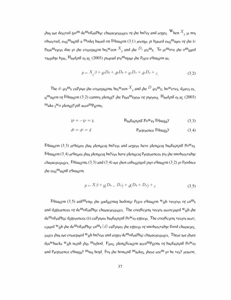
variable bias, Harding et al. (2003) instead formulate the price equation as:

p = X1β + bbDb + dbDb + bsDs + dsDs + ε. (3.2)

The di terms capture the correlations between X2 and the D terms; however, direct es-

timation of Equation (3.2) cannot identify the parameters of interest. Harding et al. (2003)

make two identifying assumptions:

bb = −bs = b Bargaining Power Equality (3.3)

db = ds = d Preference Equality (3.4)

Equation (3.3) requires that identical buyers and sellers have identical bargaining power.

Equation (3.4) requires that identical buyers have identical preferences for the unobservable

characteristics. Equations (3.3) and (3.4) are then substituted into equation (3.2) to produce

the estimating equation:

p = Xβ + b�Db −Ds) + d�Db + Ds) + ε (3.5)

Equation (3.5) augments the traditional hedonic price equation with vectors of sums

and differences of demographic characteristics. The coefficient vector associated with the

demographic differences (b) captures bargaining power effects. The coefficient vector asso-

ciated with the demographic sums �d) captures the effects of unobservable good character-

istics that are correlated with buyers and seller demographic characteristics. There are three

drawbacks with using this method. First, identification assumptions of bargaining power

and preference equality must hold. For the housing market, these seem to be very reason-

37

able identification assumptions. Second, the estimated coefficients can be slightly difficult

to understand and interpret. Finally, the data must have sufficient variation between buyer

and seller demographics in order to estimate the b coefficients with precision.

This model has been frequently used to analyze price formation in real estate. Colwell

and Munneke (2006) apply the model to commercial property noting that the b terms may

be capturing market imperfections while d may reflect different (unobservable) “classes” or

market segments in which types prefer to be active. Ihlanfeldt and Mayock (2009) find that

race is a determinant of sale price of Florida houses. Cotteleer et al. (2008) argue that the

b terms are more properly characterized as “personal characteristics.” They claim that the

preference equality assumption in equation (3.4) is restrictive. Instead of using Equations

(3.3) and (3.4) to identify bi and di, the authors assume that there are no omitted charac-

teristics in their estimating equation that are correlated with both price and demographic

characteristics (db = ds = 0). Therefore, buyer and seller demographics can enter the esti-

mating equation directly. This identification assumption is not econometrically testable.

3.2 The Days­at­Sea Market

There are thirteen species and twenty-four separate stocks of groundfish which are managed

jointly in the Northeast United States. These include both round (cod, haddock) and flat

fish (flounders). Of these stocks, thirteen are classified as overfished and overfishing is

currently occurring in five of the stocks (NMFS, 2008)1. These fish are caught by a diverse

fishing fleet that uses a wide variety of fishing gear (otter trawls, gillnets, and hook-and-

line) and fishing locations. The fishery is a a joint, multiproduct fishery (Squires, 1987;

Kirkley and Strand, 1988). Labor is compensated using the lay or share system; employees

receive a share of total revenue, after deducting variable operating costs (McConnell and

1When a stock of fish is “too small”, it is overfished. When the flow of fish being harvested is “too high”,

overfishing is occurring. Neither an overfished stock nor the occurrence of overfishing necessarily implies

the other.

38

Price, 2006). The exact share percentages and definitons of variable operating costs vary by

vessel. The vessels that participate in the groundfish fishery typically participate in other

fisheries in the Northeast United States, including the scallop, monkfish, lobster, and small

pelagic fisheries. Some of these species are caught jointly with groundfish.

Days-at-Sea (DAS) has been the primary management tool used to reduce fishing effort

directed at groundfish in the Northeast United States2. In 1996, there were approximately

1,700 vessels with an aggregate allocation of approximately 236,000 DAS (Code of Fed-

eral Regulations, title 50, Part 648, 2004). Substantial reductions in DAS were made so

that by 2004, there were 1,400 vessels with a permit to fish 44,000 DAS, although not ev-

ery permitted vessel had a DAS allocation. Leasing has become increasingly important;

by 2008 over 40 percent of all used DAS were leased (Table 3.1). Although input con-

trols have long been known to be an economically inefficient management tool (Wilen,

1979; Townsend, 1985), these management instruments have been popular in the fishing

and fishery management communities (Rossiter and Stead, 2003).

At the beginning of the fishing year (May 1), vessels are allocated a stock of DAS which

may be used at any time during the year. These DAS are similar to call options; a fishing

vessel that owns a Northeast Multispecies DAS has the right to fish for groundfish in the

Northeast United States federal waters for certain period of time during the fishing year.

Up to 10 unused DAS may be carried forward to the subsequent fishing year. Surplus DAS,

beyond ten, expire at the end of the fishing year on April 30 and are worthless. As options,

the value can be decomposed into a time-value component and an intrinsic value compo-

nent. The time-value component should decline to zero as the trade date approaches the end

of the fishing year. DAS differ slightly from traditional options; the intrinsic value of the

option varies across fishing vessels and is based on the fishing technology and other vessel

characteristics. A vessel that chooses to sell DAS believes that the expected value from

fishing is less than market price. A vessel that chooses to buy believes that the expected

2Other regulatory tools in use include daily trip limits for certain species, both permanent and rolling area

closures, and minimum mesh sizes.

39

value from fishing is higher than market price.

Trades may occur at any time except the final month of the fishing year3. Prices and

quantity traded must be reported to the National Marine Fisheries Service4. However,

traded prices and quantities are not publicly available, limiting price discovery process

and possibly affecting the market equilibration process (Anderson, 2004). The primary

restriction on trade is related to fishing power:

A lessor may not lease DAS to any vessel with a baseline horsepower rating

that is 20 percent or more greater than that of the horsepower baseline of the

lessee vessel. A lessor also may not lease DAS to any vessel with a baseline

[length] that is 10 percent or more greater than that of the baseline of the lessee

vessel’s [length] (Code of Federal Regulations, title 50, Part 648).

Larger, more powerful vessels are believed to have higher catch rates, particularly for

mobile gear relative to fixed or hook gear vessels. Furthermore, subleasing of DAS is pro-

hibited. Combined with the size and power restrictions, the subleasing prohibition prevents

“ratcheting,” in which Days-at-Sea are successively transferred from small vessels to large

vessels. However, this may also eliminate speculation and market-making activities, which

are thought to be important for markets to efficiently allocate resources. These two limita-

tions on trade are likely to prevent effort from shifting to larger, more efficient vessels by

segmenting the DAS market in to many smaller sub-markets. Small vessels that desire to

acquire DAS and large vessels that wish to divest DAS have the largest number of potential

trading partners (Table 3.2). These types of firms may be able to exert market power in the

Days-at-Sea market. Conversely, the largest buyers and the smallest sellers have the fewest

number of potential trading partners and may have minimal bargaining power. There are

two additional restrictions on trade which may reduce the ability of the market to efficiently

3These trades are technically leases - DAS are transferred for a single fishing year. While permanent

transfer of DAS is allowed, these are infrequent and are not examined in this essay.4A sample lease reporting form is available at http://www�nero�noaa�gov/permits/forms�

html

40

allocate DAS. An upper limit on the number of DAS that a vessel can acquire was set at a

vessel’s 2001 DAS allocation, which may constrain the maximum number of days fished

by some of the most efficient vessels. Because there is no centralized market, trading part-

ners are found by word-of-mouth, advertisement in fishing-specific newspapers, or through

brokers who match buyers to sellers.

A Day-at-Sea permit initially allowed fishing for a 24- hour period; however, there two

major changes in fishery policy during the 2006 fishing year that changed the definition of

a Day-at-Sea. The New England Fisheries Management Council (NEFMC) desired lower

fishing mortality during the 2006 fishing year. However, the regulatory process could not

be completed by the beginning of the fishing year. For approximately six months of the

fishing year (May 1, 2006 to Nov 21, 2006), management of the the groundfish fishery

proceeded under an Emergency Action. All vessels fishing for groundfish were charged

1.4 DAS for each day that was actually used. This Emergency Action was a temporary

means to reduce fishing effort and harvest while the regulatory process was being finished.

At the beginning of the 2006 fishing year, the exact specifications and effective date of the

new regulations were not known with perfect certainty. However, fishermen probably had

reasonably good predictions based on the extensive public notice given by the NEFMC.

Georgianna et. al ( 2008) found that New Bedford based fishing vessels substituted non-

DAS trips for DAS trips and delayed use of their DAS during the 2006 fishing year, waiting

for a more favorable accounting rate. However, the timing of use at an aggregate level does

not appear to have changed (Figures 3.3 and 3.4).

The permanent change to groundfish policy was titled Framework Adjustment 42 and

published on October 23, 2006 with implementation date of Nov 22, 2006. This regulation

created Differential DAS areas with heterogenous DAS costs (See Figure 3.2). Vessels that

used the Differential DAS areas were charged at a rate of two DAS for each day fished.

Fishing in other zones was charged at the normal rate (one-to-one). While fishing vessels

are mobile and may be able to switch fishing locations, there are limits to that mobility.

41

Small vessels may not have be speed or size required to fish far off-shore, gear may be

suitable to certain fishing areas, and crew many not have the knowledge required to use

unfamiliar fishing areas. The differential DAS regulation contained in Framework Adjust-

ment 42 can be thought of as a downward technological shock to the production function

of fishing vessels that use differential Days-at-Sea areas. Fishing vessels that use the Dif-

ferential Days-at-Sea areas will produce less revenue per DAS while those outside this area

should be unaffected.

3.3 Empirical Model and Data Used

In the present application, the traded good confers the right to fish for a period of time.

Harding et al. (2003) make the assumption that buyer and seller demographics confer

bargaining power equally and that identical types (as measured by demographics) have

identical preferences. These identification assumptions are made because the authors are

concerned about omitted variable bias. A Northeast Multispecies Day-at-Sea has a well-

specified legal definition that is consistent across fishing vessels. Prior to 2006, one DAS

allowed vessels to fish for one day. During the Emergency Action period, 1.6 DAS were

required for one fishing day. After the implementation of Framework 42, a DAS allowed

vessels to fish at a a 1:1 ratio in the normal DAS areas or a 2:1 ratio in the differential

DAS areas. While the legal definition of DAS has change over time and currently varies

according to fishing area, there are no unobserved attributes of a DAS. the ds and db terms

in equation (3.1) must be zero and the assumption of bargaining power equality in equation

(3.3) can be safely relaxed. The price equation can be estimated by OLS as:

pi = bbDbi + bsDs

i + γZ + �i (3.6)

The demographic characteristics of buyers and sellers can enter the price equation di-

rectly and bargaining-power symmetry can be tested econometrically. For demographic

42

Dj , rejection of the hypothesis that bbj = −bs

j can be interpreted as evidence that charac-

teristic Dj confers bargaining power asymmetrically to buyers and sellers. Z is a vector of

controls that are not specific to either buyer or seller that may shift price.

The quantiles are modeled as linear. Let Qτ �p|ZX) quantile of the distribution of Days-

at-Sea price, conditional on X , the buyer and seller demographic characteristics and other

price shifters. The conditional quantiles are modeled as:

Qτ �p|X) = X �βτ (3.7)

For any τ ∈ �0� 1), the coefficient vector β�τ) can be estimated by minimizing

1

n

n�

i=1

ρτ �pi −X �

iβτ )

where

ρτ �u) = u�τ − I�u < 0))

For a given quantile, τ , the ρτ �u) function can be interpreted a function that incorporates

asymmetric weights on the residuals that depend on the sign of those residuals.

OLS focuses on the conditional mean and imposes slope homogeneity - the partial

effect of an independent variable on the dependent variable is assumed to be constant. In

contrast, quantile regression allows the estimated coefficients to vary across the ranking

of the dependent variable (Koenker and Bassett Jr., 1978; Koenker and Hallock, 2001).

Using this method, it is possible to examine bargaining power across the distribution of

DAS prices. The restrictions on trade may have segmented the large market for DAS into

many small ones, each with few participants. Small changes in length or horsepower may

have large effects on bargaining power. The bargaining power effects are likely to be most

pronounced at both tails of the price distributions and quantile regression is able to uncover

those effects.

43

The unit of observation in this analysis is a reported trade of a quantity of Days-at-Sea

that occurred in fishing years 2004-2008. There are 1,788 observations for which DAS were

exchanged at positive prices5. Demographic characteristics for buyers and sellers include

length, horsepower, revenues from DAS and alternative fisheries, number of permits held,

fishing gear used, and the amount of prior experience in this market. In general, vessels

that purchased DAS had higher revenues, more experience in the market, and were more

likely to fish using trawl gear and in the Differential DAS areas than the sellers (Table

3.3). Buyers were slightly shorter in length and had lower horsepower, a expected result

of the trading regulations pertaining to those two characteristics. In general, prices had a

downward intra-year trend with fairly large volatility (See Figure 3.1).

Revenues for DAS trips were aggregated at the yearly level and divided by the total

Days-at-Sea used to construct a per-day measure of revenues for buyers and sellers from

the groundfish fishery. The average revenue per-day, lagged one year, were used in the

estimation as a measure of profitability. The decision to acquire or divest DAS is related

to profitability, this is likely to be very closely related to revenue due to the share system

of labor compensation. The DAS revenue variables captures the trade surplus over which

the two parties bargain over. Because fishing vessels are often active in other fisheries,

two other variables were constructed to account for the opportunity costs of buying and

selling DAS. The first variable directly measures daily revenue from alternative fisheries;

this variable is constructed analogously to the DAS Revenue variable. The second variable

included is the number of other limited access permits held by each vessel. The Alternative

Revenue and Permits variables control for the opportunity costs of fishing and are also

related to the trade surplus. Vessels with high alternative revenues and many limited access

permits have a relatively high opportunity cost using DAS; they have highly productive

alternative fishing activities. All economic data (prices and revenues) was deflated using

5Of the 2,349 observed transactions, 561 transactions reported a price paid equal to zero. There were

an additional 115 transactions for which the price was less than �100. There may represent intra-company

trades, non-response, or indicate a catch-sharing agreement. Additionally, there are a few (n=7) outlying data

points for which the price is far higher that the rest of the sample.

44

Bureau of Labor Statistics Producer Price Index for unprocessed finfish, with the base year

set to 2008.

For each transaction, the buyer’s and seller’s experience is constructed as the number

of times each party had previously participated in the DAS market. The expected effect of

this variable is unclear: frequent participants are likely to have an informational advantage

relative to infrequent participants which may translate to a bargaining power advantage.

However, experience may reflect self-selection into the market; buyers with exceptionally

high profitability may be more likely to purchase DAS at any price. Similarly, sellers with

low productivity may be more likely to sell DAS at any price.

A dummy variable for the use of trawl gear is included in the model. Vessels that

use trawl gear are typically larger, more powerful, and catch more fish than vessels that

use long-line, hand-line, or gillnet gear. This variation is already captured in the variables

used; however, trawl vessels also have higher operating expenses, mostly due to higher

fuel usage. Although detailed variable cost information is not available at the vessel-level,

inclusion of a dummy variable for trawlers may capture the higher variable operating costs

associated with this type of gear.

Two variables are used to capture the possible the effects of the technological shock

imposed by Framework 42’s Differential Days-at-Sea regulations. The fraction of revenues

derived from trips in the differential DAS areas was constructed using locational data from

landings reports (Figure 3.2). This variable captures the relative importance of the Differ-

ential DAS areas for each fishing vessel. A dummy variable was included for trades that

occur after Framework 42 was implemented; this variable is also interacted with the Dif-

ferential DAS fraction. Yearly dummy variables were also included in the estimated model

and based on the fishing year (May-April). The variable “Time Remaining” constructed

from the reported trade date and is used to capture the time-value component of DAS. Ig-

noring carry-over to the next fishing year, the value of unused DAS is zero on the final day

of the fishing year.

45

A linear model is estimated using OLS on the full sample (N=1,788) and two subsam-

ples that drop prices over �3,000 and �1,500 respectively6. The model is then estimated

using the full sample using quantile regression for the 10th through 90th quantiles, at inter-

vals of 5%, using the quantreg package in R.

3.4 Results

The linear model fit by OLS fits moderately well; R2 ranges from 0.21 to 0.51 (Tables

3.4 and 3.5). Results seem to be sensitive to outlying data points. Estimated coefficients

and significance levels, particularly the Trawl Buyer, Permits Seller, Framework42, and

Framework42∗DDAS Buyer, are not stable across subsamples. Furthermore, inspection

of the residuals reveals that the model has some difficulty fitting both the very high and very

low prices (Figure 3.5). These findings partially motivate the use of quantile regression.

Because buyer and seller demographic characteristics enter the estimating equation sep-

arately, it is possible to examine the Bargaining Power equality assumption. Bargaining

Power equality implies that coefficients for buyer and seller demographic characteristics

sum to zero. Table 3.6 contains the linear combination bs + bb and t−statistics for demo-

graphic characteristics. Rejection of the null hypothesis indicates that Bargaining Power

equality does not hold. Postive values in Table 3.6 imply that increases in that characteristic

are associated with increases in DAS price and may be interpreted as increasing the relative

bargaining power of sellers. Negative values are associated with decreases in DAS price

and may be interpreted as increasing the relative bargaining power of buyers.

A major finding is that segmentation induced by the trading restriction on length con-

fers bargaining power unequally to buyers and sellers. The positive combination of coeffi-

cients for length implies that longer buyers have less bargaining power. Although there are

also trading restrictions based on horsepower; neither buyer nor seller power affect DAS

6The specification presented standardize horsepower by dividing by vessel length. The appendix contains

a slightly different analysis that uses raw horsepower and monthly dummy variables.

46

price. A somewhat surprising finding is that revenues-per-DAS have no effect on bargain-

ing power; however, there is moderate evidence that alternative fishing revenue and limited

access permits increase the bargaining power of sellers. Finally, there is weak evidence

that use of the differential DAS areas either reduces the willingness-to-pay for DAS or

decreases the bargaining power of sellers after the implementation of differential DAS.

Utilization of the Differential DAS area by either buyer or seller prior to implemen-

tation of Framework 42 has no statistically significant impact on bargaining power. The

implementation of Framework 42 may have increased price; however this results is not ro-

bust across models7. For the smallest subsample (Model 3), buyers that use the differential

Days-at-Sea will pay less after the implementation of Framework42. Vessels that heavily

utilize the differential DAS areas find those areas less profitable and therefore are willing

to pay less in order to fish there. It is plausible that the trade surplus decreased under

Framework 42, driving down prices.

The Time Remaining coefficient is positive and significant, providing support for the

time-value component of Days-at-Sea valuation. The estimated coefficient is relatively

stable across the three estimated models, ranging from �0.36-0.52 per day. The coefficients

for yearly dummies are presented in Table 3.5. There were substantial price increases

in 2006-2008, relative to 2004. Real DAS prices were up to �200 higher in 2006-2008;

although the estimated coefficients vary by specification and year.

The quantile regression method can provide further insight into the bargaining process

beyond analysis of the conditional mean price. Tables 3.6 and 3.7 contain coefficient es-

timates and standard errors for 5 selected quantiles along with Koenker and Machado’s

(1999) R1 statistic8. The model has little explanatory power at the lower tail of the price

7Based on Model 2, the sum of the F42xDifferential seller and Framework42 coefficients is �77; however,

the standard error of that estimate is 52, indicating that it cannot be statistically distinguished from zero.

Similarly, the sum of F42xDifferential buyer �40, with a standard error of 45, also not distinguishable from

zero.8The R1 is an analog of the R2 statistic and is calculated as R1

= 1 − Vu

V�

, where Vu is the value of the

objective function produced by a “full regression” and Vc is the value of the objective function produced by

regression of price against only a constant.

47

distribution; there is little variation in the dependent variable and prices are clustered just

above zero. Fit improves markedly at higher quantiles. Visualization is the easiest way to

interpret results of quantile regression; each of the estimated coefficients, βτ , are plotted as

a function of τ , along with shaded 90% confidence bands and a dotted line that represents

the OLS coefficient estimate. The graphs and associated coefficients can be interpreted as

the marginal effect of an independent variable on price at a given quantile. A line with

zero slope would be consistent with the slope-homogeneity restriction imposed by least

squares. Departures from zero slope imply that the marginal effects are different across

different price quantiles. Many, but not all of the coefficient lines appear to have non-zero

slope.

These results are consistent with regulatory segmentation hypothesis based on length.

Length reduces the bargaining power of buyers; however, this effect is strongest at the

upper tail of the price distribution and non-existent at the lower tail. An extra foot of

buyer’s length increases the price of DAS by �5.20 at the 25th percentile and by �10 at

the 90th percentile (Figure 3.7). In addition, seller length has a similar, though smaller in

magnitude, effect on prices at the higher price quantiles (Figure 3.8). Power, as measured

by the horsepower/length ratio does not seem to impact the bargaining power of buyers

or sellers (Figures 3.9 and 3.10). Length, and not power, seems to be more restrictive in

determining feasible trades in this market.

Groundfish revenues for both buyer and seller are related to the trade surplus over which

each party bargains. Buyer’s groundfish revenue appears to have no effect on prices while

seller’s groundfish revenues have a small effect, increasing price by approximately �7 per

�1,000 of daily revenues at all but the lowest price quantiles (Figures 3.11 and 3.12). The

effects of the alternative revenue and limited access permits are similar: conferring small

amounts of bargaining power to sellers at the low and moderate price quantiles (Figures

3.13 and 3.14) and having no effect on the bargaining power of buyers (Figures 3.15 and

3.16). These findings could indicate a gradient of market classes. There may be one market

48

class for the large vessels; in this segment, size is an important determinant of price and

bargaining power. There is another market class for the smaller vessels; within this class,

the profits and opportunity costs of the seller, as measured by Permits, DAS Revenue, and

Alternative Revenue become more important in the bargaining process.

Implementation of Framework 42’s Differential DAS system had an interesting effect

on prices and bargaining power. As expected, prior to the implementation of Framework

42, the bargaining power of vessels that used the Differential DAS areas did not system-

atically vary from vessels that did not use these areas (Figures 3.17 and 3.18). The signs

and significance of the Framework42, Differential DAS, and interaction variables were not

robust in the OLS model. The quantile regression results suggests that is due to fairly sub-

stantial heterogeneity in the effect of these variables. After implementation of Framework

42, the prices in the lower quantiles were unchanged or slightly lower; however, prices at

the middle and higher quantiles increased substantially, by �80-150 (Figure 3.19). How-

ever, there is an additional effect due the interaction of the Framework 42 and Differential

DAS variables. Table 3.8 further examines the effects of Framework 42 when the buyer,

seller, both, or neither use the Differential DAS areas. In general, prices after Framework

42 remained constant if the buyer exclusively used the Differential DAS areas. If the buyer

did not use those areas, prices were sustantially higher.

The yearly price effects estimated by quantile regression are similar to the effects esti-

mated by OLS. Relative to 2004, all prices were higher in 2006. However, prices in 2007

and 2008 were only higher in the middle quantiles of the price distribution (Figure 3.23).

Higher prices in 2006 could reflect some of the regulatory uncertainty regarding the Emer-

gency Action and the timing of the adoption of Framework 42. The large coefficient on the

2006 dummy variable reflects higher prices during the time in the fishery operated under

the 1.4-to-1 DAS counting mandated by the Emergency Action. Also consistent with the

OLS results, trades that occur later in the year occur at lower prices (Figure 3.22). Con-

sistent with the interpretation of DAS as options; the value of a DAS decays at the rate of

49

approximately �0.50 per day across most of the price quantiles.

It is also possible to examine bargaining power at individual quantiles. Table 3.9 con-

tains the sums of buyer and seller demographic coefficients (bs + bb) and t−statistics for

demographic characteristics at 5 selected quantiles. A positive combination indicates that

increases in the independent variable lead to higher price. This may be evidence that the

independant variable confers bargaining power to sellers. Conversely, a negative combina-

tion indicates that increases in the dependent variable leads to lower prices. This may be

evidence that the independent variable confers bargaining power to buyers.

In general, there is substantial heterogeneity in the net effect of buyer and seller char-

acteristics across quantiles. Sums of coefficients are generally insignificant at the τ = 0.10

quantile. These results strongly reject the hypothesis that length confers bargaining power

equally to buyers and sellers at the 50th percentile and higher; length lowers the bargaining

power of buyers relative to sellers. This effect seems to be slightly larger at the higher price

quantiles. The bargaining effects of power are not robust across quantiles. There is also

very weak evidence that higher groundfish revenues confer bargaining power to sellers in

the middle price quantiles. The two measures of opportunity costs of using DAS are also

non-robust across quantiles. Permits have a fairly large positive effect on seller’s bargain-

ing power, but this only occurs at the 25th percentile of price. At this price level, alternative

revenue have a small negative effect on seller bargaining power; while at the 50th percentile

alternative revenue has a small positive effect on seller bargaining power.

Trawl usage may confer bargaining power to buyers at the middle quantiles of price.

However, this finding is also consistent with higher costs and therefore lower willingness-

to-pay for buyers that use trawl gear. Usage of the Differential DAS areas has a fairly large

negative effect on seller bargaining power at the higher price quantiles, although this effect

reverses itself and disappears at the lower price levels. Again, these findings are consistent

with lower productivity of DAS under the Differential DAS managment regime and may

not be directly indicative of changes in bargaining power.

50

3.5 Conclusions

This chapter expands on the Harding et al.’s (2003) model in two ways. First, by ex-

amining a good without unobserved characteristics, the assumption of bargaining power

equality used for identification can be econometrically tested. Based on analysis using

least squares, the hypothesis of bargaining power equality can be rejected for some de-

mographic characteristics, most notably vessel length. Secondly, this research applies an

alternative econometric technique, quantile regression, to examine the effects of bargaining

power. This method allows for the effects of demographic characteristics on price to vary

across the price distribution.

The major finding of this research is the trading restrictions based on size and power led

to unequal bargaining power for buyers and sellers. This finding can resolve an apparent

inconsistency in this market; DAS trade at positive prices even though, in aggregate, there

is excess supply of DAS (as measured by unused DAS). The size and power trading re-

strictions appear to have segmented the DAS market so that there is only excess supply for

smaller, less powerful vessels. A well-designed market for an input permit can efficiently

allocate those permits to the most efficient firms. In this market, limitations on trade have

conferred market power to certain types of individuals.

The productivity of DAS (revenues) do not affect the bargaining power to either buyers

or sellers. This surprising finding may occur because the restrictive size and power regula-

tions dominate bargaining power changes of revenues. Alternatively, the revenue variable

used may be a poor measure of firm-level profitability. The share (or lay) system of labor

compensation is used in this fishery; crew are typically paid a fraction of total revenues

minus variable costs and the owner of the fishing vessel receives a share of total revenues.

Therefore, the returns to the owner from using a DAS should be reasonably correlated to

51

revenues although heterogeneity in the shares system may limit the ability of revenue to

control for firm-level profitability.

The negative relationship between price and Time Remaining is likely related to decay

in the time-value of the option. However, alternative interpretations are possible, although

less likely. Sellers could lose bargaining power relative to buyers during the year. How-

ever, a reason for decreases in bargaining power is not clear. Furthermore, the timing of

purchases matters because a vessel cannot hold a negative amount of DAS. If a vessel

runs out of DAS, it must stop fishing unless it can acquire DAS. This may explain higher

willingness-to-pay for DAS early in the fishing year.

These results have implications for fisheries management and general design of mar-

kets. Fishery managers were likely concerned with an increase in total catch associated

with transferring DAS from small vessels to larger, more-efficient vessels. The trading

restrictions based on size and power designed to limit expansion of effort appear to have

segmented the market, inflating the prices paid by largest buyers relative to vessels of other

sizes and depressing the prices received by smaller vessels. Ensuring the continued opera-

tion of a diverse fishing fleet was a goal of managers; while the strict regulations on trade

may have accomplished that goal, the cost of this regulation is lower bargaining power for

the smaller fishing vessels.

52

3.6 Tables and Figures

Allocated Used Aggregate Aggregate Value

Year DASa DAS Leased DAS of Leased DAS

2004 44,030 30,060 6,192 � 2,590,182

2005 51,112 32,194 8,068 � 2,709,263

2006 48,175 32,399 11,245 � 3,279,149

2007 47,802 33,264 13,900 � 4,815,603

2008 47,021 31,701 13,996 � 4,494,270a:Includes DAS carried over from previous fishing year.

Table 3.1: Historical Days-at-Sea Allocations, Usage, and Leases. Extracted from NMFS

DAS and DAS2 databases.

Length Potential Buyers Potential Sellers

30 feet 924 132

40 feet 810 540

53 feet 517 816

70 feet 318 1,069

80 feet 209 1,204

100 feet 33 1,263

Table 3.2: Number of feasible trading partners by length.

53

0200

400

600

800

1000

Price (2008 $)

01500

Volume

2004m1 2005m1 2006m1 2007m1 2008m1 2009m1Date

Figure 3.1: Median and Interquartile range of real DAS prices, Monthly DAS volume

54

������

����������������������� �� �� �� ���

�����

Figure 3.2: The Differential DAS areas were implemented with Framework Adjustment 42

on Nov 22, 2006.

55

1500

2000

2500

3000

3500

4000

DAS Used

1 12Month

2004 2005 2006 2007 2008

Figure 3.3: Monthly DAS Usage.

200

400

600

800

1000

1200

DAS Used

0 10 20 30 40 50Week

2004 2005 2006 2007 2008

Figure 3.4: Weekly DAS Usage.

56

Buyer

Sel

ler

Var

iable

Defi

nitio

nM

ean

Std

.D

evM

ean

Std

.D

ev

Price

Price

per

DA

Sin

2008

Dollar

s�360

521

Quan

tity

Day

strad

ed22.3

15.3

Len

gth

Ves

selle

ngth

infe

et60.2

19.1

62.3

18.9

Hors

epow

erVes

selH

ors

epow

erR

atin

g437

190

504

241

Pow

erH

ors

epow

er/L

ength

7.2

01.7

88.0

42.5

6

DA

SR

even

ue

per

DA

S,000sofdollar

sper

day

�3.9

23.1

3�1.0

32.3

9

Alter

nat

ive

Rev

enue

per

Day

Fis

hed

,no

DA

Suse

d,000sofdollar

sper

day

�1.9

33.2

0�1.8

24.2

1

Per

mits

Num

ber

oflim

ited

acce

ssper

mits

2.3

51.5

91.4

61.9

9

Exper

ience

Num

ber

oftim

esa

ves

selhas

trad

edin

the

DA

Sm

arket

4.5

4.5

2.5

2.5

Tra

wl

Dum

my

var

iable

=1

ifves

seluse

straw

lgea

r,=0

oth

erw

ise

0.6

90.4

60.8

00.4

0

Diffe

rential

Fra

ctio

nofre

ven

ues

from

diffe

rential

DA

Sar

eas

0.4

58

0.4

39

0.1

49

0.3

32

Tim

eR

emai

nin

gN

um

ber

ofD

aysre

mai

nin

gin

Fis

hin

gYea

r171

95.6

Tab

le3.3

:Sum

mar

ySta

tist

ics

(N=1,7

88):

Eco

nom

icvar

iable

snorm

aliz

edto

2008

real

val

ues

usi

ng

Pro

duce

rPrice

Index

forU

npro

-

cess

edFin

fish

.B

uyer

and

seller

mea

ns,

exce

ptA

lter

nat

ive

Rev

enue,

are

stat

istica

lly

diffe

rentat

the

1%

level

.

57

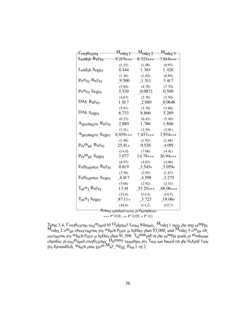
Coefficient Model 1 Model 2 Model 3

Length Buyer 9.219*** 8.723*** 7.610***

(1.25) (1.08) (0.93)

Length Seller 0.444 1.363 1.420

(1.36) (1.02) (0.89)

Power Buyer -9.500 -1.511 3.417

(5.84) (4.78) (3.70)

Power Seller 5.539 -0.0972 0.509

(4.67) (2.78) (2.50)

DAS Buyer 1.017 -2.880 -0.0648

(5.07) (3.70) (3.06)

DAS Seller 6.733 8.866 5.269

(6.23) (6.43) (5.49)

Alternative Buyer 2.880 1.786 1.866

(3.21) (2.59) (2.01)

Alternative Seller 8.039*** 7.437*** 7.934***

(1.96) (1.92) (1.68)

Permits Buyer 25.41* 0.536 -4.091

(14.0) (7.06) (4.41)

Permits Seller 7.077 14.79*** 26.94***

(6.97) (4.83) (4.06)

Experience Buyer 0.619 -3.545* -3.059*

(3.58) (2.05) (1.67)

Experience Seller -4.417 -4.598 -3.275

(5.66) (2.92) (2.53)

Trawl Buyer 13.41 -53.25*** -68.06***

(33.6) (14.4) (10.5)

Trawl Seller -87.11* -3.723 -18.06*

(44.6) (14.2) (10.7)

Robust standard errors in parentheses

*** p<0.01, ** p<0.05, * p<0.1

Table 3.4: Coefficients estimated by Ordinary Least Squares. Model 1 uses the full sample,

Model 2 omits observations for which price is higher than �3,000, and Model 3 omits ob-

servations for which price is higher than �1,500. Trimming of the sample leads to moderate

changes in estimated coefficients. Dummy variables for Year are based on the fishing year

for groundfish, which runs from May-April. Part 1 of 2.

58

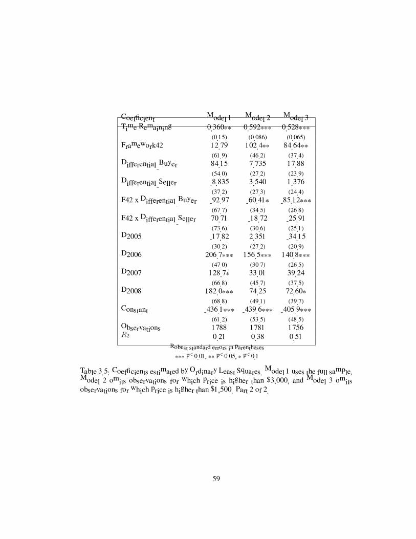
Coefficient Model 1 Model 2 Model 3

Time Remaining 0.360** 0.592*** 0.528***

(0.15) (0.086) (0.065)

Framework42 12.79 102.4** 84.64**

(61.9) (46.2) (37.4)

Differential Buyer 84.15 7.735 17.88

(54.0) (27.2) (23.9)

Differential Seller -8.835 3.540 1.376

(37.2) (27.3) (24.4)

F42 x Differential Buyer -92.97 -60.41* -85.12***

(67.7) (34.5) (26.8)

F42 x Differential Seller 70.71 -18.72 -25.91

(73.6) (30.6) (25.1)

D2005 -17.82 2.351 -34.15

(30.2) (27.2) (20.9)

D2006 206.7*** 156.5*** 140.8***

(47.0) (30.7) (26.5)

D2007 128.7* 33.01 39.24

(66.8) (45.7) (37.5)

D2008 182.0*** 74.25 72.60*

(68.8) (49.1) (39.7)

Constant -436.1*** -439.6*** -405.9***

(61.2) (53.5) (48.5)

Observations 1788 1781 1756

R2 0.21 0.38 0.51

Robust standard errors in parentheses

*** p<0.01, ** p<0.05, * p<0.1

Table 3.5: Coefficients estimated by Ordinary Least Squares. Model 1 uses the full sample,

Model 2 omits observations for which price is higher than �3,000, and Model 3 omits

observations for which price is higher than �1,500. Part 2 of 2.

59

−2000

02000

4000

6000

8000

Residuals

−500 0 500 1000 1500Fitted values

Figure 3.5: Residuals vs. Fitted values, Model 1. While most residuals are fairly small,

there are a good number observations for which predicted prices were low but actual prices

were high.

60

(1) (2) (3)

Length 9.66 10.10 9.03

(9.09) (11.58) (14.53)

Power -3.96 -1.61 3.93

(-0.72) (-0.37) (1.21)

DAS 7.75 5.99 5.20

(0.94) (0.80) (0.83)

Alternative 10.90 9.22 9.80

(2.66) (2.62) (3.89)

Permits 32.50 15.30 22.90

(2.43) (2.03) (4.29)

Experience -3.80 -8.14 -6.33

(-0.66) (-2.39) (-2.13)

Trawl -73.70 -57.00 -86.10

(-2.75) (-3.00) (-6.00)

Differential 75.30 11.30 19.26

(1.65) (0.33) (0.69)

F42xDifferential -22.30 -79.10 -111.00

(-0.25) (-1.96) (-3.47)

Figure 3.6: Sums of buyer and seller demographic coefficients with t− ratios for H0: bb +

bs = 0 in parentheses.

61

Coefficient 0.10 0.25 0.50 0.75 0.90

Length Buyer 0.667� 0�674)

5.199� 0�941)

7.922� 0�799)

9.649� 0�923)

10.050� 1�400)

Length Seller − 0.186� 0�421)

− 2.150� 0�700)

2.103� 0�863)

2.815� 0�870)

4.390� 1�366)

Power Buyer 0.130� 1�315)

− 0.777� 2�608)

4.867� 2�978)

5.728� 2�912)

0.585� 4�104)

Power Seller − 0.417� 1�075)

− 1.109� 1�637)

0.181� 2�273)

2.067� 2�425)

4.779� 3�999)

DAS Buyer − 1.592� 2�275)

− 4.240� 2�987)

6.007� 2�902)

1.657� 2�927)

− 1.052� 4�248)

DAS Seller − 1.528� 4�461)

8.208� 6�085)

7.314� 2�598)

12.151� 4�154)

10.087� 4�884)

Alternative Buyer 0.367� 1�040)

0.172� 2�284)

1.584� 1�987)

1.323� 2�173)

− 0.869� 2�451)

Alternative Seller 5.245� 5�438)

15.179� 2�641)

8.551� 1�865)

4.545� 1�315)

1.050� 2�071)

Permits Buyer − 0.125� 1�557)

− 2.373� 3�662)

− 13.068� 4�180)

− 2.528� 5�004)

9.833� 8�198)

Permits Seller 9.263� 7�579)

41.311� 4�647)

15.096� 3�710)

3.518� 3�791)

− 9.053� 5�919)

Experience Buyer − 0.556� 0�736)

− 2.065� 1�277)

− 3.002� 1�372)

− 1.014� 1�535)

− 3.123� 1�684)

Experience Seller − 0.752� 1�013)

− 3.645� 1�861)

− 0.311� 1�899)

− 1.630� 2�325)

0.375� 3�025)

Trawl Buyer − 8.604� 9�579)

− 52.179� 11�213)

− 52.038� 11�086)

− 43.986� 12�307)

− 1.131� 18�000)

Trawl Seller 3.249� 5�789)

9.677� 13�039)

− 32.638� 12�176)

− 7.800� 10�301)

6.117� 14�074)

Table 3.6: Quantile Regression coefficients for selected quantiles. Standard errors in paren-

theses, generated using 20,000 bootstrap replications. Part 1 of 2.

62

Covariates 0.10 0.25 0.50 0.75 0.90

Differential Buyer 0.397� 9�725)

1.594� 25�413)

17.511� 22�884)

− 3.032� 22�834)

39.947� 32�264)

Differential Seller − 17.131� 33�098)

14.084� 32�045)

5.103� 21�190)

24.513� 21�992)

16.597� 29�168)

F42xDifferential Buyer 12.593� 13�019)

− 8.434� 28�892)

−126.417� 26�750)

−112.816� 27�407)

−135.419� 40�827)

F42xDifferential Seller 5.948� 33�090)

− 37.435� 31�792)

13.272� 26�175)

− 27.688� 24�822)

− 25.748� 36�810)

Framework42 − 7.724� 11�626)

− 14.435� 48�910)

80.510� 37�454)

155.838� 39�940)

156.209� 46�290)

Time Remaining − 0.001� 0�024)

0.265� 0�077)

0.460� 0�062)

0.421� 0�056)

0.485� 0�083)

D2005 − 4.280� 9�205)

− 28.047� 18�378)

− 15.203� 21�566)

− 15.065� 18�928)

− 5.681� 26�049)

D2006 0.989� 8�075)

73.089� 43�789)

162.121� 24�739)

190.622� 25�992)

235.257� 41�658)

D2007 4.093� 12�236)

92.762� 46�744)

102.670� 38�664)

10.803� 40�789)

13.752� 51�254)

D2008 10.460� 15�353)

102.200� 47�997)

117.070� 39�598)

30.039� 41�915)

35.930� 53�385)

Constant − 12.181� 19�915)

−129.895� 54�597)

−451.113� 48�248)

−511.274� 38�782)

−567.143� 50�622)

R1 0.02 0.17 0.41 0.51 0.47

Table 3.7: Quantile Regression coefficients for selected quantiles. Standard errors in paren-

theses, generated using 20,000 bootstrap replications. Part 2 of 2.

63

0.2 0.4 0.6 0.8

02

46

810

12

 

quantile

coefficient

Figure 3.7: Quantile Regression Coefficients - Buyer Length.

0.2 0.4 0.6 0.8

−2

02

46

 

quantile

coefficient

Figure 3.8: Quantile Regression Coefficients - Seller Length.

64

0.2 0.4 0.6 0.8

−10

−5

05

10

 

quantile

coefficient

Figure 3.9: Quantile Regression Coefficients - Buyer Power.

0.2 0.4 0.6 0.8

−5

05

10

 

quantile

coefficient

Figure 3.10: Quantile Regression Coefficients - Seller Power.

65

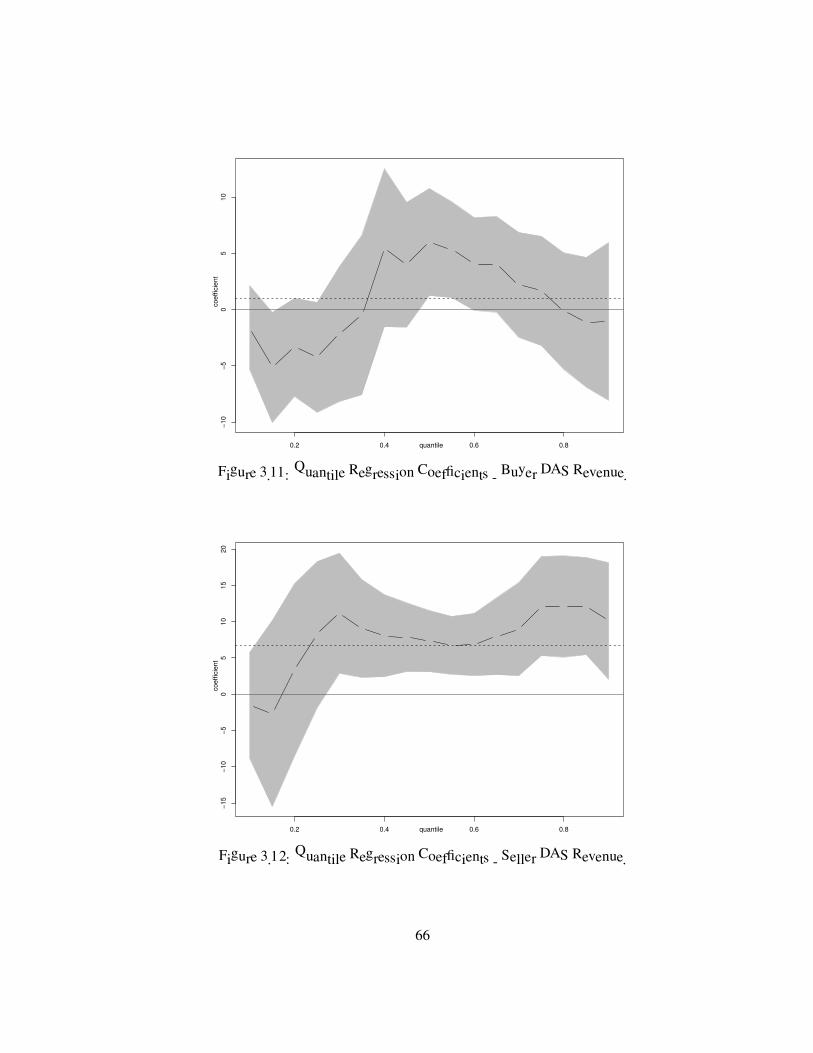
0.2 0.4 0.6 0.8

−10

−5

05

10

 

quantile

coefficient

Figure 3.11: Quantile Regression Coefficients - Buyer DAS Revenue.

0.2 0.4 0.6 0.8

−15

−10

−5

05

10

15

20

 

quantile

coefficient

Figure 3.12: Quantile Regression Coefficients - Seller DAS Revenue.

66

0.2 0.4 0.6 0.8

05

10

15

20

25

 

quantile

coefficient

Figure 3.13: Quantile Regression Coefficients - Seller Alternative Revenue.

0.2 0.4 0.6 0.8

−20

−10

010

20

30

40

50

 

quantile

coefficient

Figure 3.14: Quantile Regression Coefficients - Seller Permits.

67

0.2 0.4 0.6 0.8

−4

−2

02

46

 

quantile

coefficient

Figure 3.15: Quantile Regression Coefficients - Buyer Alternative Revenue.

0.2 0.4 0.6 0.8

−20

−10

010

20

 

quantile

coefficient

Figure 3.16: Quantile Regression Coefficients - Buyer Permits.

68

0.2 0.4 0.6 0.8

−40

−20

020

40

60

80

 

quantile

coefficient

Figure 3.17: Quantile Regression Coefficients - Buyer Differential DAS.

0.2 0.4 0.6 0.8

−50

050

 

quantile

coefficient

Figure 3.18: Quantile Regression Coefficients - Seller Differential DAS.

69

0.2 0.4 0.6 0.8

−100

0100

200

 

quantile

coefficient

Figure 3.19: Quantile Regression Coefficients -Framework 42.

70

0.2 0.4 0.6 0.8

−200

−150

−100

−50

050

 

quantile

coefficient

Figure 3.20: Quantile Regression Coefficients - Buyer F42xDifferential DAS.

0.2 0.4 0.6 0.8

−100

−50

050

 

quantile

coefficient

Figure 3.21: Quantile Regression Coefficients - Seller F42xDifferential DAS.

71

0.2 0.4 0.6 0.8

0.0

0.1

0.2

0.3

0.4

0.5

0.6

 

quantile

coefficient

Figure 3.22: Quantile Regression Coefficients - Time Remaining in Fishing Year.

72

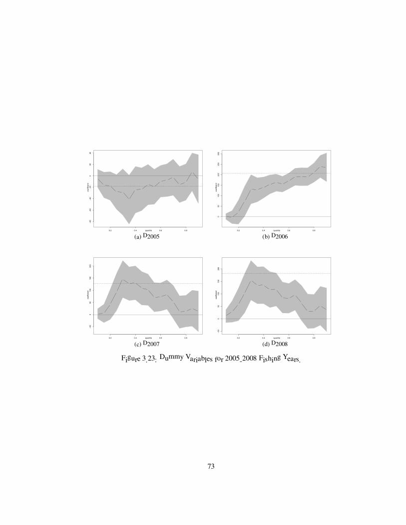
0.2 0.4 0.6 0.8

−80

−60

−40

−20

020

40

 

quantile

coefficient

(a) D2005

0.2 0.4 0.6 0.8

050

100

150

200

250

300

 

quantile

coefficient

(b) D2006

0.2 0.4 0.6 0.8

−50

050

100

150

200

 

quantile

coefficient

(c) D2007

0.2 0.4 0.6 0.8

−50

050

100

150

200

 

quantile

coefficient

(d) D2008

Figure 3.23: Dummy Variables for 2005-2008 Fishing Years.

73

Differential Seller=1 Differential Seller=0

Differential Buyer=1 -60.3 -22.87

(-1.40) (-0.49)

Differential Buyer=0 -51.87 -14.43

(-1.04) (-0.30)

(a) 25th Quantile

Differential Seller=1 Differential Seller=0

Differential Buyer=1 -32.64 -45.91

(-0.88) (-1.26)

Differential Buyer=0 93.78 80.51

(2.21) (2.15)

(b) 50th Quantile

Differential Seller=1 Differential Seller=0

Differential Buyer=1 15.33 43.02

(0.38) (1.06)

Differential Buyer=0 128.15 155.84

(2.87) (3.91)

(c) 75th Quantile

Differential Seller=1 Differential Seller=0

Differential Buyer=1 -4.96 20.79

(-0.09) (0.37)

Differential Buyer=0 130.46 156.21

(2.31) (3.39)

(d) 90th Quantile

Table 3.8: Partial Effect of Framework 42’s Differential Days-at-Sea, for combinations of

Differential Days-at-Sea users (t-statistics in parentheses).

74

0.1 0.25 0.5 0.75 0.9

Length 0.48 3.05 10.03 12.46 14.44

(1.12) (3.85) (13.05) (19.31) (14.14)

Power -0.29 -1.89 5.05 7.80 5.36

(-0.22) (-0.74) (1.89) (3.22) (1.68)

DAS -3.12 3.97 13.32 13.81 9.04

(-0.62) (0.66) (3.57) (2.69) (1.40)

Alternative 5.61 15.35 10.14 5.87 0.18

(1.08) (4.33) (3.73) (2.35) (0.06)

Differential -16.73 15.68 22.61 21.48 56.54

(0.53) (0.44) (0.86) (0.78) (1.46)

Experience -1.31 -5.71 -3.31 -2.64 -2.75

(-1.08) (-2.43) (-1.50) (-0.98) (-0.91)

Trawl -5.35 -42.50 -84.68 -51.79 4.99

(-0.59) (-2.60) (-5.45) (-3.64) (0.24)

Permits 9.14 38.94 2.03 0.99 0.78

(1.22) (6.73) (0.38) (0.18) (0.08)

F42xDifferential 18.54 45.87 -113.15 -140.50 -161.17

(0.60) (-1.20) (-3.41) (-4.60) (-3.46)

Table 3.9: Sums of buyer and seller demographic coefficients with t− ratios for H0: bb +bs = 0 in parentheses.

75

Chapter 4

Economic Tradeoffs in the Gulf of Maine

Ecosystem: Herring and Watching

4.1 Introduction

In contrast to traditional fisheries management which has historically focused on the extrac-

tive fishing industry, Ecosystem Based Fisheries Management (EBFM) prioritizes overall

ecosystem health and attempts to consider all users of ecosystem resources in the decision-

making calculus (Link, 2002; Pikitch et al., 2004). This research examines the effect

of a recent change in fisheries policy, a seasonal ban on trawling for herring in the in-

shore Gulf of Maine, on the commercial whale-watching industry. Drawing upon Crocker

and Tschirhart’s (1992) ecosystem-externality model and Sanchirico and Wilen’s (1999)

spatially-explicit fishery model, this research examines the theory of localized depletion as

it affects the commercial whale-watching industry.

This theory claims that intense trawling for herring causes temporary reductions the

their abundance, depressing the abundances of whales and other highly mobile predators

of herring (Schreiber, 2005; Moser, 2007; Herring Alliance, 2008). If true, this is likely

to lead to increased search times by whale-watching vessels. Extensive search by whale-

watching vessels is costly for firms and is also likely to reduce consumer welfare. Time

spent viewing whales is a “good” while time spent searching is likely to be a “bad.” While

an extensive consumer valuation literature exists for whales (Hoagland and Meeks, 2000;

Loomis et al., 2000; Shaikh and Larson, 2003), this research examines the value of leaving

a stock of fish in the ecosystem.

This research is the inverse of Flaaten and Stollery’s (1996) model, which examined

76

the costs imposed by predatory whales on a fishery. It also related to a large bioeconomic

literature which seeks to understand economically efficient harvest levels in a predator-prey

system (Hannesson, 1983; Strobele and Wacker, 1995; Brown et al., 2005; Hoekstra and

van den Bergh, 2005). In this ecosystem, the spatial location of predators and prey is of

vital importance: whale-watching firms depend on a high abundance of whales that are

close to shore.

4.2 Background

4.2.1 The Whale­watching Industry

Whale-watching is a �30M industry (revenue/year) in New England with approximately

one million commercial passengers and is growing at roughly 10% per year (Hoyt, 2001).

In addition, consumer surplus from commercial trips has been estimated at roughly �29

per trip in the Stellwagen Bank National Marine Sanctuary (Hoagland and Meeks, 2000).

However, no research exists that examines the cost (or value) of the search process from a

consumer point of view. While consumers may view search as a “good”, a “bad”, or both,

firms undoubtedly view increases in search time as an additional cost. The whale-watching

season runs from late spring through early fall, overlapping with a large portion of the

herring fishing season.

Fin, humpback, and minke whales are most commonly sighted on whale-watching trips.

These animals are thought to have fairly strong site fidelity at both large and small scales;

they consistently use the Gulf of Maine to feed on herring, sand lance, and other small

fish (Overholtz et al., 2000; Read and Brownstein, 2003; Robbins, 2007). Despite this site

fidelity, whales are known to be responsive to changes in prey availability (Weinrich et al.,

1997, 2005).

The commercial whale-watching vessels are based in many ports in the Gulf of Maine,

ranging from Provincetown, Massachusetts to Bar Harbor, Maine (Figure 4.1). Fixed costs

77

(physical capital, insurance, wharfage, and crew labor) are high relative to variable costs

(fuel). Higher fuel costs due to increased search time are likely to be the largest short-run

impact of localized depletion. Most whale-watching companies have a home searching area

that is limited by the speed of their vessel and their proximity to oceanographic features

with which whales are commonly associated. A whale-watching trip is advertised to last

between 3 to 4 hours; however, a large portion that time is spent in search and travel.

Vessels depart from port and travel towards a whale-watching area. While whales can

be seen at any time, they are typically found close to the large oceanographic features,

where prey aggregate in large numbers. Because the whale-watching industry is limited

to a relatively small part of the Gulf of Maine, decreased abundance of whales in this area

could impact this industry even if whale populations remain stable across the entire Gulf of

Maine.

In this chapter, the determinants of search time of five of the seven whale-watching

companies located between Gloucester, MA and Rye, NH are examined. The whale-

watching companies analyzed in this study overlap spatially with the southernmost portion

of the herring fishing grounds. These vessels typically travel to the two large oceanographic

features located in this area: the shallow, sandy-bottomed Stellwagen Bank and the some-

what deeper, rocky-bottomed Jeffrey’s Ledge. In this region, herring fishing occurs fairly

often on Jeffrey’s Ledge and very infrequently on Stellwagen Bank.

4.2.2 The Herring Fishery

In the Gulf of Maine, herring are prey for many species of marine life (Overholtz et al.,

2000; Read and Brownstein, 2003; Chase, 2002) and are also target of a �9-20M fishery

(NMFS, pers. comm.) The fishery is primarily pursued with purse seine and mid-water

trawl gear. The herring fishery is a limited-access fishery that is divided into four zones

and managed with a zonal Total Allowable Catch (TAC). The aggregate TAC for herring

are based on a set of reference points that are designed to ensure that fishing occurs at Op-

78

timal Yield (OY), which is set at Maximum Sustainable Yield (MSY) less an allowance for

uncertainty and socioeconomic considerations. The herring stock is currently classified as

underutilized; the industry does not catch the entire aggregate TAC. However, this classifi-

cation is based on traditional single-species management, which does not consider use by

non-human consumers such as whales or predatory fish, or the impacts of herring fishing on

whale-watching. Fishing in the inshore Gulf of Maine (Zone 1A) is most active during the

summer months, spatially and temporally overlapping the whale-watching industry (Figure

4.2).

In addition to a zonal TAC, the inshore fishery is subject to seasonal closures to protect

spawning herring. This closure is designed to ensure reproductive success of spawning

fish. When spawning, herring aggregate into large numbers in the shallow, nearshore areas.

In the southern Gulf of Maine, this closure occurs from mid-September to mid-October.

4.3 Modeling Approach

Localized depletion is thought to be a fundamentally short-term and spatially dependent;

the effects of this phenomenonon are modeled as an ecosystem externality in the spirit

of Crocker and Tschirhart (1992). In this model, there is a (known) relationship between

predator and prey in the ecosystem. The actions of one group of users (fishers) will affect

the welfare of the other group of users (whale-watchers) through the ecosystem processes

that govern the two species. The localized depletion hypothesis requires two processes to

occur: a biological depletion effect on herring and a migration response by whales. As

Crocker and Tschirhart (1992) note, the exact relationships between the predator and prey

are often unknown; however, the impact on human activities is of primary concern, not the

exact workings of the biological system.

Furthermore, the localized depletion hypothesis is concerned with the fine-scale spatial

characteristics of the system. Because whale-watching vessels are confined to the nearshore

79

area by speed and time constraints, whales located in the offshore areas cannot be utilized

by whale-watching firms. Sanchirico and Wilen’s (1999) spatial bioeconomic model pro-

vides a useful framework in which to understand the spatial considerations of the herring-,

whale-, and whale-watching interactions.

The search behavior of whale-watching vessels is assumed to be simple. Whale-watching

vessels leave port in search of whales, traveling at high speeds towards the areas where

whales are likely to be seen. Vessels stop traveling when a whale is sighted and view

the whale(s) for an extended period of time. When this occurs, a trip is considered to be

completed and successful. Not all whale-watching trips are successful; after an extended

period of unsuccessful search, whale-watching vessels may return to port without sighting

a whale.

We assume that whale-watching firms minimize expected search time conditional on

the availability of whales in the searchable area of the ecosystem.

min SearchT imeit�WhalesNt) (4.1)

s.t.WhalesNt = f�HerringNt)

Subscripts i, t, and N refer to individuals, time periods, and nearshore whale-watching

zones respectively. While the actual search time is observable; the choice variables, such

as search direction, speed, or labor devoted to searching, are unobservable. However, the

SearchT ime function is decreasing in whale availability; the existence of large numbers

of whales in the nearshore area leads to low search times for whale-watching vessels. The

localized depletion hypothesis maintains that the availability of whales in the nearshore

area is an increasing function of herring in the search area. Whales may move from areas

of low prey availability to areas of high prey availability.

The actions of the fishing industry are not modeled in this research; however, it is

useful to consider the industry’s objectives. We assume that vessels in this industry are

80

profit-maximizing entities, choosing both when and where to fish based on profitability.

The assumptions that fishers prefer times and areas that have high expected revenues and

low expected costs are at the common to the recent economic efforts to model the spa-

tial behavior of fishing vessels (Bockstael and Opaluch, 1983; Holland and Sutinen, 2000;

Hicks and Schnier, 2008). The catch data generally supports these ideas; catch in the in-

shore zone is high relative to catch in the offshore regions 1. All things being equal, fishing

in the inshore area is preferable due to both lower costs of access and faster round trip

steaming times. Indirectly, location and amounts of fishing can provide some insight into

the availability of herring: fishing activity may be an indicator of high herring availability.

When unregulated, fishing vessels prefer to fish in the inshore area and will not take into

account the depletive effects of their fishing on the whale-watching industry. This is the

(potential) source of the ecosystem externality; and the quantifying this effect is necessary

to successfully implement Ecosystem Based Fisheries Management.

4.4 Data and Econometric Model

In this analysis, three sources of data are used: five whale-watching organizations in the

southern part of the Gulf of Maine provided trip-level data, fishing effort and catch data

were extracted from the NMFS Vessel Monitoring System (VMS) and Vessel Trip Report

(VTR) datasets, and oceanographic data were obtained from the Gulf of Maine Oceano-

graphic Observation System (GoMOOS).

The dependent variable in this study is amount of time, in minutes, that a whale-

watching vessel spends searching for a whale (Search Time). It is constructed from whale-

watching trip reports that are maintained by whale-watching companies and their affiliated

research groups2. These data span the 2002-2006 whale-watching seasons for Gloucester

1http://www�nefmc�org/herring/safe_reports/herringsafe�html2While whale-watching companies typically undertake multiple trips per day, only the first trip of the day

is used in this analysis. The reliability of the dependent variable for subsequent trips is poor.

81

based vessels and the 2003-2006 seasons for New Hampshire and northern Massachusetts

based vessels. During this period, none of the vessels made capital improvements that

would substantially affect their speed or ability to find whales.

The localized depletion theory claims that fishing will be detrimental to subsequent

whale-watching outcomes, but is vague about the appropriate spatial and temporal scales.

A two-step process is used to categorize fishing that occurs in the nearshore whale-watching

areas. First, the whale-watching areas are defined by using depth contours of the oceano-

graphic features in the region: Stellwagen Bank and Jeffrey’s Ledge. The edge that is

farthest from the coast is assumed to be the boundary beyond which whale-watching ves-

sels do not search. Areas of the ocean closer to whale-watching ports are defined as the

whale-watching areas.

The second step in this process is to isolate fishing catch and effort that is located

within these the areas that whale-watching vessels use. The variables Catch and Effort

are constructed using the Vessel Trip Report (VTR) and Vessel Monitoring System (VMS)

datasets. The VTR dataset is composed of self-reported logbooks that include trip dates,

locations, and catch amounts. The VTR data are used directly to construct a measure of

herring catch. The reported locations of herring catch are plotted and observations that

lie within the two defined whale-watching areas are extracted. The total catch is then

aggregated at the daily level to form one version of the Catch variable 3.

An alternate measure of fishing activity is constructed using the Vessel Monitoring Sys-

tem (VMS). This system reports detailed positions of fishing vessels at frequent intervals

(30 minutes to 1 hour) and is required for all major vessels in the herring fishery. Palmer

and Wigley (2007) developed an algorithm to use the VMS system to locate fishing effort

at a fine spatial-scale;this technique relies on correlating vessel speeds with activities. Very

slow speeds correspond to fishing and related activities while high speeds correspond to

traveling. The points corresponding to fishing activity are plotted and observations lying

3100 metric tons of herring corresponds to a large catch of fish by a single vessel.

82

within the two whale-watching areas are extracted. The number of the unique vessels is

used to construct an alternative measure of the Effort variable. While VMS can be used

for very fine scale location and time observations of fishing effort, the actual catch is not

recorded along with the locations.

The variablesDepletion Catch andDepletion Effort are constructed using a 7-day mov-

ing sum of the Catch and Effort respectively 4. In this dataset, purse seine fishing makes

up only a small fraction of the overall fishing activity; no distinction is made between the

two in this analysis. In addition to the Catch, Effort, and the Depletion variables, a final

indicator of herring availability is used. Because the inshore Gulf of Maine herring fishery

is subject to a seasonal spawning closure, a dummy variable, Spawning, is included in the

model to account for high abundances of herring during these periods.

Weather and oceanographic conditions are likely to affect the ability of vessels to find

whales. In order to control for this, two oceanographic measures, Visibility andWind Speed,

were extracted from GoMOOS. Poor visibility may be caused by haze, rain or fog and di-

rectly affects the ability of a whale-watching boat to find whales. Low visibility is expected

to increase search time. Additionally, high winds can cause whitecaps to form on the sur-

face of the ocean, introducing visual clutter and decreasing the ability of vessels to find

whales. Therefore, high wind speeds might be expected to increase search times. Unfortu-

nately, data that would control directly for changes in herring or whale abundances is not

available at the fine scale and precision necessary for this analysis. Estimates are unavail-

able for herring stock levels for 2006 (Transboundary Resource Assessment Committee,

2006). Similarly, stock assessments for whales are not performed yearly and estimates

are fairly imprecise (Waring et al., 1997). Figure 4.3 maps the locations of home ports of

whale-watching vessels studied, the locations of GoMOOS data buoys, and a representa-

tion of the Stellwagen Bank and Jeffrey’s Ledge whale-watching areas. Table 4.1 contains

summary statistics for the variables used.

4The bandwidth used to construct the moving sum is varied in order to verify robustness of the results.

Results are robust to moderate changes in the construction of this variable.

83

The two fixed-effects model estimated are:

SearchT imeit =β1Depletion Catchit + β2Catchit + β3WindSpeedit

+ β4V isibilityit + β5Spawningit + αZui + eit� (4.2)

and

SearchT imeit =β1Depletion Effortit + β2Effortit + β3WindSpeedit

+ β4V isibilityit + β5Spawningit + αZ + ui + eit� (4.3)

where i indexes vessels, t indexes days, Z is a vector of yearly dummy variables, and

ui and eit are individual specific and idiosyncratic errors respectively. Standard errors

are calculated that are robust to arbitrary heteroskedasticity and first-order autocorrelation

(Schaffer, 2007).

Although whale-watching firms guarantee that at least one whale will be sighted, ap-

proximately 7.2% of trips in this dataset did not successfully find a whale. When estimating

the fixed-effects model, the trips that did not encounter whales were dropped from estima-

tion. This potentially creates a sample-selection problem, the coefficients estimated in

equation (4.2) and (4.3) are the effects of the independent variables on search time, condi-

tional on a trip being successful. However, the same factors that affect search time may also

cause a trip to be unsuccessful. The linear model in equation (4.2) and (4.3) cannot account

for this sample censoring effect. Therefore, two right-censored Tobit model is estimated:

SearchT ime∗it =γ1Depletion Catchit + γ2Catchit + γ3WindSpeedit

+ γ4V isibilityit + γ5Spawningit + αZ + ui + eit� (4.4)

SearchT imeit = min�SearchT ime∗it� SearchT ime}�

84

and

SearchT ime∗it =γ1Depletion Effortit + γ2Effortit + γ3WindSpeedit

+ γ4V isibilityit + γ5Spawningit + αZ + ui + eit� (4.5)

SearchT imeit = min�SearchT ime∗it� SearchT ime}�

where SearchT ime is the upper limit of the search time and is set at the highest ob-

served search time. While the coefficients estimated with a fixed-effects Tobit model are

known to be biased, the magnitude of this bias is small and decreases quickly as T increases

(Greene, 2004).

For both sets of models, a positive coefficient for the Depletion variable is consistent

with the model of localized depletion. The localized depletion model does not generate any

hypotheses about Fishing. However, economic intuition suggests it may be a proxy for high

abundances of herring since profit maximizing fishermen are likely to fish only in areas of

high abundances of fish. A negative coefficient for the Spawning dummy variable would

also be consistent with “localized aggregation” and provide indirect supporting evidence

that whales are sensitive to prey abundances.

4.5 Results and Discussion

The search times of whale watching firms are highly variable and there are only a small

number of explanatory variables in this analysis. Therefore, it is not surprising that the

overall fit of the estimated models is fairly low, the pseudo-R2 is approximately 0.13 for

the Tobit model and the R2 is 0.085 for the linear model (Table 2). The two R2 statistics

are not directly comparable; the datasets used to estimate the two classes of models are

slightly different. In general, the signs of the estimated coefficients are consistent across

the two general models (linear fixed-effects and Tobit). The coefficients in the Tobit model

85

are larger in magnitude, and in some cases they are much larger. Because the fixed-effects

model ignores trips in which no whales are sighted, the interpretation of these results is

limited to successful trips. To be precise, they are the effects that an independent variable

has on the search time, conditional on that trip finding a whale to view. For this reason,

discussion of results is focused on the Tobit model; those coefficients can be interpreted as

the effect of an independent variable on the search time of all trips.

In general, the results provide moderate support for the theory of localized depletion;

this effect is largest in the Tobit models. Using the catch based measure of depletion,

an increase of 100 mt of catch will lead to search time increases of approximately 1.6

minutes. Using the effort based measure, a fishing trip is found toincrease search times by

approximately 0.6 minutes.

The fishing coefficients (Catch and Effort) are negative; however, they are statis-

tically significant in only one of the two Tobit model (and neither of the linear models).

This is slightly surprising, although fishing may simply be a poor proxy for local herring

abundances in the nearshore Gulf of Maine. The herring fishing fleet consists of relatively

few vessels and it is possible that the “good” fishing locations simply do not get visited. In

contrast, the spawning coefficient is large in magnitude, negative, and highly significant.

During the spawning period in which the herring fishery is closed, whale-watching search

times decrease by approximately 19 minutes, or nearly 25%. It is important to note that

the spawning closure should not be interpreted as the effect of zero fishing effort. During

this time, the availability of herring is likely to be much higher than normal. While the ex-

act increase in the nearshore herring biomass are not known during this time, the increase

in availability of prey fish seems to be beneficial for the whale-watching industry. Wind

speeds are not informative about search time; however, low visibility is,unsurprisingly, bad

for whale-watchers.

The differences between the Tobit and fixed effects models are most striking for two of

the explanatory variables: Visibility, which is over 3 times larger in the Tobit specification

86

and the 2004 dummy variable, which is 8 times larger. The statistical mechanism by which

poor visibility works is straightforward: more unsuccessful trips occur during periods of

poor visibility. These trips are not modeled in the fixed-effects estimation, but are included

in the Tobit model. Poor visibility probably impacts whale-watching vessels in two ways:

increasing search times and increasing tor probability of an unsuccessful trip. The large

difference in the 2004 coefficient is due to the the same statistical reasons; 16% of all trips

failed to see whales in 2004, compared to 5% of trips in all other years. However, it is

difficult to explain the exact reason why 2004 was a comparatively unsuccessful season.

The yearly dummy variables are included to control for large scale oceanographic pro-

cesses and are highly significant and similar in magnitude across specifications. The 2002

dummy variable was dropped from the estimation; the coefficients may be interpreted as

an average change in search time relative to search time in 2002. Between 2002-2005,

the spawning stock biomass of herring has been roughly constant5, fluctuating between

1.04-1.12 million metric tons (Transboundary Resource Assessment Committee, 2006).

While historical population growth rates for humpback whales were estimated at 6.5%

(Barlow and Clapham, 1997), estimates of whale populations are subject to large amounts

of uncertainty. Recent stock assessments for the two most commonly sighted species show

fluctuations within the range of uncertainty (Waring et al., 1997).

The estimation results from this model can be used to evaluate the effect of the recently

enacted trawling-ban. After lobbying by whale-watching, recreational, and hook-and-line

fishing interests, NEFMC closed the inshore region (Zone 1A) to trawling during the sum-

mer months (June-September). These groups claimed that trawling leads to localized de-

pletion of herring, reducing the abundance of whales and larger fish. The summer Zone 1A

fishery remains open to purse seine gear. Fishing effort and catch were aggregated into a

single localized depletion variable due to the extremely low occurrence of purse seining in

the dataset. Of the 2,480 observed whale-watching trips, 670 trips experienced increased

52006 stock assessments are not yet available

87

search times due to localized depletion. Elimination of fishing would reduce search of

those 670 trips by an average of 6 minutes. Whale-watching vessels use between 60-100

gallons of fuel per hour (McInnis, pers. comm.), which translates to an additional �13 in

costs per-affected-trip 6.

This inshore fishery closure is costly for fishermen. If they wish to continue fishing for

herring, they may convert from trawl to purse seine gear or they may fish exclusively in the

offshore regions during the closure. Conversion is believed to cost approximately �300,000

while fishing in offshore zones is increase variable costs (primarily fuel) by �3,000-6,000

per trip (U.S. National Archives and Records Administration, 2007). The effects of this

closure may also propagate through the regional economy. Lobster fishermen in Maine use

herring as bait in their traps; it is unclear whether a partial closure will disrupt that market

(U.S. National Archives and Records Administration, 2007).

It is important to note the limitations of this data and therefore the limitations of this

study. Fine-scale spatial data on the availabilities of whales and their prey is unavailable.

Additional, it is not possible to model the information sets of the whale-watching vessels.

Anecdotally, whale-watching captains share information, particularly during times of low

whale availability. This mechanism is likely to mitigate the effect of localized depletion.

This is a specific example of “averting behavior”: the ability of rational optimizing agents

to change their actions to avoid economic losses. Because this is not modeled, the effects of

reduced prey availability on the search times of whale-watching firms are underestimated

in the statistical model. In addition to sharing information, whale-watching firms may alter

their search locations and patters or simply cancel trips when searching is expected to be

difficult. Only a sub-sample of the whale-watching industry in the Gulf of Maine was

examined in this research. Other firms may be affected more or less by fishing activity.

In addition, the assumption that firms are minimizing search times is likely to be slightly

6Mean diesel price from April 1, 2002 to October 30, 2006, as calculated from the US Department of

Energy’s Energy Information Administration’s website. http://tonto�eia�doe�gov/dnav/pet/

pet_pri_spt_s1_d�htm

88

inaccurate; while search time minimization would be consistent with short-run profit max-

imization, whale-watching firms are maximizing long-run profits. This would include

accounting for the ability of current whale-watching outcomes to affect future demand

through updating of consumer expectations. Whale-watching trips are likely to be an he-

donic good in which demand is a function of prices and attributes (Rosen, 1974). These

attributes probably include not just search time, but perhaps the number of whales that

are seen on a trip. Firms may have some ability to substitute between these attributes; it

is reasonable to believe that firms will favor other quality attributes during times of high

whale-availability, but favor low search times during periods of poor availability. If true,

the statistical model again underestimates the localized depletion effect.

4.6 Conclusions and Future Research

Resource economists have a long history of modeling predator-prey interactions in bioeco-

nomic models (Flaaten and Stollery, 1996; Hannesson, 1983; Brown et al., 2005; Ragozin

and Brown, 1985). Recently, non-extractive (“ecosystem”) uses of resources have been

incorporated in these models (Hoekstra and van den Bergh, 2005; Boncoeur et al., 2002).

This research examines the short-run interactions between prey, predators, and users of

both of those resources. In the southern Gulf of Maine, herring fishermen are direct and

depletive users of herring while whale-watchers are indirect and non-depletive users of the

resource.

This study examines a small portion of the localized depletion theory: search times of

whale-watching vessels. There are certainly other ways that fishing could affect whale-

watching, including reducing the number of whales sighted by vessels or altering the ac-

tivities of whales seen. In the long-run, this may affect the consumer’s demand for whale-

watching trips. This research finds moderate evidence that the herring fishing has an impact

on whale-watching search times through a localized depletion mechanism. However, at

89

current stock levels of both herring and whales, the estimated economic impacts are small.

The statistical model finds strong evidence for a “localized aggregation” effect; when

herring are spawning, search times drastically decrease. During the spawning period, much

of the herring biomass is concentrated in the nearshore area. Relative to periods in which

herring are not spawning, abundances are extremely high during this period, and the de-

crease in search times is most likely attributable to the increase in prey that are available to

whales.

Recent policy decisions to close the nearshore herring fishery were enacted with the aim

of preserving forage levels for predators of herring, such as whales, tunas, and groundfish.

This research finds a small effect on whale-watching firms; closure of the nearshore fishery

results in slightly shorter search times and small economic gains for whale-watching firms

relative to the costs imposed on the fishing industry.

It is important to note that the results in the paper are fundamentally short-term in nature

and do not take into account the long-run dynamics of either the biological or economic

systems. The impacts of herring fishing at different stock levels are difficult to quantify

and may be very different from the effects found in this research. However, because search

times decline so dramatically during the time that herring are spawning in the southern

Gulf of Maine, it seems reasonable to believe that increases of herring stock levels would

be beneficial for the whale-watching industry. Long-run changes to demand for whale-

watching trips may also be important. If “quality” declines due to increased search times,

this may change the demand for whale-watching, leading to either lower prices, fewer

participants, or both. This research has examined only the short-term interactions of herring

fishing and whale-watching; the much more difficult long-run analysis of the consumer side

must be left to future research.

90

4.7 Tables and Figures

Figure 4.1: Location of whale-watching ports,fishing ports, and oceanographic features in

the Gulf of Maine.

91

01

00

02

00

03

00

0H

err

ing

 La

nd

ing

s (

me

tric

 to

ns)

0 10 20 30 40 50Week

Figure 4.2: Average Weekly landings for inshore Gulf of Maine herring. Shaded portion

indicates whale-watching season.

Variable Units Mean Std. Dev. Min Max

Dependent Variable, n=2301

Search Time Minutes 91.2 37.1 12 379

Censored Observations 7.2%

Fishing Measures

Fishing Trips/Day 0.608 1.61 0 12

100s of metric tons/Day .282 1.06 0 11.9

Spawning =1 if fishery closed

due to spawning 9.31%

Oceanographic Variables

Wind Speed Meters/second 3.74 1.88 0 11.2

Visibility Kilometers 2.62 0.656 0.091 2.96

Table 4.1: Summary Statistics for Search Time, Fishing, and Oceanographic variables.

92

Figure 4.3: Study area including data buoys, whale-watching area, and home ports vessels

analyzed.

93

Tobit Model Linear Model

(1) (2) (3) (4)

Depletion - Catch 1.640∗∗∗ .556∗∗∗

(.548) (.214)

Depletion - Effort .626∗∗ .210∗

(.279) (.107)

Catch -3.330 .015(2.200) (.743)

Effort -2.792∗∗ .113(1.290) (.518)

Wind Speed 1.696∗ 1.724∗ -.116 -.119(.923) (.924) (.387) (.387)

Visibility -20.555∗∗∗ -20.398∗∗∗ -6.598∗∗∗ -6.637∗∗∗

(2.558) (2.563) (1.217) (1.221)

Spawning -32.937∗∗∗ -33.549∗∗∗ -18.948∗∗∗ -19.121∗∗∗

(6.079) (6.079) (2.134) (2.128)

D2003 19.886∗∗∗ 19.248∗∗∗ 8.778∗∗∗ 8.836∗∗∗

(5.269) (5.300) (2.398) (2.413)

D2004 41.066∗∗∗ 40.539∗∗∗ 5.630∗∗ 5.689∗∗

(5.345) (5.371) (2.402) (2.410)

D2005 -18.287∗∗∗ -18.065∗∗∗ -10.882∗∗∗ -10.808∗∗∗

(5.284) (5.282) (2.245) (2.246)

D2006 -9.006∗ -8.218 -10.164∗∗∗ -10.049∗∗∗

(5.468) (5.466) (2.237) (2.239)

N 2480 2480 2301 2301

R2 0.130 0.130 .084 .083

F 25.288 25.096

Table 4.2: Estimation Results for Linear and Tobit Models.

94

Chapter 5

Conclusions

The first essay, “The Effects of Policy Rigidity on Optimal Fisheries Management,” exam-

ines the consequences of policy rigidity for fisheries management. Use of rigid policies is a

frequent management strategy in fisheries management. Firstly, rigidity without stochastic

growth causes only minor changes in the value of the stock. Negative impacts to the fishery

are confined to the adjustment phase, during which the fishery moves towards a steady-state

stock level. Secondly, rigidity combined with stochastic growth can produce large effects

on both the value of the fishery and the probability of collapse. By examining changes in

the value function, the tradeoffs between management speed and scientific accuracy and the

threshold at which the returns to scientific information diminish can be determined. Finally,

the effect of policy rigidity on the optimal policy is not uniformly “conservative.” Rigidity

implies precaution (lower harvest levels) when the stock of fish is healthy. However, when

anticipated future growth is low (current stocks either very low or very large), management

with a rigid policy advocates higher harvest levels compared with flexible policy.

In the simulations presented, the biological and economic parameters were chosen so

that immediate extinction was non-optimal. When growth is stochastic, extinction is a

byproduct of the optimizing manager; higher current period payoffs are preferred to a lower

probability of collapse. For any level of uncertainty, management with rigidity implies

(weakly) higher probabilities of fishery collapse. This finding may partially explains some

historical collapse of fisheries; if low stock growth is difficult to detect, continued high lev-

els of harvest will rapidly deplete a resource. However, rigid policies may have advantages

relative to flexible policies; these avoid transactions costs associated with negotiation of

95

policy as well as frequent changes in capital mix or output disruptions, neither of which are

considered in this analysis.

The second essay in this dissertation, “Bargaining for Homogeneous Goods: The Days-

at-Sea Market, ” examines a tradable input permit market. Economists believe that markets

can achieve allocative efficiency; however, the ad-hocmarket that was created for Days-at-

Sea in the groundfish fishery suffers from many trading restrictions that may impede effi-

ciency. Using linear and quantile regression, the Harding et al. (2003) model of bargaining

is applied to price formation in this market. By examining a homogeneous good, it is pos-

sible to econometrically test the bargaining power homogeneity assumption that Harding

et al. (2003) use for identification. Using OLS and quantile regression, this analysis rejects

the bargaining power homogeneity restrictions for many demographic characteristics. The

major trading restriction is related to fishing power (length); this restriction has endowed

certain parties (large sellers) with bargaining power that enables them to appropriate a

larger share of the gains from trade. While this restriction may have desirable conservation

outcomes (limited harvests by the fishing fleet), it appears to have created market power in

certain market segments.

The final essay in this dissertation, “Economic Tradeoffs in the Gulf of Maine Ecosys-

tem: Herring and Whales” examines a small ecosystem-economy. Resource economists

modeled long-run predator-prey interactions in bioeconomic models (Hannesson, 1983;

Brown et al., 2005; Boncoeur et al., 2002; Hoekstra and van den Bergh, 2005). This re-

search examines the short-run interactions between prey, predators, and users of both of

those resources. This study examines a small portion of the localized depletion theory:

search times of whale-watching vessels and finds moderate evidence that the herring fish-

ing has an negative impact on whale-watching search times. However, at current stock

levels of both herring and whales, the estimated economic impacts are small. A simulated

closure of the nearshore fishery results in slightly shorter search times and small economic

gains for whale-watching firms relative to the costs imposed on the fishing industry.

96

Appendix A

Logistic Growth and a 2 Year Planning

Period

To ilustrate the mathematics of the model and the role of the logistic equation, we present

a brief exposition of the deterministic model of logistic growth with a two-year planning

period.

The Bellman equation (Equation 2.12) is:

J�t� St; k) = maxq�

�k�

i=1

[δi�1pqj] + δkJ�t + k� k�Gk�St� qj)}

The logistic growth function is often used in fisheries models because of it’s relative

simplicity, flexibility, and non-convexity. With logistic stock growth, the discrete-time,

single-year state equation is:

St+1 = G�St) = rSt�1−St

K) + St − hj.

For a two-year planning period, the G2 function can be written by recursion as:

G2�St) = G�ST+1) = G�G�St)) =

= r[rSt�1−St

K) + St − hj]�1−

rSt�1−St

K) + St − hj

K}

+ rSt�1−St

K) + St − hj)− hj (A.1)

97

Differentiating equation (A.1) with respect to hj produces:

G2h = −r�1−

rSt�1−St

K) + St − hj

K}+

1

K�rSt[rSt�1−

St

K) + St − hj]} − 2

= −r�1−2rSt�1−

St

K) + St − hj

K} − 2 (A.2)

Substitution into equation (2.12) produces the conditions for optimality that implicitly de-

fine h∗j , the optimal harvest level:

p + δp = δ2JS[rSt�1−2rSt�1−

St

K) + St − hj

K} − 2] (A.3)

The terms on the left-hand side are the marginal benefits of harvest. A marginal increase

in the harvest level leads to p additional revenues in the first and second years, the second

of which is discounted at rate δ. The right-hand side is the discounted change in value of

escapement due to changes in harvest level. As before, JS retains its interpretation as the

marginal value of escapement at the end of the planning period. The term in the square

brackets is the marginal effect of increasing hj on the escapement.

While the objective function is linear in the control variable, G2�St) is not. Therefore,

Equation (A.3) implicitly defines h∗j , the optimal harvest policy. When JS is known, it is

possible to characterize the path of h∗j .

98

Appendix B

Numerical Methods for Dynamic

Programming

A numerical simulation approach is used to learn about optimal harvest, escapement, and

fishery value. For an infinite time horizon, the problem is autonomous and Equation (2.9)

can be written as a non-linear rootfinding problem in J :

J�s)−maxq�f�q) + δkP �s� q)J�s�)} = 0� (B.1)

where P �s� q) is a function that returns the probability of moving to state s� conditional on

being located in state s for any action q. The value of any state is equal to the largest sum of

the current payoffs plus the discounted expected value of the the state variable in the next

decision-making period.

The expected harvest is f�q) and is calculated as:

f�q) = Pr[qj ≤ Xi] ∗ qj + Pr[qj ≥ Xi] ∗ E[Xi|qj ≥ Xi] (B.2)

An iterative optimization method, often referred to as policy iteration, is used to find J

(Judd, 1998). The policy iteration process is:

1. Specify an initial value J0.

2. Given J0, choose q0 that maximizes the term in curly braces in equation (B.1).

3. Calculate J1, the value function that results from q0.

4. If equation B.1 holds, then stop. Otherwise, update J0 and repeat steps 2 and 3.

The results of this iterative method are q∗�s), the optimal control, and J∗�s), the result-

ing value function. As noted by Miranda and Fackler, “the curse of dimensionality has

99

has represented the most severe practical problem encountered in solving discrete Markov

decision models” (p167). While the state and action space are fairly small, introducing

uncertainty and rigidity exponentially increases both the state space and computation time.

100

Appendix C

Days­at­Sea Leasing

This Appendix contains estimation results for an alternative specification of the linear and

quantile regression models. These specifications use untransformed horsepower as a in-

dependent variable instead of the version of power (horsepower divided by length) that

is presented in the main text. These figures include OLS estimates and the corresponding

Wald tests for bargaining power equality, quantile regression results for 5 selected quantiles,

graphical representations of quantile regression results for selected independent variables,

and corresponding bargaining power equality tests.

101

Coefficient (1) (2) (3)

Length buyer 10.28*** 8.768*** 7.039***

(1.47) (1.21) (0.96)

Length seller 0.0161 1.818* 1.517*

(1.61) (1.04) (0.85)

Horsepower buyer -0.156 -0.0465 0.0663

(0.11) (0.095) (0.079)

Horsepower seller 0.0676 -0.0131 -0.00891

(0.073) (0.055) (0.049)

DAS buyer 1.546 -2.879 -0.395

(4.87) (3.63) (3.08)

DAS seller 7.213 8.983 5.225

(6.34) (6.57) (5.38)

Alternative buyer 2.642 1.059 1.610

(3.28) (2.56) (1.95)

Alternative seller 7.790*** 7.637*** 8.028***

(2.00) (1.88) (1.67)

Differential buyer 93.56 4.653 20.14

(57.4) (27.8) (24.2)

Differential seller -4.347 7.095 0.535

(38.9) (27.7) (24.3)

Experience buyer 0.448 -3.796* -3.477**

(3.65) (2.04) (1.65)

Experience seller -4.348 -3.905 -2.940

(5.65) (2.92) (2.53)

Trawl buyer 12.55 -55.82*** -70.76***

(34.5) (14.8) (10.5)

Trawl seller -85.60* -0.512 -14.76

(45.5) (14.4) (11.0)

Permits buyer 23.88* 0.0186 -3.882

(13.9) (7.11) (4.46)

Permits seller 7.952 14.52*** 26.88***

(6.93) (4.84) (4.04)

F42xDifferential buyer -97.83 -57.80 -88.53***

(69.3) (35.5) (27.1)

F42xDifferential seller 67.39 -19.13 -19.60

(73.1) (30.7) (25.4)

Framework42 10.38 98.61** 75.21**

(62.4) (45.3) (37.1)

N 1,788 1,781 1,756

R2 0.21 0.38 0.51

Robust standard errors in parentheses

*** p<0.01, ** p<0.05, * p<0.1

Table C.1: Alternative OLS Specification Results, Part 1 of 2.

102

Coefficient Model 1 Model 2 Model 3

D2005 -15.85 7.439 -31.05

(30.8) (27.3) (21.2)

D2006 207.8*** 152.8*** 143.0***

(51.4) (33.8) (28.1)

D2007 132.7* 36.13 46.80

(68.1) (46.7) (38.0)

D2008 192.2*** 80.14 85.87**

(70.3) (49.6) (39.4)

Month2 -22.73 -4.073 11.53

(36.5) (33.2) (29.8)

Month3 -88.99** -61.76* -49.25

(40.1) (37.0) (33.7)

Month4 -24.50 -4.285 -71.78**

(50.9) (48.4) (30.8)

Month5 38.16 16.13 -16.79

(51.5) (38.3) (28.4)

Month6 -36.61 -40.55 -64.41**

(47.3) (39.7) (30.9)

Month7 -136.2*** -138.2*** -137.3***

(38.1) (35.7) (28.2)

Month8 -97.72** -95.88** -125.0***

(42.5) (40.0) (28.7)

Month9 -128.4*** -128.6*** -117.4***

(37.6) (35.1) (28.6)

Month10 -104.5*** -116.3*** -115.7***

(38.1) (34.3) (26.3)

Month11 -90.52 -189.4*** -170.9***

(66.6) (33.2) (26.6)

Intercept -336.3*** -270.9*** -192.4***

(60.0) (49.9) (39.5)

Robust standard errors in parentheses

*** p<0.01, ** p<0.05, * p<0.1

Table C.2: Alternative OLS Specification Results, Part 2 of 2.

103

(1) (2) (3)

Length 56.61 87.39 136

Horsepower 0.80 0.52 0.74

DAS 1.16 0.66 0.61

Alternative 6.43 6.32 15.08

Permits 5.42 3.54 18.38

Trawl 7.29 8.50 34.78

Experience 0.49 5.26 4.75

Differential 3.42 0.12 0.55

F42xDifferential 0.12 3.63 11.21

Table C.3: F-statistics for the Hypothesis that Buyer and Seller Characteristics have equal

effects on bargaining power. Critical values corresponding to 10%, 5%, and 1% level of

significance are 2.71, 3.85, and 6.65 respectively.

104

Coefficient 0.10 0.25 0.50 0.75 0.90

Length buyer 0.854� 0�821)

4.909� 0�891)

7.212� 0�918)

7.883� 1�021)

10.073� 1�545)

Length seller − 0.149� 0�505)

− 1.604� 0�701)

1.981� 0�775)

3.056� 0�899)

2.614� 1�365)

Horsepower buyer 0.003� 0�032)

− 0.035� 0�063)

0.131� 0�072)

0.116� 0�071)

− 0.066� 0�097)

Horsepower seller − 0.008� 0�021)

− 0.039� 0�036)

0.001� 0�050)

0.069� 0�053)

0.186� 0�072)

DAS buyer − 2.210� 2�715)

− 1.137� 3�040)

3.814� 2�937)

0.000� 3�026)

− 1.004� 4�462)

DAS seller − 1.784� 5�203)

9.957� 5�795)

6.862� 2�618)

11.799� 4�197)

11.992� 5�346)

Alternative buyer 0.220� 1�350)

− 0.112� 2�027)

1.363� 1�952)

1.640� 2�071)

− 1.802� 2�686)

Alternative seller 6.759� 5�344)

14.561� 2�690)

7.731� 1�995)

3.454� 1�318)

− 1.824� 2�100)

Permits buyer − 0.353� 1�975)

− 0.657� 3�776)

− 10.279� 4�285)

− 3.929� 5�279)

12.380� 8�516)

Permits seller 12.447� 8�124)

40.371� 4�445)

14.460� 4�224)

5.371� 3�925)

− 8.442� 5�965)

Experience buyer − 0.622� 0�816)

− 1.762� 1�303)

− 2.695� 1�486)

− 1.009� 1�441)

− 2.337� 1�742)

Experience seller − 0.872� 1�188)

− 2.855� 1�859)

− 0.361� 2�030)

− 0.038� 2�252)

− 1.926� 2�738)

Trawl buyer − 14.255� 10�699)

− 52.475� 12�334)

− 54.349� 11�994)

− 45.843� 12�905)

13.507� 19�233)

Trawl seller 6.858� 6�874)

11.573� 12�697)

− 27.599� 13�207)

− 2.853� 11�097)

− 0.972� 13�965)

Differential buyer − 1.465� 14�596)

17.585� 24�974)

18.322� 23�413)

− 0.759� 23�540)

− 2.644� 37�113)

Differential seller − 15.996� 34�778)

− 8.472� 29�986)

9.087� 22�962)

8.037� 21�823)

23.900� 28�101)

F42xDifferential buyer 20.378� 16�590)

− 16.411� 28�298)

−116.923� 26�762)

−110.910� 26�839)

−124.477� 43�324)

F42xDifferential seller − 1.930� 34�518)

− 21.644� 30�647)

4.972� 27�866)

− 14.022� 24�589)

− 23.115� 35�038)

Framework42 − 14.906� 16�291)

− 76.149� 43�438)

64.810� 36�412)

112.486� 39�673)

153.177� 44�661)

R1 0.020 0.153 0.311 0.401 0.331

Table C.4: Quantile Regression coefficients for selected quantiles. Standard errors in paren-

theses, generated using 20,000 bootstrap replications.

105

Coefficient 0.10 0.25 0.50 0.75 0.90

D2005 − 11.096� 13�311)

− 32.719� 18�664)

− 16.189� 21�782)

5.769� 19�119)

15.747� 28�295)

D2006 0.029� 13�620)

119.485� 38�532)

165.352� 26�231)

196.953� 27�168)

237.286� 44�000)

D2007 4.217� 17�412)

141.415� 41�228)

113.362� 37�866)

51.977� 42�161)

21.836� 53�087)

D2008 12.949� 19�628)

160.261� 41�974)

129.515� 37�661)

74.537� 43�237)

53.866� 56�494)

Month2 3.442� 62�256)

3.332� 39�837)

− 8.616� 30�966)

− 37.677� 24�977)

− 33.908� 36�690)

Month3 − 15.771� 35�817)

−101.273� 40�199)

− 25.851� 38�079)

− 36.630� 23�700)

− 44.334� 36�504)

Month4 − 21.662� 36�529)

− 83.689� 39�651)

− 38.963� 35�462)

− 15.668� 27�310)

− 10.572� 75�752)

Month5 − 13.954� 36�524)

− 29.094� 37�407)

− 20.906� 30�759)

− 12.802� 27�578)

7.270� 41�083)

Month6 − 15.445� 35�479)

− 88.896� 37�472)

− 49.437� 33�565)

− 31.453� 25�045)

− 22.141� 47�770)

Month7 − 13.047� 35�953)

− 96.516� 35�559)

−105.533� 32�629)

− 90.975� 28�390)

− 60.769� 36�030)

Month8 − 19.656� 36�538)

− 97.027� 36�896)

− 87.510� 34�680)

− 48.499� 25�785)

− 59.583� 35�036)

Month9 − 17.040� 35�535)

− 83.806� 37�695)

− 93.458� 32�815)

− 86.511� 23�230)

− 92.707� 38�463)

Month10 − 10.705� 35�417)

− 97.825� 34�204)

−106.522� 30�298)

−106.064� 22�890)

−112.975� 32�652)

Month11 − 7.036� 35�276)

−103.497� 34�900)

−152.206� 31�734)

−144.816� 24�205)

−149.638� 31�943)

Constant − 4.370� 40�554)

− 19.664� 51�999)

−267.883� 54�406)

−313.626� 41�414)

−334.546� 49�018)

Table C.5: Quantile Regression Results, continued.

106

0.2 0.4 0.6 0.8

02

46

810

12

 

quantile

coefficient

Figure C.1: Quantile Regression Coefficients - Buyer Length.

0.2 0.4 0.6 0.8

−2

02

4

 

quantile

coefficient

Figure C.2: Quantile Regression Coefficients - Seller Length.

107

0.2 0.4 0.6 0.8

−0.2

−0.1

0.0

0.1

0.2

0.3

 

quantile

coefficient

Figure C.3: Quantile Regression Coefficients - Buyer Horsepower.

0.2 0.4 0.6 0.8

−0.1

0.0

0.1

0.2

0.3

 

quantile

coefficient

Figure C.4: Quantile Regression Coefficients - Seller Horsepower.

108

0.2 0.4 0.6 0.8

−10

−5

05

10

 

quantile

coefficient

Figure C.5: Quantile Regression Coefficients - Buyer DAS Revenue.

0.2 0.4 0.6 0.8

−10

010

20

 

quantile

coefficient

Figure C.6: Quantile Regression Coefficients - Seller DAS Revenue.

109

0.2 0.4 0.6 0.8

−5

05

10

15

20

 

quantile

coefficient

Figure C.7: Quantile Regression Coefficients - Seller Alternative Revenue.

0.2 0.4 0.6 0.8

−20

−10

010

20

30

40

50

 

quantile

coefficient

Figure C.8: Quantile Regression Coefficients - Seller Permits.

110

0.2 0.4 0.6 0.8

−6

−4

−2

02

4

 

quantile

coefficient

Figure C.9: Quantile Regression Coefficients - Buyer Alternative Revenue.

0.2 0.4 0.6 0.8

−10

010

20

 

quantile

coefficient

Figure C.10: Quantile Regression Coefficients - Buyer Permits.

111

0.2 0.4 0.6 0.8

−50

050

 

quantile

coefficient

Figure C.11: Quantile Regression Coefficients - Buyer Differential DAS.

0.2 0.4 0.6 0.8

−50

050

 

quantile

coefficient

Figure C.12: Quantile Regression Coefficients - Seller Differential DAS.

112

0.10 0.25 0.50 0.75 0.90

Length 1.473 16.667 101.905 186.280 103.971

Horsepower 0.082 5.466 7.391 12.240 3.375

DAS 0.023 1.900 4.504 9.571 2.502

Alternative 0.678 0.150 1.724 0.001 0.034

Permits 0.102 1.660 1.234 0.013 0.015

Experience 0.079 2.751 6.809 8.042 2.555

Trawl 1.812 17.187 10.767 4.438 1.186

Differential 0.490 2.395 7.474 4.944 2.521

F42xDifferential 0.286 0.076 1.041 0.057 0.270

Table C.6: Wald Test statistics for Bargaining Power Homogeneity at select quantiles.

113

References

Anderson, C. (2004). How institutions affect outcomes in laboratory tradable fishing al-

lowance systems. Agricultural and Resource Economics Review 33(2), 193–208.

Anderson, L. G. (2008). The control of market power in ITQ fisheries. Marine Resource

Economics 23(1), 25–36.

Ayres, I. and P. Siegelman (1995). Race and gender discrimination in bargaining for a new

car. American Economic Review 85(3), 304–321.

Barlow, J. and P. Clapham (1997). A new birth-interval approach to estimating demo-

graphic parameters of humpback whales. Ecology 78(2), 535–546.

Batstone, C. and B. Sharp (2003). Minimum information management systems and ITQ

fisheries management. Journal of Environmental Economics and Management 45(2S1),

492–504.

Blair, R., D. Kaserman, and R. Romano (1989). A pedagogical treatment of bilateral

monopoly. Southern Economic Journal 55(4), 831–841.

Bockstael, N. and J. Opaluch (1983). Discrete modelling of supply response under un-

certainty: The case of the fishery. Journal of Environmental Economics and Manage-

ment 10(2), 125–37.

Boncoeur, J., F. Alban, O. Guyader, and O. Thebaud (2002). Fish, fishers, seals and tourists:

Economic consequences of creating a marine reserve in a multi-species, multi-activity

context. Natural Resource Modeling 15(4), 387–411.

Brown, G., B. Berger, and M. Ikiara (2005). A predator-prey model with an application to

Lake Victoria fisheries. Marine Resource Economics 20(3), 221–247.

Chase, B. C. (2002). Differences in diet of atlantic bluefin tuna (Thunnus thynnus) at five

seasonal feeding grounds on the new england continental shelf. Fishery Bulletin 100(2),

168–180.

Clark, C. (1973). Profit maximization and the extinction of animal species. The Journal of

Political Economy (4), 950–961.

Clark, C. (1976). Mathematical Bioeconomics: The Optimal Management of Renewable

Resources. New York: Wiley.

114

Clark, C. and G. Kirkwood (1986). On uncertain renewable resource stocks: Optimal

harvest policies and the value of stock surveys. Journal of Environmental Economics

and Management 13(3), 235–244.

Clinton, W.J. Regulatory Planning and Review. Executive Order 12866. 4 October 1993.

www.whitehouse.gov/OMB/inforeg/eo12866.pdf (Accessed 1 December 2009)

Col, L.A. and C.M. Legault (2009). The 2008 Assessment of Atlantic Halibut in the Gulf of

Maine-Georges Bank Region. US Dept Commer, Northeast Fish Sci Cent Ref Doc. 09-

08; 39 p Available from: National Marine Fisheries Service, 166 Water Street, Woods

Hole, MA 02543-1026, or online at http://www.nefsc.noaa.gov/nefsc/publications/

Colwell, P. and H. Munneke (2006). Bargaining strength and property class in office mar-

kets. The Journal of Real Estate Finance and Economics 33(3), 197–213.

Conrad, J. and C. Clark (1987). Natural Resource Economics: Notes and Problems. Cam-

bridge University Press.

Costello, C., S. Gaines, and J. Lynham (2008). Can catch shares prevent fisheries collapse?

Science 321(5896), 1678–1681.

Costello, C., S. Polasky, and A. Solow (2001). Renewable resource management with

environmental prediction. Canadian Journal of Economics 34(1), 196–211.

Cotteleer, G., C. Gardebroek, and J. Luijt (2008). Market power in a GIS-based hedonic

price model of local farmland markets. Land Economics 84(4), 573.

Crocker, T. and J. Tschirhart (1992). Ecosystems, externalities, and economies. Environ-

mental and Resource Economics 2(6), 551–567.

Fell, H. and A. Haynie (2010). Estimating time-varying bargaining power: A fishery ap-

plication. Economic Inquiry. (In Press).

Finnoff, D. and J. Tschirhart (2003). Harvesting in an eight-species ecosystem. Journal of

Environmental Economics and Management 45(3), 589–611.

Flaaten, O. and K. Stollery (1996). The economic costs of biological predation. Environ-

mental and Resource Economics 8(1), 75–95.

Georgianna, D., J. Kirkley, and E. Thunberg. (2008). The Effect of Days at Sea Limits

on Technical Efficiency. In: Proceedings of the Fourteenth Biennial Conference of the

International Institute of Fisheries Economics & Trade, July 22-25, 2008, Nha Trang,

Vietnam. Compiled by Ann L. Shriver. International Institute of Fisheries Economics &

Trade, Corvallis, Oregon, USA, 2008.

Gervais, J. and S. Devadoss (2006). Estimating bargaining strengths of Canadian chicken

producers and processors using a bilateral monopoly framework. Agribusiness 22(2),

159.

115

Grasso, G.M. (2008). What appeared limitless plenty: the rise and fall of the nineteenth-

century Atlantic halibut fishery. Environmental History 13(1), 66–91 .

Greene, W. H. (2004). Fixed effects and bias due to the incidental parameters problem in

the Tobit model. Econometric Reviews 23(2), 125–147.

Hannesson, R. (1983). Optimal harvesting of ecologically interdependent fish species.

Journal of Environmental Economics and Management 10(4), 329–45.

Hansen, G. A. and M. L. Jones (2008). The value of information in fishery management.

Fisheries 33(7), 338–348.

Harding, J., S. Rosenthal, and C. Sirmans (2003). Estimating bargaining power in the

market for existing homes. Review of Economics and Statistics 85(1), 178–188.

Harless, D. and G. Hoffer (2002). Do women pay more for new vehicles? Evidence from

transaction price data. American Economic Review 92(1), 270–279.

Herring Alliance (2008, May). Out of balance: Industrial fishing and the threat to our

ocean. available at http://www.herringalliance.org/content/view/21/52/.

Hicks, R. and K. Schnier (2008). Eco-labeling and dolphin avoidance: A dynamic model

of tuna fishing in the Eastern Tropical Pacific. Journal of Environmental Economics and

Management 56(2), 102–116.

Hoagland, P. and A. E. Meeks (2000). The demand for whalewatching at Stellwagen Bank

National Marine Sanctuary. In The Economic Contribution of Whalewatching to Re-

gional Economies: Perspectives From Two National Marine Sanctuaries, Marine Sanc-

tuaries Conservation Series MSD-00-2. Silver Spring, MD: U.S. Department of Com-

merce, National Oceanic and Atmospheric Administration, Marine Sanctuaries Division.

Hoekstra, J. and J. C. van den Bergh (2005). Harvesting and conservation in a predator-prey

system. Journal of Economic Dynamics and Control� 29(6), 1097–1120.

Holland, D. and J. Sutinen (2000). Location choice in new england trawl fisheries: Old

habits die hard. Land Economics 76(1), 133–149.

Hoyt, E. (2001). Whale Watching 2001: Worldwide Tourism Numbers� Expenditures� and

Expanding Socioeconomic Benefits. International Fund for Animal Welfare.

Ihlanfeldt, K. and T. Mayock (2009). Price discrimination in the housing market. Journal

of Urban Economics 66(2), 125–140.

Judd, K. (1998). Numerical Methods in Economics. Cambridge, MA: MIT Press.

Kirkley, J. and I. Strand (1988). The technology and management of multi-species fisheries.

Applied Economics 20(10), 1279.

Koenker, R. and G. Bassett Jr. (1978). Regression quantiles. Econometrica 46(1), 33–50.

116

Koenker, R. and K. Hallock (2001). Quantile regression. Journal of Economic Perspec-

tives 15(4), 143–156.

Koenker, R. and J. Machado (1999). Goodness of fit and related inference processes for

quantile regression. Journal of the American Statistical Association 94(448), 1296–1310.

Link, J. S. (2002). What does ecosystem-based fisheries management mean? Fish-

eries 27(4), 18–21.

Loomis, J., S. Yorizane, and D. Larson (2000). Testing significance of multi-destination

and multi-purpose trip effects in a travel cost method demand model for whale watching

trips. Agricultural and Resource Economics Review 29(2), 183–191.

Magnuson-Stevens Fishery Conservation and Management Act of 2006 Public Law 109-

479, 109th Congress. United States Statutes at Large. 121 Stat. 3575.

Mantyniemi, S., S. Kuikka, M. Rahikainen, L. Kell, and V. Kaitala (2009). The value of

information in fisheries management: North Sea herring as an example. ICES Journal

of Marine Science.

McConnell, K. E. and M. Price (2006). The lay system in commercial fisheries: Origin and

implications. Journal of Environmental Economics and Management 51(3), 295–307.

Miranda, M. and P. Fackler (2002). Applied Computational Economics and Finance. MIT

Press.

Moser, D. A. (2007, June 25). Conservationists push tighter rules for herring trawlers.

Gloucester Daily Times.

Mouchart, M. and M. Vandresse (2007). Bargaining powers and market segmentation in

freight transport. Journal of Applied Econometrics 22(7), 1295–1313.

NMFS National Standard Guidelines. Code of Federal Regulations (Title 50, Pt. 600, Sec

310-355 ed., 2008 ed).

Overholtz, W. J., J. Link, and L. Suslowicz (2000). Consumption of important pelagic fish

and squid by predatory fish in the northeastern usa shelf ecosystem with some fishery

comparisons. ICES Journal of Marine Science 57, 1147–1159.

Palmer, M. C. and S. E. Wigley (2007). Validating the stock apportionment of commercial

fisheries landings using positional data from vessel monitoring systems (VMS). Techni-

cal Report 07-22, Northeast Fisheries Science Center, 166 Water St., Woods Hole, MA

02543-1026.

Pikitch, E., C. Santora, E. Babcock, A. Bakun, R. Bonfil, D. Conover, P. Dayton,

P. Doukakis, D. Fluharty, B. Heneman, et al. (2004). Ecosystem-based fishery man-

agement. Science 305(5682), 346–347.

117

Ragozin, D. and G. Brown, Jr (1985). Harvest policies and nonmarket valuation in a

predator-prey system. Journal of Environmental Economics and Management 12(2),

155–168.

Raper, K., H. Love, and C. Shumway (2000). Determining market power exertion between

buyers and sellers. Journal of Applied Econometrics 15(3), 225–252.

Read, A. and C. Brownstein (2003). Considering other consumers: Fisheries, predators,

and atlantic herring in the gulf of maine. Conservation Ecology 7(1), 2.

Reed, W. J. (1979). Optimal escapement levels in stochastic and deterministic harvesting

models. Journal of Environmental Economics and Management 6(4), 350–363.

Regan, H., M. Colyvan, and M. Burgman (2002). A taxonomy and treatment of uncertainty

for ecology and conservation biology. Ecological Applications 12(2), 618–628.

Robbins, J. (2007). Structure and dynamics of the Gulf of Maine humpback whale popula-

tion. Ph. D. thesis, University of St. Andrews.

Rosen, S. (1974). Hedonic prices and implicit markets: Product differentiation in pure

competition. Journal of Political Economy 82(1), 34–55.

Rossiter, T. and S. Stead (2003). Days at Sea: From the Fishers Mouths. Marine Pol-

icy 27(3), 281–288.

Roughgarden, J. and F. Smith (1996). Why Fisheries Collapse and What to Do About It.

Proceedings of the National Academy of Sciences of the United States of America 93(10),

5078–5083.

Sanchirico, J. and J. Wilen (1999). Bioeconomics of spatial exploitation in a patchy envi-

ronment. Journal of Environmental Economics and Management 37(2), 129–150.

Saphores, J. and J. Shogren (2005). Managing exotic pests under uncertainty: optimal

control actions and bioeconomic investigations. Ecological Economics 52(3), 327–339.

Schaffer, M. (2007). xtivreg2: Stata module to perform extended IV/2SLS, GMM and

AC/HAC, LIML and k-class regression for panel data models.

Schreiber, L. (2005, November). Linchpin being lynched? Fishermen’s Voice 11.

Sethi, G., C. Costello, A. Fisher, M. Hanemann, and L. Karp (2005). Fishery manage-

ment under multiple uncertainty. Journal of Environmental Economics and Manage-

ment 50(2), 300–318.

Shaikh, S. and D. Larson (2003). A two-constraint almost ideal demand model of recreation

and donationss. The Review of Economics and Statistics 85(4), 953–961.

Singh, R., Q. Weninger, and M. Doyle (2006). Fisheries management with stock growth

uncertainty and costly capital adjustment. Journal of Environmental Economics and

Management 52(2), 582–599.

118

Smith, M. D., J. N. Sanchirico, and J. E. Wilen (2009). The Economics of Spatial-dynamic

processes: Applications to renewable resources. Journal of Environmental and Resource

Economics 57, 104–121.

Squires, D. (1987). Public regulation and the structure of production in multiproduct in-

dustries: An application to the new england otter trawl industry. The RAND Journal of

Economics 18(2), 232–247.

Squires, D. and J. Kirkley (1991). Production quota in multiproduct pacific fisheries. Jour-

nal of Environmental Economics and Management 21(2), 109–126.

Strobele, W. and H. Wacker (1995). The economics of harvesting predator-prey systems.

Journal of Economics 61(1), 65–81.

Thompson, G. G. (1999). Optimizing harvest control rules in the presence of natural vari-

ability and parameter uncertainty. In V.R. Restrepo (Editor). Proceedings of the Fifth

National NMFS Stock Assessment Workshop: Providing Scientific Advice to Imple-

ment the Precautionary Approach Under the Magnuson-Stevens Fishery Conservation

and Management Act U.S. Department of Commerce, NOAA Technical Memo NMFS-

F/SPO-40.

Townsend, R. (1985). On capital stuffing in regulated fisheries. Land Economics 61(2),

195–197.

Transboundary Resource Assessment Committee (2006). Gulf of Maine-Georges Bank

herring stock complex report. Technical report, TRAC.

Turner, M. and Q. Weninger (2005). Meetings with Costly Participation: An Empirical

Analysis. Review of Economic Studies 72(1), 247–268.

U.S. Department of Commerce.National Marine Fisheries Service. (2009). Annual Report

to Congress on the Status of U.S. Fisheries-2009 Silver Spring, MD.

U.S. National Archives and Records Administration. “Fisheries of the Northeastern United

States; Atlantic Herring Fishery; Amendment 1”. Federal Register 72� no 47 (11 Dec

2007) p 11252-11281.

U.S. National Archives and Records Administration. 2004. Magnuson-Stevens Fishery

Conservation and Management Act Provisions; Fisheries of the Northeastern United

States; Northeast (NE) Multispecies Fishery; Amendment 13; Final Rule. Code of Fed-

eral Regulations (Title 50 Part 648). National Oceanic and Atmospheric Administration.

Waring G.T., E. Josephson, C.P. Fairfield, K. Maze-Foley, editors (1997). U.S. Atlantic

and Gulf of Mexico marine mammal stock assessments – 2006. Technical Report Tech

Memo NMFS NE 201, National Oceanic and Atmospheric Administration.

Weinrich, M., M. Martin, R. Griffiths, B. J., and M. Schilling (1997). A shift in distribution

of humpback whales, Megaptera novaeangliae, in response to prey in the southern gulf

of maine. Fishery Bulletin 95(4), 826–836.

119

Weinrich, M. T., K. A. Sardi, J. Gwalthney, D. W. Schulte, and J. L. Kennedy (2005).

Is herring fishing displacing humpback whales on their New England feeding grounds

[Abstract Only]. 2005.

Wilen, J. (1979). Fisherman behavior and the design of efficient fisheries regulation pro-

grams. Journal of the Fisheries Research Board of Canada 36(7), 855–858.

120