xxix cilamce november 4 to 7 , 2008 maceió -...

XXIX CILAMCE

November 4 th to 7 th, 2008

Mace ió - Braz i l

EFFECTS OF CHEMICAL REACTION SCHEMES ANDPHYSICAL MODELS ON FLOWS IN ROCKET ENGINE NOZZLES

Luciano Kiyoshi Araki Carlos Henrique Marchi [email protected]@ufpr.brUniversidade Federal do Paraná (UFPR) Departamento de Engenharia Mecânica Curitiba, PR, Brasil Abstract. A one-dimensional mathematical model for the flow in a LOX/LH2-rocket engine nozzle is presented. Temperature is used as unknown at energy equation and velocity is obtained from almost null values (at the flow starting-point) to supersonic ones. Five different physical models are compared: a constant and a non-constant thermoproperty ones (in which a single-species flow is analysed), and a frozen, an equilibrium and a non-equilibrium ones (in which a mixture of gases flow is studied). For these three last physical models, different chemical reaction schemes are used, in order to evaluate the effects of the number of species and reaction equations on the results. Besides the influence of physical and chemical models on computational answers, the effects of the adopted grids over the final results are also discussed. For each variable of interest (such as the nozzle discharge coefficient and thrust of the nozzle), numerical error estimates are evaluated. For all these analyses, a finite volume code (called Mach1D) has been implemented using second order scheme for variables, co-located grid arrangement for all speed flows and FORTRAN 95 language. Numerical results obtained by Mach1D and CEA (from NASA) codes are compared and discussed. Keywords: Finite volume method, equilibrium flow, non-equilibrium flow, CFD, numerical error estimates.

1. INTRODUCTION A reliable prevision of propulsion parameters in a rocket engine is based on the knowledge of chemical and physical phenomena associated to combustion gases flow through the nozzle engine and its interaction with the whole cooling system. At normal operation conditions, heat is transmitted to all internal hardware surfaces exposed to hot gases, namely the injector face, the chamber and nozzle walls. Only 0.5 to 5% of the total energy generated in the gas is transferred as heat to the chamber walls (Sutton and Biblarz, 2001). This amount of energy, however, can increase the temperatures up to material failure. Because of this, most of rocket engines have cooling systems, which allow a longer lifetime for the entire device. For the design of a rocket engine, however, the first step is concerned about modelling the combustion gases flow. Although two and three-dimensional models are commonly used, one-dimensional models are still employed in rocket engines projects, being corrected by empirical coefficients (Fröhlich et al., 1993; Sutton and Biblarz, 2001). Studies involving one-dimensional codes are, because of this, still useful. The complete problem involving the combustion gases flow and the regenerative cooling system may be divided up into three sub-problems, namely: the reactive combustion gases flow through the rocket engine; the heat conduction from hot gases to the coolant, through the wall structure; and the turbulent coolant flow, in the regenerative cooling system. In this work, only the first sub-problem, namely the reactive combustion gases flow, is studied. In order to do this, temperature is used as unknown at energy equation (instead of enthalpy) and velocity is obtained for all speed regimes (rather than only for the supersonic regime), using the methodology proposed by Marchi and Maliska (1994). Although the atomisation and fuel/oxidant mixture process are not focused in this paper, three different reaction schemes are studied: frozen, equilibrium and non-equilibrium flows, in addition to two one-species gas ones (for constant and/or variable thermophysical properties) For the multi-species models, different chemical reaction schemes are employed, including from 3 to 8 species (except for non-equilibrium, for which only 6 and 8-species models were studied) and from 0 to 18 chemical reaction equations, according to reaction models presented by Marchi et al. (2005). Results are compared with those obtained from CEA code (Glenn Research Center/NASA, 2005) and the analytical solution for isentropic flow (one-single-species gas with constant properties). For all analyses, numerical error estimates, based on GCI estimator (Roache, 1994), are also presented, making possible to evaluate the influence of the chemical and physical schemes on numerical results. From these analyses, six-species models and 80 control volumes are recommended, at least, for preliminary tests, by their good accuracy compared to reference results and their error estimates magnitudes, which are the same of the experimental data. Mathematical model is discussed in section 2, while numerical model is presented in section 3 and the definition of the problem is given at section 4. Section 5 is reserved for results and discussion and, finally, at section 6 the conclusion is presented. 2. MATHEMATICAL MODEL The basic principles are essentially those of mechanics, thermodynamics and chemistry (Sutton and Biblarz, 2001). In this way, the mathematical formulation for a single-species flow (or a multi-species frozen or equilibrium flow) through the nozzle engine is based only on three conservation equations (mass, momentum and energy) and a state relation (the one-

species gas and/or the mixture of gases are treated by the perfect gases law), given in the sequence:

( ) 0 =ρ Sudxd , (1)

( )dxdPSuSu

dxd

−=ρ , (2)

( ) neeqfp SdxdPSuTSu

dxdc / )( +=ρ , (3)

, (4) TRP ρ= where: ρ, u, P and T are four dependent variables, related to density, velocity, pressure and temperature (in this order); x is the axial coordinate; S is the cross-section area; R is the gas constant (or gas mixture constant, for multi-species flows); (cp)f is the frozen constant-pressure specific heat; and Seq/ne is related to the source term correspondent to equilibrium or non-equilibrium conditions (this term is taken only into account for equilibrium or non-equilibrium flows and is evaluated by:

for local equilibrium flow; ( )

⎪⎪⎩

⎪⎪⎨

⎧

−

ρ−

=

∑

∑

=

=

N

iii

N

iii

neeq

whS

YSudxdh

S

1

1/

,

,

&

for non-equilibrium flow;

(5)

where: N is the total number of species existent in the flow; hi is the enthalpy for each chemical species i; Yi is the mass fraction for each chemical species i; and corresponds to mass rate generation of species i.

iw&

As can be seen above, the conservation of energy, Eq.(3), has the temperature as unknown instead of the enthalpy and the internal energy, as commonly used (Barros, 1993; Dunn and Coats, 1997; Laroca, 2000). The major advantage of such variation is about the temperature determination, which can be obtained directly from the numerical model, not depending on the enthalpy (nor internal energy) values. Equations (1) to (4) are enough for the mathematical formulation of one-species, frozen and equilibrium flows. For non-equilibrium model, however, in addiction to these four equations, the species continuity equation must be taken into account:

( ) ii wSYSudxd

& =ρ , (6)

which corresponds to the conservation of mass for each species separately. The mass rate generation of species, , depends on the forward reaction constants, mass concentration of species and efficiencies of 3

iw&rd body species (which correspond to any species in the flow) on a

given reaction. The complete methodology used for non-equilibrium combustion gases composition is the one presented by Anderson Jr. (1990), Barros et al. (1990) and Kee et al.

(1996), while for frozen and local equilibrium flows, the adopted methodology is the one presented by Kuo (1986), involving equilibrium constants. For local equilibrium flow, some attention must be done for the evaluation of the constant-pressure specific heat, cp, and the ratio between specific heats, γ, which can be estimated by:

( )∑ ∑= =

⎟⎠

⎞⎜⎝

⎛∂∂

+=N

i

N

i P

iiipip T

YhcYc

1 1, (7)

Rc

c

PXM

MP fp

fpN

i T

ii

−⋅

⎥⎦

⎤⎢⎣

⎡⎟⎠⎞

⎜⎝⎛∂∂

+=γ

∑=

)()(

1

1

1

, (8)

where: is the constant-pressure specific heat for each chemical species i in a control volume (assuming a constant chemical composition inside this volume); M is the molecular weight for the gases mixture; X

ipc )(

i is the molar fraction; Mi is the molecular weight for the chemical species i and the derivative is evaluated at constant-temperature. The chemical models used in this work are the same discussed by Marchi et al. (2005) and because of this, they are not presented here. Only a summarize of the chemical reaction models implemented is shown in Table 1, in which L represents the number of chemical reaction equations. Even if two models have the same number of reactions and species, they differ at least for one chemical reaction, reason for considering them two independent models. For non-equilibrium studies, model 3 was split up into two different non-equilibrium models, which differ from each other about the mass generation rates.

Table 1. Chemical reaction models implemented in code Mach1D

Model L N Species Observations 0 0 3 H2O, O2, H2 Ideal model 1 1 3 H2O, O2, H2 – 2 2 4 H2O, O2, H2, OH –

4 reactions with 3rd body – Barros et al. (1990) and Smith et al. (1987) 3 4 6 H2O, O2, H2, OH, O, H

4 4 6 H2O, O2, H2, OH, O, H 4 reactions – Svehla (1964) 8 reactions (4 with 3rd body) – Barros et al. (1990) 5 8 6 H2O, O2, H2, OH, O, H 8 reactions (4 with 3rd body) – Smith et al. (1987) 7 8 6 H2O, O2, H2, OH, O, H

10 6 8 H2O, O2, H2, OH, O, H, HO2, H2O2

4 reactions from model 3 and 2 from Kee et al. (1990) – all the reactions including 3rd body

9 18 8 H2O, O2, H2, OH, O, H, HO2, H2O2

18 reactions (5 with 3rd body) – Kee et al. (1990)

3. NUMERICAL MODEL The mathematical model for combustion gases flow in the nozzle structure is discretized using finite volume method. The domain is divided into Nvol control volumes, in axial direction x, in which the differential equations are integrated: Eqs. (1) to (3), and also Eq. (6), for non-equilibrium. A co-located grid arrangement, appropriated for all speed flows is used (Marchi and Maliska, 1994), associated with a second-order discretization scheme (CDS),

with deferred correction (Ferzig and Perić, 2001). The system of algebraic equations obtained is solved by TDMA method (Ferzig and Perić, 2001). Pressure and velocity are coupled by SIMPLEC algorithm (Van Doormaal and Raithby, 1984), in order to convert the mass equation in a pressure-correction one. So, the mass conservation equation, Eq. (1), is used for determination of a pressure-correction ( ' P ), while velocity (u) and temperature (T) are obtained from the momentum equation, Eq. (2), and the energy equation, Eq. (3), in this order. Density (ρ) is gotten from the state equation, Eq. (4). It must be noted that velocity (u) is evaluated from reduced values until supersonic ones, and not only for supersonic values, as commonly found in literature (Smith et al., 1987; Barros, 1993; Dunn and Coats, 1997). A basic algorithm for one-dimensional combustion gases flow is shown in the following. Algorithm: 1. Define data (temperature, pressure, density, velocity) in an instant t, using the analytical

solution for one-dimensional isentropic flow. 2. Estimate all variables in an instant t+Δt (time, however, is used only as a relaxation

parameter). 3. Define thermophysical properties (such as the constant-pressure specific heat, the ratio

between specific heats and the gases mixture constant). 4. Estimate the inlet pressure and the inlet velocity. 5. Evaluate coefficients for the algebraic system (by discretization) of the momentum

equation and solution of this system by TDMA for the velocity u. 6. Calculate SIMPLEC coefficients. 7. Estimate of face velocities. 8. Estimate of the inlet temperature at the nozzle engine. 9. Evaluate coefficients for the algebraic system (by discretization) of the energy equation

and solution by TDMA for temperature T. 10. Calculate density (both, inside the control volumes and at their faces). 11. Evaluate coefficients for the algebraic system (by discretization) of the mass equation and

solution by TDMA for pressure correction 'P . 12. Correct nodal pressures, face and nodal densities and face and nodal velocities by

pressure correction ' P . 13. Return to item 2, until the achievement of the desired number of iterations. 14. Post-processing. Taking this algorithm as basis, some modifications should be done, depending on the physical model studied. For isentropic one-species gas with constant properties, for example, item 3 is unnecessary because all the thermochemical properties must be supplied as initial data. For a frozen flow, however, item 3 includes chemical composition determination for the first control volume (and the same chemical composition is kept for all other volumes); in this case, also, the thermoproperties must be re-evaluated for every single control volume. When the equilibrium flow model is studied, item 3 includes both the chemical composition and the thermoproperties determination for all the domain control volumes. And for non-equilibrium flow, this same item includes the mass rate generation determination and the use of Eq. (6), in order to estimate the chemical composition. The boundary conditions adopted for the combustion gases flow, shown in Fig. 1, are: • Entrance conditions: Temperature (T) and pressure (P) are functions of stagnation

parameters; the chemical mixture composition, given by mass fractions (Yi), is obtained from local data (temperature and pressure); this is not necessary for one-species models.

The entrance velocity (u) is obtained from a linear extrapolation from the values obtained for internal flow.

Figure 1 - Boundary conditions for the combustion gases flow.

• Nozzle walls: Adiabatic. • Exit conditions: For supersonic flows in nozzles, no exit boundary conditions are

required; for the implementation of a numerical model, however, exit boundary conditions are needed. Because of this, temperature (T), velocity (u), pressure (P) and mass fractions (Yi) are obtained by linear extrapolation from internal control volumes.

4. DEFINITION OF THE PROBLEM For all simulations, the same geometry, previously presented by Marchi et al. (2000; 2004), is employed. It consists on two parts: a cylindrical section, called combustion chamber (even if no combustion process like atomisation or fuel/oxidant phase changing is modelled in), with length LC and radius rin, assembled to a nozzle device, whose longitudinal section is defined by a cosine curve (with throat nozzle radius rg and length Ln). The radius r, for x > LC, is evaluated by the following equation:

( ) ( )

⎭⎬⎫

⎩⎨⎧

⎥⎦⎤

⎢⎣⎡ −π+

−+=

LnLcxrr

rr ging 2cos1

2, (9)

where x corresponds to the position where the radius is evaluated. Figure 2 shows the geometrical parameters of the nozzle engine employed in this work. The parameters of interest taken into account in this work include the nozzle discharge coefficient and the non-dimensional momentum thrust, both of them global parameters that evaluate how much the experimental values are distant from theoretical ones. In this work, however, the experimental values are always related to numerical results and theoretical ones are obtained from quasi-one-dimensional analytical solution. The nozzle discharge coefficient (Cd) is defined as the ratio between experimental mass flux and the theoretical one, given by

ltheoretica

alexperiment

mm

Cd &

&= , (10)

where refers to flow rate. m&

(a) (b)

Figure 2 – (a) Geometrical parameters of the nozzle engine; (b) Nozzle engine profile. Another parameter of interest is the non-dimensional momentum thrust (F*), which is defined by the ratio between experimental and theoretical thrusts, given by

( )( ) ltheoretica

alexperiment*ex

ex

umum

F&

&= , (11)

where uex is the exit velocity. Table 2 summarizes all the geometrical and physical parameters taken into account for all the studies.

Table 2. Geometric and physical parameters for analyses made.

Combustion chamber length (Lc) 0.100 m Nozzle length (Ln) 0.400 m Total length (LT) 0.500 m

Radius in chamber / Nozzle entrance (rin)

Geometrical parameters (combustion chamber and

nozzle) Nozzle throat radius (rg)

0.300 m 0.100 m

Stagnation temperature (T0) 3420.33 K Stagnation pressure (P0) 2 MPa

Ratio between specific heats (γ) 1.1956 Gas constant (R) 526.97 J/kg

Physical parameters

Oxidant/Fuel mass ratio (OF) ּK

7.936682739 5. DISCRETIZATION ERROR ESTIMATES Error estimates are very important for evaluating if two different physical or chemical models have the same results or the differences can be assigned to numerical errors. Some pieces of information about numerical errors and error estimators can be found in Tannehill et al. (1997), Ferziger and Perić (2001) and Marchi and Silva (2002). For all the studies presented in this work, the simulations were made, at least, for 3 different grids, to allow the determination of apparent and effective convergence orders (Marchi and Silva, 2002).

Discretization error estimates, based on GCI estimator (Roache, 1994; 1998), were taken for all the physical and chemical models. The GCI estimator is evaluated by (Roache, 1994; 1998):

1)-(φφ

3),φ( 211 pq

pGCI−

= , (12)

where: ϕ1 and ϕ2 are, respectively, the numerical solutions for the refined (h1) and coarse (h2) grids; q is the grid refinement ratio ( 12 / hhq = ); h is the grid spacing or distance between two successive grid points; and p is related to the asymptotic (pL) or apparent (pU) order (the lowest value between the two ones). Asymptotic error order depends on the chosen discretization model, while apparent order, for constant refinement ratio, is evaluated by

)log(

)φφ()φφ(log

)( 21

32

1 qhpU

⎥⎦

⎤⎢⎣

⎡−−

= , (13)

where ϕ3 corresponds to the numerical solution for a supercoarse grid. 6. NUMERICAL RESULTS AND DISCUSSION Five different physical models (isentropic one-species flow, with constant or with variable properties; frozen, local equilibrium and non-equilibrium flows), associated to nine chemical reaction schemes (for frozen and local equilibrium flows) were implemented in Mach1D code, using FORTRAN 95 language and Compaq 6.6 compiler. For all the analyses, a PC, with Pentium IV 2.4 GHz processor, 1 GB RAM was used; exception was made for local equilibrium and non-equilibrium flow analyses, for which a PC, with Pentium IV 3.4 GHz processor, 4 GB RAM was employed. 6.1 CPU time consumption In a numerical study, both results (and the related numerical errors) and CPU time consumption are of great importance. For all analyses presented in this work, the number of iterations employed was high enough in order to guarantee the achievement of the round-off error and a tolerance of 10-12 was used for chemical composition determination. It was needed to minimize other types of numerical errors than the discretization ones and, allow us to use numerical error estimators, like the GCI. Comparing time requirements for one-species schemes, it was verified that the variable properties model needs about 50% more CPU time in comparison to the constant properties one; for example, while the constant properties took 2.07 min for a 2560-volumes grid (and 80,000 iterations), the simulation with variable properties model lasted 3.02 min, for the same conditions. When frozen flow is studied, it was observed that all chemical models have similar CPU time requirements, with CPU time between 0.92 s (for models 1 and 9) and 0.98 s (for models 0 and 2) for an 80-volumes grid (and 10,000 iterations). Similar behaviour is seen when the grid is refined – for a 10240 grid (and 400,000 iterations), CPU time is between 1.47 hour (model 9) and 1.64 hour (model 4).

On the other hand, for both local equilibrium and non-equilibrium models, CPU time shows a large dependence of the chosen chemical scheme. Taking the same grid (80-volumes) as reference, for local equilibrium flow, a simulation can last less than 3 s (models 0, 1 and 2), between 1.5 and 3.0 minutes (models 3, 4 and 10) or more than 3.0 hours (models 5, 7 and 9). Similar behaviour is observed when non-equilibrium flow is considered. Only one study could not be finished, by time restrictions: the model 9 for non-equilibrium flow, after running five days (and 1.2x109 iterations), achieved only one significant figure. Besides the models 3 and 4 have higher performances (about CPU time) for local equilibrium models, they also present more significant figures (about 11) than models 5 and 7 (which present about 8). The same phenomenon takes place to chemical models 9 and 10 (both with 8 chemical species; however, model 9 presents 18 reaction equations and model 10, only 6): model 10 is even faster and has a greater quantity of significant figures. A possible explanation for this event takes into account the number of chemical reaction equations: larger the amount of equations, greater the time necessary for convergence (and also, because of the larger amount of iterations needed, the truncations errors become greater and the quantity of significant figures decreases). 6.2 Chemical composition Table3 contains information about the combustion gases mixture at the nozzle exit, for frozen, local equilibrium and non-equilibrium flows. It can be noted that, for each physical model, six and eight-species models have the closest results to CEA (which takes account nine species, the same eight ones of models 9 and 10, in addition to ozone, O3).

Table 3. Mass fractions for multi-species models at the nozzle exit (80-volumes grid).

Model H2O O2 H2 OH O H HO2 H2O2 O3

Frozen flow 0 1.00000 0.00000 7.32x10-13 --- --- --- --- --- --- 1 0.87442 0.11153 0.01405 --- --- --- --- --- --- 2 0.80422 0.07703 0.01581 0.10295 --- --- --- --- ---

3, 4, 5 and 7 0.78369 0.07754 0.01565 0.10276 0.01790 0.00247 --- --- --- 9 and 10 0.78354 0.07743 0.01565 0.10272 0.01789 0.00247 0.00027 0.00004 ---

CEA 0.77987 0.07515 0.01570 0.10900 0.01751 0.00246 0.00027 0.00004 <0.00001 Local equilibrium flow

0 1.00000 0.00000 7.32x10-13 --- --- --- --- --- --- 1 0.98257 0.01548 0.00195 --- --- --- --- --- --- 2 0.95413 0.02494 0.00414 0.01679 --- --- --- --- ---

3, 4, 5 and 7 0.92742 0.03659 0.00606 0.02687 0.00259 0.00047 --- --- --- 9 and 10 0.92736 0.03661 0.00606 0.02689 0.00260 0.00047 0.00001 9.79x10-7 ---

CEA 0.92548 0.03579 0.00611 0.02956 0.00257 0.00047 0.00001 <0.00001 <0.00001 Non-equilibrium flow

31 0.81253 0.10023 0.01709 0.05351 0.01592 0.00072 --- --- --- 32 0.82375 0.09475 0.01600 0.05132 0.01349 0.00068 --- --- --- 5 0.86178 0.07762 0.01102 0.03704 0.01030 0.00226 --- --- --- 7 0.86811 0.07282 0.01059 0.03726 0.00926 0.00196 --- --- --- 10 0.81247 0.10022 0.01709 0.05350 0.01593 0.00072 0.00007 0.00001 ---

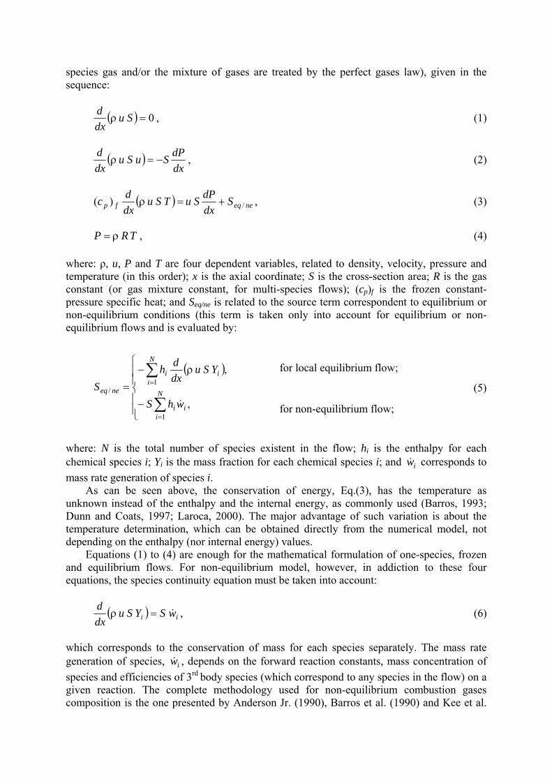
For frozen flow, the chemical composition is kept the same over all the flow. However, for local equilibrium flow, the composition must be recalculated at each control volume. Because of this, each chemical reaction scheme presents a different mass fraction profile. Figure 3 shows the H2O mass fraction profile for different chemical schemes implemented at Mach1D code. Again, the chemical reaction schemes that have better results (when compared

with CEA) are the six-species and eight-species models (represented in Fig. 3 by models 3 and 10, in this order).

Figure 3 - H2O mass fractions profiles along the nozzle, for

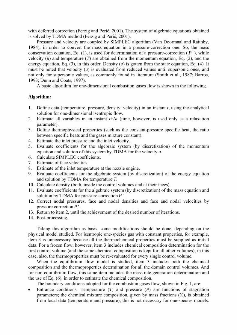
local equilibrium flow (80-volumes grid). Not only for H2O mass fraction profile, but also for other species are the results obtained from Mach1D close to those ones from CEA, as can be seen at Figs. 4 and 5. Nine chemical species were considered for simulations at CEA (the same eight from models 9 and 10 from Mach1D and also the ozone, O3); however, as the ozone mass fraction profiles were always below 5 x10-6, they were not shown in CEA results chart, and for this reason, it was not present in neither figures.

Figure 4 - Mass fractions profiles along the nozzle, for local equilibrium flow (Mach1D,

model 10, compared to CEA results) for H2O, O2, H2 and OH (80-volumes grid). 6.3 Parameters of interest Tables 4 and 5 supply numerical results for all the analyses made, including numerical error estimates by GCI estimator, for an 80-volumes grid. It can be seen that both six-species and eight-species models present the same numerical results and, also, both of them include

CEA ones, for frozen flow model. Similar results were obtained for local equilibrium flow; the six-species and eight-species Mach1D results, however, do not include CEA ones for all the variables (such as exit velocity and exit Mach’s number), although they are close to each other (the differences are below 3%). Based on this, both six and eight-species models seem to be the most adequate ones for studies involving frozen and/or local equilibrium flow.

Figure 5 - Mass fractions profiles along the nozzle, for local equilibrium flow (Mach1D,

model 10, compared to CEA results) for O, H, HO2 and H2O2 (80-volumes grid).

Table 4. Comparison for Cd, F* and Pex (80-volumes grid).

Model Cd [adim.] F* [adim.] Pex [Pa] 2.917342x104Analytical (R1) 1.0 1.0

Constant Properties (R1) 1.000 ± 3x10-3 1.001 ± 4x10-3 2.912x104 ± 8x101

Variable Properties (R1) 0.992 ± 3x10-3 1.004 ± 4x10-3 3.005x104 ± 4x101

Variable Properties (R2) 1.060 ± 3x10-3 1.004 ± 4x10-3 3.005x104 ± 4x101

Frozen Flow – mod. 0 1.060 ± 3x10-3 1.004 ± 4x10-3 3.005x104 ± 7x101



Frozen Flow – mod. 3, 4, 5 and 7 1.001 ± 3x10-3 1.000 ± 4x10-3 2.74x104 ± 1x102

Frozen Flow – mod. 9 and 10 1.001 ± 3x10-3 1.000 ± 4x10-3 2.74x104 ± 1x102

2.7448x104CEA (frozen flow) 1.000580 0.998992 Equilibrium Flow – mod. 0 1.060 ± 9x10-4 1.00 ± 1x10-2 3.005x104 ± 7x101

Equilibrium Flow – mod. 1 1.02 ± 1x10-2 1.01 ± 1x10-2 3.37x104 ± 3x102

Equilibrium Flow – mod. 2 1.00 ± 1x10-2 1.01 ± 1x10-2 3.54x104 ± 5x102

Equilibrium Flow – mod. 3, 4, 5 and 7 0.98 ± 1x10-2 1.01 ± 1x10-2 3.63x104 ± 5x102

Equilibrium Flow – mod. 9 and 10 0.98 ± 1x10-2 1.01 ± 1x10-2 3.63x104 ± 5x102

3.6178x104CEA (local equilibrium flow) 0.977372 1.011553 Non-equilibrium Flow – mod. 31 1.008 ± 3x10-3 1.012 ± 5x10-3 3.175x104 ± 7x101

Non-equilibrium Flow – mod 32 1.007 ± 3x10-3 1.014 ± 5x10-3 3.254x104 ± 6x101

Non-equilibrium Flow – mod. 5 1.007 ± 3x10-3 1.015 ± 5x10-3 3.359x104 ± 5x101



(R1): Rg = 526.97 J/kg ּK; (R2): Rg ≈ 461.53 J/kg ּK (equivalent to combustion gases mixture for the ideal model)

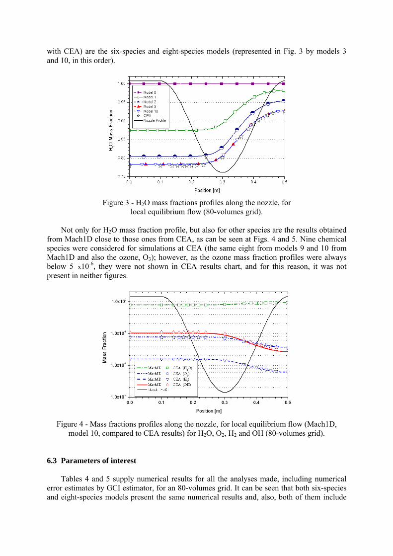
Tables 6 and 7 supply numerical results for all the analyses made, including numerical error estimates by GCI estimator, for a 2560-volumes grid. These tables, unfortunately, do not include results for non-equilibrium models 5, 7 and 10 (as well as equilibrium models 5, 7 and 9), by time restrictions. As expected, the grid refinement provides better numerical results (as can be seen by a comparison among Tables 4 to 7); exception is done for equilibrium temperature, for which the 80-volumes grid present results closer to CEA than ones obtained for the 2560-volumes grid. The differences between Mach1D and CEA results are, at maximum, of 0.28% for frozen flow and 2.51% (both for exit Mach’s number) for equilibrium flow, using an 80-volumes grid; when a 2560-volumes grid is used, these differences drop to 0.08% for frozen flow and 2.39% for equilibrium (also both for exit Mach’s number). This reduction, however, is quite small, when compared to the larger CPU time consumption demanded by the grid refinement.

Table 5. Comparison for Tex, uex and Mex (80-volumes grid).

Model Tex [K] uex [m/s] Mex [adim.] Analytical (R1) 1712.7409 3316.7150 3.1928346

Constant Properties (R1) 1710 ± 7 3319 ± 7 3.20 ± 1x10-2

Variable Properties (R1) 1800 ± 7 3357 ± 7 3.15 ± 1x10-2

Variable Properties (R2) 1800 ± 7 3142 ± 6 3.15 ± 1x10-2

Frozen Flow – mod. 0 1800 ± 7 3142 ± 6 3.15 ± 1x10-2

Frozen Flow – mod. 1 1713 ± 8 3221 ± 7 3.19 ± 1x10-2

Frozen Flow – mod. 2 1660 ± 8 3262 ± 7 3.21 ± 1x10-2

Frozen Flow – mod. 3, 4, 5 and 7 1606 ± 9 3312 ± 7 3.24 ± 1x10-2

Frozen Flow – mod. 9 1606 ± 9 3312 ± 7 3.24 ± 1x10-2

CEA (frozen flow) 1607.91 3311.4519 3.231 Equilibrium Flow – mod. 0 1800 ± 2x101 3142 ± 2x101 3.15 ± 3x10-3

Equilibrium Flow – mod. 1 2171 ± 4 3282 ± 3 2.998 ± 6x10-3

Equilibrium Flow – mod. 2 2345.9 ± 1x10-1 3354.3 ± 1x10-1 2.9357 ± 3x10-4

Equilibrium Flow – mod. 3, 4, 5 and 7 2461.2 ± 3x10-1 3427 ± 2 2.911 ± 2x10-3

Equilibrium Flow – mod. 9 and 10 2461.4 ± 3x10-1 3427 ± 2 2.911 ± 2x10-3

CEA (local equilibrium flow) 2462.41 3432.7056 2.986 Non-equilibrium Flow – mod. 31 1910 ± 1x101 3332 ± 6 3.05 ± 1x10-2

Non-equilibrium Flow – mod 32 1980 ± 1x101 3338 ± 6 3.02 ± 1x10-2

Non-equilibrium Flow – mod. 5 2059 ± 9 3344 ± 6 2.98 ± 1x10-2

Non-equilibrium Flow – mod. 7 2117 ± 8 3344 ± 6 2.96 ± 1x10-2

Non-equilibrium Flow – mod. 10 1910 ± 1x101 3332 ± 6 3.05 ± 1x10-2


Taking into account the numerical error estimates, both six-species and eight-species models present the same results (or at least, the values belong to the same numerical range) for frozen and local equilibrium flows. The unique exception is made for local equilibrium exit temperature, for which both chemical schemes present only one common value over their result ranges. Based on this, at least for the temperature and pressure ranges found in this work (pressure ranges up to 2.0 MPa and temperatures as high as 3400 K), the effect of using chemical reaction schemes with more than six species is nearly null, having influence only on computational efforts (and CPU time requirements). From Tables 4 to 7, it is seen that non-equilibrium results, as expected, are always between frozen and local equilibrium ones. When the behaviour of thermochemical properties is observed along the whole nozzle structure (Figs. 6 and 7), otherwise, a H2O mass fraction decrease is observed associated to a temperature drop at the beginning of the flow. Based on

results shown in Table 8, in which mass generation rates for H2O are presented, there are significant negative mass generation rates, especially for high values of pressure and temperature (condition found at the combustion chamber). Because of this negative mass rate generation, in order to keep atomic mass conservation, new species must be formed (such as O, H and OH). For these new species formation, however, endothermic reactions take place and, therefore, diminish the temperature of the whole gases mixture, as well as the H2O mass fraction at the beginning of the nozzle structure. It also can be seen that the numerical results of the five chemical schemes present the same numerical results (including the errors estimates) for both Cd and F*, for an 80-volumes grid. Because of this, for this grid, any of these chemical schemes can be used.

Table 6. Comparison for Cd, F* and Pex (2560-volumes grid).

Model Cd [adim.] F* [adim.] Pex [Pa] Analytical (R1) 1.0 1.0 29,173.42

Constant Properties (R1) 0.999999 ± 1x10-6 1.000000 ± 1x10-6 29,173.3 ± 2x10-1

Variable Properties (R1) 0.991754 ± 1x10-6 1.003224 ± 1x10-6 30,098.3 ± 2x10-1

Variable Properties (R2) 1.059739 ± 1x10-6 1.003224 ± 1x10-6 30,098.3 ± 2x10-1

Frozen Flow – mod. 0 1.059711 ± 1x10-6 1.003224 ± 1x10-6 30,098.6 ± 2x10-1



Frozen Flow – mod. 3, 4, 5 and 7 1.001086 ± 1x10-6 0.998998 ± 1x10-6 27,460.1 ± 2x10-1

Frozen Flow – mod. 9 and 10 1.001094 ± 1x10-6 0.998998 ± 1x10-6 27,460.7 ± 2x10-1

CEA (frozen flow) 1.000580 0.998992 27,448 Equilibrium Flow – mod. 0 1.059711 ± 3x10-6 1.003224 ± 4x10-6 30,098.6 ± 6x10-1

Equilibrium Flow – mod. 1 1.0190 ± 1x10-4 1.00884 ± 1x10-5 33,610 ± 1x101


Equilibrium Flow – mod. 3 and 4 0.9782 ± 1x10-4 1.011582 ± 8x10-6 36,160 ± 2x101


CEA (local equilibrium flow) 0.977372 1.011553 36,178 Non-equilibrium Flow – mod. 31 1.007717 ± 2x10-6 1.011741 ± 1x10-6 31,804.9 ± 4x10-1

Non-equilibrium Flow – mod 32 1.006824 ± 5x10-6 1.012647 ± 1x10-6 32,592.3 ± 7x10-1


Figure 6 - H2O mass fractions profiles along the nozzle, for

non-equilibrium flow (80-volumes grid).

Table 7. Comparison for Tex, uex and Mex (2560-volumes grid).

Model Tex [K] uex [m/s] Mex [adim.] Analytical (R1) 1712.7409 3316.7150 3.1928346

Constant Properties (R1) 1712.739 ± 7x10-3 3316.717 ± 7x10-3 3.19284 ± 1x10-5

Variable Properties (R1) 1802.338 ± 7x10-3 3355.079 ± 7x10-3 3.14424 ± 1x10-5

Variable Properties (R2) 1802.338 ± 7x10-3 3139.835 ± 7x10-3 3.14424 ± 1x10-5

Frozen Flow – mod. 0 1802.450 ± 7x10-3 3139.920 ± 7x10-3 3.14424 ± 1x10-5



Frozen Flow – mod. 3, 4, 5 and 7 1609.141 ± 9x10-3 3309.743 ± 7x10-3 3.23078 ± 1x10-5


CEA (frozen flow) 1607.91 3311.4519 3.231 Equilibrium Flow – mod. 0 1802.45 ± 2x10-2 3139.92 ± 2x10-2 3.14424 ± 4x10-5



Equilibrium Flow – mod. 3 and 4 2459.8 ± 2x10-1 3429.8 ± 5x10-1 2.9147 ± 6x10-4


CEA (local equilibrium flow) 2462.41 3432.7056 2.986 Non-equilibrium Flow – mod. 31 1915.20 ± 4x10-2 3329.958 ± 3x10-3 3.04829 ± 2x10-5

Non-equilibrium Flow – mod 32 1980.9 ± 1x10-1 3335.89 ± 1x10-2 3.01833 ± 4x10-5


Table 8. Mass generation rates [kg/m3.s] for H2O (based on equilibrium composition).

Conditions Model 31 Model 32 Model 5 Model 7 Model 10 T = 4,000 K; P = 20 MPa -1.538x109 -1.263x109 -1.538x109 -1.263x109 -1.537x109

T = 3,000 K; P = 20 MPa -3.914x107 -4.965x107 -3.914x107 -4.965x107 -3.914x107

T = 3,000 K; P = 2 MPa -3.612x105 -4.407x105 -3.612x105 -4.407x105 -3.612x105

T = 2,000 K; P = 200 kPa -6.687x10-1 -1.310x100 -6.687x10-1 -1.310x100 -6.687x10-1

T = 1,500 K; P = 20 kPa -7.136x10-7 -1.873x10-6 -7.136x10-7 1.873x10-6 -7.136x10-7

Figure 7 – Temperature profile along the nozzle, for non-equilibrium flow (80-volumes grid).

6.4 Grid considerations A last observation is about the grids used in this work: most of tables and figures show results for an 80-control-volumes-grid. Even though more refined grids were employed (at maximum, with 10240 control volumes), the 80-control-volumes-grid results were preferred; this is because the estimated numerical errors are about the same magnitude of experimental errors (Marchi et al., 2004). Besides, the CPU time requirement for an 80-control-volumes-grid is much lower than for a 10240-control-volumes-grid (or even a 2560 one). The CPU time consumption for an 80-volumes grid is at least 40 times lower than for a 2560-volumes grid for isentropic, one-species flow with constant properties (3.1 s against 2.1 min); for equilibrium flow, however, the difference is even greater: it achieves more than 1200 times (2.3 min against 2 days). For non-equilibrium flow, otherwise, the differences in CPU time are reduced to about only 6 times (17 min against 1.7 h, for model 31; and 27 min against 2.6 h, for model 32). This reduction in CPU time differences is explained by the reduction in the number of iterations needed for convergence: it was observed that, until the 160-volumes-grid, for numerical convergence, the number of iterations increase with the grid refinement (as occurred for other physical models); for more refined grids, however, this number of iterations has begun to decrease with grid refinement. Because of this, while for the 80-volumes-grid 5.0x106 iterations were needed (for model 31), for the 2560-volumes-grid, only 1.0x106 iterations were enough for convergence. Similar behaviour was seen for model 32, in which, for the 80-volumes-grid 1.5x107 iterations were used and, for the 2560-volumes-grid, only 1.5x106 iterations were necessary. 7. CONCLUSION Differently as usually found in literature, the energy equation has the temperature as unknown (instead of the enthalpy and the internal energy). The major advantage of such variation is about the temperature determination, which is done directly from the numerical model. Also, the velocity determination is done from the combustion chamber to the nozzle exit, covering all the velocity regimes in a real engine (subsonic, transonic and supersonic ones), and not only the supersonic flow, as commonly done. Six and eight-species models have shown the same numerical results for nearly all thermoproperties. Because of this, at least for the temperature and pressure conditions found in this work (up to 3400 K and 2.0 MPa), the effect of using chemical reaction schemes with more than six species is nearly null, having influence only on computational efforts (and CPU time requirements). The choice of a chemical scheme is also very important for CPU time, for local equilibrium flow: comparing the four 6-species schemes, for an 80-volumes-grid, it was observed that simulations with models 3 and 4 took less than 3 minutes, while the same simulations with models 5 and 7 lasted more than 4 hours – at least 120 times more. The same behaviour was observed for the eight-species models. Furthermore, reaction schemes with larger number of reaction equations present a lower quantity of significant figures, possibly by numerical errors associated to the greater numerical efforts for the solution achievement. Based on these facts, it is recommended the use of models 3 and 4 (six-species schemes), at least for preliminary tests involving frozen and local equilibrium flows. Non-equilibrium results, for exit parameters, were always between frozen and local equilibrium ones. However, when the thermochemical profiles along the nozzle structure were studied, a decrease on H2O mass fraction associated to a temperature drop was verified.

A possible explanation for this phenomenon is based on the high negative mass generation rates at high pressure and high temperature (conditions found at the beginning of the flow), which allows the appearance of new chemical species (like H, O and OH), by endothermic chemical reactions, what reduces the gases mixture temperature. Most of the results were shown for an 80-control-volumes grid, because for this grid the magnitude of estimated numerical errors is equal to experimental ones. Otherwise, the CPU time consumption for an 80-volumes grid is at least 40 times lower than for a 2560-volumes grid (for isentropic, one-species flow with constant properties); for equilibrium flow, however, the difference is even greater: it achieves more than 1200 times (for model 3). It is the reasons for choosing an 80-volumes grid, at least for preliminary tests. Acknowledgements The authors would acknowledge Federal University of Paraná (UFPR), Coordenação de Aperfeiçoamento de Pessoal de Nível Superior (CAPES) and The “UNIESPAÇO Program” of The Brazilian Space Agency (AEB) by physical and financial support given for this work. The first author would, also, acknowledge his professors and friends, by discussions and other forms of support. The second author is scholarship of CNPq (Conselho Nacional de Desenvolvimento Científico e Tecnológico) – Brazil. REFERENCES Anderson Jr., J. D., 1990. Modern Compressive Flow. 2 ed., New York: McGraw-Hill. Barros, J. E. M., 1993. Escoamento Reativo em Desequilíbrio Químico em Bocais

Convergente-Divergente. M. Sc. Thesis. Technological Aeronautic Institute, São José dos Campos, Brazil.

Barros, J. E. M.; Alvin Filho, G. F.; Paglione, P., 1990. Estudo de escoamento reativo em desequilíbrio químico através de bocais convergente-divergente. In: III Encontro Nacional de Ciências Térmicas. Itapema: Anais...

Dunn, S. S., Coats, D. E., 1997. Nozzle Performance Predictions Using the TDK 97 Code. In: 33rd Joint Propulsion Conference and Exhibit, Seattle: Proceedings... AIAA 97–2807.

Ferziger, J. H., Perić, M., 2001. Computational Methods for Fluid Dynamics. 3 ed. Berlin: Springer-Verlag.

Fröhlich, A., Popp, M., Schmidt, G., Thelemann, D., 1993. Heat transfer characteristics of H2/O2 combustion chambers. In: 29th Joint Propulsion Conference. Monterrey: Proceedings… AIAA 93 – 1826.

Glenn Research Center, 2005. CEA – Chemical Equilibrium with Applications. Available in: <http://www.grc.nasa.gov/WWW/CEA Web/ceaHome.htm>. Access in: Feb 16, 2005.

Kee, R. J., GrCar, J. F., Smooke, M. D., Miller, J. A., 1990. A Fortran Program for Modeling Steady Laminar One-Dimensional Premixed Flames. Albuquerque: Sandia National Laboratories. SAND85-8240 · UC-401.

Kee, R. J., Rupley, F. M., Meeks, E., Miller, J. A., 1996. Chemkin-III: A Fortran Chemical Kinetics Package for the Analysis of Gas-Phase Chemical and Plasma Kinetics. Albuquerque: Sandia National Laboratories, SAND96-8216 UC-405, 1996.

Kuo, K. K., 1986. Principles of Combustion. New York: John Wiley & Sons. Laroca, F., 2000. Solução de escoamentos reativos em bocais de expansão usando o método

dos volumes finitos. M. Eng. Thesis. Federal University of Santa Catarina, Florianópolis, Brazil.

http://www.grc.nasa.gov/WWW/CEA%20Web/ceaHome.htm

Marchi, C. H., Araki, L. K., Laroca, F., 2005. Evaluation of thermochemical properties and

combustion temperatures for LOX/LH2 reaction schemes. In: 26th Iberian Latin-American Congress on Computational Methods in Engineering. Guarapari: Proceedings…

Marchi, C. H., Laroca, F., Silva, A. F. C., Hinckel, J. N., 2000. Solução numérica de escoamentos em motor-foguete com refrigeração regenerativa. In: 21st Iberian Latin American Congress on Computational Methods in Engineering. Rio de Janeiro: Proceedings…

Marchi, C. H., Laroca, F., Silva, A. F. C., Hinckel, J. N., 2004. Numerical solutions of flows in rocket engines with regenerative cooling. Numerical Heat Transfer, Part A, v. 45, pp. 699 – 717.

Marchi, C. H., Maliska, C. R., 1994. A nonorthogonal finite volume method for the solution of all speed flows using co-located variables. Numerical Heat Transfer, Part B, v. 26, pp. 293 – 311.

Marchi, C. H., Silva, A. F. C., 2002. Unidimensional numerical solution error estimation for convergent apparent order. Numerical Heat Transfer, Part B, v. 42. pp. 167–188.

Roache, P. J., 1994. Perspective: A method for uniform reporting of grid refinement studies. Journal of Fluids Engineering, v. 116, pp. 405-413.

Roache, P. J., 1998, Verification and Validation in Computational Science and Engineering, Hermosa Publishers.

Smith, T. A., Pavli, A. J.; Kacynski, K. J., 1987. Comparison of theoretical and experimental thrust performance of a 1030:1 area ratio rocket nozzle at a chamber pressure of 2413 kN/m2(350 psia). Cleveland: NASA Lewis Research Center. NASA Technical Paper 2725.

Sutton, G. P., Biblarz, O. 2001. Rocket Propulsion Elements. 7 ed. New York: John Wiley & Sons.

Svehla, R. A., 1964. Thermodynamic and transport properties for the hydrogen-oxygen system. Cleveland: NASA Lewis Research Center. NASA SP-3011.

Tannehill, J. C., Anderson, D., Pletcher, R. H., 1997. Computational Fluid Mechanics and Heat Transfer. 2 ed. Philadelphia: Taylor & Francis.

Van Doormaal, J. P., Raithby, G. D., 1984. Enhancements of the SIMPLE method for predicting incompressible fluid flow. Numerical Heat Transfer, v. 7, pp. 147 – 163.

xxix cilamce november 4 to 7 , 2008 maceió -...

Documents