Faster MIP Solutions via New Node SelectionRulesDaniel T. Wojtaszek John W. Chinneckdtwojtas@sce.carleton.ca chinneck@sce.carleton.caSystems and Computer EngineeringCarleton UniversityOttawa, Ontario K1S 5B6CanadaNovember 12, 2009AbstractWhen a branch and bound method is used to solve a linear mixed integer program(MIP), the order in which the nodes of the branch and bound tree are explored signi�-cantly a�ects how quickly the MIP is solved. In this paper, new methods are presentedthat exploit correlation and distribution characteristics of branch and bound trees totrigger backtracking and to choose the next node to solve when backtracking. A newmethod is also presented that determines when the cost of using a node selection methodoutweighs its bene�t, in which case it is abandoned in favor of a simpler method. Em-pirical experiments show that these proposed methods outperform the current state ofthe art.1 IntroductionLinear Mixed Integer Programs (MIP) can be formulated as follows.The objective function is de�ned as:minimize z =

∑

j∈I

ojxj +∑

j∈C

ojxjThe constraints are de�ned as:∑

j∈I

aijxj +∑

j∈C

aijxj {≤, =,≥} vi, i = 1, . . . , m

lj ≤ xj ≤ uj j ∈ I ∪ Cxj ∈ Z j ∈ Ixj ∈ R j ∈ C

I is the set of variables constrained to be integer valued (including binary-valued).C is the set of continuous, real valued variables.1

Many methods for solving MIPs employ a branch and bound solution method. The generalprocedure of branch and bound is summarized in Algorithm 1. A di�culty with branch andbound is that it can take an impractical amount of time to solve some MIPs, even when usingthe most sophisticated computers. For this reason, the focus of this work is on developingfaster methods for solving MIPs.The performance of the branch and bound method is greatly a�ected by the choice ofthe branching variable selection method (Step 4), and the node selection method (Step 2).After solving the LP relaxation of the current node (Step 3), there will be a list of candidatevariables, i.e. variables that are required to take integer values and yet are not integer-valuedin the current LP-relaxation optimal solution. The branching variable selection methodchooses a candidate variable from the list for branching. This produces two child nodes: inone child node the lower bound of xj is set to the nearest integer value that is greater thanthe LP-relaxation solution value of xj , and in the other child node the upper bound is set tothe nearest integer that is less than the value of xj .In Step 2, if there are two or more unexplored (active) nodes then the node selectionmethod determines which active node to solve next. As far as possible, the goal is to choosenodes that are ancestors of a MIP optimal node so that the resulting tree is as small aspossible, though there is no guaranteed method for making an accurate selection. Thereare numerous node selection heuristics that try to achieve this goal, or that use some otherstrategy of developing the branch and bound tree to achieve a di�erent goal, such as reachinga �rst feasible solution quickly. The node selection heuristic can have a dramatic e�ect onthe solution e�ort. For example, for the bell4 model from MIPLIB 2.0, GLPK does notsolve this model within 1 hour using its default node selection method, whereas this modelis solved in 10.66 seconds when using one of the new node selection methods developed here.This paper develops new heuristics for node selection that demonstrate signi�cant im-provement over state of the art methods in solving MIPs to optimality quickly. There arethree aspects to the new methods: (i) determining when to backtrack, i.e. to select a nodeother than a child of the node most recently explored, (ii) determining which node to back-track to, and (iii) determining when to abandon an advanced but costly backtrack selectionmethod in favour of simple depth-�rst search.1.1 Existing Node Selection HeuristicsSince the LP-relaxation solution is not yet available, the lower bound of an unexplored nodeis initially set equal to that of its parent node. The same is true for any other LP solutioncharacteristics of a node such as the number of candidate variables. Using the availableinformation, node selection heuristics try to avoid choosing super�uous nodes, i.e. nodeswhose lower bound turns out to be greater than the (unknown) MIP optimal objectivevalue, z∗.The best-�rst, or best-bound, node selection method avoids the exploration of super�uousnodes by choosing the unexplored node having the smallest lower bound over all the unex-plored nodes. Nodes that are closer to the root node are more likely to be chosen becausetheir lower bounds are generally smaller than the lower bounds of nodes deeper in the tree.Since MIP feasible solutions usually occur at leaf nodes that are far from the root node,best-�rst search is not a good choice for quickly �nding a MIP feasible solution. This is2

Algorithm 1 Branch and BoundInputs: MIP instance.Initialize: Incumbent solution, I = φ. Objective value of incumbent solution, z(I) = ∞.List of unexplored nodes, N = φ.Procedure:1. Add the initial LP-relaxation (the root node) to N .2. Choose a node from N for exploration and label it currentNode.3. Solve the LP-relaxation for currentNode.• If LP-relaxation is infeasible or it is feasible with a lower bound that is greaterthan z(I) then discard currentNode and go to Step 7.• If LP-relaxation is MIP feasible then:� If LP-relaxation objective function value is less than z(I) then replace I withthis solution, else discard currentNode.� Go to Step 74. Choose a candidate variable in currentNode for branching.5. Branch on the selected variable to create two child nodes of currentNode; add thesenodes to N . Remove currentNode from N .6. Go to Step 27. If list of unexplored nodes is empty then:7.1 If I = φ, then exit with infeasible outcome.7.2 Optimum is I: exit with optimal outcome.8. Go to Step 2

3

also true of the breadth-�rst node selection method, which chooses the earliest created activenode.Depth-�rst node selection always chooses a child of the most recently explored node.Given the two child nodes created by branching on a variable, a heuristic is used to choosewhich one to explore next. Some common methods for making this branch direction decisioninclude choosing the up branch, the down branch, the branch that has the nearest integerbound for the branching variable, or the branch that forces the value of the branching variableaway from its value at the root node [22]. If the last solved node is either LP infeasible, MIPfeasible, or worse than the incumbent solution, then the last created active node is explored.Depth-�rst node selection is a better choice if the goal is to �nd a MIP feasible solution asquickly as possible.A major advantage of depth-�rst exploration of the tree is that the LP formulations for aparent and a child node di�er by only a single variable bound, which means that the solutionof the child node can be hot-started, and hence is very quick. Other node selection methodsthat do not move from parent to child node in succession cause the solution of dissimilarLPs in succession, and hence the average number of simplex iterations to solve each nodeis usually signi�cantly higher as compared to depth-�rst node selection [5, 11, 20]. Thisassumes that the factorized simplex basis of only the most recently solved node is availablewhich, due to computer memory limitations, is true for most MIP solvers. Depth-�rst searchalso tends to maintain fewer unexplored nodes in memory, and hence is less likely to exhaustthe available memory. Some MIP solvers, such as SCIP [3], use a prede�ned threshold ofmemory usage to ensure that the size of the branch and bound tree does not exceed theavailable memory by switching to depth-�rst node selection if this threshold is exceeded.A number of node selection schemes try to combine the advantages of the best-�rst anddepth-�rst methods. One such scheme uses depth-�rst search until a MIP feasible solutionis found and then switches back and forth between best-�rst and depth-�rst strategies [5].The most-feasible node selection method chooses the node with the smallest sum of frac-tional values over all candidate variables. This is useful in seeking integer-feasible solutions.Knowing the value of z of the best possible MIP feasible solution attainable at a descen-dent of a given node would be useful in selecting which node to explore. Methods whichestimate this value, called estimate based methods, include the best-projection method [16, 23]and the best-estimate method [6, 14].The best-projection method uses the change in the value of z between the root node andthe incumbent solution as well as the change in the sum of integer infeasibilities betweenthe root node and the node for which the estimate is being computed. The best projectionestimate at node i is computed as follows:Ei = zi +

(

zinc − z0

s0

)

siwhere zi is the lower bound of node i, zinc is the value of z for the incumbent solution, z0is the lower bound of the root node, s0 is the sum of integer infeasibilities at the root node,and si is the sum of integer infeasibilities at node i.The best-estimate method uses pseudo-costs. Each integer variable has two pseudo-costvalues associated with it, one for the up branch, P Uj , and the other for the down branch,

P Dj . When a variable is branched on, the change in the lower bound between the parent4

node and the down child node is ∆zDj = zD

j − zPj where zD

j is the lower bound for the downchild node and zPj is the lower bound for the parent node. Likewise for the up child node

∆zUj = zU

j − zPj . The pseudo-cost value for the down branch of xj is

P Dj = ∆zD

j /fjand similarly for the up branchP U

j = ∆zUj /(1 − fj)where fj is the fractional value of xj . Note that fj is greater than 0 since only variablesthat are not integer feasible can be branched on. Updating the pseudo-costs for xj is typicallydone by averaging the values from every instance that xj was branched on. The estimate ofthe best integer feasible solution attainable from a node i is calculated as follows:

Ei = zi +∑

j∈I

min{P Dj fj , P

Uj (1 − fj)}.In these methods the active node with the smallest such estimate is explored next.Linderoth and Savelsbergh [20] considered the pseudo-cost estimates to be optimistic, sothey proposed an adjusted pseudo-cost estimate. Achterberg [2] proposed interleaving best-estimate with best-�rst node selection by performing best-�rst node selection once for every

bfq best-estimate backtracking node selections. It is suggested that bfq = 9 should be used.Forrest et al [14] proposed a method that uses best-estimate node selection until a MIPfeasible solution is found and then chooses nodes according to the percentage error criterion.Backtracking node selection uses depth-�rst search until the current node is either MIPfeasible, LP infeasible, has a lower bound that is greater than the value of z of the incumbentsolution, or is considered undesirable to explore, at which point backtracking occurs. Abacktracking node selection method is then used to select the next node to explore insteadof choosing a child of the current node, typically either the best-�rst, best-projection, orbest-estimate criterion [20]. Many implementations of the branch and bound method use anestimate z̃∗ of the MIP optimal objective value, called an aspiration value, in an attempt toavoid the exploration of super�uous nodes by triggering backtracking node selection whenthe lower bound of a node exceeds z̃∗. The aspiration value is typically set by the user beforethe branch and bound process begins. Various methods have been proposed to computez̃∗ including best-projection estimates [20] as well as some estimation methods based onpseudo-costs [15, 20].Kostikas and Fragakis [17] have experimented with using genetic programming to createcustomized node selection rules for a given MIP instance during the branch and boundsolution process of this instance.1.2 Room for ImprovementWe performed a proof-of-concept experiment to test the potential merit of using a goodaspiration value in a branch and bound procedure. We solved a set of MIP instances andrecorded the MIP optimum values. We then re-solved the instances using an aspirationvalue equal to the MIP optimal objective value. This reduced the total time to solve all of5

the test instances by 15% relative to the best existing aspiration method. It also reducedthe mean ratio to the best time to solve each MIP instance by 48% relative to the bestexisting aspiration method. This suggests that it is worthwhile to �nd ways of generatinggood estimates of the MIP optimal objective value for use in triggering backtracking.2 Backtrack Triggering and Node Selection HeuristicsBased on Frequent Patterns in MIP SolutionsThe new methods developed in this paper are:• the modi�ed best-projection backtracking node selection and aspiration methods;• the distribution backtracking node selection method;• the feasibility depth extrapolation aspiration method;• and the active node search threshold.2.1 Modi�ed Best Projection Node Selection and Aspiration MethodOur modi�cation to the best-projection method estimates the objective value of the bestMIP feasible solution attainable from any node using nodes that are not MIP feasible. Thiseliminates the need to �nd an incumbent solution before computing an estimate, as in theoriginal best projection method. The modi�ed version is used both to select a node duringbacktracking and to trigger backtracking. The modi�cation is based on Observation 1.A few de�nitions are needed. Let ci be the number of candidate variables at node i. Let

c0 be the number of candidate variables at the root node. Let zi be the objective value atnode i. Let z0 be the objective value at the root node. Let zmin(c) be the smallest zi overall nodes with c candidate variables:zmin(c) = min

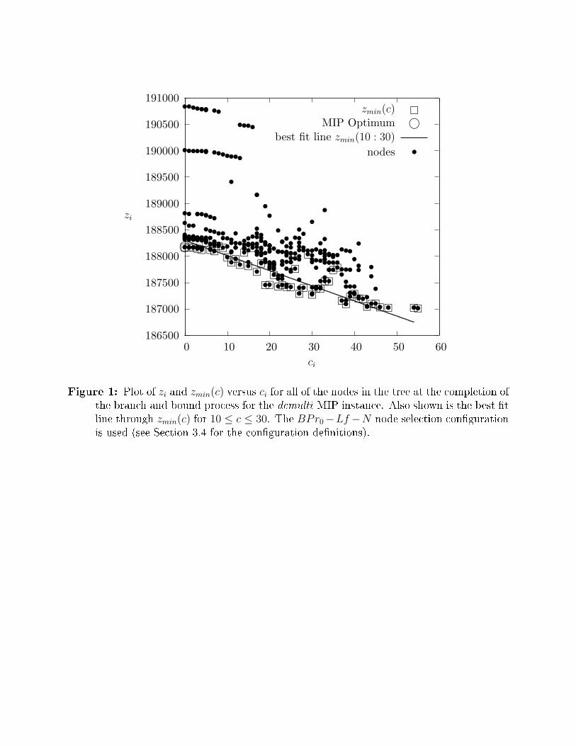
i{zi : ci = c}.Observation 1 (Node Infeasibility versus Optimality)There is an approximately linear correlation between zmin(c) and c for many MIPs. �For many MIP instances, plots of zmin(c) versus c show a trend that indicates the possi-bility of estimating the value of z∗ early in the branch and bound process by simple linearextrapolation. Note that z∗ occurs at zmin(0). For the dcmulti MIP instance, the trend canbe seen in Figure 1 for 10 ≤ c ≤ 30.Observation 1 underlies our improvement to the best-projection method. Recall thatin the best-projection method an incumbent solution is required to compute an estimateof the degradation in objective value per unit MIP infeasibility. At any time during thebranch and bound process, the incumbent solution objective value is zmin(0) which is theminimum objective value found at a node with 0 candidate variables, i.e. a MIP feasible node.According to Observation 1, a useful estimate of the degradation in objective value per unit6

186500

187000

187500

188000

188500

189000

189500

190000

190500

191000

0 10 20 30 40 50 60

zi

ci

zmin(c) �MIP Optimum ©

best fit line zmin(10 : 30)

nodes •

��������������

��

�

��

�������

�

��

�

�����

��

������

����� ��

©

••••••••••••

•••••••••

••

•

•

••••••••••

••••

•

••

••••••••••••••

••

••

•••••••••••

••• •

••••••

••• ••

••• ••• •

••• ••••••••

•••• •••

••••••••••••• •

••••••

• •••••••••• •

••

••••

•

••••••••

•••

••••••••••••

••••••

•••••

•• ••

••••••

•••

••••••

•

••••••

•••••••••••• ••

• ••••••

•••

••

••

••

•••••

•••••

••

•••••

••••••••

•••••••• ••••• ••• • ••••••• • •••

••••••••• ••••

••••

•••• ••••••••• ••••• •••••

••• •

•••••

••••••••••••

•• •••••••••

Figure 1: Plot of zi and zmin(c) versus ci for all of the nodes in the tree at the completion ofthe branch and bound process for the dcmulti MIP instance. Also shown is the best �tline through zmin(c) for 10 ≤ c ≤ 30. The BPr0−Lf −N node selection con�gurationis used (see Section 3.4 for the con�guration de�nitions).

MIP infeasibility can be made using zmin(c) for c > 0 thus allowing modi�ed best-projectionnode selection to proceed without an incumbent solution.The following de�nitions are needed for this algorithm. Let cmin be the minimum numberof candidate variables over all nodes solved so far. This value is initially equal to the numberof candidate variables at the root node and is updated after each node is solved. Let σz bethe standard deviation of zi over all nodes solved so far. Let σc be the standard deviationof ci over all nodes solved so far.The estimate of degradation of the objective value per unit change in MIP infeasibility,m, is computed as follows:

m =zmin(cmin) − z0

c0 − cmin

. (1)The estimate of the objective value of the best MIP feasible solution attainable from anode i, z̃∗i , is computed as follows:z̃∗i = ci ∗ m + zi.The value of −m is the slope of the line through (cmin, zmin(cmin)) and (c0, z0). Figure 2shows an example of this line at a time in the branch and bound process when cmin = 23,

c0 = 55 (the number of candidate variables at the root node), zmin(cmin) = 187, 851.53,and z0 = 187, 022.36 (the objective value at the root node). The slope of the line throughthe points (cmin, zmin(cmin)) and (c0, z0) is −m = −25.91. At this time the value of zi =zmin(cmin) for the most recently solved node i. Likewise, the value of ci = cmin. An estimate ofthe objective value of the best MIP feasible solution attainable from node i, is z̃∗i = 188, 447.5.This estimate is the extrapolated value of zmin(0) using the line through (ci, zi) with a slopeequal to −m.If at least one of the following conditions is satis�ed then this method does not work well.

• cmin = c0. In this case the denominator in (1) is 0.• σc < σmin

c , where σminc is the minimum acceptable value of σc. In this case most nodeshave very similar values of ci. This causes the value of m to have little e�ect on nodeselection. We set σminc = 3.

• σz < σminz , where σmin

z is the minimum acceptable value of σz. In this case there isvery little change in zi over all nodes. This causes the value of m to be almost 0 whichthen results in ci having little e�ect on node selection. We set σminz = 0.001.The thresholds used for the last two conditions were determined empirically. None of theMIP instances where modi�ed best-projection worked well satis�ed any of these conditions.In most cases where it did not work well, at least one of these conditions was satisi�ed.2.2 Distribution Node SelectionThis backtracking node selection method balances the goals of MIP feasibility and MIP op-timality. It uses probability distributions of measures of MIP feasibility and MIP optimalitythat are based on data taken from all nodes solved so far in the solution process. This7

187000187200187400187600187800188000188200188400188600

0 10 20 30 40 50 60

zi

ci

dcmulti

nodes

••••••••••

••

•

•line through zmin(55) and zmin(23)

MIP optimum© ©zmin(c)

������

����

��

Figure 2: Plot of zi and zmin(c) versus ci for all of the nodes in the tree at the time in thebranch and bound process when cmin = 23 for the dcmulti MIP instance. Most of thepoints in the plot overlap because zi = zmin(c) for most of the nodes at this time. Alsoshown is the line through zmin(55) (the root node) and zmin(23).

approach weights the MIP feasibility and optimality goals dynamically so that neither candominate the other for too long. It favours choosing nodes with lower objective values andless MIP infeasibility.The most commonly used measure of a node's closeness to optimality is its value of z.The measure of MIP infeasibility used in this method is the number of candidate variables c.The number of candidate variables is used instead of the sum of the fractional componentsof the integer variables because a candidate variable will likely become integer valued if thatvariable is branched on regardless of what its fractional value is. For example, suppose onenode has one candidate variable with a fractional value of 0.5 whereas another node has �vecandidate variables each with a fractional value of 0.09. If all other integer variables are �xedfor both of these nodes, then choosing the �rst node will likely lead to a MIP feasible nodemore quickly than choosing the second node, which has a lower sum of integer infeasibilities.Observation 2 (Balancing MIP Feasibility and Optimality)A characteristic that is typical of many branch and bound trees is that there is a negativecorrelation between the objective value and the number of candidate variables of a node; i.e.zi tends to increase with depth while ci tends to decrease with depth. �A consequence of Observation 2 is that when trying to balance MIP feasibility and MIPoptimality during node selection, if greater weight is being given to zi than to ci, then thefraction of nodes chosen with small zi will likely be large relative to the fraction of nodeschosen with small ci. The opposite is likely true if greater weight is given to ci than to zi.Note that MIP feasibility is reached when ci = 0.Since it is desirable to choose nodes with both small zi and small ci, these values needto be combined into a single value in order to rank all of the active nodes. This combinedvalue should be directly proportional to both zi and ci. Combining zi and ci so that neitherdominates the other can be di�cult due to the di�erence between the range of zi and therange of ci across all of the nodes. For example, Figure 1 shows that the range of zi fordcmulti is over 3000, whereas the range of ci is less than 60. This problem is solved byassembling the probability distributions of zi and ci, respectively, as data becomes availableduring the solution process. Note that the range of each distribution is [0, 1] and that eachdistribution is a monotonically increasing function of its independent variable.The distribution function used in this method is suggested by the Central Limit Theorem,which states that, under certain conditions, the distribution of a sum of random variablestends to a Normal distribution. Although the underlying process that determines the valueof each variable at a node is not random, it is not usually easy to predict the value of everyvariable at a node before it is solved. Therefore the variables can be thought of as randomvariables whose values are measured each time an active node is solved. The value of zifor a node is a weighted sum of these variables, therefore a Normal distribution is used toestimate the distribution of zi in a branch and bound tree. The value of ci can be thoughtof as the sum of a set of random variables where each integer variable adds either 0 or 1 toci depending on whether it is integer or fractional valued respectively. Therefore, a Normaldistribution is used to estimate the distribution of ci. In addition, the Normal distributionis well suited for balancing the pursuit of MIP feasibility with optimality since (i) it requireslittle more work to compute than the Uniform distribution, (ii) it estimates the values of zi8

and ci that most frequently appear in the tree using their respective means mz and mc, and(iii) it uses information on the ranges of zi and ci via their respective standard deviations σzand σc.Let FZ(z) = P (Z ≤ z) and FC(c) = P (C ≤ c) be estimates of the Normal cumulative dis-tribution functions for zi and ci, respectively, over all nodes solved so far. The value of FZ(zi)is the estimated fraction of nodes with a value of z ≤ zi. Similarly, the value of FC(ci) is theestimated fraction of nodes with a value of c ≤ ci. The distribution backtracking node selec-tion method chooses an active node with the smallest value of FZC(zi, ci) = FZ(zi) × FC(ci)to be explored next. This FZC(zi, ci) is used as the comparison criterion because its value isdirectly proportional to both FZ(zi) and FC(ci), and FZC(zi, ci) ≤ min(FZ(zi), FC(ci)) (recallthat 0 ≤ FZ(zi) ≤ 1, and 0 ≤ FC(ci) ≤ 1) which causes this node selection method to behavea little like a combination of the best-�rst and the most-feasible node selection methods.The following example demonstrates how the pursuit of MIP feasibility and optimalitycan be balanced using Normal distributions. Suppose that during backtracking node selectionthere are 4 LP feasible nodes in the tree, two of which have 1 unsolved child each. The valuesof zi and ci for each LP feasible node are given below.i zi ci child0 1 100 n11 100 12 100 13 100 1 n2In this example, one of the candidate nodes is the unsolved child n1 of node 0, and theother is the unsolved child n2 of node 3. Recall that the value of zi and ci at an unsolvednode is initially set to its parent's value of zi and ci respectively. The choice of which node tosolve next is between node n1 which has a small value of zi and a large value of ci, and node

n2 which has a large value of zi and a small value of ci. To emphasize the optimality goal,we would like to choose the node i that has the smallest fraction of nodes with z ≤ zi, but toemphasize the feasibility goal, we would like to choose the node i having the smallest fractionof nodes with c ≤ ci. Estimates of these fractions are computed for our example using FZ(zi)and FC(ci), and are given below along with the product of these fractions FZC(zi, ci) for eachcandidate node.i FZ(zi) FC(ci) FZC(zi, ci)

n1 0.067 0.933 0.062n2 0.691 0.309 0.213Node n1 has the smallest value of FZC(zi, ci) so it is chosen to be solved next. Node n1 islikely the better choice because three of the nodes have a large value of zi and a small valueof ci whereas one of the nodes has a small value of zi and a large value of ci. This indicatesthat more emphasis has been placed on the pursuit of MIP feasibility than the pursuit ofoptimality so the emphasis should be shifted towards the pursuit of optimality by selectingnode n1 to be solved next.The distribution backtracking node selection method computes FZC(zi, ci) for each activenode i. The node n that will be explored next is chosen as follows:9

n = arg mini

FZC(zi, ci).If there is very little variation in the value of zi, or if ci does not change signi�cantly inproportion to the depth of the nodes in the tree, then this method does not work well sinceone of the measures will be given too much weight in node selection. This is summarized inthe following two conditions. Let d be the depth of the latest solved node before backtrackingnode selection.• σc/d < σmin

cd : In this case most nodes have very similar values of ci over a large rangeof depths in the tree. We set σmincd = 0.1.

• σz < σminz : In this case there is very little change in zi over all nodes. We set σmin

z =0.001.The thresholds used for these conditions were determined empirically. No instances wheredistribution node selection worked well satis�ed either condition. Most instances wheredistribution node selection did not work well satis�ed at least one of these conditions.2.3 Feasibility Depth Extrapolation AspirationThis method estimates the MIP optimal objective value by �rst estimating the depth of theMIP optimal node via linear extrapolation of the number of candidate variables along theancestors of each node in the branch and bound tree. The MIP optimal objective functionvalue is then estimated based on the node optimum values at that depth. This method isbased on Observations 3, 4 and 5.Observation 3 (MIP Optimal Depth and Objective Value)The largest objective value over all nodes at the depth of a MIP optimal node in thebranch and bound tree is greater than or equal to the MIP optimal objective value. �Observation 4 (Relative Depth of MIP Optimal Node)The MIP optimal node in the branch and bound tree tends to be closer to the root nodethan most other MIP feasible nodes (i.e. less deep than other MIP feasible nodes). �Observation 5 (Node Infeasibility versus Depth) Extrapolating the rate of decreaseof the number of candidate variables along a dive in the branch and bound tree provides areasonable estimate of the depth of the �rst MIP feasible solution for the dive. �Figure 3 demonstrates Observation 3 for the bell5 instance. As shown, the largest ob-jective value over all nodes at the MIP optimal depth is less than the objective values of asigni�cant number of nodes in the tree. Therefore, if the largest objective value over all nodesat the MIP optimal depth is known and is used as an aspiration value, then the amount ofe�ort required to solve this MIP instance will be reduced, without danger of eliminating theoptimal solution. Figure 3 also shows that nodes that are close to a MIP optimal depth tendto have objective values that are relatively close to the MIP optimal objective value. Thissuggests a method of estimating a suitable aspiration value. Finally, Figure 3 shows that10

8.6e+068.8e+06

9e+069.2e+069.4e+069.6e+069.8e+06

1e+071.02e+07

0 200 400 600 800 1000 1200

zi

di

bell5

z∗

d∗

nodes

••

•••••

•

•••••••

••

••••••••••••••••••••••••••••••••••••••••••••••••••••••••••••••••••••••••••••••••••••••••••••••••••••••••••••••••••••••••••••••••••••••••••••••••••••••••••••••••••••••••••••••••••••••••••••••••••••••••••••••••••••••••••••••••••••••••••••••••••••••••••••••••••••••••••••••••••••••••••••••••••••••••••••••••••••••••••••••••••••••••••••••••••••••••••••••••••••••••••••••••••••••••••••••••••••••••••••••••••••••••••••••••••••••••••••••••••••••••••••••••••••••••••••••••••••••••••••••••••••••••••••••

••••••••••••••••••••••••••••••••••••••••••••••••••••••••••••••••••••••••••••••••••••••••••••••••••••••••••••••••••••••••••••••••••••••••••••••••••••••••••••••••••••••••••••••••••••••••••••••••••••••••••••••••••••••••••••••••••

••••••••••••••••••••••••••••••••••••••••••••••••••••••••••••••••••••••••••••••••••••••••••••••••••••••••••••••••••••••••••••••••••••••••••••••••••••••••••••••••••••••••••••••••••••••••••••••••••••••••••••••••••••••••••••••••••

••••••••••••••••••••••••••••••••••••••••••••••••••••••••••••••••••••••••••••••••••••••••••••••••••••••••••••••••••••••••••••••••••••••••••••••••••••••••••••••••••••••••••••••••••••••••••••••••••••••••••••••••••••••••••••••••••

•••••••••••••••••••••••••••••••••••••••••••••••••••••••••••••••••••••••••••••••••••••••••••••••••••••••••••••••••••

•••••••••••••••••••••••••••••••••••••••••••••••••••••••••••••••••••••••••••••••••••••••••••••••••••••••••••••••••••••••••••••••••••••••••

•••••••••••••••••••••••••••••••••••••••••••••••••••••••••••••••••••••••••••••••••••••••••••••••••••••••••••••••••••••••••••••••••••••••••••••••••••••••••••••••••••••••••••••••••••••••••••••••••••••••••••••••••••••••••••••••••••••••••••••••••••••••••

••••••••••••••••••••••••••••••••••••••••••••••••••••••••••••••••••••••••••••••••••••••••••••••••••••••••••••••••••••••••••••••••••••••••••••••••••••••••••••••••••••••••••••••••••••••••••••••••••••••••••••••••••••••••••••••••••

••••••••••••••••••••••••••••••••••••••••••••••••••••••••••••••••••••••••••••••••••••••••••••••••••••••••••••••••••••••••••••••••••••••••••••••••••••••••••••••••••••••••••••••••••••••••••••••••••••••••••••••••••••••••••••••••••

••••••••••••••••••••••••••••••••••••••••••••••••••••••••••••••••••••••••••••••••••••••••••••••••••••••••••••••••••••••••••••••••••••••••••••••••••••••••••••••••••••••••••••••••••••••••••••••••••••••••••••••••••••••••••••••••••

••••••••••••••••••••••••••••••••••••••••••••••••••••••••••••••••••••••••••••••••••••••••••••••••••••••••••••••••••••••••••••••••••••••••••••••••••••••••••••••••••••••••••••••••••••••••••••••••••••••••••••••••••••••••••••••••••

•••••••••••••••••••••••••••••••••••••••••••••••••••••••••••••••••••••••••••••••••••••••••••••••••••••••••••••••••••••••••••••••••••••••••••••••••••••••••••••••••••••••••••••••••••••••••••••••••••••••••••••••••••••••••••••••••

•••

••••••••••••••••••••••••••••••••••••••••••••••••••••••••••••••••••••••••••••••••••••••••••••••••••••••••••••••••••••••••••••••••••••••••••••••••••••••••••••••••••••••••••

••••••••••••••••••••••••••••••••••••••••••••••••••••••••••••••••••••••••••••••••••••••••••••••••••••••••••••••••••••••••••••••••••••••••••••••••••••••••••••••••••••••••••••••••••••••••••••••••••••••••••••••••••••••••••••••••••

••••••••••••••••••••••••••••••••••••••••••••••••••••••••••••••••••••••••••••••••••••••••••••••••••••••••••••••••••••••••••••••••••••••••••••••••••••••••••••••••••••••••••••••••••••••••••••••••••••••••••••••••••••••••••••••••••

••••••••••••••••••••••••••••••••••••••••••••••••••••••••••••••••••••••••••••••••••••••••••••••••••••••••••••••••••••••••••••••••••••••••••••••••••••••••••••••••••••••••••••••••••••••••••••••••••••••••••••••••••••••••••••••••••

•••••••••••••••••••••••••••••••••••••••••••••••••••••••••••••••••••••••••••••••••••••••••••••••••••••••••••••••••••••••••••••••••••••••••••••••••••••••••••••••••••••••••••••••••••••••••••••••••••••••••••••••••••••••••••••••••

•••

••••••••••••••••••••••••••••••••••••••••••••••••••••••••••••••••••••••••••••••••••••••••••••••••••••••••••••••••••••••••••••••••••••••••••••••••••••••••••••••••••••••••••••••••••••••••••••••••••••••••••••••••••••••••••••••••••••••••••••••••••••••••••••••••••••••••••••••••••••••••••••••••••••••••••••••••••••••••••••••••••••••••••••••••••••••••••••••••••••••••••••••••

••••••••••••••••••••••••••••••••••••••••••••••••••••••••••••••••••••••••••••••••••••••••••••••••••••••••••••••••••••••••••••••••••••••••••••••••••••••••••••••••••••••••••••••••••••••••••••••••••••••••••••••••••••••••••••••••••

••••••••••••••••••••••••••••••••••••••••••••••••••••••••••••••••••••••••••••••••••••••••••••••••••••••••••••••••••••••••••••••••••••••••••••••••••••••••••••••••••••••••••••••••••••••••••••••••••••••••••••••••••••••••••••••••••

••••••••••••••••••••••••••••••••••••••••••••••••••••••••••••••••••••••••••••••••••••••••••••••••••••••••••••••••••••••••••••••••••••••••••••••••••••••••••••••••••••••••••••••••••••••••••••••••••••••••••••••••••••••••••••••••••

••••••••••••••••••••••••••••••••••••••••••••••••••••••••••••••••••••••••••••••••••••••••••••••••••••••••••••••••••••••••••••••••••••••••••••••••••••••••••••••••••••••••••••••••••••••••••••••••••••••••••••••••••••••••••••••••••

•••••••••••••••••••••••••••••••••••••••••••••••••••••••••••••••••••••••••••••••••••••••••••••••••••••••••••••••••••

•••••••••••••••••••••••••••••••••••••••••••••••••••••••••••••••••••••••••••••••••••••••••••••••••••••••••••••••••••••••••••••••••••••••••••••••••••••••••••••••••••••••••••••••••••••••••••••••••••••••••••••••••••••••••••••••••••••••••••••••••••••••••••••••••••••••••••••••••••••••••••••••••••••••••••••••••••••••••••••••••••••••

••••••••••••••••••••••••••••••••••••••••••••••••••••••••••••••••••••••••••••••••••••••••••••••••••••••••••••••••••••••••••••••••••••••••••••••••••••••••••••••••••••••••••••••••••••••••••••••••••••••••••••••••••••••••••••••••••••••••••••••••••••••••••••••••••••••••••••••••••••••••••••••••••••••••••••••••••••••••••••••••••••••••••••••••••••••••••••••••••••••••••••••••••••••••••••••••••••••••••••••••••••••••••••••••••••••••••••••••••••••••••••••••••••••••

••••••••••••••••••••••••••••••••••••••••••••••••••••••••••••••••••••••••••••••••••••••••••••••••••••••••••••••••••••••••••••••••••••••••••••••••••••••••••••••••••••••••••••••••••••••••••••••••••••••••••••••••••••••••••••••••••••••••••••••••••••••••••••••••••••••••••••••••••••••••••••••••••••••••••••••••••••••••••••••••••••••••••••••••••••••••••••••••••••••••••••••••••••••••••••••••••••••••••••••••••••••••••••••••••••••••••••••••••••••••••••••••••••••••••••••••••••••••••••••••••••••••••••••••••••••••••••••••••••••••••••••••••••••••••••••••••••••••••••••••••••••••••••••••••••••••••••••••••••••••••••••••••••••••••••••••••••••••••••••••••••••••••••••••••••••••••••••••••••••••••••••••••••••••••••••••••••••••••••••••••••••••••••••••••••••••••••••••••

•••••••••••••••••••••••••••••••••••••••••••••••••••••••••••••••••••••••••••••••••••••••••••••••••••••••••••••••••••••••••••••••••••••••••••••••••••••••••••••••••••••••••••••••••••••••••••••••••••••••••••••••••••••••••••••••••••••••••••••••••••••••••••••••

••••••••••••••••••••••••••••••••••••••••••••••••••••••••••••••••••••••••••••••••••••••••••••••••••••••••••••••••••••••••••••••••••••••••••••••••••••••••••••••••••••••••••••••••••••••••••••••••••••••••••••••••••••••••••••••••••

••••••••••••••••••••••••••••••••••••••••••••••

Figure 3: A plot of the objective value versus depth for all nodes for the bell5 MIP instance.

Also shown are lines representing the MIP optimal objective value and depth. The

Dist− Lf −N node selection con�guration is used.

in some instances the estimate of the depth of the optimal node does not have to be veryaccurate in order to get a useful aspiration value.To demonstrate Observation 4, all MIP instances were solved to optimality, using defaultGLPK with a 1 hour time limit, recording the depth of the optimal node as well as the depthof the closest MIP feasible node to the root node. Figure 4 shows that for a majority of MIPinstances, the optimal node is close to the shallowest MIP feasible node in the branch andbound tree.This pattern exists because fewer changes in variable bounds between the initial LPrelaxation and a MIP feasible solution usually lead to less change in objective values betweenthe two solutions. Hence a shallower MIP feasible solution tends to have a better objectivefunction value, so the shallowest MIP feasible solution is often the optimum. Because ofthis, the rate of increase of MIP feasibility with depth tends to be greater for the ancestorsof the optimal node than for other MIP feasible nodes.If the depth d∗i of the shallowest MIP feasible node attainable by exploring the descen-dants of node i is known, then the shallowest of these depths over all nodes in the tree is likelya MIP optimal depth. According to Observation 5, an estimate of the value of d∗

i (calledd̃∗

i ), may be computed using the correlation between the number of candidate variables ciand the depth di.Figure 5 shows an example in which changes in the number of candidate variables asone progresses along a dive deeper into the tree give some indication of the depth of a MIPfeasible node at the end of this dive. Any node in the branch and bound tree is likely moreMIP feasible than its parent because branching on a candidate variable in the parent nodealmost always results in that variable being integer valued in the resulting child node. Thus,it is expected that MIP infeasibility should decrease as one moves along a path deeper intothe tree.For many MIP instances, plots of ci versus di of all nodes on a given dive show somelinearity. Figure 6 shows an example for a dive in the vpm2 MIP instance. This plot alsoshows that extrapolating a linear best-�t line on ci for 0 ≤ di < d∗i can result in a good valueof d̃∗

i . This pattern does not hold for all MIP instances, but it holds frequently enough tobe useful as a heuristic. Linear extrapolation is used to estimate the value of d̃∗i of a givennode i, i.e. the depth at which the number of candidate variables reaches zero. Figure 6shows that d∗

i = 44 and d̃∗i − d∗

i = −8 for the node at di = 20. An estimate of the depth ofthe optimal solution d̃∗, according to Observation 4, is then taken as the smallest d̃∗i over allsolved nodes in the tree.The aspiration value z̃∗, according to Observation 3 is set to the maximum objectivevalue over all solved nodes at d̃∗.The following de�nitions are needed for this algorithm: mi is the slope of the least squaresbest �t line for (ci, di) over all ancestors of node i, and bi is the d-intercept of the least squaresbest �t line (d = mi · c + bi) over all ancestors of node i. S is the set of solved nodes in thecurrent branch and bound tree that are LP feasible but not MIP feasible.The algorithm proceeds by computing the least squares best �t line of the ancestors foreach solved node with at least 20 ancestors; this ensures that enough information is availableto compute a reasonably accurate best �t line while still being able to compute an aspirationvalue early in the branch and bound process. An estimate of the depth of the �rst MIP11

1

2

3

4

5

6

7

0 20 40 60 80 100 120 140

d∗/dmin(0)

MIP instance ordered by ratio

MIP feasible depth ratios

•••••••••••••••••••••••••••••••••••••••••••••••••••••••••••••••••••••••••••••••••••••••••••••••••••••••••••••

••••••••••••

•

Figure 4: A plot of the ratio of depth d∗ of a MIP optimal node to the minimum depth

dmin(0) over all MIP feasible nodes for a set of MIP instances. The BPr0 − Lf − Nnode selection con�guration is used.

05

1015202530354045

0 5 10 15 20 25 30

di

ci

vpm2

nodes

••••••

••••••

••••••

••••••

••••••

••••••

••••••

••• •MIP optimum

©

©

Figure 5: A plot of the number of candidate variables versus depth for all ancestors of a

MIP optimal node for the vpm2 MIP instance.

05

1015202530354045

0 5 10 15 20 25 30

di

ci

vpm2

MIP optimum©

©best fit line

nodes

••••••

••••••

••••••

••

•

Figure 6: A plot of the number of candidate variables versus depth for the earliest 20

ancestors of a MIP optimal node for the vpm2 MIP instance along with the best �t

line.

feasible solution attainable from a node i is computed asd̃∗

i = [bi]where [bi] represents the rounding of bi to the nearest integer value.The estimate of the optimal solution depth d̃∗ is computed asd̃∗ = min

{i∈S:di≥20,d̃∗i>0}

d̃∗i . (2)The aspiration value z̃∗, according to Observation 3, is the maximum value of zi over allsolved nodes with di = d̃∗:

z̃∗ = maxi∈S:di=d̃∗

zi.The condition that d̃∗i > 0 is imposed in (2) because non-positive values would result inunreasonable values of d̃∗. A value of d̃∗ = 0 is unreasonable since the root node is not MIPfeasible. A value of d̃∗ < 0 is unreasonable since there are no nodes with di < 0.2.4 Active Node Search ThresholdSome backtracking node selection methods can be computationally expensive. The activenode search threshold (ANST) estimates whether or not the cost of using an expensive back-tracking node selection method outweighs its bene�t. If the cost does outweigh the bene�t,then a simpler node selection method is used instead. This idea is based on Observation 6.Observation 6 (Cost of Node Selection Methods) For some MIPs, the amount oftime required to perform a given backtracking node selection method can become a signi�cantfraction of the overall amount of time required to solve the problem. This occurs when thenumber of active nodes in the tree becomes very large. �For example, the MIP instance mas76 is solved in 20,609 seconds, requiring 3,186,117simplex iterations and 1,177,063 nodes, using best-projection backtracking node selection.The same MIP instance is solved in 1,306 seconds, requiring 3,314,480 simplex iterations and1,229,699 nodes using depth-�rst node selection. This MIP is solved in signi�cantly less timebut requiring more simplex iterations and nodes using depth-�rst versus best-projection.To verify that the extra time needed to solve MIPs such as mas76 using best-projectionversus depth-�rst backtracking is due to the node selection method, the maximum ratio, Rt,of total time spent performing all of the best-projection backtracking node selections to thetotal time spent performing all of the other branch and bound operations was recorded forthis MIP instance as well as for others. The amount of e�ort needed to solve each MIPinstance in a small set is shown in Table 1 along with the corresponding value of Rt. Thevalues of Rt for MIPs that are solved in less time but more simplex iterations using depth-�rstversus best-projection are much larger than the values of Rt for the remaining MIPs.For the mas76, pk1, and ran10x10c MIP instances, the cost of using best-projection nodeselection outweighs the bene�t because this method searches the entire set of active nodesand the number of active nodes in the tree becomes very large. The cost of using a simple12

backtracking node selection method does not increase with the number of active nodes in thetree. In GLPK [21], the depth-�rst backtracking node selection method is simple and requiresvery little computation because it chooses the active node that was last created and residesat the end of the list of active nodes. A backtracking node selection method that searchesthrough the entire set of active nodes is not simple because the amount of e�ort required tosearch through the set increases as the number of nodes in the set increases. Examples ofbacktracking node selection methods that are not simple include the best-projection, best-�rst, and best-estimate methods.An alternative to putting the last created active node at the end of the list is used inthe SCIP solver [2, 3]. Each node is placed in a list according to its priority with respectto the node selection criteria. A drawback of this method is that the relative priority ofnodes already in the list may change depending on the node selection criteria used. In thebest-estimate node selection method, for example, the pseudo-cost estimates are updatedafter every node is solved. To ensure that the nodes in the list are correctly ordered, thebest-estimate for each node in the list a�ected by the changed pseudo-cost estimates shouldbe re-calculated and then all of the active nodes should be re-sorted.In SCIP, the amount of computation required to place each node in the list accordingto its node selection priority increases with the number of nodes already in the list sincea search of these nodes needs to be performed every time a new node is placed in the list.Therefore it is possible for the cost of node selection methods of this type to become verylarge. This issue is noted by Achterberg [2].The cost of a backtracking node selection method is mainly a�ected by the number ofactive nodes in the tree, the amount of computation required per active node during thebacktracking search, and by how frequently backtracking node selection is performed. If anaspiration backtrack triggering method is used then backtracking frequency is a�ected bythe aspiration value. Therefore, if the cost of backtracking node selection is perceived tooutweigh its bene�t for a given MIP, and an aspiration method is being used, it may bebetter to �rst reduce the backtracking frequency by increasing or removing the aspirationvalue to see if backtracking continues to cost too much. If the backtracking node selectionmethod continues to cost too much, then it should be changed to a simple method. This isone way in which an aspiration value that is too small may be detected.The following de�nitions are needed for this algorithm. Let tNS be the total amountof time spent performing all backtracking node selections. Let tBB be the total amount oftime spent performing all of the operations in the branch and bound method. Let q bethe threshold that determines when to switch to a simple node selection method, set atq = 0.1. Let dq be an increment that is used to determine the e�ect of the current aspirationbacktrack triggering method on the cost of backtracking node selection. We set dq = 0.01.The active node search threshold algorithm computes the value of Rt after each back-tracking node selection is performed:

Rt =tNS

tBB − tNS

.If Rt ≥ q then either backtracking is happening too frequently because of an aspirationbacktrack triggering method, or the cost of backtracking outweighs its bene�t. If aspirationbacktrack triggering is not being used, then the current backtracking node selection method13

is too costly, and depth-�rst backtracking node selection replaces the current node selectionmethod. If an aspiration backtrack triggering method is in use, then it is discontinued, thecurrent backtracking node selection method continues, and the value of q is set to the currentvalue of Rt + dq so that now Rt < q. If the value of Rt continues to increase and exceedsthis new value of q then the current backtracking node selection method is too costly andthe depth-�rst backtracking node selection method is substituted.Depth-�rst is used as the simple backtracking node selection method because of its lowcost and e�ciency in exploring the branch and bound tree.Table 1 shows that setting q = 0.1 allows a given node selection method to continue tobe used when it is not too costly but quickly forces a change to the depth-�rst method whenits cost becomes too great. Although the values of Rt for a small number of MIP instanceswere used to determine the value of q, the chosen value of q = 0.1 is over 4 times largerthan the next smaller value of Rt. dq is set to a small value that, if an aspiration value isbeing used, is added to Rt to make a new threshold that allows the current backtrackingnode selection method to continue to be used without an aspiration value. dq is set to 10%of the value of q to allow the current backtracking node selection method to continue to beused a su�cient number of times without an aspiration backtrack triggering method so thatthe backtracking node selection method is not mistakenly determined to be too costly.3 Experimental Setup3.1 HardwareThe experiments were carried out on a PC equipped with an Intel Core 2 6600 CPU runningat 2.4 GHz and equipped with 4 GB of RAM. The operating system was Linux 2.6.18.Although the CPU has two processing cores, each MIP instance was solved using only 1core.3.2 ImplementationThe GLPK 4.9 [21] MIP solver was used in all experiments for a number of reasons. Itis free open source software that has excellent documentation. It uses the depth-�rst withbacktracking framework, and has most of the standard node selection methods. Most im-portantly, it is easy to modify to add new backtracking node selection methods, aspirationmethods, and algorithms such as the active node search thresholds. Finally, it is capable ofsolving reasonably di�cult MIP instances within a reasonable time limit [19].The GLPK solver has many parameters that do not a�ect the branch and bound solutionmethod. Unless otherwise stated, all of these parameters are set to their default values exceptfor those mentioned here.LPX_K_TMLIM, the time limit of the MIP solver in seconds, is set to di�erent valuesfor di�erent experiments as described later. LPX_K_MSGLEV is set to 1 so that messagesto the console are limited to error messages in order to reduce the corresponding overheadand thus reduce the solution time for all MIP instances.14

Table 1: Solution time, number of nodes, and number of simplex iterations for best-projection(BPr0 − Lf −N) vs. depth-�rst (DeF − Lf −N) node selection. Also shown is Rt.The best values for each metric in each row are shown in boldface.

depth-�rst best-projectionMIP time (s) itns nodes time (s) itns nodes Max Rt

bal8x12 4.51 5375 1483 1.73 2592 376 0.018510teams 1985.79 1250128 14258 1076.87 711067 6043 0.00194�ber 1434.93 276720 37298 617.71 129490 15673 0.0060l152lav 706.34 113407 8168 515.35 82776 5333 0.0025blend2 679.12 1649444 316634 40.27 49393 18186 0.0202pipex 2.32 14695 5701 1.39 9936 3007 0.0215misc07 4171.5 1464603 131477 2937.81 1058824 93303 0.0142pp08a 1932.69 515883 71946 1527.03 417930 53975 0.0146bienst1 2673.93 4107520 34256 2530.14 3971433 32621 0.0020mas76 1306.61 3314480 1229699 20609.65 3186117 1177063 0.8790pk1 4058.23 9778734 1965503 12623.15 4329434 820924 0.7904ran10x10c 930.96 1214630 566587 3095.58 907230 428535 0.6552

For all experiments, the default branching variable selection method in GLPK is usedbecause an empirical study that we performed suggested that this is the best option. For asimilar reason, the root node cuts available in GLPK are used for all experiments.If the amount of memory used when solving a MIP instance exceeds 1.5 gigabytes then thedepth-�rst backtracking node selection method without an aspiration backtrack triggeringmethod is used until the memory usage drops below 1 gigabyte. This technique is commonlyused to avoid using the extremely slow swap space of memory [3]. This threshold was neverexceeded in our experiments.3.3 Comparison MetricsSolution time tMI is the most important measure of the e�ort required to solve a MIP instanceMI and is frequently used to evaluate the performance of a branch and bound method[1, 2, 7, 8, 20]. The number of nodes solved and the number of simplex iterations are alsocommonly used to measure e�ort [1, 2, 7, 13, 24]. Solution time is used for the experimentsin this paper because the time to solve a MIP instance includes overhead computing timethat is not re�ected in the number of nodes and the number of simplex iterations. Section2.4 shows an example of how the time spent performing node selection may become largerelative to that spent performing the other aspects of branch and bound. Table 1 shows thatalthough best-projection node selection solves the mas76, pk1 and ran10x10c MIP instancesin fewer nodes and simplex iterations than depth-�rst node selection, these MIP instancesare solved in signi�cantly less time with depth-�rst node selection. The number of nodesand simplex iterations do not always accurately re�ect the amount of e�ort required to solvea MIP instance.To evaluate the relative performance of a set of branch and bound methods, a set ofmany MIP instances should be solved using each method because the heuristic nature ofthese methods does not guarantee that the relative performance of each method will beconsistent for every possible MIP instance. A way to combine the solution times for all ofthe MIP instances into a single performance measure is needed. A simple approach is tocompute the total solution time over all of the instances:

TOTTM =∑

MI

tMI .

TOTTM can be dominated by a small number of very di�cult MIP instances. This e�ectcan be eliminated by using the best solution time tMIB for MI over all of the contendingmethods to normalize tMI :rMI = tMI/tMIB.For a given method, rMI −1 is the fraction of extra time required to solve MI relative tothe best method for solving MI. The geometric mean is used to combine the rMI for every

MI into a single measure MRATE. The geometric mean is preferable to the arithmeticmean because it is less sensitive to outlying values of rMI . For example, the arithmeticmeans of each of the sets A = {1, 2, 3, 4, 5} and B = {1, 1, 1, 1, 11} are both equal to 315

whereas the geometric means are 2.61 and 1.62 respectively. The outlying value 11 in set Bhas less impact on the geometric mean than on the arithmetic mean.If a time limit is imposed on solutions, then not all MIP instances will be solved in agiven experiment. The number of MIP instances FAIL that are not solved to optimality isa commonly used performance measure for a branch and bound method [8, 20].The details of computing FAIL, TOTTM and MRATE for a set of MIP instances aregiven below.FAIL: The number of MIP instances used in an experiment that are not solved to optimalitywithin the time limit. If a MIP instance is not solved using any contending method,then this MIP instance is excluded from FAIL. Methods with a smaller value of FAILare better.TOTTM : The total amount of time required to solve the set of MIP instances. Any MIPinstance that is not solved using any contending method is excluded from this total.If a MIP instance is not solved using a given contending method but is solved usingat least 1 other contender, then the time limit is added to TOTTM for this instance.

TOTTM is, therefore, a lower bound on the total time required to solve the set ofMIP instances if a method fails on at least one MIP instance (it is exact if the methodsolves all instances). Methods with a smaller value of TOTTM are better.MRATE: The geometric mean of tMI/tMIB over all solved MIP instances for a given con-tending method. Any MIP instance that is not solved using any contending methodis excluded from this mean. If a MIP instance is not solved using a given contendingmethod but is solved using at least 1 other contender, then tMI = the time limit.

MRATE is, therefore, a lower bound if a method fails on at least one MIP instance(it is exact if the method solves all instances). If tMI is smaller than 10 seconds forevery contending method then MI is excluded from MRATE to reduce the e�ects oftiming error on this measure. Methods with a smaller value of MRATE are better.Another way to combine the solution times of MIP instances in order to evaluate the relativeperformance of contending methods is to use a performance pro�le [12]. A performance pro�lefor a contending method is a plot that displays a point representing each MI that is solved.For a given MIP instance MI1 and contending method, the x -axis represents the value ofrMI1 and the y-axis represents the fraction fMI1 of MIP instances in the set that have avalue of rMI ≤ rMI1 for a particular method.Commonly used performance measures for prematurely halted MIP instances are the bestincumbent solution found and proven optimality gap at termination. To determine how thecompetitor methods performed on the more di�cult MIP instances, the following scheme isused to determine the relative ranking of two methods for a given MIP instance. Ties areallowed.

• If both methods �nd a MIP feasible solution then the better method is the one that�nds the solution with the best value of the objective function.• If both methods �nd equally good MIP feasible solutions then the method with thesmaller provable optimality gap (see De�nition 1) is better.16

• A method is better if it �nds a MIP feasible solution whereas the other method doesnot.De�nition 1 (Provable optimality gap)The provable optimality gap Go measures the proximity of the upper and lower bounds onthe MIP optimal objective value. The value of Go is computed as follows:Go =

|zinc − zming |

|zinc| + εwhere zming is the minimum objective value over all active nodes, zinc is the objective valueof the incumbent solution, and ε = 10−9 (used to avoid dividing by 0) .A MIP is solved if Go = 0. �The following measures are based on the ranking scheme described above.

AV GRANK is the average rank of a given method over all MIP instances that are notsolved using any contending method. MIP instances for which no incumbent solutionis found by any contending method are also excluded. Methods with a smaller valueof AV GRANK are better.NFIRSTS is the number of MIP instances for which a given method is ranked �rst. MIPinstances that are solved by at least 1 contending method are excluded. MIP instancesfor which no incumbent solution is found by any contending method are also excluded.Methods with a smaller value of NFIRSTS are better.NINC is the number of MIP instances for which a given method did not �nd an incumbentsolution. MIP instances that are solved by at least 1 contending method are excluded.MIP instances for which no incumbent solution is found by any contending methodare also excluded. Methods with a smaller value of NINC are better.3.4 ExperimentsThe purpose of these experiments is to test all con�gurations of backtracking node selection,backtrack triggering, and active node search threshold methods to determine which is thebest to use for solving MIP instances. All possible con�gurations are tested to assess howwell each option for each component of a con�guration performs in conjunction with variousoptions for the other components.The options for backtracking node selection method, backtrack triggering method andactive node search threshold are described below.

• Backtracking node selection methods:� State of the art methods that are available in GLPK.DeF : Depth-�rstBrF : Breadth-�rstBPr0: Default best-projection (GLPK default)17

BeF : Best-�rst� State of the art methods that were added to GLPK for this experiment.BeE: Best-estimateBeF/BeE: BeF interleaved with BeE� New methods that are proposed in this paper.Dist: Distribution (see Section 2.2)BPr1: Modi�ed best-projection (see Section 2.1)

• Backtrack triggering methods:� State of the art methods that are available in GLPK.Lf : Non-aspiration backtracking: trigger backtracking only at leaf nodes (GLPKdefault)� State of the art methods that were added to GLPK for this experiment.E: Perform backtracking node selection after every node solutionBPrA0: Default best-projection aspirationPCA: Pseudo-cost (best-estimate) aspiration� New methods that are proposed in this paperDExA: Linear feasibility depth extrapolation aspiration (see Section 2.3)BPrA1: Modi�ed best-projection aspiration (see Section 2.1)

• Active node search threshold (see Section 2.4) options:N : Do not use ANST (GLPK default)Y : Use ANSTState of the art methods not listed above are excluded because (i) there are no documentedempirical studies in which the method outperforms all of the above methods, (ii) the principalbehavior of the method relies on user de�ned parameters, or (iii) the details required toproperly implement the method are not documented.An example of a node selection con�guration is BPr0 − Lf − N . In this con�gurationbest-projection backtracking node selection is used whenever a leaf node is reached, and theANST method is not used. This is the default con�guration in GLPK.There are 79 possible con�gurations. Due to the impractical amount of time required toevaluate the performance of every con�guration on a su�ciently large set of MIP instances,this experiment is carried out in two stages. Experiment 1 is used to reduce the list toa small subset of the most promising con�gurations. The set of MIP instances used inExperiment 1 allows the performance of all of the competitor con�gurations to be evaluatedwithin a reasonable amount of time, i.e. these are the models that tend to be solved withina shorter time frame. Experiment 2 then evaluates the performance of the most promisingcon�gurations identi�ed in Experiment 1 on a larger and more di�cult set of MIP instances.18

3.5 Test ModelsThe set of MIP instances used in the experiments includes a wide variety of MIP formulationcharacteristics. All 116 MIP instances from MIPLIB 2003 (MIPLIB 2003 [4], MIPLIB 3.0[10], and MIPLIB 2.0 [9]) and all 156 MIP instances from CORAL [18] are used, for a totalof 272 MIP instances. These are problems from industry, theoretical problems, or problemssubmitted to the NEOS server. These MIP instances are commonly used in testing branchand bound methods [2, 19].4 Empirical Results4.1 Experiment 1This experiment tests all con�gurations of backtracking node selection, backtrack triggering,and active node search threshold methods on a small set of MIP instances to identify themost promising con�gurations for further testing in Experiment 2.A solution time limit of 30 minutes is imposed for all methods. The 79 MIP instancesthat were solved within 30 minutes using the default GLPK node selection con�gurationBPr0−Lf −N are used in this experiment. This biases the results to favor BPr0−Lf −Nby removing any instances that are not solved within the time limit using BPr0 − Lf − Neven though they may be solvable within the time limit using a di�erent con�guration.To determine how each con�guration ranks compared to the others, we combine the threeperformance measures, TOTTM, MRATE and FAIL, into a single measure. Towards thisend, the following de�nitions are used to rank each con�guration.TR: Time rank is the rank of a con�guration according to TOTTM.RR: Ratio rank is the rank of a con�guration according to MRATE.SR: Sum rank is the measure used to determine the overall rank of each con�guration.

SR = FAIL + TR + RR. Con�gurations with smaller values of SR are better.R: The rank of each con�guration according to SR.Con�gurations are ranked according SR because it is desirable for a con�guration to havethe smallest value of FAIL, TR, and RR. Addition is used to prevent one of these measuresfrom dominating the others. Table 4 shows that the largest di�erence either between TRand R, or between RR and R, is 11 for BeF/BeE −PCA−N which has R = 43, TR = 52,and RR = 32. The average of this di�erence over all con�gurations is 3.2. FAIL is addedto SR instead of the ranking according to FAIL because (i) FAIL is integer valued, and(ii) if the FAIL rank is added to SR, the di�erence between the values of FAIL for twocon�gurations is lost if this di�erence is greater than the di�erence in their ranks. In thisexperiment, the ranking of each con�guration according to FAIL is equal to FAIL + 1 forall but the worst 3 con�gurations, therefore either method of computing SR gives similarresults.This experiment required nearly 3 weeks of computation time to complete. For brevity,we summarize the results for just 12 of the 79 possible con�gurations: those that were chosen19

for testing in Experiment 2. These 12 con�gurations consist of the top seven in the combinedranking described above, and �ve state-of-the-art methods for comparison. The completeset of results is available online [26]. Further relevant analyses are also available in [25].Tables 2 and 3 show the ranking of each con�guration according to MRATE and TOTTMrespectively.Table 4 shows the rank measures for the 12 con�gurations. Standard node selectionmethods such as depth-�rst (DeF −Lf −N), best-�rst (BeF −Lf −N), and breadth-�rst(BrF − Lf −N) ranked 76, 64, and 71 respectively. FAIL is 0 for BPr0 − Lf −N becausethe MIP instances were selected based on the success of this method. The top 21 rankedcon�gurations all involve at least one method out of those developed in this paper. The topranked con�guration, BPr1 −BPrA1 − Y , consists solely of methods developed here. Eachof the new methods proposed in Sections 2.1 through 2.4 is used at least once in the top 7con�gurations. For this reason, the top 7 ranked con�gurations are tested in Experiment2. The best state of the art con�guration, BPr0 − BPrA0 − N , is ranked 22 whereas thedefault GLPK con�guration, BPr0 − Lf − N , is ranked 39. These two con�gurations arealso tested in Experiment 2 to provide a comparison to the best state of the art and to thebaseline GLPK.The rankings for con�gurations with a given backtracking node selection method tend tobe closer to each other than those for a given backtrack triggering method, which indicatesthat the backtracking node selection method has a much greater in�uence on the performanceof a given con�guration. For example, the di�erence in ranks between the best and worstcon�gurations with BPr1 is 14. For BPrA1, this di�erence is 77.To determine the overall e�ect of using ANST, the arithmetic means of each of theperformance measures (TOTTM , MRATE and FAIL) are computed over all con�gurationswith ANST and compared to the corresponding means taken over all con�gurations that donot use ANST. All con�gurations with BrF and DeF are excluded from the means sinceneither of these methods is combined with ANST in this experiment. Table 5 shows thaton average, ANST improves performance for all three of these measures. With respectto FAIL, ANST improves performance by about 29%. With respect to TOTTM , ANSTimproves performance by about 5%. With respect to MRATE, ANST improves performanceby about 1.7%.Table 6 shows TOTTM , MRATE and FAIL over all of the con�gurations grouped bybacktrack triggering method. The performance of any given backtrack triggering methodvaries greatly depending on the choice of backtracking node selection method. For example,although BPr1 − BPrA1 − Y is the best ranked con�guration, Table 6 shows that, onaverage, BPrA1 is inferior to BPrA0. Similarly, BPr1 − DExA − Y ranks better thanthe highest ranked con�guration with BPrA0 but DExA is inferior to BPrA0 on average.Table 7 shows that the DExA backtrack triggering method outperforms the state of the artbacktrack triggering methods when either the BrF or BeF/BeE backtracking node selectionmethod is used. It also shows that the BPrA1 backtrack triggering method outperforms thestate of the art backtrack triggering methods when either the BrF , Dist or BPr1 nodeselection method is used.20

Table 2: Performance of each competitor con�guration with respect to MRATE. The con-

�gurations that are available in the original GLPK solver are in boldface.

RR Con�guration MRATE RR Con�guration MRATE

1 Dist− E −N 1.27133 27 BPr0 −BPrA0 −N 1.62144

2 BPr1 −BPrA1 − Y 1.31598 44 BPr0 − Lf −N 1.82184

3 BPr1 −BPrA1 −N 1.32779 65 BeF− Lf −N 1.98177

4 Dist−BPrA1 − Y 1.34052 71 BrF− Lf −N 2.02911

5 BPr1 −BPrA0 − Y 1.34057 76 DeF− Lf −N 2.69916

6 BPr1 −DExA− Y 1.34315

7 BPr1 − PCA− Y 1.35208

Table 3: Performance of each competitor con�guration with respect to TOTTM. The con-

�gurations that are available in the original GLPK solver are in boldface.

TR Con�guration TOTTM TR Con�guration TOTTM

1 BPr1 − PCA− Y 16812.65 21 BPr0 −BPrA0 −N 19042.51

2 BPr1 − PCA−N 16861.29 36 BPr0 − Lf −N 20584.63

3 BPr1 −BPrA1 − Y 17115.24 62 BeF− Lf −N 24472.94

4 BPr1 −BPrA1 −N 17393.7 71 BrF− Lf −N 25816.53

6 Dist−BPrA1 − Y 17695.79 76 DeF− Lf −N 30570.64

7 Dist− E −N 17776.13

8 BPr1 −DExA− Y 17906.25

Table 4: Performance of each competitor con�guration and their rankings. The con�gu-

rations that are available in the original GLPK solver are in boldface. The smallest

values of FAIL, TR, and RR are also in boldface.

R Con�guration FAIL TR RR R Con�guration FAIL TR RR

1 BPr1 −BPrA1 − Y 1 3 2 22 BPr0 −BPrA0 −N 0 21 27

2 BPr1 −BPrA1 −N 1 4 3 39 BPr0 − Lf −N 0 36 44

3 BPr1 − PCA− Y 1 1 7 64 BeF− Lf −N 6 62 65

4 Dist− E −N 2 7 1 71 BrF− Lf −N 6 71 71

5 Dist−BPrA1 − Y 1 6 4 76 DeF− Lf −N 7 76 76

5 BPr1 − PCA−N 1 2 8

7 BPr1 −DExA− Y 2 8 6

Table 5: Average performance of con�gurations with ANST. Con�gurations with BrF and

DeF are excluded. The best values of each metric are in boldface.

FAIL TOTTM MRATENot using ANST 3.33 21684.53 1.72

ANST 2.58 20574.42 1.69

Table 6: Average performance of each aspiration method. DeF −Lf −N is excluded. The

best values of each metric are in boldface.

Aspiration FAIL TOTTM MRATEBPrA0 2.92 21221.98 1.7

DExA 3.23 21252.01 1.73

Lf 2.85 21432.44 1.76

PCA 3.69 22010.78 1.8

BPrA1 3.69 22221.9 1.76

E 4.62 23705.7 1.94

Table 7: Rank of con�gurations with the same backtracking node selection option.

R Con�guration R Con�guration R Con�guration

1 BPr1 −BPrA1 − Y 4 Dist− E −N 9 BeF/BeE −BPrA1 − Y2 BPr1 −BPrA1 −N 5 Dist−BPrA1 − Y 17 BeF/BeE −DExA− Y3 BPr1 − PCA− Y 15 Dist−BPrA1 −N 23 BeF/BeE − E − Y5 BPr1 − PCA−N 17 Dist−BPrA0 −N 24 BeF/BeE − PCA− Y7 BPr1 −DExA− Y 17 Dist− Lf − Y 25 BeF/BeE −BPrA0 − Y8 BPr1 −BPrA0 − Y 20 Dist−BPrA0 − Y 25 BeF/BeE − Lf − Y10 BPr1 −BPrA0 −N 21 Dist−DExA−N 33 BeF/BeE −DExA−N10 BPr1 − Lf −N 28 Dist−DExA− Y 34 BeF/BeE −BPrA1 −N12 BPr1 −DExA−N 30 Dist− Lf −N 38 BeF/BeE − E −N13 BPr1 − E − Y 30 Dist− PCA−N 40 BeF/BeE − Lf −N14 BPr1 − Lf − Y 32 Dist− PCA− Y 43 BeF/BeE − PCA−N15 BPr1 − E −N 34 Dist− E − Y 44 BeF/BeE −BPrA0 −N

22 BPr0 −BPrA0 −N 45 BeE − E − Y 55 BeF − PCA− Y27 BPr0 −BPrA0 − Y 45 BeE −BPrA1 − Y 56 BeF −DExA−N29 BPr0 − E − Y 45 BeE − PCA− Y 57 BeF −DExA− Y36 BPr0 − Lf − Y 49 BeE −BPrA0 − Y 60 BeF −BPrA0 − Y37 BPr0 −DExA−N 50 BeE − Lf − Y 60 BeF − Lf − Y39 BPr0 − Lf −N 51 BeE −DExA− Y 62 BeF −BPrA0 −N41 BPr0 − PCA− Y 58 BeE −BPrA0 −N 64 BeF − Lf −N42 BPr0 −DExA− Y 59 BeE −BPrA1 −N 64 BeF − PCA−N45 BPr0 − PCA−N 63 BeE −DExA−N 66 BeF −BPrA1 − Y52 BPr0 −BPrA1 − Y 67 BeE − PCA−N 69 BeF −BPrA1 −N53 BPr0 − E −N 68 BeE − E −N 74 BeF − E − Y54 BPr0 −BPrA1 −N 70 BeE − Lf −N 75 BeF − E −N

71 BrF −DExA−N71 BrF − Lf −N73 BrF −BPrA0 −N77 BrF − PCA−N78 BrF −BPrA1 −N79 BrF − E −N

4.2 Experiment 2This experiment is a more thorough test to determine which of the most promising con�g-urations identi�ed in Experiment 1 is best. Both the time limit and the number of MIPinstances are larger than those used in Experiment 1.The con�gurations tested in this experiment are the top 7 ranked con�gurations fromExperiment 1 as well as the top ranked state of the art and GLPK baseline con�gurations.Each of the new methods developed in this paper appears in at least one of the seven topranked con�gurations. These con�gurations are listed in Table 8.The entire set of MIP instances is used in this experiment, including the MIP instancesfrom Experiment 1. The time limit for each MIP solution is 1 hour. This experiment requiredover 9 weeks of computation time to complete. The complete set of results is available online[27].• 272 MIP instances are used in this experiment.• 109 MIP instances were solved using at least 1 of the tested con�gurations.• 130 MIP instances were not solved to optimality using any con�guration, but a MIPfeasible solution was found by at least one con�guration.• 33 MIP instances were not solved to optimality and no MIP feasible solution was foundusing any con�guration.Table 9 shows the performance of each tested con�guration. All but one of the new con�gu-rations have fewer unsolved MIPs than the state of the art con�gurations. The con�gurationswith the fewest unsolved MIPs are Dist−BPrA1−Y , BPr1−DExA−Y , BPr1−PCA−Yand BPr1−BPrA1−Y . These all use ANST whereas all of the others do not, showing thatusing ANST increases the chances of solving di�cult MIPs within a stated time limit.The TOTTM and MRATE for each of the new con�gurations is signi�cantly betterthan for the state of the art con�gurations. The TOTTM for the worst new con�guration,

BPr1−PCA−N , is 8% less than the best state of the art con�guration, BPr0−BPrA0−N .In the case of the best new con�guration, BPr1 − BPrA1 − Y , TOTTM is 26% less thanBPr0−BPrA0−N . With respect to MRATE, the worst new con�guration, BPr1−PCA−N ,is 17% better than the best state of the art con�guration, BPr0 − BPrA0 − N . The bestnew con�guration, BPr1 − BPrA1 − Y , has a value of MRATE that is 32% better thanBPr0 − BPrA0 − N . The TOTTM for the second best new method, Dist − BPrA1 − Y ,is 0.001% worse than BPr1 − BPrA1 − Y and the MRATE for Dist −BPrA1 − Y is 3.2%worse than BPr1 −BPrA1 −Y which indicates that the performance of Dist−BPrA1 −Yis very similar to BPr1 − BPrA1 − Y .Figure 7 shows the performance pro�les of the state of the art con�gurations: BPr0 −Lf − N and BPr0 − BPrA0 − N , and the two best new con�gurations with respect toTOTTM: BPr1 − BPrA1 − Y and Dist − BPrA1 − Y . This plot shows that for anygiven value of tMI/tMIB, the fraction of MIP instances with a ratio less than this value forBPr1 − BPrA1 − Y and Dist − BPrA1 − Y is greater than that for BPr0 − Lf − Y andBPr0−BPrA0−Y . For example, tMI/tMIB for BPr1−BPrA1−Y is less than 2 for about85% of the MIP instances; for Dist−BPrA1−Y , this ratio is less than 2 for about 83% of MIP21

00.10.20.30.40.50.60.70.80.9

1

1 10 100

% MIPs

ratio to best time

Performance Profile

Dist−BPrA1 − Y •

BPr0 − Lf −N ∗

BPr1 −BPrA1 − Y �

BPr0 −BPrA0 −N ◦

••••••••••••••••••••••••••••••••••••••••••••••••••••••••••••• • •• • •

◦◦◦◦◦◦◦◦◦◦◦◦◦◦◦◦◦◦◦◦◦◦◦◦◦◦◦◦◦◦◦◦◦◦◦◦◦◦◦◦◦◦◦◦◦◦◦◦◦◦◦ ◦◦

◦ ◦◦◦ ◦

∗∗∗∗∗∗∗∗∗∗∗∗∗∗∗∗∗∗∗∗∗∗∗∗∗∗∗∗∗∗∗∗∗∗∗∗∗∗∗∗∗∗∗∗∗∗∗∗∗∗ ∗ ∗ ∗ ∗ ∗ ∗ ∗

������������������������������������������������������������� � � � � �

Figure 7: The performance pro�le comparing the two best new con�gurations with the two

state of the art methods.

Table 8: Node selection con�gurations for Experiment 2. Rank R from Experiment 1 and

reasons for inclusion are shown.

R Con�guration Description

39 BPr0 − Lf −N Default GLPK: included as a baseline for GLPK

22 BPr0 −BPrA0 −N Top ranked state of the art con�guration

1 BPr1 −BPrA1 − Y Top ranked proposed con�guration

2 BPr1 −BPrA1 −N Second ranked proposed con�guration

3 BPr1 − PCA− Y Third ranked proposed con�guration

4 Dist− E −N Fourth ranked proposed con�guration

5 Dist−BPrA1 − Y Fifth ranked proposed con�guration

5 BPr1 − PCA−N Fifth ranked proposed con�guration

7 BPr1 −DExA− Y Highest ranked proposed con�guration with DExA

Table 9: Performance Experiment 2 con�gurations. The smallest values of each metric are

shown in boldface.

Solved MIPs Unsolved MIPs

Con�guration FAIL TOTTM MRATE AVGRANK NFIRSTS NINC

BPr1 −BPrA1 − Y 6 86653.72 1.33 4.54 8 75

Dist−BPrA1 − Y 6 86654.38 1.37 2.89 34 21

BPr1 − PCA− Y 6 88560.12 1.34 4.34 11 72

BPr1 −DExA− Y 6 91509.11 1.4 4.18 17 57

Dist− E −N 15 97340.26 1.34 2.48 67 17

BPr1 −BPrA1 −N 13 99798.67 1.43 4.62 7 81

BPr1 − PCA−N 12 100752.39 1.5 4.6 9 82

BPr0 −BPrA0 −N 14 109239.58 1.75 3.74 21 15

BPr0 − Lf −N 15 109579.06 1.78 3.47 25 15

instances; for BPr0 −BPrA0 −N , this ratio is less than 2 for about 71% of MIP instances;for BPr0 − Lf − N , this ratio is less than 2 for about 69% of MIP instances. Over all ofthe instances not solved within 10 seconds for every contending method BPr1 −BPrA1 −Yperformed best for solving 11% of these instances, Dist − BPrA1 − Y performed best forsolving 22% of these instances, BPr0 − BPrA0 − N performed best for solving 7% of theseinstances, and BPr0−Lf−N performed best for solving 0% of these instances. Over all of theMIP instances not solved within 10 seconds for every contending method: BPr1−BPrA1−Yand Dist − BPrA1 − Y solved 92% of these instances, BPr0 − BPrA0 − N solved 81% ofthese instances, and BPr0 − Lf − N solved 79% of these instances.130 MIP instances were not solved to optimality within 1 hour using any tested con-�guration, but a feasible solution was found by at least one con�guration. With respectto AVGRANK and NFIRSTS, Dist − E − N is the best con�guration, the second best isDist−BPrA1−Y . These results suggest that the Dist backtracking node selection methodperforms better than the other methods for either �nding good MIP feasible solutions to themore di�cult MIP instances or reducing the optimality gap of these MIP instances.The best con�gurations with respect to NINC are BPr0−BPrA0−N and BPr0−Lf−Nbecause both use the most-feasible backtracking node selection method without an aspirationvalue until an incumbent solution is found. The goal of the most-feasible backtracking nodeselection method is to quickly �nd a MIP feasible solution.The results of this experiment suggest that Dist −BPrA1 − Y is the best con�gurationfor solving MIPs. It has the smallest number of unsolved MIPs (the same as 3 other con�g-urations) and it outperforms the state of the art con�gurations with respect to all but oneof the metrics FAIL, TOTTM, MRATE, AVGRANK, and NFIRSTS. Dist − BPrA1 − Yis only marginally worse than the only con�guration, BPr1 − BPrA1 − Y , that performsbetter with respect to TOTTM. Similarly, Dist −BPrA1 − Y is marginally worse than thebest two con�gurations, BPr1−BPrA1−Y and BPr1−PCA−Y with respect to MRATE.Finally, Dist−BPrA1 −Y performs signi�cantly better than both BPr1 −BPrA1 −Y andBPr1 − PCA − Y with respect to AVGRANK and NFIRSTS.5 ConclusionsThe backtracking node selection, backtrack triggering, and ANST methods developed in thispaper reduce the amount of e�ort required to solve MIPs to optimality when compared tothe current state of the art methods.The best con�guration for solving MIPs quickly is modi�ed best-projection backtrackingnode selection with modi�ed best-projection backtrack triggering, and with ANST. Distri-bution backtracking node selection with modi�ed best-projection backtrack triggering andANST solves MIPs nearly as quickly and performs better than the current state of the artwith respect to �nding good incumbent solutions and closing the optimality gap for the verydi�cult MIP instances that were not solved within the time limit.We conclude that the methods developed in this paper show signi�cant promise for solvingMIPs quickly. Further research may bring even further improvements.

22

5.1 Future ResearchThere are a number of ideas that may improve the methods developed in this paper:• The modi�ed best-projection method may be improved by adaptively selecting thepoints (zi, ci) used to estimate the degradation in objective value per unit MIP infea-sibility. The change in the gradient of zmin(c) may be useful towards this end.• The distribution method may be improved by using distribution functions that arebetter suited for modeling the objective values and the numbers of candidate variablesof nodes in the tree. These distribution functions may account for the correlation ofthese values. Other node characteristics, such as depth, may also be used.• The distribution method may be improved by combining correlation information onthe paths from the root node to each active node with global information such as theaverages and variances of the objective values, numbers of candidate variables, anddepths of nodes.• The parameters of the distribution functions used in the distribution method are com-puted using the assumption that the objective value of a node is independent of theobjective value of any other node. This is not true for nodes that are ancestors ordescendants of each other so it may be better to use only nodes that are not ancestorsor descendants of each other in the computation of the parameters of the distributionfunctions.• The ANST threshold value may be improved if it is computed for each MIP instancebased on some features of that instance and its branch and bound tree. Features thatmay be useful are the number of variables, the number of constraints, the number ofactive nodes, the optimality gap, the number of times backtracking has been performed,the number of MIP feasible nodes, and the number of LP infeasible nodes. It may bepossible to set the threshold value adaptively as the branch and bound method proceedsbased on these features.• The modi�ed best-projection aspiration algorithm updates the aspiration value bysearching through all of the active nodes after each node has been solved. If thenumber of active nodes becomes large then it may be better to reduce the frequencyat which the aspiration value is updated.• The feasibility depth extrapolation aspiration algorithm estimates the depth of anoptimal node as the smallest extrapolated depth of a MIP feasible node over all solvednodes. This estimate may become much too small without any way of increasing it.It may be better to increase this estimate using information such as the depths of allactive nodes, or to use a di�erent method of choosing the MIP optimal depth from allof the extrapolated depths of MIP feasible nodes.In Section 2.4 two methods of storing the active nodes in a branch and bound tree arediscussed: the last active node created is placed at the end of the list; or each node is placedin the list by priority according to the node selection criteria. An empirical study comparing23

these methods has not been found in the literature. Such a comparative study should beconducted to determine which method is better.References[1] T. Achterberg, T. Koch, and A. Martin. Branching rules revisited. Operations ResearchLetters, 33:42�54, 2005.[2] Tobias Achterberg. Constraint Integer Programming. PhD thesis, Technische UniversitätBerlin, 2007. http://opus.kobv.de/tuberlin/volltexte/2007/1611/.[3] Tobias Achterberg. Scip 1.0.0. http://scip.zib.de/, 2007.[4] Tobias Achterberg, Thorsten Koch, and Alexander Martin. MIPLIB 2003. OperationsResearch Letters, 34(4):1�12, 2006. See http://miplib.zib.de.[5] A. Atamtürk and M. Savelsbergh. Integer-programming software systems. ResearchReport BCOL.03.01, IEOR, University of California at Berkeley, 2005.[6] M. Bénichou, J.M. Gauthier, P. Girodet, G. Hentges, G. Ribière, and O. Vincent.Experiments in mixed-integer linear programming. Mathematical Programming, 1:76�94, 1971.[7] Timo Berthold. Primal Heuristics for Mixed Integer Programs. PhD thesis, FachbereichMathematik der Technische Universität Berlin, 2006.[8] R. E. Bixby, M. Fenelon, Z. Gu, E. Rothberg, and R. Wunderling. Mip: Theory andpractice � closing the gap. In M. Powell and S. Scholtes, editors, Systems Modellingand Optimization: Methods, Theory, and Applications, pages 19�49. Kluwer AcademicPublisher, 2000.[9] Robert E. Bixby, Sebastian Ceria, Cassandra M. McZeal, and Mar-tin W.P. Savelsbergh. Miplib 2.0 - mixed integer problem library.http://miplib.zib.de/miplib3/miplib_prev.html, 1996.[10] Robert E. Bixby, Sebastian Ceria, Cassandra M. McZeal, and Martin W.P. Savelsbergh.Miplib 3.0 - mixed integer problem library. http://miplib.zib.de/miplib3/miplib.html,1996.[11] R. J. Dakin. A tree search algorithm for mixed programming problems. ComputerJournal, 8:250�255, 1965.[12] Elizabeth D. Dolan and Jorge J. More. Benchmarking optimization software with per-formance pro�les. Mathematical Programming, 91(2):201 � 213, 2002.[13] N. J. Driebeek. An algorithm for the solution of mixed-integer programming problems.Management Science, 12:576�587, 1966.24

[14] J. J. H. Forrest, J. P. H. Hirst, and J. A. Tomlin. Practical solution of large scale mixedinteger programming problems with umpire. Management Science, 20:736�773, 1974.[15] J. M. Gauthier and G. Ribière. Experiments in mixed-integer linear programming usingpseudocosts. Mathematical Programming, 12:26�47, 1977.[16] J. P. H. Hirst. Features required in branch and bound algorithms for (0-1) mixed integerlinear programming. Privately circulated manuscript, December 1969.[17] Konstantinos Kostikas and Charalambos Fragakis. Genetic programming applied tomixed integer programming. In Genetic Programming, 7th European Conference, Eu-roGP2004, Proceedings, volume 3003 of Lecture Notes in Computer Science. Springer,2004.[18] J. Linderoth. Coral - mixed integer programming instances.http://coral.ie.lehigh.edu/mip-instances/, 2006.[19] J. T. Linderoth and T. K. Ralphs. Noncommercial software for mixed-integer linear programming. Technical report, Department of Indus-trial and Systems Engineering, Lehigh University, Bethlehem, PA, 2004.http://www.lehigh.edu/ tkr2/research/papers/MILP04.pdf.[20] J. T. Linderoth and M. W. P. Savelsbergh. A computational study of search strategiesfor mixed integer programming. INFORMS Journal on Computing, 11(2):173�187, 1999.[21] A. Makhorin. Glpk 4.9. http://www.gnu.org/software/glpk/glpk.html, 2006.[22] A. Martin. Integer programs with block structure. Techni-cal report, Habilitations-Schrift, Technische Universität Berlin, 1998.http://www.zib.de/Publications/abstracts/SC-99-03/.[23] G. Mitra. Investigation of some branch and bound strategies for the solution of mixedinteger linear programs. Mathematical Programming, 4:155�170, 1973.[24] J. Patel and J. W. Chinneck. Active-constraint variable ordering for faster feasibilityof mixed integer linear programs. Mathematical Programming Series A, 110:445 � 474,2007.[25] D.T. Wojtaszek. Faster MIP Solutions via New Node Selection Rules. PhD thesis,Carleton University, 2008.[26] D.T. Wojtaszek. Faster mip solutions via new node selection rules: Experiment 1 data.www.sce.carleton.ca/faculty/chinneck/students/Wojtaszek/data-exp-1.pdf, 2009.[27] D.T. Wojtaszek. Faster mip solutions via new node selection rules: Experiment 2 data.www.sce.carleton.ca/faculty/chinneck/students/Wojtaszek/data-exp-2.pdf, 2009.25