wp1508 sharma et al income diversification of coffee...

The Income Diversification Strategies of Smallholder

Coffee Producers in Nepal

Govinda Prasad Sharmaa*

, Ram Pandita, Ben White

a and Maksym Polyakov

a

aSchool of Agricultural and Resource Economics, The University of Western Australia,

Crawley, WA 6009, Australia

*E-mail address: [email protected]

09 August 2015

Working Paper 1508

School of Agricultural and Resource Economics

http://www.are.uwa.edu.au

Citation: Sharma, G.P., Pandit, R., White B. and Polyakov, M. (2015) The Income Diversification Strategies of

Smallholder Coffee Producers in Nepal, Working Paper 1508, School of Agricultural and Resource Economics,

University of Western Australia, Crawley, Australia.

© Copyright remains with the authors of this document.

Revised paper - presented at the 59th

National Conference

of the Australian Agricultural and Resource Economics Society

10-13 February, 2015

Rotorua, New Zealand



Govinda Prasad Sharma, Ram Pandit, Ben White and Maksym Polyakov

Abstract

Income diversification is viewed as a critical component of poverty reduction in developing

countries. Governments promote agricultural policies to increase farm household income.

This paper analyzes income diversification strategies of smallholder coffee producers in

Nepal using survey data for 441 households. Results show that households derive a higher

share of their income from off-farm sources than from farm sources. The income from off-

farm sources, including remittance, depends on family size and household education.

Household education increases income through access to off-farm domestic and international

labour markets. Access to education is a critically important precursor to increasing income

and reducing dependence on resource-poor farms. Low-income households with a relatively

high proportion of income derived from agriculture benefit the most from commodity-based

extension policy.

Keywords: income diversification, household survey, smallholder farmers, income

determinants, income share

JEL Classification: J22, O13, Q12, Q18

Acknowledgements

The authors thank the Government of Nepal, the Department of Agriculture, (particularly the

District Agriculture Development Offices of Gulmi and Lalitpur, the Tea and Coffee

Development Section, Kirtipur) and the Coffee Promotion Program, Helvetas Nepal for

helping with the survey. Additional thanks go to the enumerators for their help in data

collection and participating households for providing information during the field work. We

also extend our thanks to Mr. Jacob Hawkins, Mrs. Krystyna Haq and Ms Simone Pandit for

their help in editing earlier draft of this manuscript. Special thanks go to the Department of

Education, Australia for providing research and study opportunity to the first author. We also

appreciate the constructive comments and valuable suggestions made by the reviewers to

improve the manuscript. All remaining errors are ours.

1



Govinda Prasad Sharma, Ram Pandit, Ben White and Maksym Polyakov

1. Introduction

Income diversification is considered an integral component of economic development

(Winters et al. 2010) in developing countries where households derive income from both

farm and off-farm sources through their labour allocations. The reallocation of a household’s

labour depends upon the domestic and international labour markets which they can access

and their level of human capital. Not surprisingly, previous studies have identified household

heterogeneity in terms of labour market engagement and regional variations within and

between countries in off-farm work and its importance to household income (Reardon 1997;

FAO 1998; Abdulai & CroleRees 2001; Deininger & Olinto 2001; Escobal 2001; Davis et al.

2009; 2010).

Household income and income allocations are determined by a range of factors, including

human capital, available resources, geographic location and market characteristics. For

instance, Escobal (2001) argues that human capital development through education and skill

training determines the non-farm work available to households in Peru. Reardon (1997) finds

that richer households in rural Africa have a higher non-farm income share than poorer ones.

Similarly, Barrett, Reardon and Webb (2001) describe a labour market dualism where

educated and skilled individuals find better paid and reliable work while the unskilled rely on

low paid and erratic work. Kayastha, Rauniyar and Parker (1998) and Marcel and Shilpi

(2003) note that proximity to city is associated with off-farm employment and remoteness

with agricultural wage employment in Nepal.

2

In the last five decades, farming households in many Asian countries, for instance Thailand

and China, have started to reallocate labour away from agricultural work to manufacturing,

while in many other countries households are still largely engaged in subsistence farming

(Devendra & Thomas 2002; Fan & Chan-Kang 2005). In Nepal, agriculture is an important

economic sector that employs 65.6 percent of the labour force and contributes 32.6 percent

to the gross domestic product (Nepalese Rupees (NRs) 1789.767 billion at current price)

(MoAD 2014). However, about 76 percent of Nepalese households are classified as farm

households, most of which are small scale subsistence farmers (Brown & Shrestha 2000;

Bhandari & Grant 2007). In such circumstances, improving smallholder’s livelihood by

introducing export-oriented cash crops, is a potential development strategy. In 2004, the

Government of Nepal (GoN) developed a National Coffee Policy to promote organic coffee

production in the hills of Nepal with a support price (Hagen 2008; Kattel, Jena & Grote 2009;

Poudel 2012). In 2011/2012, Nepal exported coffee valued at NRs 93 million (USD 1

million) to international markets.

In recent years, the reallocation of labour from farming to non-farming sectors in Nepal has

been facilitated by labour market liberalization on the demand side and the labour supply

from farm households has increased due to low and declining marginal returns to labour in

farming, and the incidence of natural disasters and armed conflict in rural areas (Regmi &

Tisdell 2002; Maharjan, Bauer & Knerr 2012; Jean-Francois, Mueller & Sebastian 2014).

With the opening of labour markets in many Asian and Middle-eastern countries, GoN issued

more than 100 thousands labour permits/year since 2001 with a peak of 249 thousands in

2007/08 (DoFE 2014) just before the Global Financial Crisis. In the general population, the

number of people living away from home or living abroad increased by 252 percent over a

decade from 0.76 million in 2001 to more than 1.92 million in 2011. The highest proportion

of people living away from home is in the young-adult age group (15-24 years) and Gulmi

3

district, one of the field sites of this research, had the highest proportion of absentees and

migrants (CBS 2011). At a household level, the absenteeism and emigration reduces family

labour input to the agriculture sector but increases household income from off-farm sector

through remittances (Maharjan, Bauer & Knerr 2012).

There is mixed evidence on how farming households allocate their resources, such as land

and labour, to increase their income from farm (i.e. high value cash crops) and off-farm

sectors. For example, Weinberger and Lumpkin (2007) argues that smallholders in

developing countries take advantage of high value crops and market opportunities to increase

household income. On the other hand, Huang, Wu and Rozelle (2009) shows that Chinese

households prefer to allocate labour to off-farm employment over expanding cash crops on

farm.

Given the emphasis on improving livelihood of farming households through income

generating cash-crop-specific policies (for example coffee policy) and the increasing trend of

labour emigration, a critical examination of this development policy question is highly

relevant for Nepal. So far, no studies have explored this question in Nepalese context, and

this paper aims to fill this gap in the literature using household survey data of 441

smallholder coffee producers from Gulmi and Lalitpur districts. Firstly, it analyses the

income diversification strategies of households with a focus on labour allocations between

on-farm and off-farm work. Secondly, it explores the determinants of household income. It is

hypothesized that income from off-farm labour depends on education and household

resources, and the increased income from off-farm sectors leads to demand for education

leading to increased use of hired labour in farming.

The paper is organized as follows. Section 2 describes the theoretical framework and Section

3, the farm survey and the study region. Section 4 outlines the econometric approach applied,

4

followed by the results and discussion in Section 5. Section 6 gives a conclusion and some

policy implications.

2. Theoretical framework

We represent the allocation of household labour between the farm, off-farm work and leisure

(Figure 1) as a utility maximization problem (Becker 1965; Lee 1965; Barnum & Squire

1979; Schmitt 1988; Dewbre & Mishra 2002). Households have an unearned income ��

derived without labour engagement. They earn farm income �� by allocating �� labour to

farm production and off-farm income �� from off-farm labour��. The line originating at A

and passing through B and C gives the farm income possibility curve that shifts up and down,

subject to farm production and its price, while off-farm labour income stretches from point B

through D and reaches its maximum at ��. The indifference curves (� and��) show the

households’ utility for different combinations of income and leisure. For example, with no

off-farm opportunities, the household allocates �� hours to farm work and � − ��

� (total time

minus farm work) hours to leisure at point C.

With the availability of off-farm work, the households allocate �� hours for farm work and

�� hours to off-farm work to maximize utility through income at point D. Households

reallocate labour from farm to off-farm work up to the point that marginal returns become

equal. The labour allocation decision shows a separability condition, where the allocation of

family and hired labour to agriculture depends only on the wage rate but not on the disutility

of labour. We present and discuss the empirical findings on household income determinants

based on this conceptual/theoretical framework with a focus on farm and off-farm labour

allocations in section 5.2.

5

Off-farm work (TNF)

TF’

U’’

Leisure time (TL)

Indifference curves

Off-farm marginal return

Farm marginal return

Farm work

E

U’

A

Total income (YT)

Non-labor income (Yo)

Farm income (YF)

Off-farm

income (YNF)

Farm income curve

TF

Total time (TT)

O

Time worked (TW)

Equilibrium without off-farm work

Fig 1. Farm household with farm and off-farm labor and income

(Modified from Dewbre and Mishra (2002))

Ymax

B C

D

TF”

6

3. Study area and household survey

Coffee is grown commercially in 23 districts of Nepal, of which two-thirds of production is

concentrated in nine mid-hill districts (Figure 2). Coffee is grown on terraced and marginal

lands with other crops, including fruit crops and agroforestry crops, in an integrated farming

system. Households in the hills diversify farm and non-farm sectors to generate incomes for

food security and other livelihood support.

Data were collected using a household survey of coffee producers from two mid-hill districts

– Gulmi and Lalitpur (Figure 2). The households were selected using multistage sampling.

Firstly, Gulmi and Lalitpur were purposefully selected out of nine coffee districts to represent

different stages of coffee production and different access to labour markets: Gulmi is a

pioneering district while Lalitpur is a comparatively new district. Secondly, coffee producing

villages were identified in each district and households were selected randomly from those

villages, representing both certified and non-certified producers. For each participating

household, data were collected on household demography, labour allocation, household

income, their sources, and land use by trained enumerators between December 2012 and

February 2013 using a pretested questionnaire. A total of 441 households were included in

the final sample excluding 21 incomplete responses. The description of model variables and

their mean are given in Table 3 (column 2 and 3).

Fig 2. Coffee production zone in Nepal and sample districts

4. Empirical model

We model household income from

allocation based on the theoretical framework outli

particular income source in income diversification, we use income share by source following

Davis et al. (2010). To examine determinants of income diversification, we follow the model

developed by Singh, Squire and

(2001).

4.1 Measuring income diversification

Several approaches have been used in the literature to classify and measure household

income sources. The most commonly used approach in empirical studies

into farm (crop and livestock income), non

7

Fig 2. Coffee production zone in Nepal and sample districts

We model household income from the farm and off-farm sources with a focus on labour

theoretical framework outlined above. To analyse the importance of a


. To examine determinants of income diversification, we follow the model

Singh, Squire and Strauss (1986), De Janvry and Sadoulet (1996)

Measuring income diversification


income sources. The most commonly used approach in empirical studies categorizes income

into farm (crop and livestock income), non-farm (non-agricultural wages and self

farm sources with a focus on labour

ned above. To analyse the importance of a


. To examine determinants of income diversification, we follow the model

De Janvry and Sadoulet (1996) and Escobal


categorizes income

agricultural wages and self-

8

employment), and other (agricultural wages plus all other incomes) sources (Davis et al.

2010; Senadza 2012). To avoid overlap between the three sources, we classify household

income into farm and off-farm sources with further classification within each (See Table 1 &

2). Within off-farm, income is further sub-classified by source and labour involvement

To measure household income diversification, we use two metrics: the mean of the household

shares of each type of income and the share of a given source of income over a given group

of households (Davis et al. 2010). To formalize this, let �� be the income from source � in

households h. Then household income �� be the sum of its components:

1

K

h kh

k

Y y=

=∑ (1)

Mean of the household income shares from source k (mean of shares) is calculated as:

∑=

=

n

h h

kh

kY

y

nMS

1

1 (2)

where n is the number of households. Share of the kth

source in the mean income of the group

of households (share of means) is calculated as:

1

1

1 n

k khnh

h

h

S y

Y =

=

= ∑∑

(3)

Mean of shares (��) reflects the household level income diversification regardless of the

magnitude of income. Share of means (��) measures the importance of a given income

source in the aggregate income of the households. These two measures give similar results

when the distribution of shares of a given source of income is constant over the income

distribution. The �� is used to measure household income diversification and �� is used to

compare the relative share of mean income.

9

4.2 Modelling household income determinants

Household income from farm and non-farm sources depends on various factors, including

exogenous input and output prices, and farm and household characteristics. We model the

determinants of household income by farm and non-farm sources following Escobal (2001).

In our context, important determinants of household income include farm assets, such as

landholdings and livestock expressed as tropical livestock units (TLU) (Chilonda & Otte

2006), household characteristics (family size, dependency ratio, age and household head sex,

family education status and participation in different income sources, including emigration,

non-farm wages and self-employment), social and institutional characteristics (mode of

production, coffee production experience, group and cooperative membership, use of

institutional loan, deprived ethnic group (hereafter referred to as ethnicity)), and farm

location, broadly represented by district. The mode of production, group and cooperative

memberships and institutional loans are included to link households to policy initiatives.

Ethnicity is used to capture its role in determining household income and its diversification

(De Janvry & Sadoulet 2001).

We model household income by income source using Ordinary Least Squares (OLS) and

Tobit regressions following De Janvry and Sadoulet (2001), Escobal (2001) and Greene

(2003). All variables except binary ones were converted into log form following Battese

(1997). The OLS regression model is given by:

�� = �� + �� with ��~�(0, ��) (4)

Where �� is the log-transformed income of household h from source k, �a vector of

explanatory variables, �� is a vector of parameter estimates for the income source k and ��

is the normally distributed error term with mean zero and variance��.

10

Tobit regression is used to model determinants of a source specific income where not all

households participate in a given income source related activity. The Tobit model is given by

��∗ = �� + �� with ��~�(0, �

�) (5)

�� = "#�(0, ��∗ ) , �� = ��

∗ $% ��∗ > 0; �� = 0$% ��

∗ ≤ 0 (6)

Where �� equals zero for non-participating households for income source k. In the Tobit

model, �� is the observed censored variable, which is equal to the unobserved latent

variable ��∗ when ��

∗ is greater than zero.

4.3 Econometric issues and tests

In selecting the functional form and explanatory variables, we address the issues of

multicollinearity, heteroscedasticity and endogeneity in the OLS model. Correlation

coefficients and variance inflation factors (VIF) were used to detect multicollinearity. The

explanatory variables do not show multicollinearity as evidenced by the highest correlation

(0.39) which is lower than cut-off point (0.8) and a low VIF (maximum: 2.03, average: 1.40)

compared to cut-off point of 10 as suggested by Gujarati and Porter (2009). The

heteroscedasticity issue was addressed using Huber-White robust estimator of variance

(MacKinnon & White 1985).

We employed Ramsey’s RESET test and Pregibon’s goodness of linktest to decide the

appropriate functional (Log-Linear or Log-Log) form for OLS. For the Log-Log

specification, Ramsey’s RESET test (F=0.81, ) = 0.49) did not reject the null-hypothesis

(-�) of no omitted variables in model. The linktest (F=204.09,ℎ#/012#34) = 0.15) did not

too reject -� of no model misspecification. However, for Log-Linear specification, Ramsey’s

RESET test (F=3.62,) = 0.01) and linktest (F=200.29, ℎ#/012#34) = 0.01) both rejected

null hypotheses of omitted variables and model specification respectively. Further, Akaike’s

11

Information Criteria test confirmed preference for Log-Log form with a lower score (662.08)

than the Log-Linear form (671.20).

In this study education is found to be strongly positively correlated with off-farm income,

thus education may be endogenous (Angrist & Krueger 1991; Dickson & Harmon 2011). Our

effort to capture endogeneity for landholdings and livestock was not however practical in

absence of appropriate instrumental variable (IV). The strong association between education

and income in cross section data may differ from the true causal effect of education, which

may otherwise be influenced by a difference in access to schools in rural villages and other

indirect effects. To address this, we tested for the endogeneity of education using an IV

before deciding for an OLS or an IV model. Using proximity to school, an effective IV (Card

1999; Card 2001) was not practical due to the lack of data on the actual walking distance

from households to schools. Furthermore, determining access to schools based on political

boundaries was impractical in many instances because of longer walking distance to schools

within a political jurisdiction compared to the available alternative (i.e. in the adjoining

village) due to the hilly terrain of the study area. We used number of children (<15 years) as

an instrument to capture endogeneity. An IV should be sufficiently correlated with the

endogenous regressor but not with the error term. Our expectation is that family education is

inversely associated with the number of children and children do not directly influence

household income. Our selected instrument satisfied this criteria showing strong and negative

correlation with family education (3 = −0.30, ) = 0.00) and poor correlation with

household income (3 = −0.016, ) = 0.74). Using robust goodness of fit, we found the

instrument very strong (F>10, Robust: = 10.09,) = 0.00) to reject H0 of weak

instrumentation. Having a strong instrument, we performed Wooldridge’s score test and a

regression based test of exogeneity and failed to reject -� (-�: education is exogenous) as

shown by the statistic (Robust <�=3.35, )=0.07 and Robust : = 3.32,)=0.07). If the

12

assumed endogenous regressor is exogenous, IV do not have indirect effect on the dependent

variable. Although the exogeneity test revealed education to be marginally endogenous (0.1

levels), IV two-stage regression still showed education to be significant in determining

income level. Therefore, the OLS model provides relatively consistent and unbiased

estimates for our data. Education was also found to be exogenous for Gulmi (Robust

<�=2.11, )=0.15 and Robust : = 2.05,)=0.15) and Lalitpur (Robust <�=0.90, )= 0.34 and

Robust : = 0.82)= 0.37).

5. Results and discussion

5.1 Income sources, household participation and mean of household share

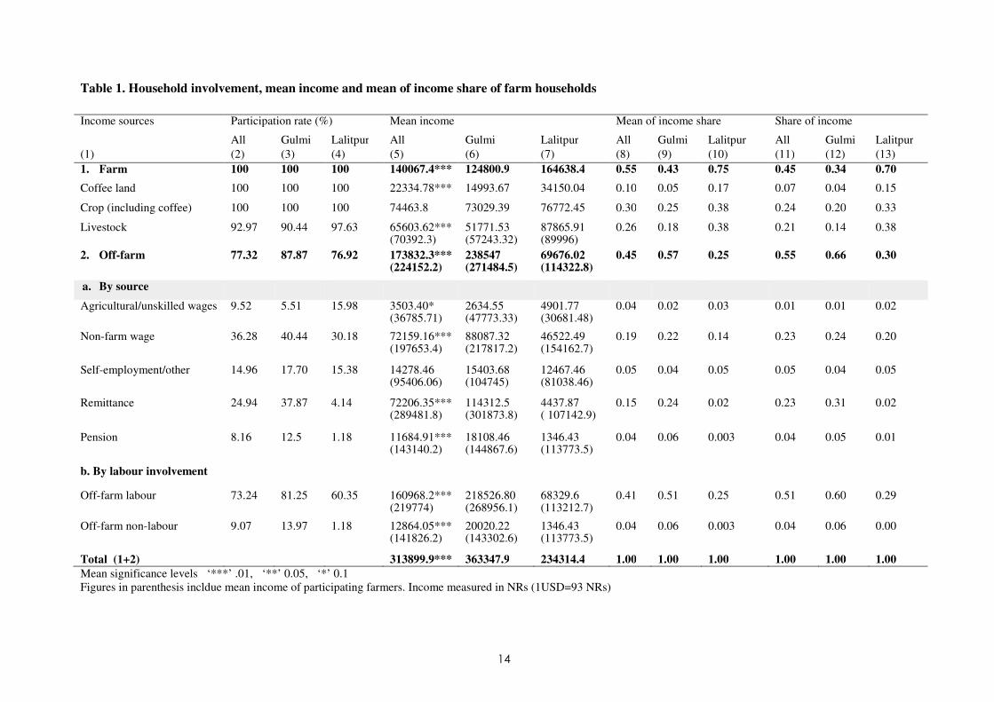
Table 1 presents the summary statistics for household income grouped by farm and off-farm

source. In addition to crop farming, more than 90% households are engaged in livestock

rearing while 77% of households engage in off-farm work. Non-farm wages, remittances and

self-employment are the major off-farm income sources. Households in Gulmi district have a

higher participation in off-farm income sources, particularly in non-farm activities and

remittance than in Lalitpur. Consequently, a larger proportion of households in Lalitpur are

engaged in agricultural or low-wage earning localized activities than in Gulmi where labour

emigration is the principal off-farm income source. Our results corroborate the previous

findings by De Janvry and Sadoulet (2001) and Davis et al. (2010) that households derive

more income from off-farm sources than from farm sources.

Similarly, mean of income share (��) from farm sources (55%) is greater than that from

off-farm sources (45%) (Table 1, columns 8-10), while the opposite is true for the share of

income (��) from farm (45%) and off-farm (55%) sources in total income (Table 3, column

13

11-13). A higher participation in farm activities, a higher mean share of farm income and a

low farm income relative to off-farm sources indicate a subsistence mode of farming

households. A significant proportion of the off-farm income (92.6%) comes from direct and

indirect labour while the rest of the off-farm income (7.4%) have no labour involvements.

Off-farm income is split into overseas and domestic sources. On average, households earn

NRs 80,011 (46%) and NRs 93,821 (54%) from overseas and domestic off-farm sources,

respectively. Further, analysis of participating households show that overseas off-farm

income (NRs 280,040; n=126) is higher than domestic off-farm income (NRs 166,164;

n=249).

14

Table 1. Household involvement, mean income and mean of income share of farm households

Mean significance levels ‘***’ .01, ‘**’ 0.05, ‘*’ 0.1

Figures in parenthesis incldue mean income of participating farmers. Income measured in NRs (1USD=93 NRs)

Income sources Participation rate (%) Mean income Mean of income share Share of income

All Gulmi Lalitpur All Gulmi Lalitpur All Gulmi Lalitpur All Gulmi Lalitpur

(1) (2) (3) (4) (5) (6) (7) (8) (9) (10) (11) (12) (13)

1. Farm

100 100 100 140067.4***

124800.9

164638.4

0.55

0.43

0.75

0.45 0.34 0.70

Coffee land 100 100 100 22334.78***

14993.67

34150.04

0.10 0.05 0.17 0.07 0.04 0.15

Crop (including coffee)

100 100 100 74463.8

73029.39

76772.45

0.30 0.25 0.38 0.24 0.20 0.33

Livestock

92.97 90.44 97.63 65603.62*** (70392.3)

51771.53 (57243.32)

87865.91 (89996)

0.26 0.18 0.38 0.21 0.14 0.38

2. Off-farm

77.32 87.87 76.92 173832.3*** (224152.2)

238547 (271484.5)

69676.02 (114322.8)

0.45 0.57 0.25 0.55 0.66 0.30

a. By source

Agricultural/unskilled wages 9.52 5.51 15.98 3503.40* (36785.71)

2634.55 (47773.33)

4901.77 (30681.48)

0.04 0.02 0.03 0.01 0.01 0.02

Non-farm wage 36.28 40.44 30.18 72159.16*** (197653.4)

88087.32 (217817.2)

46522.49 (154162.7)

0.19 0.22 0.14 0.23 0.24 0.20

Self-employment/other 14.96 17.70 15.38 14278.46 (95406.06)

15403.68 (104745)

12467.46 (81038.46)

0.05 0.04 0.05 0.05 0.04 0.05

Remittance 24.94 37.87 4.14 72206.35*** (289481.8)

114312.5 (301873.8)

4437.87 ( 107142.9)

0.15 0.24 0.02 0.23 0.31 0.02

Pension 8.16 12.5 1.18 11684.91*** (143140.2)

18108.46 (144867.6)

1346.43 (113773.5)

0.04 0.06 0.003 0.04 0.05 0.01

b. By labour involvement

Off-farm labour 73.24 81.25 60.35 160968.2*** (219774)

218526.80 (268956.1)

68329.6 (113212.7)

0.41 0.51 0.25 0.51 0.60 0.29

Off-farm non-labour 9.07 13.97 1.18 12864.05*** (141826.2)

20020.22 (143302.6)

1346.43 (113773.5)

0.04 0.06 0.003 0.04 0.06 0.00

Total (1+2) 313899.9*** 363347.9 234314.4 1.00 1.00 1.00 1.00 1.00 1.00

15

Household’s mean of income share (��) and share of income (��) differ between the districts,

indicating households in Lalitpur receive a higher �� and �� than in Gulmi. Furthermore,

household income differs significantly between the districts for all sources except crops and self-

employment. A higher farm income in Lalitpur than in Gulmi is contrary to our expectations that

the households in Lalitpur, which are close to the capital city Kathmandu, would have more off-

farm income opportunities than the households in Gulmi. The plausible reasons for this result

include a higher dependency of household on farming (Table 1 column 2-4), higher proportion of

land allocated for farming (Lalitpur=0.83; Gulmi=0.54) despite a lower landholding

(Lalitpur=0.76ha; Gulmi=1.01ha) and a higher income and better market access for agricultural

produce (mainly livestock products, vegetable and coffee) in Lalitpur.

Table 2 presents summary statistics of the sources of household income by landholding sizes.

Results show that households’ aggregate participation in off-farm income source increases but

the mean of income share (��) decreases with increased landholding. This indicates low

landholding household’s limited access to remunerative off-farm sources which may be due to

entry barriers such as access to education and household assets. Household’s access to

remittance, a specific form of off-farm income, increases with landholding. There could be two

plausible reasons for increased access to remittances. First, a higher income from foreign

employment and better foreign currency exchange rates motivate household members to

emigrate. Secondly, wealthier households are able to afford better education, which in turn

increases their access to the international labour markets whereas the poorer households are

constrained by a higher transaction cost to enter labour markets such as in Malaysia and other

Middle East countries. Additionally, the income for each source increases with landholding

except for unskilled/agricultural wage as expected. The non-farm wage and farm source specific

mean of shares also increase with landholding.

16

Table2. Household involvement, mean income and mean of income share by landholdings

Income measured in NRs (1USD=93 NRs)

Income sources Participation rate (%) Mean income (NRs) Mean of income share Share of income

≤0.5 ha >0.5 - ≤1 >1 ha ≤0.5 ha >0.5 - ≤1 >1 ha ≤0.5

ha

>0.5 - ≤1 >1 ha ≤0.5 ha >0.5 - ≤1 >1 ha

(1) (2) (3) (4) (5) (6) (7) (8) (9) (10) (11) (12) (13)

Number of FHHs (%) 128

(29.04)

176

(39.90)

137

(31.06)

128

(29.04)

176

(39.90)

137

(31.06)

128

(29.04)

176

(39.90)

137

(31.06)

128

(29.04)

176

(39.90)

137

(31.06)

1. Farm total 100 100 100 106659.3 134951.80 177852.80 0.52 0.56 0.57 0.43 0.45 0.45

Coffee land 100 100 100 17733.05 22976.22 25810.15 0.10 0.10 0.09 0.07 0.08 0.07

Crop (including coffee)

100 100 100 50766.03 70145.91 102151.90 0.25 0.30 0.33 0.20 0.24 0.26

Livestock

92.19 93.75 93.43 55893.23 64805.89 75700.92 0.27 0.26 0.24 0.22 0.22 0.19

2. Off-farm total

81.25 77.84 73.72 143500.4 162029.10 217334.80 0.48 0.44 0.43 0.57 0.55 0.55

a. Off-farm by source

Agricultural/unskilled

wage 14.84 9.66 4.58 5921.88 3076.70 1791.97 0.05 0.02 0.01 0.02 0.01 0.00

Non-farm wage 32.81 32.38 45.25 52892.98 65565.45 98630.44 0.17 0.18 0.23 0.21 0.22 0.25

Remittance 24.22 27.27 29.25 55562.50 75670.45 83306.57 0.15 0.18 0.12 0.22 0.25 0.21

Pension 7.81 6.25 10.94 12324.59 9258.52 14204.38 0.04 0.03 0.03 0.05 0.03 0.04

Self-employment/other 14.84 11.93 18.98 16798.44 8457.95 19401.46 0.06 0.03 0.05 0.07 0.03 0.05

b. By labour

involvement

Off-farm labour 77.34 72.16 70.80 131175.80 152514.90 199663.30 0.43 0.41 0.39 0.52 0.51 0.51

Off-farm non-labour 7.81 7.38 12.40 12324.59 9514.20 17671.53 0.05 0.03 0.41 0.05 0.03 0.04

Household total (1+2) 100 100 100 250159.6 296980.90 395187.60 1.00 1.00 1.00 1.00 1.00 1.00

17

Figure 3 shows how smoothed income share changes in relation to total income ranked by

income level. The off-farm income and its share rise linearly with total income while farm

income follows a smooth pattern with its share dropping down markedly with total income. From

the graph, we can infer that farm income is important for low income earners while off-farm

income is important for enhanced household welfare. Comparing these figures (Figure 4) across

landholdings shows: 1) a lower share of farm income and relatively higher share of off-farm

income for small landholders; and 2) a reverse pattern with farm income share dominating off-

farm income as landholding increases. A comparison of income sources and income shares by

family education (Figure 5) shows that off-farm income share increases at an increasing rate for

better educated households while farm income dominates its share for less educated households.

Figure 3. Farm and off-farm income and their share to household income

Farm income share

Off-farm income share

Off-farm income

Farm income

Income (NRs 10000) Income share

010

20

30

40

50

60

70

80

90

10

0

015

30

45

60

75

90

10

512

0

0 25 50 75 100 125 150Household income (NRs 10000)

18

Figure 4. Farm and off-farm income and their share to household income by landholdings

Figure 5. Farm and off-farm income and their share to household income across education


Farm income share

Farm income

Off-farm income

Income (NRs 10000) Percent share

09

18

27

36

45

54

63

72

04

812

16

20

24

28

32

36

0 .5 1 1.5 2 2.5 3 3.5 4Landholdings (ha)

Farm income share Off-farm income


Farm income

Percent share

08

16

24

32

40

48

56

64

72

80

03

69

12

15

18

21

24

27

0 1 2 3 4 5 6 7 8Family education level

Income (NRs 10000)

Note: family education as defined.

19

Finally, �� from coffee land (7%) shows a marginal contribution to household income. A lower

level of income with less land allocated for coffee may be associated with production (coffee

stem borer and coffee rust) and marketing (uncertain market and low price) risk which is

evidenced by farmers’ past experience in Gulmi. In addition, farmers have to wait until

investment return pays off to allocate more lands for coffee production, although partial return

can be received from non-coffee products from coffee farm. The �� from coffee in Lalitpur is

higher and significantly different (0.01 levels) from Gulmi mainly due to greater land allocation,

better market access and higher farm-gate prices. Figure 6 further shows that income from coffee

increases for the bottom one-third households ranked by income while its share to household

income falls markedly as the household income rises. However, coffee specific income shows a

gradual increase with relatively stable share to the total household income based on landholding

(Figure 7). Furthermore, the �� from coffee land decreases sharply as household education

increases (Figure 8), indicating that coffee farming contributes more income to poor and less

educated households.

Figure 6. Income from coffee land and its share to household income

Income from coffee land

Share of income

Percent share

05

10

15

20

25

0.5

11.5

22.5

3

0 25 50 75 100 125 150Household income (NRs 10000)

Income (NRs 10000)

20

Figure 7. Income from coffee land and its share to household income across landholdings

Figure 8. Income from coffee land and its share to household income by education


Income share

03

69

12

15

0.5

11.5

22.5

33.5

44.5

0 .5 1 1.5 2 2.5 3 3.5 4Land holdings (ha)



Share to household income


Note: education level as defined

04

812

16

20

0.5

11.5

22.5

0 1 2 3 4 5 6 7 8Family education

21

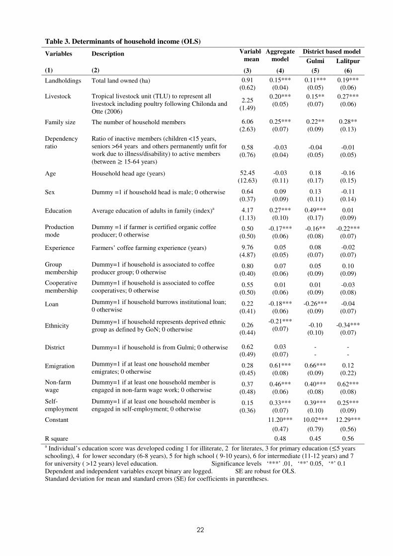
5.2 Determinants of household income

Table 3 presents the results of the analysis of determinants of household income. The coefficients

of the continuous variables reported in Table 3 represent variable-specific income elasticities.

The results show that household income significantly increases with land and livestock holdings,

family size, emigration, participation in non-farm wages and self-employment. Education has a

positive effect on household income in the aggregate model and also in Gulmi district. Certified

coffee production significantly decreases the household income, a result contrary to our

expectation. The negative and significant coefficient for the ethnicity in the aggregate model

indicates that ethnic groups are marginalized in terms of education, landholdings and other

opportunities that further limit their entry to remunerative off-farm income sources. This is

particularly significant in Lalitpur district as evidenced by district based model. The institutional

loans negatively affect income in Gulmi district, indicating high income households are self-

reliant and don’t borrow money from lending institutions. Our results on income determinants

corroborates the earlier findings for education and geographical location in Cambodia (Rahut &

Micevska Scharf 2012), and for education in rural Ghana (Marchetta 2013).

22

Table 3. Determinants of household income (OLS)

Variables Description Variable

mean

Aggregate

model

District based model

Gulmi Lalitpur

(1) (2) (3) (4) (5) (6)

Landholdings Total land owned (ha) 0.91

(0.62)

0.15***

(0.04)

0.11***

(0.05)

0.19***

(0.06)

Livestock

Tropical livestock unit (TLU) to represent all

livestock including poultry following Chilonda and

Otte (2006)

2.25

(1.49)

0.20***

(0.05)

0.15**

(0.07)

0.27***

(0.06)

Family size The number of household members 6.06

(2.63)

0.25***

(0.07)

0.22**

(0.09)

0.28**

(0.13)

Dependency

ratio

Ratio of inactive members (children <15 years,

seniors >64 years and others permanently unfit for

work due to illness/disability) to active members

(between ≥ 15-64 years)

0.58

(0.76)

-0.03

(0.04)

-0.04

(0.05)

-0.01

(0.05)

Age Household head age (years) 52.45

(12.63)

-0.03

(0.11)

0.18

(0.17)

-0.16

(0.15)

Sex Dummy =1 if household head is male; 0 otherwise 0.64

(0.37)

0.09

(0.09)

0.13

(0.11)

-0.11

(0.14)

Education Average education of adults in family (index)a 4.17

(1.13)

0.27***

(0.10)

0.49***

(0.17)

0.01

(0.09)

Production

mode

Dummy =1 if farmer is certified organic coffee

producer; 0 otherwise 0.50

(0.50)

-0.17***

(0.06)

-0.16**

(0.08)

-0.22***

(0.07)

Experience Farmers’ coffee farming experience (years) 9.76

(4.87)

0.05

(0.05)

0.08

(0.07)

-0.02

(0.07)

Group

membership

Dummy=1 if household is associated to coffee

producer group; 0 otherwise 0.80

(0.40)

0.07

(0.06)

0.05

(0.09)

0.10

(0.09)

Cooperative

membership

Dummy=1 if household is associated to coffee

cooperatives; 0 otherwise 0.55

(0.50)

0.01

(0.06)

0.01

(0.09)

-0.03

(0.08)

Loan Dummy=1 if household burrows institutional loan;

0 otherwise 0.22

(0.41)

-0.18***

(0.06)

-0.26***

(0.09)

-0.04

(0.07)

Ethnicity Dummy=1 if household represents deprived ethnic

group as defined by GoN; 0 otherwise 0.26

(0.44)

-0.21***

(0.07)

-0.10

(0.10)

-0.34***

(0.07)

District Dummy=1 if household is from Gulmi; 0 otherwise 0.62

(0.49)

0.03

(0.07)

-

-

-

-

Emigration Dummy=1 if at least one household member

emigrates; 0 otherwise 0.28

(0.45)

0.61***

(0.08)

0.66***

(0.09)

0.12

(0.22)

Non-farm

wage

Dummy=1 if at least one household member is

engaged in non-farm wage work; 0 otherwise 0.37

(0.48)

0.46***

(0.06)

0.40***

(0.08)

0.62***

(0.08)

Self-

employment

Dummy=1 if at least one household member is

engaged in self-employment; 0 otherwise 0.15

(0.36)

0.33***

(0.07)

0.39***

(0.10)

0.25***

(0.09)

Constant 11.20*** 10.02*** 12.29***

(0.47) (0.79) (0.56)

R square 0.48 0.45 0.56 a Individual’s education score was developed coding 1 for illiterate, 2 for literates, 3 for primary education (≤5 years

schooling), 4 for lower secondary (6-8 years), 5 for high school ( 9-10 years), 6 for intermediate (11-12 years) and 7

for university ( >12 years) level education. Significance levels ‘***’ .01, ‘**’ 0.05, ‘*’ 0.1

Dependent and independent variables except binary are logged. SE are robust for OLS.

Standard deviation for mean and standard errors (SE) for coefficients in parentheses.

23

Table 4 shows the OLS and Tobit regression results for disaggregated farm (farm total and coffee

farm) and off-farm (off-farm total, non-farm wage and remittance) incomes respectively. The

total farm income significantly increases with land and livestock holdings, group and cooperative

memberships and self-employment, but it is negatively affected by certified mode of production

and ethnicity. There is also a clear difference in farm incomes between the study districts,

indicating higher (lower) incomes in Lalitpur (Gulmi). Income from coffee farm, including coffee

and non-coffee products, increases significantly with land and livestock holdings, household’s

affiliation with coffee producer group, while such income decreases significantly with family size

and certified mode of production. In a Nicaraguan study, Beuchelt and Zeller (2011) found

organic and fair trade producers receive a lower net income from coffee despite a high farm gate

price and gross margin.

A negative and significant impact of the certified mode of production for farm-based incomes,

particularly coffee land specific income, is surprising. This is in contrary to the broader policy

objective of improving household’s livelihood through the introduction of income generating

cash crops into the farming system. One possible reason for this might be low economies of scale

because of smaller size of coffee farms and smaller share of coffee income to total household

income. Besides, coffee production is labour intensive and the certified producers have to follow

prescribed guidelines, such as no use of chemical fertilizer and pesticides, thus increasing

production costs. In addition, while examining this result closely with the ground reality, it is

apparent that ‘coffee producers’ cooperative union in the district holds authority for certification

and households’ entry and exit from the certification scheme. A lack of two-way trust is observed

among producers, cooperative and traders. More importantly, despite the GoN’s support price for

organic coffee, producers and traders were not honest in their contractual agreement and show

opportunistic behaviour at times to maximise their return going beyond cooperative policy and

norms.

24

Table 4. Determinants of household incomes by sources

Variables Farm income - OLS

model

Off-farm income - Tobit model

Total Coffee farm Total Non-farm

wage

Remittanc

e Landholdings 0.25*** 0.23*** -0.94*** -0.88 -1.24

(0.05) (0.08) (0.33) (1.05) (1.24)

Livestock 0.56*** 0.29*** -0.99** -3.20** -0.34

(0.06) (0.10) (0.40) (1.25) (1.61)

Family size -0.05 -0.33*** 1.06* 9.08*** 7.88***

(0.09) (0.15) (0.57) (2.01) (2.20)

Dependency ratio -0.04 -0.08 -0.02 -0.09 1.19

(0.04) (0.07) (0.30) (0.94) (1.18)

Age -0.15 -0.21 2.78*** 7.22** 5.17

(0.14) (0.22) (0.96) (3.12) (4.15)

Sex 0.13 0.01 -0.57 0.74 -8.66***

(0.08) (0.14) (0.60) (1.99) (2.12)

Education 0.04 0.25 0.64 21.04*** 8.36**

(0.10) (0.17) (0.75) (3.04) (3.32)

Production mode -0.18*** -0.53*** -

(0.06) (0.11) -

Experience -0.01 0.06 -

(0.05) (0.10) -

Group membership 0.18** 0.43*** 0.35 1.00 -0.43

(0.07) (0.12) (0.52) (1.64) (2.06)

Cooperative membership 0.13* 0.23** -0.95** 0.92 -1.14

(0.07) (0.12) (0.47) (1.53) (1.76)

Loan -0.08 -0.03 -1.17** 0.34 0.41

(0.09) (0.13) (0.51) (0.34) (2.15)

Ethnicity -0.30*** 0.00 1.89*** -1.30 0.13

(0.07) (0.12) (0.53) (1.74) (2.09)

District -0.27*** -1.07*** 0.86 3.24* 17.19***

(0.08) (0.13) (0.53) (1.69) (2.63)

Emigration 0.07 -0.19 5.73*** -9.76*** -

(0.08) (0.13) (0.54) (1.74) -

Non-farm wage 0.05 -0.02 6.51*** - -14.23***

(0.06) (0.11) (0.48) - (2.08)

Self-employment 0.13* 0.04 6.07*** -7.48*** -10.41***

(0.07) (0.15) (0.58) (1.97) (2.88)

Constant 11.93*** 10.62*** -9.57** -74.48*** -51.12***

(0.55) (0.93) (4.07) (14.14) (18.27)

R square 0.46 0.40 - - -

Prob>Chi square - - 0 0 0

No. of left censored observations - - 99 281 331

Log likelihood - - -1054.39 -739.97 -521.73

Significance levels ‘***’ .01, ‘**’ 0.05, ‘*’ 0.1 aCoffee farm income includes coffee and non-coffee products.

SE in parentheses and and robust for OLS.

25

Table 4 shows the Tobit model results for the off-farm incomes (total, non-farm wage and

remittance). Total off-farm income decreases significantly with land and livestock holdings,

cooperative membership and institutional loan. Participation in non-farm wages, emigration, self-

employment, household head age, ethnicity and family size are also strongly and positively

associated with the total off-farm income. The negative relationship between landholdings and

off-farm income has also been suggested by previous findings (Barrett et al., 2001; De Janvry &

Sadoulet, 2001; Escobal, 2001).

The non-farm wage income significantly increases with family size, household head age and

educational status while it decreases significantly with emigration, self-employment and livestock

holding. Similarly, remittance significantly increases with family size and education, is lower in

male-headed households, and significantly decreases with participation in non-farm wage and

self-employment. Remittance earning is significantly higher among sample households in Gulmi

compared to Lalitpur, and its share is highly elastic to family size. However, our finding on

higher and significant income by remotely located households from off-farm sectors (non-farm

wage and remittance) is in contrast to the finding by Abdulai and CroleRees (2001) from Mali

where they found that remote areas are less likely to participate in non-cropping sector. So,

emigration of family members is a tendency of large families and households in Gulmi district for

mitigating income risk and wealth accumulation.

The strong association between education and income has important implications for households

and their access to labour markets. Firstly, as the demand for education increases, it increases

labour market access, contributing to household income through increased off-farm income by

shifting the off-farm income line upwards – the line BB’ in Figure 1. Secondly, the strong

correlation between education and income significantly increases the use of hired labour in farm

activities. We use evidence using the mean of the hired labour share (hired labour to total labour

requirement denoted as �̅) in crop activities which increases significantly at .01 levels for

26

households deriving income from non-farm wage (n=161, �̅=0.26) and remittance (n=110,

�̅ =0.29) compared to those not deriving income from non-farm wage (n=280, �̅=0.20) and

remittance (n=331, �̅ =0.20). Two parallel lines running down through B and E (Figure 1) show

household labour substitution by hired labour to meet farm labour requirements.

6. Conclusion and policy implications

Our findings suggest that subsistence farming households receive a higher share of income from

off-farm sources than from farming. Of the off-farm sources, domestic non-farm wage and

remittance through international labour markets are major sources to increase household income.

Emigration, households’ participation in non-farm wages, self-employment, education, family

size, livestock and landholdings are the significant determinants of household income, but

landholding and education have a particular significance for remunerative off-farm income

through direct and indirect labour use. Thus, education is an important precursor to increasing

income and reducing dependence on resource-poor farms. A strong association between

education and labour market income increases the demand for education and substitute the farm

labour need by hired labour.

Despite a lower income contribution from coffee enterprise, income from coffee farms is higher

for poor and less educated households and for those who live close to market centres (Lalitpur).

The finding that small contribution of coffee enterprise to household income and negative impact

on income through organic mode of production are contrary to the presumption that income

generating cash crops help improve the living standard of farming households. But our results

suggest that household income is influenced by household assets and exposure to education, thus

household context specific.

27

This research contributes to the debate in development economics in addressing the subsistence

households’ income strategy through an analysis of a commodity specific development policy.

Our result are consistent with De Janvry and Sadoulet (2001) who emphasize the role of

education in generating higher payoff from off-farm labour market. Increasing access to off-farm

income therefore becomes important strategy to enhance welfare of farming households who are

faced with limited land but surplus labour resource. Thus, the promotion of organic coffee in

Nepal or in similar context elsewhere should be targeted and focused on low income and less

educated households, who are educationally marginalized and unable to meet the entry

requirements for labour market access, thus derive a relatively higher proportion of income from

such agricultural interventions.

References

Abdulai, A & CroleRees, A 2001, 'Determinants of income diversification amongst rural

households in southern Mali', Food Policy, vol. 26, pp. 437-452.

Angrist, JD & Krueger, AB 1991, 'Does compulsory school attendance affect schooling and

earnings?', The Quarterly Journal of Economics, vol. 106, no. 4, pp. 979-1014.

Barnum, HN & Squire, L 1979, A model of an agricultural household:Theory and Evidence.

World Bank Staff Occasional Papers. No 27. Johns Hopkins University Press. Baltimore

and London.

Barrett, CB, Reardon, T & Webb, P 2001, 'Nonfarm income diversification and household

livelihood strategies in rural Africa:concepts, dynamics, and policy implications', Food

Policy, vol. 26, pp. 315-331.

Battese, GE 1997, 'A note on the estimation of Cobb-Douglas production function when some

explanatory variables have zero values', Journal of Agricultural Economics, vol. 48, no.

1-3, pp. 250-252.

Becker, GS 1965, 'A theory of the allocation of time.', Economic Journal, vol. 75, no. 299, pp.

493-517.

Beuchelt, TD & Zeller, M 2011, 'Profits and poverty: Certification's troubled link for Nicaragua's

organic and fairtrade coffee producers', Ecological Economics, vol. 70, no. 7, pp. 1316-

1324.

28

Bhandari, BS & Grant, M 2007, 'Analysis of livelihood security: A case study in the Kali-Khola

watershed of Nepal', Journal of Environmental Management, vol. 85, no. 1, pp. 17-26.

Brown, S & Shrestha, B 2000, 'Market-driven land-use dynamics in the middle mountains of

Nepal', Journal of Environmental Management, vol. 59, no. 3, pp. 217-225.

Card, D 1999, 'The causal effect of education on earnings', in Handbook of Labor Economics,

vol. Volume 3, Part A, eds CA Orley & C David, Elsevier, pp. 1801-1863.

Card, D 2001, 'Estmating the return to schooling:Progress on some persistent econometric

problems', Econometrica, vol. 69, no. 5, pp. 1127-1160.

CBS 2011, National population and housing census (national report), Central Bureau of

Statistics, Kathmandu, Nepal.

Chilonda, P & Otte, J 2006, Indicators to monitor trends in livestock production at national,

regional and inernational levels. Livestock Research for Rural Development 18(8) Article

117. [ Retrieved May 3, 2014, from http://www.lrrd.org/lrrd18/8/chil18117.htm].

Davis, B, Paul, W, Gero, C, Katia, K, Esteban, Q, Alberto, Z, Kostas, E, Carlo, A & Stefania, D

2010, 'A cross country comparison of rural income generating activities', World

Development, vol. 38, no. 1, pp. 48-63.

Davis, B, Winters, P, Reardon, T & Stamoulis, K 2009, 'Rural nonfarm employment and farming:

household-level linkages', Agricultural Economics, vol. 40, no. 2, pp. 119-123.

De Janvry, A & Sadoulet, E 1996, Household modeling for the design of poverty alleviatio

strategies [Working paper No 787], University of California at Berkeley, Berkeley, USA.

De Janvry, A & Sadoulet, E 2001, 'Income strategies among rural households in Mexico:The role

of off-farm activities', World Development, vol. 29, no. 3, pp. 467-480.

Deininger, K & Olinto, P 2001, 'Rural nonfarm employment and income diversification in

Colombia', World Development, vol. 29, no. 3, pp. 455-465.

Devendra, C & Thomas, D 2002, 'Smallholder farming systems in Asia', Agricultural Systems,

vol. 71, no. 1–2, pp. 17-25. [2002/2//].

Dewbre, J & Mishra, AK 2002, Farm household incomes and US government program payments,

No 19780, 2002, Annual meeting, July 28-31, Long Beach, CA, American Agricultural

Economics Association.

Dickson, M & Harmon, C 2011, 'Economic returns to education: What we know, what we don’t

know, and where we are going—Some brief pointers', Economics of Education Review,

vol. 30, no. 6, pp. 1118-1122.

DoFE 2014, Labour migration for employment:A status report for Nepal 2013/2014, Department

of Foreign Employment. Ministry of Labour and Employment. Government of Nepal,

Kathmandu.

Escobal, J 2001, 'The determinants of non-farm income diversification in rural Peru', World

Development, vol. 29, no. 3, pp. 497-508.

29

Fan, S & Chan-Kang, C 2005, 'Is small beautiful? Farm size, productivity, and poverty in Asian

agriculture', Agricultural Economics, vol. 32, pp. 135-146.

FAO 1998, Rural non-farm income in developing countries, Food and Agriculture Organizations,

Rome, Italy.

Greene, WH 2003, Econometric Analysis, 5 edn, Prentince Hall, New York, USA.

Gujarati, DN & Porter, DC 2009, Basic econometrics (fifth edition), McGraw-Hill /Irwin,

NewYork, USA.

Hagen, E 2008, Development of coffee production in Nepal Masters Thesis thesis, University of

Agder. Norway.

Huang, J, Wu, Y & Rozelle, S 2009, 'Moving off the farm and intensifying agricultural

production in Shandong: a case study of rural labor market linkages in China',

Agricultural Economics, vol. 40, no. 2, pp. 203-218.

Jean-Francois, M, Mueller, V & Sebastian, A 2014, Environmental migration and labor markets

in Nepal. IFPRI discussion paper 01364. August 2014, International Food Policy

Research Institute, Washington, DC.

Kattel, RR, Jena, P & Grote, U 2009, 'The impact of coffee production on Nepali smallholders in

the value chain ', Biophysical and Socio-Economic Frame Conditions for the Sustainable

Management of Natural Resources pp. 1-5.

Kayastha, P, Rauniyar, GP & Parker, WJ 1998, Determinants of off-farm employment in eastern

rural Nepal, Massey University, New Zealand.

Lee, JE 1965, 'Allocating Farm Resources between Farm and Nonfarm Uses', Journal of Farm

Economics, vol. 47, no. 1, pp. 83-92.

MacKinnon, JG & White, H 1985, 'Some heteroskedastic-consistent covariance matrix estimators

with improved finite sample properties', Journal of Econometrics, vol. 29, no. 29, pp.

305-325.

Maharjan, A, Bauer, S & Knerr, B 2012, 'International migration, remitances and subsistence

farming:Evidence from Nepal.', International Migration vol. 51, no. 3, pp. 1-15.

Marcel, F & Shilpi, F 2003, 'The spatial division of labour in Nepal', The Journal of Development

Studies, vol. 39, no. 6, pp. 23-66.

Marchetta, F 2013, 'Migration and nonfarm act vities as income diversification strategies: The

case of Northern Ghana', Canadian Journal of Development Studies, vol. 34, no. 1, pp. 1-

21.

MoAD 2014, Statistical information on Nepalese agriculture 2013/2014, Ministry of Agricultural

Development, Kathmandu, Nepal.

Poudel, KL 2012, Farm management economics of organic coffee in rural hill of Nepal, LAP

LAMBERT Academic Publishing GmbH & Co. KG, Saarbrucken, Germany.

Rahut, DB & Micevska Scharf, M 2012, 'Non-farm employment and incomes in rural Cambodia',

Asian-Pacific Economic Literature, vol. 26, no. 2, pp. 54-71.

30

Reardon, T 1997, 'Using evidence of household income diversification to inform study of the

rural nonfarm labor market in Africa', World Development vol. 25, no. 5, pp. 735-748.

Regmi, G & Tisdell, C 2002, 'Remitting Behaviour of Nepalese Rural-to-Urban Migrants:

Implications for Theory and Policy', The Journal of Development Studies, vol. 38, no. 3,

pp. 76-94.

Schmitt, GH 1988, 'What do agricultural income and productivity measuments really mean?',

Agricultural Economics, vol. 2, pp. 139-157.

Senadza, B 2012, 'Non-farm income diversification in rural Ghana: Patterns and determinants',

African Development Review/Revue Africaine de Developpement, vol. 24, no. 3, pp. 233-

244.

Singh, I, Squire, L & Strauss, J 1986, 'A survey of agricultural household models: Recent

findings and policy implications', The World Bank Economic Review, vol. 1, no. 1, pp.

149-179.

Weinberger, K & Lumpkin, TA 2007, 'Diversification into Horticulture and Poverty Reduction:

A Research Agenda', World Development, vol. 35, no. 8, pp. 1464-1480.

Winters, P, Essam, T, Zezza, A, Davis, B & Carletto, C 2010, 'Patterns of rural development: A

cross-country comparison using microeconomic data', Journal of Agricultural Economics,

vol. 61, no. 3, pp. 628-651.

wp1508 sharma et al income diversification of coffee...

Documents