worst-case value-at-risk of non-linear portfolios · worst-case value-at-risk of non-linear...
TRANSCRIPT

Worst-Case Value-at-Risk of Non-Linear Portfolios
Steve Zymler∗, Daniel Kuhn and Berç Rustem
Department of ComputingImperial College of Science, Technology and Medicine
180 Queen’s Gate, London SW7 2AZ, UK.
June 21, 2012
Abstract
Portfolio optimization problems involving Value-at-Risk (VaR) are often computationallyintractable and require complete information about the return distribution of the portfo-lio constituents, which is rarely available in practice. These difficulties are compoundedwhen the portfolio contains derivatives. We develop two tractable conservative approxi-mations for the VaR of a derivative portfolio by evaluating the worst-case VaR over allreturn distributions of the derivative underliers with given first- and second-order moments.The derivative returns are modelled as convex piecewise linear or—by using a delta-gammaapproximation—as (possibly non-convex) quadratic functions of the returns of the derivativeunderliers. These models lead to newWorst-Case Polyhedral VaR (WPVaR) andWorst-CaseQuadratic VaR (WQVaR) approximations, respectively. WPVaR serves as a VaR approxi-mation for portfolios containing long positions in European options expiring at the end ofthe investment horizon, whereas WQVaR is suitable for portfolios containing long and/orshort positions in European and/or exotic options expiring beyond the investment horizon.We prove that—unlike VaR that may discourage diversification—WPVaR and WQVaR arein fact coherent risk measures. We also reveal connections to robust portfolio optimization.
Key words. Value-at-Risk, Derivatives, Robust Optimization, Second-Order Cone Pro-gramming, Semidefinite Programming
1 Introduction
Investors face the challenging problem of how to distribute their current wealth over a setof available assets with the goal to earn the highest possible future wealth. One of the firstmathematical models for this problem was formulated by Markowitz [16], who observed that aprudent investor does not aim solely at maximizing the expected return of an investment, butalso at minimizing its risk. In the Markowitz model, the risk of a portfolio is measured by thevariance of the portfolio return.
Although mean-variance optimization is appropriate when the asset returns are symmetri-cally distributed, it is known to result in counterintuitive asset allocations when the portfolio
∗Corresponding author: [email protected]
1
return is skewed. This shortcoming triggered extensive research on downside risk measures. Dueto its intuitive appeal and since its use is enforced by financial regulators, Value-at-Risk (VaR)remains the most popular downside risk measure [14]. The VaR at level ε is defined as the least(1− ε)-quantile of the portfolio loss distribution.
Despite its popularity, VaR lacks some desirable theoretical properties. Firstly, VaR isknown to be a non-convex risk measure. As a result, VaR optimization problems usually arecomputationally intractable. In fact, they belong to the class of chance-constrained stochasticprograms, which are notoriously difficult to solve. Secondly, VaR fails to satisfy the subadditivityproperty of coherent risk measures [3]. Thus, the VaR of a portfolio can exceed the weightedsum of the VaRs of its constituents. In other words, VaR may penalize diversification. Thirdly,the computation of VaR requires precise knowledge of the joint probability distribution of theasset returns, which is rarely available in practice.
A typical investor may know the first- and second-order moments of the asset returns but isunlikely to have complete information about their distribution. Therefore, El Ghaoui et al. [11]propose to maximize the VaR of a given portfolio over all asset return distributions consistentwith the known moments. The resulting Worst-Case VaR (WVaR) represents a conservative(that is, pessimistic) approximation for the true (unknown) portfolio VaR. In contrast to VaR,WVaR represents a convex function of the portfolio weights and can be optimized efficiently bysolving a tractable second-order cone program. El Ghaoui et al. [11] also disclose an interestingconnection to robust optimization [5, 6, 23]: WVaR coincides with the worst-case portfolio losswhen the asset returns are confined to an ellipsoidal uncertainty set determined through theknown means and covariances.
In this paper we study portfolios containing derivatives, the most prominent examples ofwhich are European call and put options. Sophisticated investors frequently enrich their portfo-lios with derivative products, be it for hedging and risk management or speculative purposes. Inthe presence of derivatives, WVaR still constitutes a tractable conservative approximation for thetrue portfolio VaR. However, it tends to be over-pessimistic and thus may result in undesirableportfolio allocations. The main reasons for the inadequacy of WVaR are the following.• The calculation of WVaR requires the first- and second-order moments of the derivative returns
as an input. These moments are difficult or (in the case of exotic options) almost impossibleto estimate due to scarcity of time series data.
• WVaR disregards perfect dependencies between the derivative returns and the underlyingasset returns. These (typically non-linear) dependencies are known in practice as they canbe inferred from contractual specifications (payoff functions) or option pricing models. Notethat the covariance matrix of the asset returns, which is supplied to the WVaR model, failsto capture non-linear dependencies among the asset returns, and therefore WVaR tends toseverely overestimate the true VaR of a portfolio containing derivatives.
Recall that WVaR can be calculated as the optimal value of a robust optimization problemwith an ellipsoidal uncertainty set, which is highly symmetric. This symmetry hints at theinadequacy of WVaR from a geometrical viewpoint. An intuitively appealing uncertainty set
2
should be asymmetric to reflect the skewness of the derivative returns. Recently, Natarajan etal. [18] included asymmetric distributional information into the WVaR optimization in order toobtain a tighter approximation of VaR. However, their model requires forward- and backward-deviation measures as an input, which are difficult to estimate for derivatives. In contrast,reliable information about the functional relationships between the returns of the derivativesand their underlying assets is readily available.
In this paper we develop new Worst-Case VaR models which explicitly account for perfectnon-linear dependencies between the asset returns. We first introduce the Worst-Case Polyhe-dral VaR (WPVaR), which provides a conservative approximation for the VaR of a portfoliocontaining European-style options expiring at the end of the investment horizon. In this sit-uation, the option returns constitute convex piecewise-linear functions of the underlying assetreturns. WPVaR evaluates the worst-case VaR over all asset return distributions consistentwith the given first- and second-order moments of the option underliers and the piecewise linearrelation between the asset returns. Under a no short-sales restriction on the options, we are ableto formulate WPVaR optimization as a convex second-order cone program, which can be solvedefficiently [2]. We also establish the equivalence of the WPVaR model to a robust optimizationmodel described in [29].
Next, we introduce the Worst-Case Quadratic VaR (WQVaR) which approximates the VaRof a portfolio containing long and/or short positions in plain vanilla and/or exotic optionswith arbitrary maturity dates. In contrast to WPVaR, WQVaR assumes that the derivativereturns are representable as (possibly non-convex) quadratic functions of the underlying assetreturns. This can always be enforced by invoking a delta-gamma approximation, that is, asecond-order Taylor approximation of the portfolio return. The delta-gamma approximation ispopular in many branches of finance and is accurate for short investment periods. Moreover, ithas been used extensively for VaR estimation, see, e.g., the surveys by Jaschke [13] and Minaand Ulmer [17]. However, to the best of our knowledge, the delta-gamma approximation hasnever been used in a VaR optimization model. We define WQVaR as the worst-case VaR overall asset return distributions consistent with the known first- and second-order moments of theoption underliers and the given quadratic relation between the asset returns. WQVaR providesa tight conservative approximation for the true portfolio VaR if the delta-gamma approximationis accurate. We show that WQVaR optimization can be formulated as a convex semidefiniteprogram, which can be solved efficiently [25], and we establish a connection to a new robustoptimization problem.
In the aftermath of the financial crisis in 2008 VaR has been heavily criticized for failing tosatisfy the subadditivity property of coherent risk measures, therefore occasionally discouragingdiversification. One of the main insights of this work is that the WVaR by El Ghaoui et al.[11] as well as the new WPVaR and WQVaR measures proposed here are in fact coherent riskmeasures in the sense of Artzner et al. [3]. This will be established by proving that WPVaR(WQVaR) coincides with the worst-case Conditional Value-at-Risk of the underlying polyhedral(quadratic) loss function.
3
The main contributions of this paper can be summarized as follows:
(1) We generalize the WVaR model [11] to explicitly account for the non-linear relationshipsbetween the derivative returns and the underlying asset returns. To this end, we develop theWPVaR and WQVaR models as described above. We show that in the absence of derivativesboth models reduce to the WVaR model. Moreover, we formulate WPVaR optimization asa second-order cone program and WQVaR optimization as a semidefinite program. Bothmodels are polynomial-time solvable.
(2) We show that both the WPVaR and the WQVaR models have equivalent reformulationsas robust optimization problems. We explicitly construct the associated uncertainty setswhich are, unlike conventional ellipsoidal uncertainty sets, asymmetrically oriented aroundthe mean values of the asset returns. This asymmetry is caused by the non-linear dependenceof the derivative returns on their underlying asset returns. Simple examples illustrate thatthe new models may approximate the true portfolio VaR significantly better than WVaR inthe presence of derivatives.
(3) We establish that WPVaR (WQVaR) coincides with the Worst-Case Conditional Value-at-Risk of the underlying polyhedral (quadratic) loss function, and we demonstrate thatWPVaR and WQVaR represent coherent risk measures in the sense of Artzner et al. [3].
Notation. We use lower-case bold face letters to denote vectors and upper-case bold faceletters to denote matrices. The space of symmetric matrices of dimension n is denoted by Sn.For any two matrices X,Y ∈ Sn, we let 〈X,Y〉 = Tr(XY) be the trace scalar product, while therelation X < Y (X Y) implies that X−Y is positive semidefinite (positive definite). Randomvariables are always represented by symbols with tildes, while their realizations are denoted bythe same symbols without tildes. Unless stated otherwise, equations involving random variablesare assumed to hold almost surely. In the case of distributional ambiguity, the equations holdalmost surely with respect to each distribution under consideration.
2 Worst-Case Value-at-Risk Optimization
Consider a market consisting of m assets such as equities, bonds, and currencies. We denote thepresent as time t = 0 and the end of the investment horizon as t = T . A portfolio is characterizedby a vector of asset weights w ∈ Rm, whose elements add up to 1. The component wi denotesthe percentage of total wealth which is invested in the ith asset at time t = 0. Furthermore, rdenotes the Rm-valued random vector of relative assets returns over the investment horizon. Bydefinition, an investor will receive 1 + ri dollars at time T for every dollar invested in asset i attime 0. The return of a given portfolio w over the investment period is thus given by the randomvariable rp = wT r. Loosely speaking, we aim at finding an allocation vector w which entails ahigh portfolio return, whilst keeping the associated risk at an acceptable level. Depending onhow risk is defined, we end up with different portfolio optimization models.
Arguably one of the most popular measures of risk is the Value-at-Risk (VaR). The VaR at
4
level ε is defined as the (1 − ε)-percentile of the portfolio loss distribution, where ε is typicallychosen as 1% or 5%. Put differently, VaRε(w) is defined as the smallest real number γ with theproperty that −wT r exceeds γ with a probability not larger than ε, that is,
VaRε(w) = minγ : Pγ ≤ −wT r ≤ ε
, (1)
where P denotes the distribution of the asset returns r.In this paper we investigate portfolio optimization problems of the type
minimizew∈Rm
VaRε(w)
subject to w ∈ W,(2)
where W ⊆ Rm denotes the set of admissible portfolios. The inclusion w ∈ W usually impliesthe budget constraint wTe = 1 (where e denotes the vector of 1s). Optionally, the set Wmay account for bounds on the allocation vector w and/or a constraint enforcing a minimumexpected portfolio return. In this paper we only require that W must be a convex polyhedron.
By using (1), the VaR optimization model (2) can be reformulated as
minimizew∈Rm,γ∈R
γ
subject to Pγ +wT r ≥ 0 ≥ 1− ε
w ∈ W,
(3)
which constitutes a chance-constrained stochastic program. Optimization problems of this kindare usually difficult to solve since they tend to have non-convex or even disconnected feasiblesets. Furthermore, the evaluation of the chance constraint requires precise knowledge of theprobability distribution of the asset returns, which is rarely available in practice.
2.1 Two Analytical Approximations of Value-at-Risk
In order to overcome the computational difficulties and to account for the lack of knowledge aboutthe distribution of the asset returns, the objective function in (2) must usually be approximated.Most existing approximation techniques fall into one of two main categories: non-parametricapproaches which approximate the asset return distribution by a discrete (sampled or empirical)distribution and parametric approaches which approximate the asset return distribution by thebest fitting member of a parametric family of continuous distributions. We now give a briefoverview of two analytical VaR approximation schemes that are of particular relevance for ourpurposes.
Both in the financial industry as well as in the academic literature, it is frequently assumedthat the asset returns r are governed by a Gaussian distribution with given mean vector µr ∈ Rm
and covariance matrix Σr ∈ Sm. This assumption has the advantage that the VaR can be
5
calculated analytically as
VaRε(w) = −µTrw − Φ−1(ε)√wTΣrw, (4)
where Φ is the standard normal distribution function. This model is sometimes referred to asNormal VaR (see, e.g., [18]). In practice, the distribution of the asset returns often fails to beGaussian. In these cases, (4) can still be used as an approximation. However, it may lead togross underestimation of the actual portfolio VaR when the true portfolio return distribution isleptokurtic or heavily skewed, as is the case for portfolios containing options.
To avoid unduly optimistic risk assessments, El Ghaoui et al. [11] suggest a conservative(that is, pessimistic) approximation for VaR under the assumption that only the mean valuesand covariance matrix of the asset returns are known. Let Pr be the set of all probabilitydistributions on Rm with mean value µr and covariance matrix Σr. We emphasize that Prcontains also distributions which exhibit considerable skewness, so long as they match the givenmean vector and covariance matrix. TheWorst-Case Value-at-Risk for portfoliow is now definedas
WVaRε(w) = min
γ : sup
P∈PrPγ ≤ −wT r ≤ ε
. (5)
El Ghaoui et al. demonstrate that WVaR has the closed form expression
WVaRε(w) = −µTrw + κ(ε)√wTΣrw, (6)
where κ(ε) =√
(1− ε)/ε. WVaR represents a tight approximation for VaR in the sense thatthere exists a worst-case distribution P∗ ∈ Pr such that VaR with respect to P∗ is equal toWVaR.
When using WVaR instead of VaR as a risk measure, we end up with the portfolio optimiza-tion problem
minimizew∈Rm
− µTrw + κ(ε)∥∥∥Σ1/2
r w∥∥∥2
subject to w ∈ W,(7)
which represents a second-order cone program that is amenable to efficient numerical solutionprocedures.
2.2 Robust Optimization Perspective on Worst-Case VaR
Consider the following uncertain linear program.
minimizew∈Rm,γ∈R
γ
subject to γ +wT r ≥ 0
w ∈ W
(8)
6

Since the asset return vector is uncertain, this model essentially represents a whole family ofoptimization problems, one for each possible realization of r. Therefore, (8) fails to provide aunique implementable investment decision. One way to disambiguate this model is to requirethat the explicit inequality constraint in (8) is satisfied with a given probability. By usingthis approach, we recover the chance-constrained stochastic program (3). Robust optimization[5, 4, 7] pursues a different approach to disambiguate the model. The idea is to select a decisionwhich is optimal with respect to the worst-case realization of r within a prescribed uncertaintyset U . This set may cover only a subset of all possible realizations of r and is chosen by themodeller. The robust counterpart of problem (8) is then defined as
minimizew∈Rm,γ∈R
γ
subject to γ +wTr ≥ 0 ∀r ∈ U
w ∈ W.
(9)
The shape of the uncertainty set U should reflect the modeller’s knowledge about the assetreturn distribution, e.g., full or partial information about the support and certain moments ofthe random vector r. Moreover, the size of U determines the degree to which the user wantsto safeguard feasibility of the corresponding explicit inequality constraint. The semi-infiniteconstraint in the robust counterpart (9) is therefore closely related to the chance constraintin the stochastic program (3). For a large class of convex uncertainty sets, the semi-infiniteconstraint in the robust counterpart can be reformulated in terms of a small number of tractable(i.e., linear, second-order conic, or semidefinite) constraints [5, 6].
An uncertainty set that enjoys wide popularity in the robust optimization literature is theellipsoidal set,
U = r ∈ Rm : (r − µr)TΣ−1r (r − µr) ≤ δ2,
which is defined in terms of the mean vector µr and covariance matrix Σr of the asset returnsas well as a size parameter δ. By conic duality it can be shown that the following equivalenceholds for any fixed (w, γ) ∈ W × R.
γ +wTr ≥ 0 ∀r ∈ U ⇐⇒ −µTrw + δ∥∥∥Σ1/2
r w∥∥∥2≤ γ (10)
Problem (9) can therefore be reformulated as the following second-order cone program.
minimizew∈Rm
− µTrw + δ∥∥∥Σ1/2
r w∥∥∥2
subject to w ∈ W(11)
By comparing (7) and (11), El Ghaoui et al. [11] noticed that optimizing WVaR at level ε isequivalent to solving the robust optimization problem (9) under an ellipsoidal uncertainty setwith size parameter δ = κ(ε), see also Natarajan et al. [18]. This uncertainty set will henceforthbe denoted by Uε.
7
In this paper we extend the WVaR model (6) and the equivalent robust optimizationmodel (9) to situations in which there are non-linear relationships between the asset returns, asis the case in the presence of derivatives.
3 Worst-Case VaR for Derivative Portfolios
From now on assume that the market consists of n ≤ m basic assets and m − n derivatives.We partition the asset return vector as r = (ξ, η), where the Rn-valued random vector ξ andRm−n-valued random vector η denote the basic asset returns and derivative returns, respectively.
To approximate the VaR of some portfolio w ∈ W containing derivatives, one can princi-pally still use the WVaR model (6), which has the advantage of computational tractability andaccounts for the absence of distributional information beyond first- and second-order moments.However, WVaR is not a suitable approximation for VaR in the presence of derivatives due tothe following reasons.
The first- and second-order moments of the derivative returns, which must be supplied to theWVaR model, are difficult to estimate reliably from historical data, see, e.g., [10]. Note that themoments of the basic assets’ returns (i.e., stocks and bonds etc.) can usually be estimated moreaccurately due to the availability of longer historical time series. However, even if the means andcovariances of the derivative returns were precisely known, WVaR would still provide a poorapproximation of the actual portfolio VaR because it disregards known perfect dependenciesbetween the derivative returns and their underlying asset returns. In fact, the returns of thederivatives are uniquely determined by the returns of the underlying assets, that is, there existsa (typically non-linear) measurable function f : Rn → Rm such that r = f(ξ).1 Put differently,the derivatives introduce no new uncertainties in the market; their returns are uncertain onlybecause the underlying asset returns are uncertain. The function f can usually be inferredreliably from contractual specifications (payoff functions) or pricing models of the derivatives.
In summary, WVaR provides a conservative approximation to the actual VaR. However, itrelies on first- and second-order moments of the derivative returns, which are difficult to ob-tain in practice, and disregards the perfect dependencies captured by the function f , which aretypically known. When f is non-linear, WVaR tends to severely overestimate the actual VaRsince the covariance matrix Σr accounts only for linear dependencies. The robust optimizationperspective on WVaR manifests this drawback geometrically. Recall that the ellipsoidal uncer-tainty set Uε introduced in Section 2.2 is symmetrically oriented around the mean vector µr. Ifthe underlying assets of the derivatives have approximately symmetrically distributed returns,then the derivative returns are heavily skewed. An ellipsoidal uncertainty set fails to capturethis asymmetry. This geometric argument supports our conjecture that WVaR provides a poor(over-pessimistic) VaR estimate when the portfolio contains derivatives.
In the remainder of the paper we assume to know the first- and second-order moments ofthe basic asset returns as well as the function f , which captures the non-linear dependencies
1For ease of exposition, we assume that the returns of the derivative underliers are the only risk factorsdetermining the option returns.
8
between the basic asset and derivative returns. In contrast, we assume that the moments of thederivative returns are unknown. In the next sections we derive generic Worst-Case Value-at-Risk models that explicitly account for non-linear (piecewise linear or quadratic) relationshipsbetween the asset returns. These new models provide tighter approximations for the actualVaR of portfolios containing derivatives than the WVaR model, which relies solely on momentinformation. Below, we will always denote the mean vector and the covariance matrix of thebasic asset returns by µ and Σ, respectively. Without loss of generality we assume that Σ isstrictly positive definite.
4 Worst-Case Polyhedral VaR Optimization
In this section we describe a Worst-Case VaR model that explicitly accounts for piecewise linearrelationships between option returns and their underlying asset returns. We show that thismodel can be cast as a tractable second-order cone program and establish its equivalence to arobust optimization model that admits an intuitive interpretation.
4.1 Piecewise Linear Portfolio Model
We now assume that the m − n derivatives in the market are European-style call and/or putoptions derived from the basic assets. All these options are assumed to mature at the end ofthe investment horizon, that is, at time T . For ease of exposition, we partition the allocationvector as w = (wξ,wη), where wξ ∈ Rn and wη ∈ Rm−n denote the percentage allocations inthe basic assets and options, respectively. In this section we forbid short-sales of options, thatis, we assume that the inclusion w ∈ W implies wη ≥ 0. Recall that the set W of admissibleportfolios was assumed to be a convex polyhedron.
We now derive an explicit representation for f by using the known payoff functions of thebasic assets as well as the European call and put options. Since the first n components of rrepresent the basic asset returns ξ, we have fj(ξ) = ξj for j = 1, . . . , n. Next, we investigate theoption returns rj for j = n + 1, . . . ,m. Let asset j be a call option with strike price kj on thebasic asset i, and denote the return and the initial price of the option by rj and cj , respectively.If si denotes the initial price of asset i, then its end-of-period price amounts to si(1 + ξi). Wecan now explicitly express the return rj as a convex piecewise linear function of ξi,
fj(ξ) =1
cjmax
0, si(1 + ξi)− kj
− 1
= max−1, aj + bj ξi − 1
, where aj =
si − kjcj
and bj =sicj. (12a)
Similarly, if asset j is a put option with price pj and strike price kj on the basic asset i, then itsreturn rj is representable as a different convex piecewise linear function,
fj(ξ) = max−1, aj + bj ξi − 1
, where aj =
kj − sipj
and bj = − sipj. (12b)
9

Using the above notation, we can write the vector of asset returns r compactly as
r = f(ξ) =
(ξ
max−e,a+ Bξ − e
) , (13)
where a ∈ Rm−n, B ∈ R(m−n)×n are known constants determined through (12a) and (12b),e ∈ Rm−n is the vector of 1s, and ‘max’ denotes the component-wise maximization operator.Thus, the return rp of some portfolio w ∈ W can be expressed as
rp = wT r = (wξ)T ξ + (wη)T η
= wT f(ξ) = (wξ)T ξ + (wη)T max−e,a+ Bξ − e
. (14)
4.2 Worst-Case Polyhedral VaR Model
For any portfolio w ∈ W, we define the Worst-Case Polyhedral VaR (WPVaR) as
WPVaRε(w) = min
γ : sup
P∈PPγ ≤ −wT f(ξ)
≤ ε
(15)
= min
γ : sup
P∈PPγ ≤ −(wξ)T ξ − (wη)T max
−e,a+ Bξ − e
≤ ε,
where P denotes the set of all probability distributions of the basic asset returns ξ with agiven mean vector µ and covariance matrix Σ. WPVaR provides an accurate conservativeapproximation for the VaR of a portfolio whose return constitutes a convex piecewise linear(i.e., polyhedral) function of the basic asset returns. We now demonstrate that WPVaR can beevaluated efficiently as the optimal value of a tractable semidefinite program (SDP).
Theorem 4.1 The WPVaR of a fixed portfolio w ∈ W can be expressed as
WPVaRε(w) = inf γ
s. t. M ∈ Sn+1, y ∈ Rm−n, τ ∈ R, γ ∈ R
〈Ω,M〉 ≤ τε, M < 0, τ ≥ 0, 0 ≤ y ≤ wη
M +
[0 wξ + BTy
(wξ + BTy)T −τ + 2(γ + yTa− eTwη)
]< 0,
(16)
where
Ω =
[Σ + µµT µ
µT 1
](17)
is the second-order moment matrix of ξ.
Proof: See Appendix B.
Even though (16) constitutes a tractable SDP that enables us to compute the WPVaR ofa given portfolio w ∈ W in polynomial time, it would be desirable to obtain an equivalent
10

second-order cone program (SOCP) because SOCPs exhibit better scalability properties thanSDPs [2]. In Theorem 4.2 we demonstrate that such a reformulation exists.
Theorem 4.2 Problem (16) can be reformulated as
WPVaRε(w) = min0≤g≤wη
−µT (wξ + BTg) + κ(ε)∥∥∥Σ1/2(wξ + BTg)
∥∥∥2− aTg + eTwη, (18)
which constitutes a tractable SOCP.
Proof: The proof follows a similar reasoning as in [11, Theorem 1] and is thus omitted.
Remark 4.1 In the absence of derivatives, that is, when the market only contains basic assets,then m = n and w = wξ. In this special case we obtain
WPVaRε(w) = −µTw + κ(ε)∥∥∥Σ1/2w
∥∥∥2
= WVaRε(w).
Thus, the WPVaR model encapsulates the WVaR model (6) as a special case.
The problem of minimizing the WVaR of a portfolio containing European options can nowbe conservatively approximated by
minimizew∈Rm
WPVaRε(w)
subject to w ∈ W,
which is equivalent to the tractable SOCP
minimize γ
subject to wξ ∈ Rn, wη ∈ Rm−n, g ∈ Rm−n, γ ∈ R
− µT (wξ + BTg) + κ(ε)∥∥∥Σ1/2(wξ + BTg)
∥∥∥2− aTg + eTwη ≤ γ
0 ≤ g ≤ wη, w = (w,wη), w ∈ W.
(19)
Recall that the set of admissible portfolios W precludes short positions in options, that is,w ∈ W implies wη ≥ 0.
Remark 4.2 (General Maturities) The returns of European call and put options expiringbeyond the end of the investment horizon constitute convex and asymptotically linear functionsof ξ that can be inferred from option pricing models. Hence, they can be uniformly approximatedby convex piecewise linear functions with finitely many pieces. If a market consists only of basicassets and European-style options expiring at or beyond time T , we may thus assume, withoutmuch loss of accuracy, that the return function f(ξ) is piecewise linear. Our definition (15) ofWPVaR for long-only portfolios as well as the corresponding tractable SOCP reformulation (18)can be extended to this generalized setting in a straightforward manner. Using this generalizedWPVaR model allows investors to benefit from a greater variety of options traded in the market.
11

Remark 4.3 (Second Layer of Robustness) So far we have assumed that the mean valuesand covariances of ξ are precisely known. However, if these statistics need to be estimated fromnoisy data, the moment matrix Ω may only be known to lie within a box-type confidence setof the form O =
Ω ∈ Sn+1 : Ω < 0, Ω ≤ Ω ≤ Ω
for some given Ω and Ω of appropriate
dimensions. In this situation, WPVaR can be equipped with a second layer of robustness thathedges against uncertainty in Ω. If O contains a strictly positive definite matrix, we can usemethods proposed in [20, Section 2.5] to reformulate the resulting doubly robust risk measuresupΩ∈OWPVaRε(w) as the optimal value of an SDP, which can be solved efficiently.
Remark 4.4 (Partitioned Statistics) The WPVaR model developed in this section naturallyextends to richer families of asset return distributions. For instance, one can represent thevector of asset returns as ξ = ξ+ − ξ− where ξ+ and ξ− denote the positive and negative partsof ξ, respectively. Using this convention, it is possible to introduce a variant of WPVaR whichhedges against all distributions of ξ+ and ξ− that are supported on the nonnegative orthant andshare the same first and second-order moments. This sort of partitioned statistics enables us tocapture distributional asymmetry, see [20]. An efficiently computable SDP-based upper bound onWPVaR with partitioned statistics information can be constructed by extending the techniquesdeveloped in [20, Section 2.4] in a straightforward manner.
4.3 Robust Optimization Perspective on WPVaR
In Section 2 we highlighted a known relationship between WVaR optimization and robust op-timization. Moreover, in Section 3 we argued that the ellipsoidal uncertainty set related tothe WVaR model is symmetric and as such fails to capture the asymmetric dependencies be-tween options and their underlying assets. In the next theorem we establish that the WPVaR
minimization problem (19) can also be cast as a robust optimization problem of the type (9).However, the uncertainty set which generates WPVaR is no longer symmetric.
Theorem 4.3 The WPVaR minimization problem (19) is equivalent to the robust optimizationproblem
minimizew∈Rm,γ∈R
γ
subject to −wTr ≤ γ ∀r ∈ Upεw ∈ W,
(20)
where the uncertainty set Upε ⊆ Rm is defined as
Upε =r ∈ Rm : ∃ξ ∈ Rn, (ξ − µ)TΣ−1(ξ − µ) ≤ κ(ε)2, r = f(ξ)
. (21)
Proof: The result is based on conic duality. We refer to [29, Theorem 3.1] for a completeexposition of the proof.
12

0
2
4
6
8
10
12
14
16
-4 -3.5 -3 -2.5 -2 -1.5 -1 -0.5 0 0.5 1
pro
babili
ty (
%)
portfolio loss
0
0.5
1
1.5
2
2.5
3
3.5
4
4.5
5
80 82 84 86 88 90 92 94 96 98 100
VaR
Confidence level (1-ε)%
Monte-Carlo VaRWorst-Case VaR
Worst-Case Polyhedral VaR
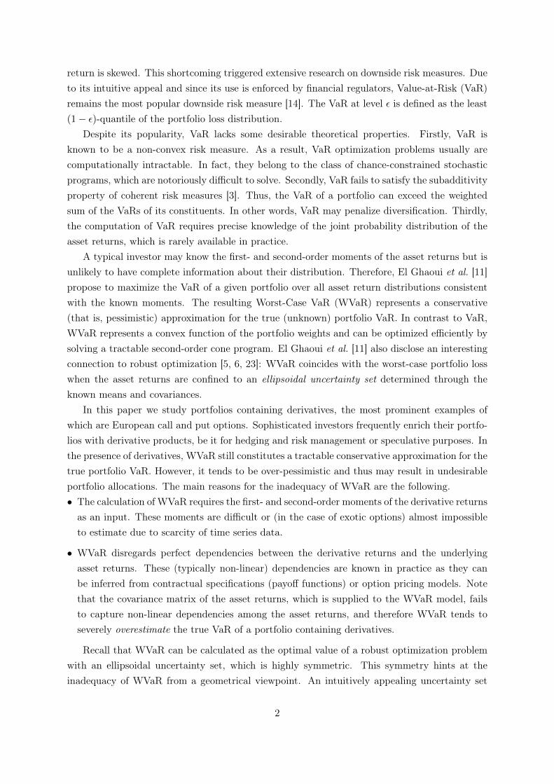
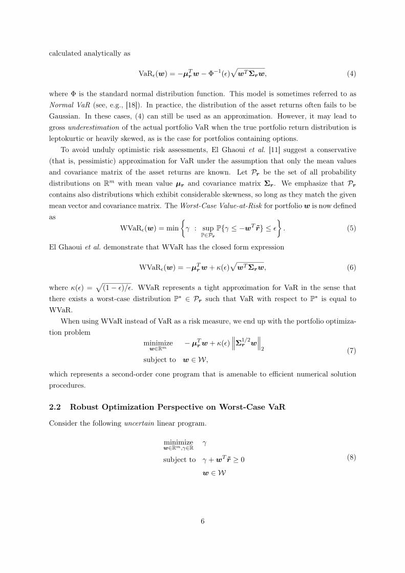
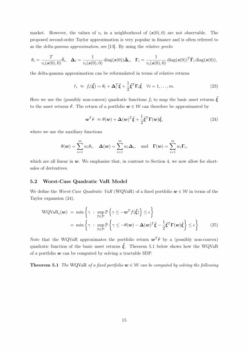
Figure 1: Left: The portfolio loss distribution obtained via Monte-Carlo simulation. Note that negative values representgains. Right: The VaR estimates at different confidence levels obtained via Monte-Carlo sampling, WVaR, and WPVaR.
Example 4.1 Consider a Black-Scholes economy consisting of stocks A and B, a European calloption on stock A, and a European put option on stock B. Furthermore, let w be an equallyweighted portfolio of these m = 4 assets, that is, set wi = 1/m for i = 1, . . . ,m. We assumethat the prices of stocks A and B are governed by a bivariate geometric Brownian motion withdrift coefficients of 12% and 8%, and volatilities of 30% and 20% per annum, respectively. Thecorrelation between the instantaneous stock returns amounts to 20%. The initial prices of thestocks are $100. The options mature in 21 days and have strike prices of $100. We assume thatthe risk-free rate is 3% per annum and that there are 252 trading days per year. By using theBlack-Scholes formulas [8], we obtain call and put option prices of $3.58 and $2.18, respectively.
We want to compute the VaR at confidence level ε for portfolio w and a 21-day time horizon.To this end, we randomly generate L=5,000,000 end-of-period stock prices and correspondingoption payoffs. These are used to obtain L asset and portfolio return samples. Figure 1 (left)displays the sampled portfolio loss distribution, which exhibits considerable skewness due to theoptions. The Monte-Carlo VaR is obtained by computing the (1 − ε)-quantile of the sampledportfolio loss distribution. We also compute the sample means and sample covariance matrix ofthe asset returns, which are used for the calculation of WVaR (6) and WPVaR (18).
Figure 1 (right) displays the VaR estimates at different levels of ε ∈ [0.01, 0.2]. We observethat for all values of ε, the WVaR and WPVaR values exceed the Monte-Carlo VaR estimate.This is not surprising since these models are distributionally robust and as such provide a conser-vative estimate of VaR. Note that the Monte-Carlo VaR can only be calculated accurately if manyreturn samples are available (e.g., if the return distribution is precisely known). However, WVaR
vastly overestimates WPVaR. This effect is amplified for lower values of ε, where the accuracyof the VaR estimate matters most. Indeed, for ε = 1%, the WVaR reports an unrealistically highvalue of 497%, which is 7 times larger than the corresponding WPVaR value.
13
5 Worst-Case Quadratic VaR Optimization
The WPVaR model suffers from a number of weaknesses which may make it unattractive forcertain investors. Firstly, in order to obtain a tractable problem reformulation we had to prohibitshort-sales of options. Although this is not restrictive for investors who merely want to enrichtheir portfolios with options in order to obtain insurance benefits (see [29]), it severely constrainsthe complete set of option strategies that larger institutions might want to include in theirportfolios. Furthermore, we can only calculate and optimize the risk of portfolios comprisingoptions that mature at the end of the investment horizon. As a result, investors cannot use themodel, for example, to optimize portfolios including longer term options that mature far beyondthe investment horizon. Finally, the model is only suitable for portfolios containing plain vanillaEuropean options and can not be used when exotic options are included in the portfolio.
In this section we propose an alternative Worst-Case VaR model which mitigates the weak-nesses of the WPVaR model. It is important to note that WPVaR does not make any assump-tions about the pricing model of the options. Only observable market prices and the knownpayoff functions of the options are used to calculate the option returns. In contrast, the newmodel proposed in this section requires the availability of a pricing model for the options. More-over, it approximates the portfolio return using a second-order Taylor expansion which is onlyaccurate for short investment horizons.
5.1 Delta-Gamma Portfolio Model
As in Section 4, we assume that there are n ≤ m basic assets and m−n derivatives whose valuesare uniquely determined by the values of the basic assets. However, in contrast to Section 4, wedo not only focus on European style options but also allow for exotic derivatives. Furthermore,we no longer require that the options mature at the end of the investment horizon.
We let s(t) denote the n-dimensional vector of basic asset prices at time t ≥ 0 and assumethat the prices at time t = 0 are known (i.e., deterministic). Moreover, we assume that the valueof any (basic or non-basic) asset i = 1, . . . ,m is representable as vi(s(t), t), where vi : Rn×R→ Ris twice continuously differentiable.
For a sufficiently short horizon time T , a second-order Taylor expansion accurately approxi-mates the asset values at the end of the investment horizon. For i = 1, . . . ,m we have
vi(s(T ), T )− vi(s(0), 0) ≈ θiT + ∆Ti (s(T )− s(0)) +
1
2(s(T )− s(0))T Γi(s(T )− s(0)),
where
θi = ∂tvi(s(0), 0) ∈ R, ∆i = ∇svi(s(0), 0) ∈ Rn, and Γi = ∇2svi(s(0), 0) ∈ Sn. (22)
The values computed in (22) are referred to as the ‘greeks’ of the assets. We emphasize that thecomputation of the greeks relies on the availability of a pricing model, that is, the value functionsvi must be known. Note that the values of the functions vi at (s(0), 0) can be observed in the
14
market. However, the values of vi in a neighborhood of (s(0), 0) are not observable. Theproposed second-order Taylor approximation is very popular in finance and is often referred toas the delta-gamma approximation, see [13]. By using the relative greeks
θi =T
vi(s(0), 0)θi, ∆i =
1
vi(s(0), 0)diag(s(0))∆i, Γi =
1
vi(s(0), 0)diag(s(0))T Γi diag(s(0)),
the delta-gamma approximation can be reformulated in terms of relative returns
ri ≈ fi(ξ) = θi + ∆Ti ξ +
1
2ξTΓiξ ∀i = 1, . . . ,m. (23)
Here we use the (possibly non-convex) quadratic functions fi to map the basic asset returns ξto the asset returns r. The return of a portfolio w ∈ W can therefore be approximated by
wT r ≈ θ(w) + ∆(w)T ξ +1
2ξTΓ(w)ξ, (24)
where we use the auxiliary functions
θ(w) =
m∑i=1
wiθi, ∆(w) =
m∑i=1
wi∆i, and Γ(w) =
m∑i=1
wiΓi,
which are all linear in w. We emphasize that, in contrast to Section 4, we now allow for short-sales of derivatives.
5.2 Worst-Case Quadratic VaR Model
We define the Worst-Case Quadratic VaR (WQVaR) of a fixed portfolio w ∈ W in terms of theTaylor expansion (24).
WQVaRε(w) = min
γ : sup
P∈PPγ ≤ −wT f(ξ)
≤ ε
= min
γ : sup
P∈PPγ ≤ −θ(w)−∆(w)T ξ − 1
2ξTΓ(w)ξ
≤ ε
(25)
Note that the WQVaR approximates the portfolio return wT r by a (possibly non-convex)quadratic function of the basic asset returns ξ. Theorem 5.1 below shows how the WQVaRof a portfolio w can be computed by solving a tractable SDP.
Theorem 5.1 The WQVaR of a fixed portfolio w ∈ W can be computed by solving the following
15
tractable SDP
WQVaRε(w) = inf γ
s. t. M ∈ Sn+1, τ ∈ R, γ ∈ R
〈Ω,M〉 ≤ τε, M < 0, τ ≥ 0,
M +
[Γ(w) ∆(w)
∆(w)T −τ + 2(γ + θ(w))
]< 0,
(26)
where Ω is the second-order moment matrix of ξ; see (17).
Proof: See Appendix B.
Remark 5.1 The WQVaR model described here assumes the underlying asset returns to be theonly sources of uncertainty in the market. It is known, however, that implied volatilities constituteimportant risk factors for portfolios containing options. In particular, long dated options arehighly sensitive to fluctuations in the volatilities of the underlying assets. The sensitivity of theportfolio return with respect to the volatilities is commonly referred to as vega risk. The WQVaR
model can easily be modified to include implied volatilities as additional risk factors. The arisingdelta-gamma-vega-approximation of the portfolio return is still a quadratic function of the riskfactors. Thus, all derivations presented here remain valid in this generalized setting.
As in the case of WPVaR, it is possible to extend the WQVaR model to account for parti-tioned statistics information and for box-type uncertainty in the moment matrix Ω by extendingtechniques proposed in [20] in a straightforward manner; see also Remarks 4.3 and 4.4.
Remark 5.2 If the market only contains basic assets and no derivatives, then m = n, and thecoefficient functions in the delta-gamma approximation (24) reduce to θ(w) = 0, ∆(w) = w,and Γ(w) = 0. In this special case, the WQVaR is computed by solving the following SDP.
WQVaRε(w) = inf γ
s. t. M ∈ Sn+1, τ ∈ R, γ ∈ R
〈Ω,M〉 ≤ τε, M < 0, τ ≥ 0
M +
[0 w
wT −τ + 2γ
]< 0
El Ghaoui et al. [11] have shown (using similar arguments as in Theorem 4.2) that this SDPhas the closed form solution
WVaRε(w) = −µTw + κ(ε)√wTΣw, where κ(ε) =
√1− εε
.
Thus, the WQVaR model is a direct extension of the WVaR model (6).
16
Problem (26) constitutes a convex SDP that facilitates the efficient computation of theWQVaR for any fixed portfolio w ∈ W. Since the matrix inequality in (26) is linear in (M, τ , γ)
and w, one can reinterpret w as a decision variable without impairing the problem’s convexity.This observation reveals that we can efficiently minimize the WQVaR over all portfolios w ∈ Wby solving the following SDP.
inf γ
s. t. M ∈ Sn+1, τ ∈ R, γ ∈ R, w ∈ W
〈Ω,M〉 ≤ τε, M < 0, τ ≥ 0
M +
[Γ(w) ∆(w)
∆(w)T −τ + 2(γ + θ(w))
]< 0
(27)
Remark 5.3 Unlike in Section 4, there seems to be no equivalent SOCP formulation for the SDP(27). In particular, there is no simple way to adapt the arguments in the proof of Theorem 4.2to the current setting. The reason for this is a fundamental difference between the correspondingSDP problems (16) and (27). In fact, the top left principal submatrix in the last LMI constraintis independent of w in (16) but not in (27).
5.3 Robust Optimization Perspective on WQVaR
We now highlight the close connection between robust optimization and WQVaR minimization.In the next theorem we elaborate an equivalence between the WQVaR minimization problemand a robust optimization problem whose uncertainty set is embedded into a space of positivesemidefinite matrices.
Theorem 5.2 The WQVaR minimization problem (27) is equivalent to the robust optimizationproblem
minimizew∈Rm,γ∈R
γ
subject to − 〈Q(w),Z〉 ≤ γ ∀Z ∈ Uqεw ∈ W,
(28)
where
Q(w) =
[12Γ(w) 1
2∆(w)12∆(w)T θ(w)
],
and the uncertainty set Uqε ⊆ Sn+1 is defined as
Uqε =
Z =
[X ξ
ξT 1
]∈ Sn+1 : Ω− εZ < 0, Z < 0
. (29)
Proof: See Appendix B.
17

It may not be evident how the uncertainty set Uqε (defined in (29)) associated with the WQVaR
formulation is related to the ellipsoidal uncertainty set Uε defined in Section 2.2. We nowdemonstrate that there exists a strong connection between these two uncertainty sets, eventhough they are embedded in spaces of different dimensions.
Corollary 5.1 If the constraint Γ(w) < 0 is appended to the definition of the set W of admis-sible portfolios, then the robust optimization problem (28) reduces to
minimizew∈Rm,γ∈R
γ
subject to − θ(w)−∆(w)T ξ − 1
2ξTΓ(w)ξ ≤ γ ∀ξ ∈ Uε
w ∈ W,
(30)
where Uε is the ellipsoidal uncertainty set defined in Section 2.2.
Proof: See Appendix B.
Remark 5.4 Note that the robust optimization problem (30) can be reformulated as
minimizew∈Rm,γ∈R
γ
subject to −wTr ≤ γ ∀r ∈ Uq2εw ∈ W,
(31)
where the uncertainty set Uq2ε is defined as
Uq2ε =
r ∈ Rm :
∃ξ ∈ Rn such that(ξ − µ)TΣ−1(ξ − µ) ≤ κ(ε)2 andri = θi + ξT∆i + 1
2ξTΓiξ ∀i = 1, . . . ,m
In contrast to the simple ellipsoidal set Uε, the set Uq2ε is asymmetrically oriented around µ. Thisasymmetry is caused by the quadratic functions that map the basic asset returns ξ to the assetreturns r. As a result, the WQVaR model may provide a tighter approximation of the actualVaR of a portfolio containing derivatives than the WVaR model.
It seems that a min-max formulation (31) with an uncertainty set embedded into Rm is onlyavailable if Γ(w) < 0, that is, if the portfolio return is a convex quadratic function of the basicassets returns. In general, however, one needs to resort to the more general formulation (28),in which the uncertainty set is embedded into Sn+1; the dimension increase can compensate forthe non-convexity of the portfolio return function.
Example 5.1 We repeat the same experiment as in Example 4.1 but estimate the portfolio VaRafter 2 days instead of 21 days. Since the VaR is no longer evaluated at the maturity time of the
18
0
1
2
3
4
5
6
7
-1 -0.8 -0.6 -0.4 -0.2 0 0.2 0.4 0.6
pro
babili
ty (
%)
portfolio loss
0
0.2
0.4
0.6
0.8
1
1.2
1.4
80 82 84 86 88 90 92 94 96 98 100
VaR
Confidence level (1-ε)%
Monte-Carlo VaRWorst-Case VaR
Worst-Case Quadratic VaR
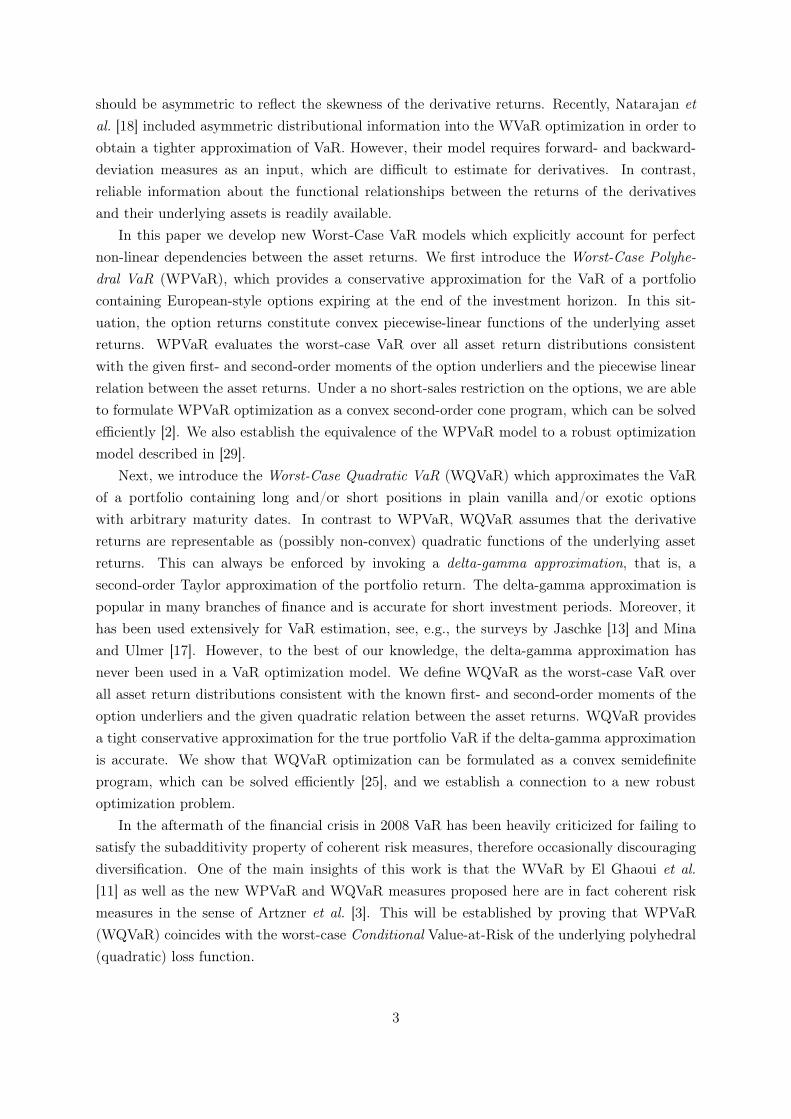
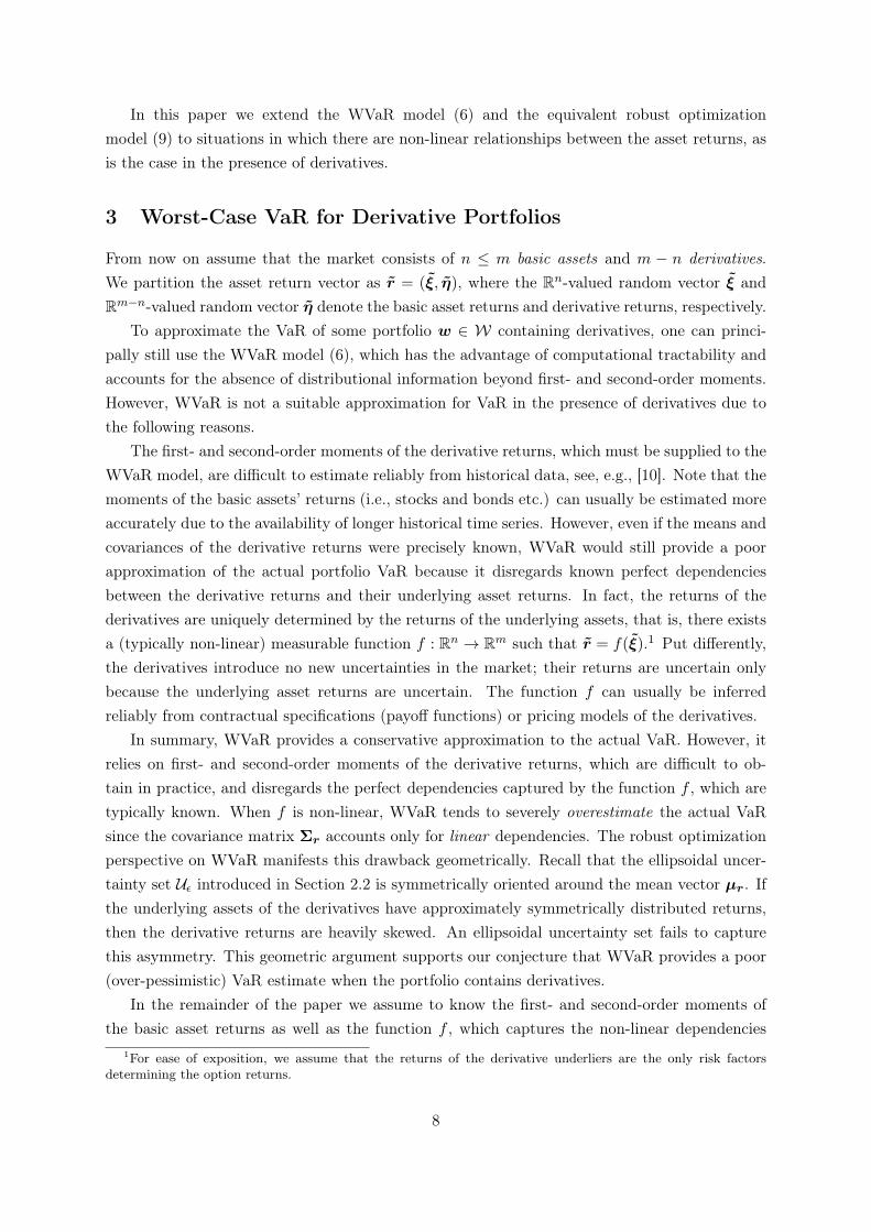
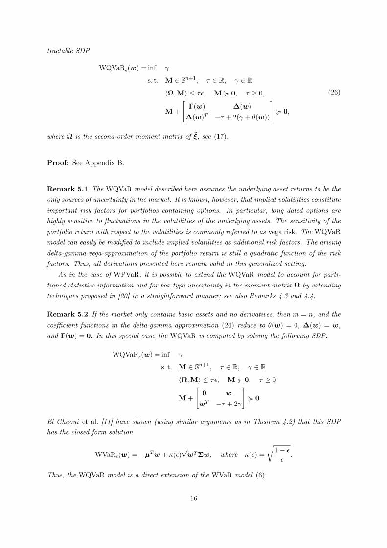
Figure 2: Left: The portfolio loss distribution obtained via Monte-Carlo simulation. Note that negative values representgains. Right: The VaR estimates at different confidence levels obtained via Monte-Carlo sampling, WVaR, and WQVaR.
options, we use the WQVaR model instead of the WPVaR model. The coefficients of the quadraticapproximation function (24) are calculated using the standard Black-Scholes greek formulas (see,e.g., [15]). We use an analogous Monte-Carlo simulation as in Example 4.1 to generate the stockand option returns over a 2-day investment period as well as the corresponding sample means andcovariances. Figure 2 (left) displays the sampled portfolio loss distribution, which is still skewed,although considerably less than in Example 4.1. In Figure 2 (right) we compare Monte-CarloVaR, WVaR, and WQVaR for different confidence levels. Even for the short horizon time underconsideration, the WVaR model still fails to give a realistic VaR estimate. At ε = 1%, WVaR ismore than 3 times as large as the corresponding WQVaR value. This example demonstrates thatWQVaR can offer significantly better VaR estimates than WVaR when the portfolio containsoptions.
6 Relation to Worst-Case Conditional Value-at-Risk
We now establish a connection between the VaR-based risk measures proposed in Sections 4and 5 and two Conditional Value-at-Risk (CVaR) measures, which are coherent in the sense ofArtzner et al. [3]. This equivalence will then allow us to conclude that WPVaR and WQVaR arecoherent risk measures over spaces of restricted portfolio returns. Coherence of risk measuresfrom a robust optimization perspective has also been investigated by Natarajan et al. [19].
The classical CVaR is a quantile-based risk measure which evaluates the conditional expec-tation of the portfolio loss above VaR. For a given probability distribution P of r and toleranceε ∈ (0, 1), Rockafellar and Uryasev [22] define the CVaR of a portfolio w ∈ Rm as
CVaRε(w) = infβ∈R
β +
1
εEP((−wT r − β)+
),
where EP(·) denotes expectation with respect to P. By construction, CVaR is convex in w and—unlike VaR—constitutes a coherent risk measure [1]. If only the mean vector µr and covariancematrix Σr 0 of r are known, CVaR does not admit exact evaluation. As in the case of VaR,
19

it then proves useful to introduce the Worst-Case CVaR (WCVaR)
WCVaRε(w) = supP∈Pr
infβ∈R
β +
1
εEP(−wT r − β)+
,
where Pr denotes the set of probability distributions of r consistent with the given mean vectorµr and covariance matrix Σr.
If a portfolio includes long positions in derivatives expiring at the end of the investmenthorizon as in Section 4, WCVaR may be an overly conservative risk measure. In analogy toWPVaR we thus introduce the Worst-Case Polyhedral CVaR (WPCVaR),
WPCVaRε(w) = supP∈P
infβ∈R
β +
1
εEP
(−(wξ)T ξ − (wη)T max−e,a+ Bξ − e − β
)+,
which faithfully accounts for the known dependencies among the derivatives and their underlyingassets. Here, P denotes the usual set of all distributions of the derivative underliers which sharethe same mean vector µ and covariance matrix Σ. Similarly, for portfolios including derivativesthat expire far beyond the investment horizon as in Section 5, we can define the Worst-CaseQuadratic CVaR (WQCVaR) as follows.
WQCVaRε(w) = supP∈P
infβ∈R
β +
1
εEP
(−θ(w)−∆(w)T ξ − 1
2ξTΓ(w)ξ − β
)+
The next theorem establishes a connection between these new CVaR-based risk measures andthe WPVaR and WQVaR measures introduced in Sections 4 and 5, respectively.
Theorem 6.1 The following identities hold:
(i) WPVaRε(w) = WPCVaRε(w) for all w = (wξ,wη) ∈ Rn × Rm−n+ ;
(ii) WQVaRε(w) = WQCVaRε(w) for all w ∈ Rm.
Proof: The claim is an immediate consequence of an exactness result about Worst-Case CVaRapproximations for distributionally robust chance constraints with convex or (possibly non-convex) quadratic constraint functions [28, Theorem 2.2].
Corollary 6.1 WPVaR is a coherent risk measure on the cone of polyhedral portfolio returns
RP =rp = (wξ)T ξ + (wη)T max−e,a+ Bξ − e : wξ ∈ Rn, wη ∈ Rm−n+
.
Similarly, WQVaR is a coherent risk measure on the subspace of quadratic portfolio returns
RQ =
rp = θ(w) + ∆(w)T ξ +
1
2ξTΓ(w)ξ : w ∈ Rm
.
Proof: The known coherence of the classical CVaR for any given distribution P, see e.g. [1],implies via [27, Proposition 1] that WPCVaR is coherent on RP. By the equivalence of WPVaR
20

and WPCVaR established in Theorem 6.1, WPVaR is thus a coherent risk measure on RP.Coherence of WQVaR on RQ is proved in a similar manner.
Recall that the classical WVaR by El Ghaoui et al. [11] represents a special case of WPVaR (orWQVaR). Thus, an important consequence of Corollary 6.1 is that WVaR is a coherent riskmeasure on the space of all portfolio returns of the form wT r for w ∈ Rm.
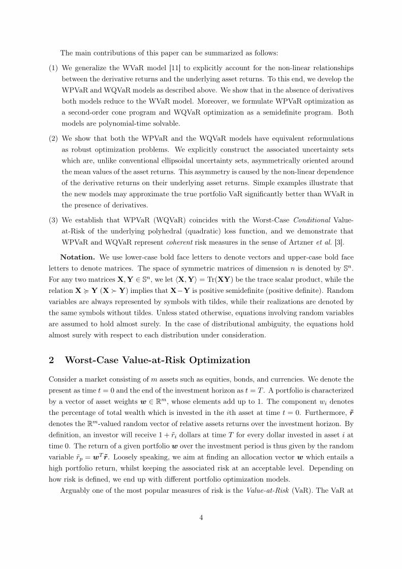
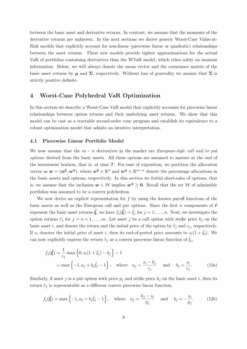
Example 6.1 (Index Tracking) We compare the out-of-sample performance of VaR, CVaR,WVaR and WQVaR in an index tracking experiment with real data taken from the OptionmetricsIvyDB database. The aim is to replicate the S&P 500 (SPX) index with a portfolio consisting ofthe NASDAQ-100 (NDX) and Russell 2000 (RUT) indices as well as two at-the-money Europeancall options on NASDAQ-100 and Russell 2000, respectively. The experiment covers 265 biweeklyrebalancing intervals from February 6 2001 to March 30 2011. In each rebalancing interval andfor both underliers we select the option with minimum bid-ask spread among all available optionsexpiring within the next two to three months. This choice of maturity dates ensures that theoption returns admit a delta-gamma approximation. The high liquidity of the index optionsallows us to assume that they can be purchased or sold anytime during the backtest period. Thehistorical bid-ask spreads average at 3.8% and 3.2% for the chosen options on NASDAQ-100 andRussell 2000, respectively. In order to ensure a fair reflection of liquidity risk, we artificiallyinflate the bid-ask spreads of the options to 5%. The bid-ask spreads of the option underliers areassumed to vanish, while the confidence level of the risk measures is set to ε = 5%.
At the start of each rebalancing interval we minimize the risk of the tracking portfolio’sexcess return over the benchmark. We use a rolling estimation window of three years (178data points) to calibrate the arising optimization models. VaR and CVaR are evaluated underthe empirical (discrete) distribution implied by the return observations in the estimation window.Thus, the underlying optimization problems can be reformulated as mixed-integer linear programsand linear programs, respectively, see e.g. [12, 22]. Similarly, WVaR and WQVaR are evaluatedusing the sample means and covariances implied by the data in the rolling estimation window.The underlying optimization models can be reformulated as SOCPs and SDPs, respectively, seeSection 2.1 and Theorem 5.1. The WQVaR model additionally requires information about theoptions’ delta, gamma and theta sensitivities. These are obtained from the implied volatilitiesreported in the Optionmetrics database and are calculated using the Black-Scholes formula.
On average, the arising linear and mixed-integer linear programs are solved in 16ms and206ms using ILOG CPLEX, while the SOCPs and SDPs are solved in 91ms and 195ms withSDPT3 [24], respectively. In general, the optimal CVaR, WVaR and WQVaR-portfolios canbe computed in time polynomial in the number of stocks and options via efficient interior pointalgorithms [26]. For example, we have found that instances of the WQVaR optimization modelinvolving 180 stocks and 180 options can conveniently be solved in less than one hour. In contrast,the VaR optimization problems involve binary variables and permit no polynomial time solution.Figure 3 visualizes the cumulative returns of the four tracking portfolios relative to the cumulativereturn of S&P 500. In this example the WQVaR-portfolio exceeds the benchmark over 80.4% ofthe time. In contrast, the WVaR-portfolio exceeds the benchmark only 7.8% of the time, while
21

2001 2003 2005 2007 2009 2012 0.7
0.8
0.9
1
1.1
1.2
1.3
1.4
Time
Tota
l R
etu
rn r
ela
tive to S
&P
500
VaR
CVaR
WVaR
WQVaR
Figure 3: Out-of-sample performance of different tracking portfolios
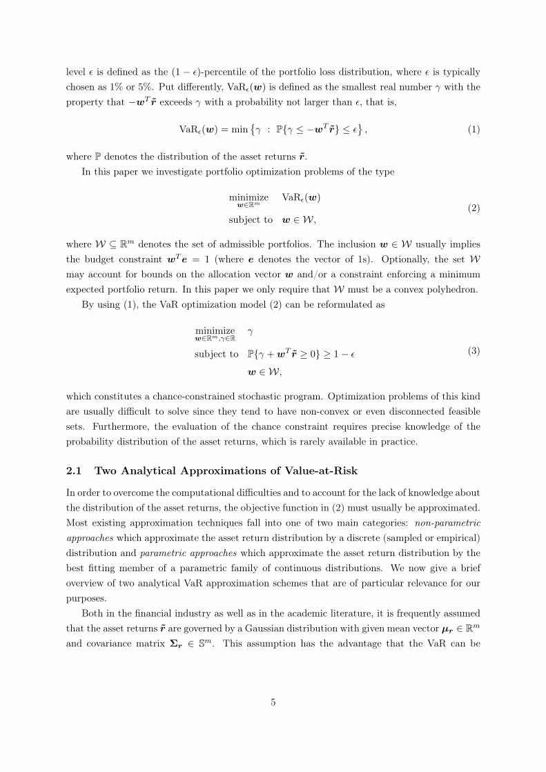
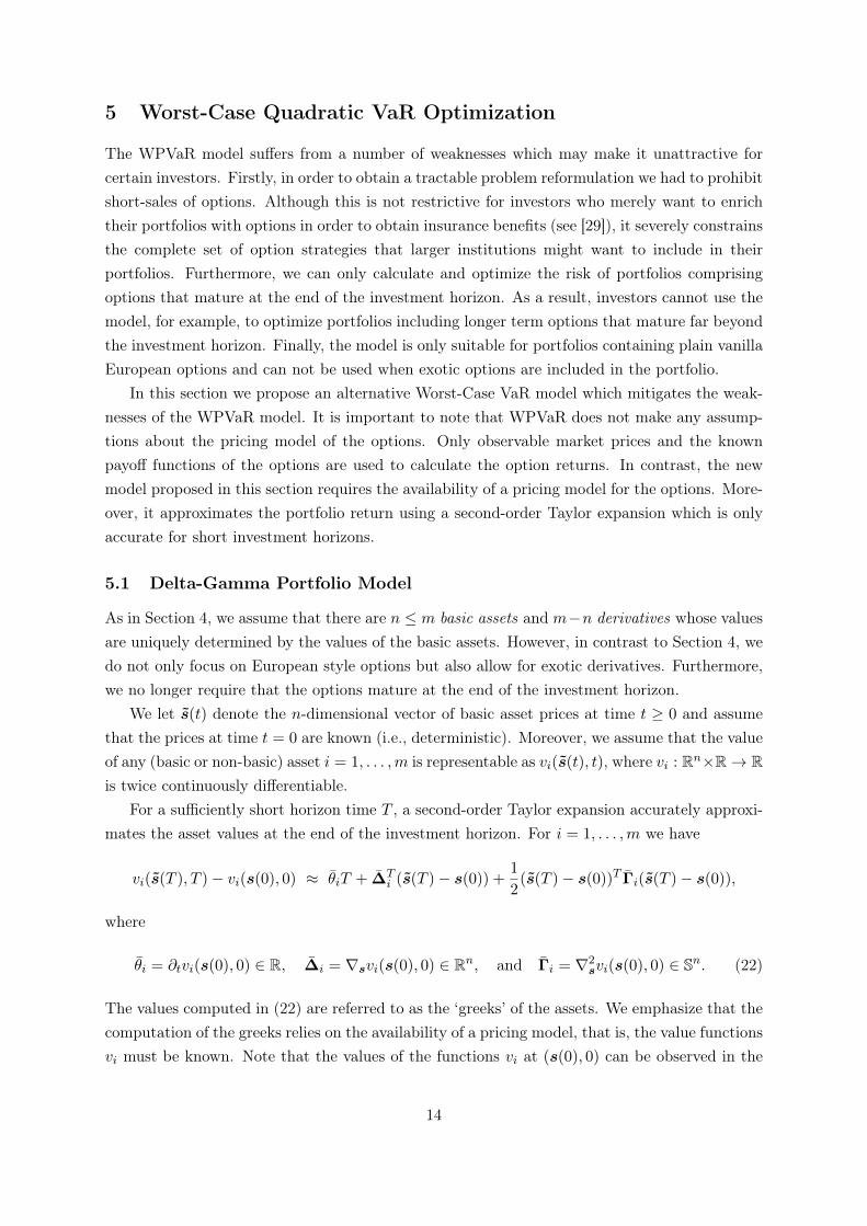
Table 1: Left: Out-of-sample statistics of excess return over the benchmark for different tracking portfolios (in basispoints). Right: Quadratic variation of the hedging instruments’ portfolio weights in the different tracking portfolios.
Statistic VaR CVaR WVaR WQVaR
Mean 1.3 -10.5 -4.1 10.0Std Dev 183.5 150.6 143.8 145.4VaR 313.8 236.3 240.2 208.6CVaR 412.0 365.2 342.7 311.3
Instrument VaR CVaR WVaR WQVaR
NDX 72.733 7.252 4.711 3.730RUT 68.073 7.326 4.864 3.738Call on NDX 0.586 0.108 0.062 0.069Call on RUT 0.257 0.121 0.090 0.080
the portfolios based on CVaR and VaR fall consistently short of the benchmark. Table 1 reportsout-of-sample statistics of the portfolios’ excess returns over S&P 500. We observe that theexcess return of the WQVaR-portfolio has the highest out-of-sample mean and the lowest out-of-sample VaR and CVaR (consistently computed at ε = 5%) among all tracking portfolios. Weremark that any discrepancies in the performance of the WVaR and WQVaR-portfolios can onlyoriginate from the different treatment of the options in these models. The non-robust trackingportfolios based on VaR and CVaR tend to be overfitted to the empirical return distributions andare therefore prone to error maximisation phenomena. Moreover, the corresponding portfolioweights are less stable than those of the WVaR and WQVaR-portfolios. Table 1 reports thequadratic variations, that is, the summed squared differences of all successive portfolio weightsthroughout the backtest period. The quadratic variation of a stochastic process can be regardedas a measure of its smoothness. We observe that the quadratic variations corresponding to theportfolio weights in the WQVaR-portfolio are almost two orders of magnitude smaller than thoseof the VaR-portfolio, and they are also significantly smaller than those of the CVaR and WVaR-portfolios. We therefore conclude that the WQVaR-portfolio is least affected by data noise.
7 Conclusions
Derivatives depend non-linearly on their underlying assets. In this paper we explicitly incorpo-rate this non-linear relationship into the WVaR model, which results in two new models. The
22

WPVaR model expresses the option returns as convex-piecewise linear functions of the under-lying assets and is therefore suited for portfolios containing European options maturing at theinvestment horizon. A benefit of this model is that it does not require knowledge of the pricingmodels of the options in the portfolio. However, in order to be tractably solvable, the WPVaR
model precludes short-sales of options. The WQVaR model, on the other hand, can handle port-folios containing non-European options and does not rely on short-sales restrictions. It exploitsthe popular delta-gamma approximation to model the portfolio return. In contrast to WPVaR,however, WQVaR does require knowledge of suitable option pricing models to determine thedelta-gamma approximation. Through numerical experiments we demonstrate that the WPVaR
and WQVaR models can provide much tighter VaR estimates of an options portfolio than theWVaR model, which disregard any non-linear dependencies between the asset returns. We alsodemonstrate that WQVaR, WPVaR and WVaR are equivalent to the corresponding worst-caseCVaR risk measures, which implies that they are actually coherent—in marked contrast to theclassical non-robust VaR.
Acknowledgments. We are indebted to Prof. A. Ben-Tal for valuable discussions on the topicsof this paper and to Grani Hanasusanto for his assistance with the numerical experiments. Thisresearch has been supported by EPSRC under grant EP/I014640/1.
References
[1] C. Acerbi and D. Tasche. On the coherence of expected shortfall. Journal of Banking &Finance, 26(7):1487–1503, 2002.
[2] F. Alizadeh and D. Goldfarb. Second-order cone programming. Mathematical Programming,95(1):3–51, 2003.
[3] P. Artzner, F. Delbaen, J. Eber, and D. Heath. Coherent measures of risk. MathematicalFinance, 9(3):203–228, 1999.
[4] A. Ben-Tal, L. El Ghaoui, and A. Nemirovski. Robust Optimization. Princeton UniversityPress, 2009.
[5] A. Ben-Tal and A. Nemirovski. Robust convex optimization. Mathematics of OperationsResearch, 23(4):769–805, 1998.
[6] A. Ben-Tal and A. Nemirovski. Robust solutions of uncertain linear programs. OperationsResearch Letters, 25(1):1–13, 1999.
[7] D. Bertsimas and M. Sim. The price of robustness. Operations Research, 52(1):35–53, 2004.
[8] F. Black and M. Scholes. The pricing of options and corporate liabilities. Journal of PoliticalEconomy, 81(3):637–54, 1973.
23

[9] G. Calafiore, U. Topcu, and L. El Ghaoui. Parameter estimation with expected and residual-at-risk criteria. Systems & Control Letters, 58(1):39–46, 2009.
[10] J. Coval and T. Shumway. Expected option returns. The Journal of Finance, 56(3):983 –1009, 2002.
[11] L. El Ghaoui, M. Oks, and F. Oustry. Worst-case value-at-risk and robust portfolio opti-mization: A conic programming approach. Operations Research, 51(4):543–556, 2003.
[12] A. Gaivoronski and G. Pflug. Value-at-Risk in portfolio optimization: Properties andcomputational approach. Journal of Risk, 7(2):1–31, 2005.
[13] S. Jaschke. The cornish-fisher expansion in the context of delta-gamma-normal approxima-tions. Journal of Risk, 4(4):33–53, 2002.
[14] P. Jorion. Value-at-Risk: The New Benchmark for Managing Financial Risk. McGraw-Hill,2001.
[15] L. MacMillan. Options as a strategic investment. Prentice Hall, 1992.
[16] H. Markowitz. Portfolio selection. Journal of Finance, 7(1):77–91, 1952.
[17] J. Mina and A. Ulmer. Delta-gamma four ways. Technical report, RiskMetrics Group, 1999.
[18] K. Natarajan, D. Pachamanova, and M. Sim. Incorporating asymmetric distributionalinformation in robust value-at-risk optimization. Management Science, 54(3):573–585, 2008.
[19] K. Natarajan, D. Pachamanova, and M. Sim. Constructing risk measures from uncertaintysets. Operations Research, 57(5):1129–1141, 2009.
[20] K. Natarajan, M. Sim, and J. Uichanco. Tractable robust expected utility and risk modelsfor portfolio optimisation. Mathematical Finance, 20(4):695–731, 2010.
[21] I. Pólik and T. Terlaky. A survey of the S-lemma. SIAM Review, 49(3):371–481, 2007.
[22] R. Rockafellar and S. Uryasev. Optimization of conditional value-at-risk. Journal of Risk,2:21–41, 2002.
[23] B. Rustem and M. Howe. Algorithms for Worst-Case Design and Applications to RiskManagement. Princeton University Press, 2002.
[24] R. H. Tütüncü, K. C. Toh, and M. J. Todd. Solving semidefinite-quadratic-linear programsusing SDPT3. Mathematical Programming Ser. B, 95:189–217, 2003.
[25] L. Vandenberghe and S. Boyd. Semidefinite programming. SIAM Review, 38(1):49–95,1996.
[26] Yinyu Ye. Interior point algorithms: theory and analysis. John Wiley & Sons, Inc., NewYork, NY, USA, 1997.
24
[27] S. Zhu and M. Fukushima. Worst-case conditional value-at-risk with application to robustportfolio management. Operations Research, 57(5):1155–1168, 2009.
[28] S. Zymler, D. Kuhn, and B. Rustem. Distributionally robust joint chance constraints withsecond-order moment information. Mathematical Programming, 2011. Forthcoming.
[29] S. Zymler, B. Rustem, and D. Kuhn. Robust portfolio optimization with derivative insur-ance guarantees. European Journal of Operational Research, 210(2):410–424, 2011.
A Worst-Case Probability Problems
In this appendix we review a general result about worst-case probability problems that plays akey role for many of the derivations in this paper.
Lemma A.1 (Calafiore et al. [9]) Let S ⊆ Rn be any Borel measurable set (which is notnecessarily convex), and define the worst-case probability πwc as
πwc = supP∈P
Pξ ∈ S, (32)
where P is the set of all probability distributions of ξ with mean vector µ and covariance matrixΣ 0. Then,
πwc = infM∈Sn+1
〈Ω,M〉 : M < 0,
[ξT 1
]M[ξT 1
]T ≥ 1 ∀ξ ∈ S,
where Ω is the second-order moment matrix of ξ; see (17).
B Proofs
Proof of Theorem 4.1 In order to derive a manifestly tractable representation for WPVaR,we first simplify the maximization problem
supP∈P
Pγ ≤ −(wξ)T ξ − (wη)T max
−e,a+ Bξ − e
, (33)
which can be identified as the subordinate optimization problem in (15).For some fixed portfolio w ∈ W and γ ∈ R, we define the set Sγ ⊆ Rn as
Sγ = ξ ∈ Rn : γ + (wξ)T ξ + (wη)T max−e,a+ Bξ − e ≤ 0.
For any ξ ∈ Rn and nonnegative wη ∈ Rm−n we have
(wη)T max−e,a+ Bξ − e = ming∈Rm−n
gTwη : g ≥ −e, g ≥ a+ Bξ − e
= maxy∈Rm−n
yT (a+ Bξ)− eTwη : 0 ≤ y ≤ wη
,
25

where the second equality follows from strong linear programming duality. Thus, the set Sγ canbe written as
Sγ =
ξ ∈ Rn : max
0≤y≤wη
γ + (wξ)T ξ + yT (a+ Bξ)− eTwη
≤ 0
. (34)
The optimal value of problem (33) is obtained by solving the worst-case probability problemsupP∈P
Pξ ∈ Sγ, which, by Lemma A.1 can be expressed as
infM∈Sn+1
〈Ω,M〉
s. t.[ξT 1
]M[ξT 1
]T ≥ 1 ∀ξ : max0≤y≤wη
γ + (wξ)T ξ + yT (a+ Bξ)− eTwη ≤ 0
M < 0.
(35)
We will now argue that (35) is equivalent to problem (36) below for all but one value of γ.
inf 〈Ω,M〉
s. t. M ∈ Sn+1, τ ∈ R, M < 0, τ ≥ 0[ξT 1
]M[ξT 1
]T− 1 + 2τ
(max
0≤y≤wηγ + (wξ)T ξ + yT (a+ Bξ)− eTwη
)≥ 0 ∀ξ ∈ Rn
(36)For ease of exposition, we first define
h = minξ∈Rn
max0≤y≤wη
γ + (wξ)T ξ + yT (a+ Bξ)− eTwη.
The equivalence of (35) and (36) is proved case by case. Assume first that h < 0. Then, theequivalence follows from the non-linear Farkas Lemma, see, e.g., [21, Theorem 2.1]. Assume nextthat h > 0. Then, the semi-infinite constraint in (35) becomes redundant and, since Ω 0,the optimal solution of (35) is given by M = 0 with a corresponding optimal value of 0. Theoptimal value of problem (36) is also equal to 0. Indeed, by choosing τ = 1/h, the semi-infiniteconstraint in (36) is satisfied independently of M. Finally, (35) and (36) may differ for h = 0.
It can be seen that since τ ≥ 0, the semi-infinite constraint in (36) is equivalent to theassertion that there exists some 0 ≤ y ≤ wη with
[ξT 1
]M[ξT 1
]T − 1 + 2τ(γ + (wξ)T ξ + yT (a+ Bξ)− eTwη
)≥ 0 ∀ξ ∈ Rn.
This semi-infinite constraint can be written as[ξ
1
]T (M +
[0 τ(wξ + BTy)
τ(wξ + BTy)T −1 + 2τ(γ + yTa− eTwη)
])[ξ
1
]≥ 0 ∀ξ ∈ Rn
⇐⇒ M +
[0 τ(wξ + BTy)
τ(wξ + BTy)T −1 + 2τ(γ + yTa− eTwη)
]< 0.
26
Thus, problem (36) can equivalently be formulated as
inf 〈Ω,M〉
s. t. M ∈ Sn+1, y ∈ Rm−n, τ ∈ R
M < 0, τ ≥ 0, 0 ≤ y ≤ wη
M +
[0 τ(wξ + BTy)
τ(wξ + BTy)T −1 + 2τ(γ + yTa− eTwη)
]< 0.
(37)
Since (35) and (37) are equivalent for all but one value of γ and since their optimal values arenonincreasing in γ, we can express WPVaR in (15) as the optimal value of the following problem.
WPVaRε(w) = inf γ
s. t. M ∈ Sn+1, y ∈ Rm−n, τ ∈ R, γ ∈ R
〈Ω,M〉 ≤ ε, M < 0, τ ≥ 0, 0 ≤ y ≤ wη
M +
[0 τ(wξ + BTy)
τ(wξ + BTy)T −1 + 2τ(γ + yTa− eTwη)
]< 0
(38)
Problem (38) is non-convex due to the bilinear terms in the matrix inequality constraint. It caneasily be shown that 〈Ω,M〉 ≥ 1 for any feasible point with vanishing τ -component. However,since ε < 1, this is in conflict with the constraint 〈Ω,M〉 ≤ ε. We thus conclude that no feasiblepoint can have a vanishing τ -component. This allows us to divide the matrix inequality inproblem (38) by τ . Subsequently we perform variable substitutions in which we replace τ by1/τ and M by M/τ . This shows that (38) is equivalent to problem (16).
Proof of Theorem 5.1 For the given portfolio w ∈ W and for any fixed γ ∈ R, we introducethe set Qγ ⊆ Rn, defined through
Qγ =
ξ ∈ Rn : γ ≤ −θ(w)−∆(w)T ξ − 1
2ξTΓ(w)ξ
. (39)
As in Section 4, the first step towards a tractable reformulation of WQVaR is to solve theworst-case probability problem
πwc = supP∈P
Pξ ∈ Qγ, (40)
which can be identified as the subordinate maximization problem in (25). Lemma A.1 impliesthat (40) can equivalently be formulated as
πwc = infM∈Sn+1
〈Γ,M〉 : M < 0,
[ξT 1
]M[ξT 1
]T ≥ 1 ∀ξ ∈ Qγ. (41)
By the definition of Q, the semi-infinite constraint in problem (41) is equivalent to
[ξT 1
](M− diag(0, 1))
[ξT 1
]T ≥ 0 ∀ξ :[ξT 1
] [ 12Γ(w) 1
2∆(w)12∆(w)T γ + θ(w)
] [ξT 1
]T ≤ 0.
27
By using the S-lemma [21] and by analogous reasoning as in Section 4.2, we can replace thesemi-infinite constraint in problem (41) by
∃τ ≥ 0 : M +
[τΓ(w) τ∆(w)
τ∆(w)T −1 + 2τ(γ + θ(w))
]< 0
without changing the optimal value of the problem. Thus, the worst-case probability problem(40) can be rewritten as
πwc = inf 〈Ω,M〉
s. t. M ∈ Sn+1, τ ∈ R, M < 0, τ ≥ 0
M +
[τΓ(w) τ∆(w)
τ∆(w)T −1 + 2τ(γ + θ(w))
]< 0.
(42)
The WQVaR of the portfolio w can therefore be obtained by solving the following non-convexoptimization problem.
WQVaRε(w) = inf γ
s. t. M ∈ Sn+1, τ ∈ R, γ ∈ R
〈Ω,M〉 ≤ ε, M < 0, τ ≥ 0
M +
[τΓ(w) τ∆(w)
τ∆(w)T −1 + 2τ(γ + θ(w))
]< 0
(43)
By analogous reasoning as in Section 4.2, it can be shown that any feasible solution of prob-lem (43) has a strictly positive τ -component. Thus we may divide the matrix inequality in (43)by τ . After the variable transformation τ → 1/τ and M → M/τ , we obtain the postulatedSDP (26).
Proof of Theorem 5.2 For some fixed portfolio w ∈ W, the WQVaR can be computed bysolving problem (26), which involves the LMI constraint
M +
[Γ(w) ∆(w)
∆(w)T −τ + 2(γ + θ(w))
]< 0. (44)
Without loss of generality, we can rewrite the matrix M as
M =
[V v
vT u
].
28
With this new notation, the LMI constraint (44) is representable as
[ξT 1]
[V + Γ(w) v + ∆(w)
(v + ∆(w))T u− τ + 2(γ + θ(w))
][ξT 1]T ≥ 0 ∀ξ ∈ Rn
⇐⇒ ξT (V + Γ(w))ξ + 2ξT (v + ∆(w)) + u− τ + 2(γ + θ(w)) ≥ 0 ∀ξ ∈ Rn
⇐⇒ γ ≥ −1
2ξT (V + Γ(w))ξ − ξT (v + ∆(w))− θ(w)− 1
2(u− τ) ∀ξ ∈ Rn
⇐⇒ γ ≥ supξ∈Rn
−1
2ξT (V + Γ(w))ξ − ξT (v + ∆(w))− θ(w)− 1
2(u− τ)
.
Thus, the WQVaR problem (26) can be rewritten as
inf supξ∈Rn
−1
2ξT (V + Γ(w))ξ − ξT (v + ∆(w))− θ(w)− 1
2(u− τ)
s. t. V ∈ Sn, v ∈ Rn, τ ∈ R, u ∈ R[V v
vT u
]< 0, τ ≥ 0, 〈V,Σ + µµT 〉+ 2vTµ+ u ≤ τε.
(45)
Note that if V + Γ(w) is not positive semidefinite, the inner maximization problem in (45)is unbounded. However, this implies that any V ∈ Sn is infeasible in the outer minimizationproblem unless V + Γ(w) < 0. Therefore, we can add the constraint V + Γ(w) < 0 tothe minimization problem in (45) without changing its feasible region. With this constraintappended, the min-max problem (45) becomes a saddlepoint problem because its objective isconcave in ξ for any fixed (V,v, u, τ) and convex in (V,v, u, τ) for any fixed ξ. Moreover, thefeasible sets of the outer and inner problems are convex and independent of each other. Thus,we may interchange the ‘inf’ and ‘sup’ operators to obtain the following equivalent problem.
maxξ∈Rn
min − 1
2ξT (V + Γ(w))ξ − ξT (v + ∆(w))− θ(w)− 1
2(u− τ)
s. t. V ∈ Sn, v ∈ Rn, τ ∈ R, u ∈ R[V v
vT u
]< 0, τ ≥ 0, 〈V,Σ + µµT 〉+ 2vTµ+ u ≤ τε.
(46)
We proceed by dualizing the inner minimization problem in (46). After a few elementary sim-plification steps, this dual problem reduces to
max − 1
2〈Γ(w), ξξT + Y〉 − ξT∆(w)− θ(w)
s. t. Y ∈ Sn, α ∈ R, Y < 0, 1 ≤ α ≤ 1
ε[α(Σ + µµT )− (ξξT + Y) αµ− ξ
(αµ− ξ)T α− 1
]< 0.
(47)
Note that strong duality holds because the inner problem in (46) is strictly feasible for any ε > 0,
29

see [25]. This allows us to replace the inner minimization problem in (46) by the maximizationproblem (47), which yields the following equivalent formulation for the WQVaR problem (26).
max − 1
2〈Γ(w), ξξT + Y〉 − ξT∆(w)− θ(w)
s. t. Y ∈ Sn, ξ ∈ Rn, α ∈ R, Y < 0, 1 ≤ α ≤ 1
ε[α(Σ + µµT )− (ξξT + Y) αµ− ξ
(αµ− ξ)T α− 1
]< 0
We now introduce a new decision variable X = ξξT + Y, which allows us to reformulate theabove problem as
max − 1
2〈Γ(w),X〉 − ξT∆(w)− θ(w)
s. t. X ∈ Sn, ξ ∈ Rn, α ∈ R, 1 ≤ α ≤ 1
ε[α(Σ + µµT )−X αµ− ξ
(αµ− ξ)T α− 1
]< 0, X− ξξT < 0.
By definition of Ω as the second-order moment matrix of the basic asset returns, see (17), thefirst LMI constraint in the above problem can be rewritten as
αΩ−
[X ξ
ξT 1
]< 0.
Furthermore, by using Schur complements, the following equivalence holds.
X− ξξT < 0 ⇐⇒
[X ξ
ξT 1
]< 0
Therefore, problem (47) can be reformulated as
max −
⟨[12Γ(w) 1
2∆(w)12∆(w)T θ(w)
],
[X ξ
ξT 1
]⟩s. t. X ∈ Sn, ξ ∈ Rn, α ∈ R, 1 ≤ α ≤ 1
ε
αΩ−
[X ξ
ξT 1
]< 0,
[X ξ
ξT 1
]< 0.
Since the objective function is independent of α and Ω 0, the optimal choice for α is 1/ε; infact, this choice of α generates the largest feasible set. We conclude that the WQVaR for a fixed
30
portfolio w can be computed by solving the following problem.
max −
⟨[12Γ(w) 1
2∆(w)12∆(w)T θ(w)
],
[X ξ
ξT 1
]⟩
s. t. X ∈ Sn, ξ ∈ Rn, Ω− ε
[X ξ
ξT 1
]< 0,
[X ξ
ξT 1
]< 0
The WQVaR minimization problem (27) can therefore be expressed as the min-max problem
minw∈W
maxZ∈Uqε
−〈Q(w),Z〉, (48)
which is manifestly equivalent to the postulated semi-infinite program (28).
Proof of Corollary 5.1 The inner maximization problem in (48) can be written as
max − θ(w)−∆(w)T ξ − 1
2〈Γ(w),X〉
s. t. X ∈ Sn, ξ ∈ Rn, X− ξξT < 0[(Σ + µµT )− εX µ− εξ
(µ− εξ)T 1− ε
]< 0.
By introducing the decision variable Y = X − ξξT as in the proof of Theorem 5.2, the aboveproblem can be reformulated as
max − θ(w)−∆(w)T ξ − 1
2ξTΓ(w)ξ − 1
2〈Γ(w),Y〉
s. t. Y ∈ Sn, ξ ∈ Rn, Y < 0[(Σ + µµT )− ε(Y + ξξT ) µ− εξ
(µ− εξ)T 1− ε
]< 0.
(49)
We will now argue that Y = 0 at optimality. This holds due to the following two facts: (i) forY = 0 we obtain the largest feasible set, and (ii) we have 〈Γ(w),Y〉 ≥ 0 for all Y < 0 becauseΓ(w) < 0 by assumption. Thus problem (49) reduces to
maxξ∈Rn
− θ(w)−∆(w)T ξ − 1
2ξTΓ(w)ξ
s. t.
[(Σ + µµT )− εξξT µ− εξ
(µ− εξ)T 1− ε
]< 0.
Using similar arguments as in Theorem 4.2, we can show that the semidefinite constraint in theabove problem is equivalent to[
Σ ξ − µ(ξ − µ)T κ(ε)2
]< 0 ⇐⇒ (ξ − µ)TΣ−1(ξ − µ) ≤ κ(ε)2.
31
Thus the original min-max formulation (48) can be reexpressed as
minw∈W
maxξ∈Uε
−θ(w)−∆(w)T ξ − 1
2ξTΓ(w)ξ,
which is equivalent to the postulated robust optimization problem.
32