Electronic copy available at: http://ssrn.com/abstract=1471955

How should private investors diversify? - An empirical evaluation

of alternative asset allocation policies to construct a “world

market portfolio”

Heiko Jacobs, Sebastian Muller and Martin Weber∗

September 4, 2009

Abstract

This study evaluates the out-of-sample performance of numerous asset allocation strategies fromthe perspective of a Euro zone investor. Besides an increased sample period from January 1973 toDecember 2008, our contribution to the literature is twofold. First, we compare the performance ofa broad spectrum of heuristic portfolio policies with a large set of well-established model extensionsof the Markowitz (1952) mean-variance framework. Second, we explicitly differentiate between twoprominent ways of diversification that are usually analyzed separately: international diversification inthe stock market and diversification over different asset classes. Our analysis allows us to compare anddiscuss different diversification strategies to construct a “world market portfolio” that is as ex-anteefficient as possible. For international equity diversification, we find that none of the Markowitz-basedportfolio models is able to significantly outperform simple heuristics. Among those, the GDP weightingdominates the traditional cap-weighted approach. In the asset allocation case, Markowitz models areagain not able to beat a broad spectrum of fixed-weight alternatives out-of-sample. Analyzing morethan 5000 heuristics, we find that in fact almost any form of well-balanced allocation over assetclasses offers similar diversification gains as even very sophisticated and recently developed portfoliooptimization approaches. Based on our findings, we suggest a simple and cost-efficient allocationapproach for private investors.

Keywords: portfolio theory, asset allocation, investment management, international diversification, heuristics,fundamental indexing

JEL Classification Code: G11

∗Heiko Jacobs is from the Lehrstuhl fur Bankbetriebslehre, Universitat Mannheim, L 5, 2, 68131 Mannheim. E-

Mail: jacobs@bank.BWL.uni-mannheim.de. Sebastian Muller is from the Lehrstuhl fur Bankbetriebslehre, Universitat

Mannheim, L 5, 2, 68131 Mannheim. E-Mail: mueller@bank.BWL.uni-mannheim.de. Martin Weber is from the Lehrstuhl

fur Bankbetriebslehre, Universitat Mannheim, L 5, 2, 68131 Mannheim and CEPR, London. E-Mail: weber@bank.BWL.uni-

mannheim.de. We are grateful to Gerd Kommer, Olaf Scherf, Volker Vonhoff, and seminar participants at the annual meeting

of the German Finance Association (DGF) in Munster and the University of Mannheim for helpful comments. Furthermore,

we would like to thank Andreas Dzemski and Erdal Talay for excellent research assistance. Financial Support from the

Deutsche Forschungsgemeinschaft (DFG) and SFB 504 at the University of Mannheim is gratefully acknowledged.

1

Electronic copy available at: http://ssrn.com/abstract=1471955

1 Introduction

Since the path-breaking work of Markowitz (1952), diversification has been considered

the key to mean-variance portfolio optimization. The concept of diversification as “the

only free lunch in investment” has not only become part of the accepted wisdom among

practitioners, but also motivated extensive research. Nevertheless, regarding the solution

to a major implementation problem, there is still little consensus: From the perspective of a

private investor in real-life situations, which assets should be combined according to which

allocation policy to maximize diversification benefits?1 While the traditional academic

approach has been to rely on scientific portfolio choice models, some practical guides such

as Siegel (2008) and Svensen (2005) propose simplistic alternatives for private investors.

So how to diversify optimally in reality? In the following, we analyze this key question

from the perspective of a Euro zone individual investor. To do so, we run a horse race

between a broad range of competing asset allocation policies. In particular, we compare

the performance of eleven well-established model extensions of the Markowitz (1952)

mean-variance framework with plausible heuristics derived from the academic as well as

practical literature. Moreover, we explicitly combine two prominent ways of diversification

that are usually analyzed separately: International diversification in the stock market and

diversification over different asset classes. Combining multiple asset classes and numerous

allocation policies, our analysis allows us to compare and discuss different diversification

strategies to construct an investable “world market portfolio” which is as ex-ante efficient

as possible.

So far, potential diversification benefits have primarily been analyzed for internationally

diversified stock portfolios. The focus here has been on the special viewpoint of US in-

vestors (e.g. Bekaert and Urias (1996), De Roon et al. (2001), De Santis and Gerard

(1997), Harvey (1995)). An international perspective for the period from 1985 to 2002 is

taken by Driessen and Laeven (2007).

However, recent findings on the correlation structure of international stocks markets imply

that even worldwide equity market diversification can offer only limited benefits for at

1The importance of this question is highlighted by Campbell and Viceira (2002), page 25: “One of the most interesting

challenges of the 21st century will be the development of systems to help investors carry out the task of strategic asset

allocation.”

2

least two reasons. First, increasing return correlations within the stock universe over the

last decades (Goetzmann et al. (2005)) lead to decreasing diversification gains (Driessen

and Laeven (2007)). Second, correlations tend to be particularly high in periods of poor

performance (Erb et al. (1994), Longin and Solnik (2001)). Thus, benefits from global

diversification in the stock market tend to be smallest when they are most needed. By

exclusively focussing on stocks, most studies on portfolio optimization thus neglect the

additional diversification potential offered by other asset classes. As asset allocation has

been shown to be the main determinant of portfolio performance (see e.g., Brinson et al.

(1986) or Ibbotson and Kaplan (2000)), this limitation seems harmful.

Besides the question which assets to incorporate in portfolio optimization, the question

which allocation policy to use is a second issue. In assessing the benefits of global diversifi-

cation, and thus in deriving recommendations for allocation policies, the vast majority of

studies exclusively rely on the Markowitz (1952) model. In this context, both in-sample2

and out-of-sample analyses can be found in the literature. The in-sample procedure, how-

ever, neglects that Markowitz approaches, while being optimal in theory, suffer from esti-

mation error in expected returns, variances and covariances when implemented in practice.

There is a large literature explicitly dealing with how to improve the out-of-sample per-

formance of Markowitz approaches - with partly disillusioning results. In a recent study

focussing on stock portfolios, DeMiguel et al. (2009b) conclude that the estimation error

is so severe that it offsets the gains from using models of optimal asset allocation as op-

posed to a naive equal-weighting of all portfolio components. In the light of potentially

poor out-of-sample results and our focus on private investors, it seems insufficient to limit

the analysis to the Markowitz-based methods of portfolio optimization.

Instead, we also incorporate simple asset allocation heuristics in the analysis. Their perfor-

mance is particularly relevant for private investors. First, most of them will not have the

knowledge and resources to implement sophisticated extensions of the Markowitz model.

Second, a simple holistic asset allocation strategy might be considered as a possible rem-

2In-sample analyses assume that investors already know the realizations of the necessary input parameters at the point

of portfolio optimization. Thus, a backward optimization is performed. Results are hardly feasible in reality. In contrast,

out-of-sample analyses test the performance of optimization methods under realistic conditions. In the simplest case, the

sample period is divided into two disjunct subperiods. Based on the data of the first period, the input parameters are

estimated. The performance of the resulting portfolio is then (and exclusively) analyzed in the second period.

3

edy against widespread costly biases such as a lack of diversification (e.g., French and

Poterba (1991) and Grinblatt and Keloharju (2001)) or excessive trading (e.g., Barber

and Odean (2000) and Odean (1999)). Third, for Euro zone private investors, hardly

any of the products available on the market satisfactorily meet our requirements of a

transparent, cost-efficient and broadly diversified portfolio.3

To sum up, the question how to construct and implement a “world market portfolio”

consisting of multiple asset classes is not sufficiently answered in the literature. To the

best of our knowledge, there is no study evaluating competing asset allocation policies

for such a scenario. We aim to take a step in this direction by analyzing the performance

of well-established model extensions of the Markowitz (1952) approach as opposed to a

broad range of plausible heuristics. We focus on Euro zone private investors within a yearly

rebalanced buy-and-hold approach. To achieve comparability with the previous literature,

a two-step procedure is employed: First, we concentrate on global diversification in the

stock market. Specifically, we compare the performance of equally-, market value- and

GDP-weighted portfolios with eleven extensions of the Markowitz (1952) model favored

in the literature. Such an analysis might be considered an important complement of

the results of DeMiguel et al. (2009b), in particular since we also provide an out-of-

sample test of the norm-constrained portfolio models which have been proposed recently

in DeMiguel et al. (2009a). Second, we extend our analysis to the multi-asset class case

incorporating bonds and commodities. In the baseline scenario, we derive simple fixed-

weight policies from the academic as well as practical literature and compare them to the

optimization models. A number of sensitivity checks assures the robustness of our results.

Specifically, we subsequently analyze the performance of more than 5000 alternative fixed-

weight strategies covering every possible proportion of stocks, bonds and commodities in

1% steps.

As we focus on private investors, we pay particular attention to the practicability of our

analysis. We concentrate on the economic profitability (in contrast to expected utility

considerations), which we mainly measure by the monthly out-of-sample Sharpe ratio

3On the one hand, there are passive products like index funds or exchange-traded funds which are based on pure stock,

bond or commodity indices. Even within the respective asset class, they are often not comprehensively diversified. On the

other hand, there are actively managed multi-asset class funds. However, actively managed funds on average underperform

passive benchmarks after costs (e.g., Carhart (1997) and Comer et al. (2009)).

4

after transaction costs. Moreover, our analysis is based on renowned indices, which are

investable for private investors at low costs via exchange-traded funds.

The central results of our study can be summarized as follows: For international equity

diversification, we find that none of the Markowitz-based portfolio models is able to signif-

icantly outperform simple heuristics. Among those, the popular cap-weighted approach,

which is at the heart of most stock indices, is dominated by alternative stock weighting

schemes. In the asset allocation case, almost any well-balanced fixed-weight proportion of

stocks, bonds and commodities is able to realize substantial diversification gains. Again,

Markowitz models are not able to beat these simplistic alternatives out-of-sample. Based

on our findings, we suggest a simple and cost-efficient asset allocation approach for private

investors.

The remainder of this paper is organized as follows. Section 2 describes our data and

illustrates the risk-return characteristics of the asset classes. Section 3 discusses popular

extensions of the Markowitz approach, which leads to the selection of promising optimiza-

tion models for the construction of a “world market portfolio”. Subsequently, we derive

alternative heuristic asset allocation policies. Section 4 contains the empirical analysis of

the competing strategies and provides a number of robustness checks. A summary of the

results is given in section 5.

2 Data and Descriptive Statistics

2.1 Asset Classes and Data

We include stocks, bonds and commodities in our analysis. All asset classes are represented

by indices whose selection is based on the criteria transparency, representativeness, in-

vestability, liquidity and data availability.4

4We require the index composition and index rules to be disclosed by the index provider (transparency). The index

should already cover most of the market within an asset category to reduce complexity (representativeness). In doing so,

the “world market portfolio” can be constructed with only few highly diversified indices. Moreover, low-cost exchange-traded

funds tracking these indices should exist to enable private investors to actually implement our suggestions (investability

and liquidity). Finally, we require a long return data history to conduct powerful statistical tests (data availability).

5

Based on these requirements, we rely on the renowned Morgan Stanley Capital Interna-

tional (MSCI) index family, which has been widely used in previous studies (e.g., Driessen

and Laeven (2007), De Roon et al. (2001)), to cover the global stock universe. In the base-

line analysis, stocks in the “world market portfolio” are represented by the four regional

indices MSCI Europe, MSCI North America, MSCI Pacific as well as MSCI Emerging

Markets. Taken together, they currently cover 45 countries and track the performance of

several thousand stocks. The MSCI indices are designed to cover 85% of the free float-

adjusted market capitalization of the respective investable equity universe.

Bonds are incorporated because of their low correlation with stocks (see section 2.2). In

the baseline analysis, they are represented by the iBoxx Euro Overall index, which consists

of Euro zone bonds of different maturities and credit ratings.5 The index currently tracks

the performance of more than 2,200 bonds. In robustness checks, we also make use of the

iBoxx Euro Sovereign Index, which only consists of government bonds, the JPM Global

Bond Index as well as the ML European Monetary Union Index.

Partly due to a lack of investability, commodities have long been neglected by private

investors. However, many studies provide evidence of the high diversification potential

of broad-based commodity futures indices.6 Moreover, diversification benefits tend to be

especially pronounced in times of unexpected inflation and declining stock markets. In

the baseline analysis, commodities are represented by the S&P GSCI Commodity Total

Return Index.7 This world-production weighted index currently includes 24 commodity

nearby futures contracts, tracking the performance of energy products, industrial and

5As we aim to derive suggestions for private investors, we do not consider currency hedging. For internationally diversified

bond portfolios, Black and Litterman (1992) and Eun and Resnick (1994) find that currency risk needs to be controlled

for. We thus restrict our analysis to Euro-denominated bonds. As the iBoxx index universe is only available from 1999 on,

we replace the return of the iBoxx Euro Overall Index with the return of the REXP for the time period before 1999. Our

approach is justified by a monthly return correlation of 0.965 between these two indices after 1999.

6Historically, these indices delivered equity-like returns and volatilities. At the same time, they provided low and partly

even negative correlations with stocks and bonds (e.g., Erb and Harvey (2006) and section 2.2). Other commodity exposure

such as physical trading, individual commodity futures or stocks of companies owning and producing commodities does

not offer the specific risk, return, and correlation features of broad-based commodity futures indices (e.g., Erb and Harvey

(2006) and Gorton and Rouwenhorst (2006)). Thus, they are less suitable for our analysis.

7Goldman Sachs calculates the index back till January 1969, which makes it the commodity future index with the longest

available data history. In unreported results, we find a high correlation to alternative indices. For an overview of differences

and commonalities of commodity futures indices we refer to Gordon (2006).

6

precious metals, agricultural products as well as livestock.

We do not incorporate real estate in our analysis as we want to derive suggestions for the

asset allocation of individual investors. These are often already heavily exposed to real

estate risk (e.g., Calvet et al. (2007), Campbell (2006)) so that the additional inclusion

of real estate in the overall portfolio might lead to a lack of diversification. Moreover, we

do not incorporate alternative asset classes such as hedge funds and private equity for

two reasons. First, their diversification potential in the multi asset case is often found to

be limited (e.g., Amin and Kat (2003), Ennis and Sebastian (2005), Patton (2009) and

Phalippou and Gottschalg (2009)). Second, we could not identify indices satisfactorily

meeting our selection criteria.

Our sample period covers the period from February 1973 through December 2008 and

thus extends previous studies on international diversification in the stock market (e.g.,

Driessen and Laeven (2007), De Roon et al. (2001) or De Santis and Gerard (1997)).

For all indices, we use Euro-denominated total return indices extracted from Thomson

Reuters Datastream. Hence, our findings refer to an investment without currency hedging,

which is a realistic assumption for private investors.8

To implement our heuristic portfolio strategies in the stock universe, we require the gross

domestic product (in current U.S. dollars) as well as the stock market capitalization of

the MSCI index regions. We obtain these data from the World Bank, the International

Monetary Fund and Thomson Reuters Datastream, respectively. We use the three month

FIBOR as published by the OECD as a proxy for the risk-free asset. Historical stock

market capitalization data are available from 1973 on, which marks the lower bound of

our sample period.

2.2 Descriptive Statistics

Table 1 gives an overview of the monthly return parameters of the asset classes. Shown

are characteristics for the iBoxx Euro Overall index, the S&P GSCI Commodity Total

8To convert index levels in Euro we refer to the time series of synthetical Euro/USD exchange rates as calculated by

Thomson Reuters Datastream. In robustness checks, we redo the analysis using the historical DEM/USD exchange rate as

published by Deutsche Bundesbank. The qualitative nature of our results does not change.

7

Return index and a number of stock indices. The latter comprise the four regional MSCI

indices and, for comparison purposes, the country-specific MSCI indices for the G7 states

as well as a global capitalization-weighted stock index. The global index is constructed

from the four regional stock indices. The MSCI Emerging Markets are only incorporated

from 1988 on, as this is the starting point of the index calculation.9

Please insert table 1 here

Table 1 shows only small differences in the average monthly Sharpe ratio of the country-

specific (0.079) as well as regional stock indices (0.084) as compared to the global stock

index (0.087). Interestingly, over the last 20 years, the Sharpe ratio of the capitalization

weighted global stock index was even lower than the average Sharpe ratios of the regional

and country stock indices. These findings indicate that the standard approach of a cap-

weighted stock index might not add much value. Moreover, the benefits of geographic

diversification in the stock universe seem to decline. This motivates, first, the analysis of

alternative allocation mechanisms for the stock market and, second, the incorporation of

additional asset classes.

In this context, table 1 verifies that both bonds and commodities yield attractive Sharpe

ratios. To asses their diversification potential in a “world market portfolio”, we briefly

analyze the correlation between the regional stock indices, bonds and commodities. To

this end, the sample period is divided in the two subperiods before and after 1988. Table

2 shows the results.

Please insert table 2 here

In the second subperiod, pairwise correlations between the MSCI regional indices tend

to increase substantially. The analysis of the commonality across asset classes, however,

shows a different picture. Returns from bonds and commodities are low correlated both

with each other and with returns from a global cap-weighted stock index. Moreover, we

do not find a disadvantageous increase in correlations over time.

9Driessen and Laeven (2007) emphasize that investment restrictions were imposed on many emerging markets till the

mid 80-ties and that reliable index calculations are only available since then. Thus, the return of our global stock index can

be considered a proxy for the performance of worldwide investable equity.

8

Figure 1 and figure 2 illustrate the time-series behavior of correlations within the stock

markets and across asset classes, respectively. Correlation coefficients are computed using

a rolling window approach based on the previous 60 months.

Please insert figures 1 and 2 here

Figure 1 reveals an almost steadily increase in the comovement of international stock

markets since the 1980ies. However, as figure 2 illustrates, there is no increase in cor-

relations across asset classes. Nevertheless, correlations vary considerably through time,

which points to potential estimation errors in Markowitz-based optimization methods (see

section 3.1). We discuss promising optimization approaches in the next section.

3 Asset Allocation Models

The models considered for portfolio selection in the case of both global stock market

diversification and diversification over asset classes are briefly summarized in table 3. The

last column of this table gives the abbreviation that we use to refer to the model in the

results section.

3.1 Markowitz-based Optimization Models

We use a variety of different Markowitz (1952)-based optimization models that have been

suggested in the existing literature to deal with the well-known problem of estimation

error which is ignored in the tradional mean-variance model of Markowitz (1952).10 These

models either impose additional constraints in the optimization process, shrink the esti-

mated input parameters in order to mitigate the effect of estimation error, or they do both.

Shortsale constraints prevent the optimization model from taking too extreme long and

short positions to exploit even small differences in the return structure of assets. Shrink-

age models correct the estimated parameters toward a common value. In doing so, they

10Consistent with previous empirical evidence, we find that the traditional mean-variance optimization without constraints

leads to extreme long and short positions and exorbitant high turnover. Therefore, we refrain from reporting results for this

model.

9

try to reduce the error-maximizing property of the mean-variance model when historical

data is used for parameter estimation (e.g., Michaud (1989)). As shown by Jagannathan

and Ma (2003) both approaches work similarly by increasing the number of assets with

non-negative portfolio weights which enforces a certain extent of diversification.

The first model we implement is the mean-variance framework with non-negativity condi-

tion (maxsr). The objective of this model is to maximize the Sharpe ratio of the portfolio,

which allows us to refrain from individual risk preferences in the optimization process.

Mathematically, the following problem is solved:

maxx>

x>(µ− r)√x>Ωx

, (1)

s.t. x>1 = 1,

s.t. xi ≥ 0,

where r ist the risk-free rate, x> denotes the transposed N -vector of portfolio weights, µ

reflects the N -vector of expected returns, and Ω symbolizes the N⊗

N variance-covariance

matrix. µ and Ω are estimated from historical return data (see subsection 4.1).

In addition, we employ three extensions of this model that either shrink the sample means

(js−maxsr), the sample variance-covariance matrix (ccm−maxsr), or both (js− ccm).

The shrinkage estimation of expected returns is based on the work of James and Stein

(1961). In our study, we use the following estimator which has been proposed by Michaud

(1998):

E(µi) = µ + βi(µi − µ), (2)

βi = max0, 1− (k − 3)σ2i /(Σ(µi − µ)2), (3)

where µi and σ2i are the sample mean and sample variance of asset i, µ is the sample av-

erage across all assets and k reflects the number of different assets. Equation 3 shows that

the shrinkage parameter βi is lower for assets with a high sample variance which increases

10

the shrinkage of the estimated mean according to equation 2. We shrink the elements

of the variance-covariance matrix employing the constant correlation model developed in

Ledoit and Wolf (2004).11

Besides models which try to maximize the Sharpe ratio, we employ several models which

aim at constructing minimum variance portfolios. Among those are the traditional mini-

mum variance approach with and without short-sale constraints (minvar, minvar− nb),

the minimum variance approach with shrinkage estimation of the variance-covariance ma-

trix using the constant correlation model and short-sale restriction (ccm−minvar), and

a set of extensions to the general minimum variance framework (nc1v, nc1r, nc2v, nc2r)

which have recently been developed by DeMiguel et al. (2009a). DeMiguel et al. (2009a)

impose the additional constraint that the sum of the absolute values of the portfolio

weights (known as 1-norm) or the sum of the squared values of the portfolio weights

(known as 2-norm) must be smaller than a given parameter threshold δ. Effectively, this

constraint allows portfolios to have some short positions, but restricts the total amount of

short-selling. In order to calibrate the value of the threshold parameter δ, DeMiguel et al.

(2009a) use two different methods. First, they choose the parameter δ which minimizes

the portfolio variance if the sample is cross-validated. Second, they set δ to maximize the

portfolio return in the last period in order to exploit positive autocorrelation in portfo-

lio returns.12 In their empirical analysis, DeMiguel et al. (2009a) are able to show that

their models often outperform the traditional minimum variance approach as well as other

existing portfolio-strategies at a significant margin.

The superior performance of minimum variance optimization, in particular compared to

models that do not ignore information about sample mean returns, has been demon-

strated in various studies (see, e.g., Haugen and Baker (1991), Chopra et al. (1993), and

Jagannathan and Ma (2003)). Moreover, with the inclusion of the extensions developed by

11The authors provide the code on their web-site (http://www.ledoit.net/shrinkCorr.m). We assume a constant correlation

equal to the historical correlation average for the stock market indices and a correlation of 0 between different asset classes.

Our results are unchanged if we simply use the historical correlation average over all indices irrespective of the asset class

underlying the index.

12For further information about the derivation of the portfolio models as well as the motivation of DeMiguel et al. (2009a),

we refer the reader to their study. We do not evaluate other portfolio models considered in their paper, because the design

of these models is very similar to the ones tested in our study and all models achieve very similar results in terms of

out-of-sample portfolio variance, Sharpe ratio and turnover.

11

DeMiguel et al. (2009a), we provide additional evidence on the performance of new models

which seem to be able to achieve a higher Sharpe ratio than a naive (1/N)-strategy, which

is a severe hurdle rate for most other Markowitz (1952)-based applications according to

DeMiguel et al. (2009b). Therefore, we believe to use a promising set of scientific portfolio

choice models against which we test the heuristic construction rules, which are illustrated

in the next subsection.

Insert table 3 here

3.2 Heuristic Models

3.2.1 International Stock-Market Diversification

We consider three different weighting schemes for a global stock portfolio: Equal-weighting

(1/N heuristic), market-value weighting and GDP-weighting.

An equally-weighted portfolio might be considered a natural benchmark for more sophis-

ticated methods of portfolio optimization. First, it is very easy to implement. Second, in

particular private investors have been shown to apply this allocation rule (e.g., Benartzi

and Thaler (2007)).

Another strategy is to base portfolio weights on the relative market capitalization of the

constituents. This concept is at the heart of most major stock market indices. Liquid-

ity and investment capacity arguments are important benefits of market-value weighted

indices; however, these considerations are only of minor relevance for our objective. An

undisputed advantage of this approach is its very low turnover as portfolio weights auto-

matically rebalance when security prices fluctuate.

Nevertheless, concerns against this weighting scheme have recently been raised. Figure 3

gives the intuition behind these arguments. It shows the time series of portfolio weights

of a market-value weighted stock index constructed from the MSCI indices for North

America, Europe, the Pacific region and the Emerging Markets. Figure 3 illustrates that

the resulting global stock index tends to be dominated by single regions. Between 1998 and

2007, for example, the weight of North America was on average about 45%. As the MSCI

12

indices themselves are cap-weighted, US large caps substantially drove the performance

of the global stock universe during that period. In contrast, the portfolio weights in the

previous decade were heavily influenced by the bull and subsequent bear market of the

Japanese stock market. The fraction of the Japan-dominated Pacific region was more than

52% in 1989 and heavily dropped to about 15% in 1998. These examples illustrate the

pro-cyclical nature of market-value weighted indices.

Please insert figure 3 here

Motivated by many studies arguing that price fluctuations sometimes do not fully reflect

changes in company fundamentals (e.g., Shiller (1981)), a growing literature questions the

efficiency of cap-weighted indices (e.g., Treynor (2005), Siegel (2006)). Recently, alterna-

tive index concepts aimed at better approximating true firm values have been proposed.

These indices rely on smoothed cap weights (Chen et al. (2007)) or are weighted by fun-

damental measures such as earnings, dividends or book values (Arnott et al. (2005)). The

intuition here is that a weighting scheme based on fundamentals might be less volatile

and less driven by sentiment. Consistent with this rationale, back-testing shows that

fundamentally-weighted country-specific indices have outperformed cap-weighted indices

in the past (e.g., Arnott et al. (2005), Hsu (2006)).

These findings justify the inclusion of a fundamentally constructed global stock market

index in our analysis. To transfer the idea from the firm to the regional level, we weight the

four MSCI indices based on the relative gross domestic product (GDP) of their covered

countries. As can be seen from figure 4, this procedure indeed results in a less volatile,

more balanced allocation.

Please insert figure 4 here

As the MSCI indices themselves are market-value weighted, this policy might be con-

sidered a compromise between a cap-weighted and a fundamentally weighted approach.

We rely on this concept for several reasons. First, it ensures the implementability of our

findings for private investors. Second, changing portfolio weights for hundreds of firms in

each regional index is costly and laborious. Third, one might argue that a GDP-weighting

13

scheme relies partly on value and size premiums (Jun and Malkiel (2008)). The literature

controversially discusses the nature of these premiums. If they are a rational compensation

for systematic risk (e.g., Fama and French (1992, 1993)), then there will be no outperfor-

mance of strategies tilting towards these factors. If they at least partly represent market

inefficiencies (e.g., Lakonishok et al. (1994)), then their future persistence is doubtful.

Both rationales thus caution not to blindly rely on purely fundamental strategies.

3.2.2 Diversification over asset classes

After adopting one of these stock-weighting schemes, one has to decide on the asset al-

location policy. The easiest strategy for private investors would arguably be to assign

time-invariant weights to stocks, bonds and commodities. The high number of poten-

tial fixed-weight asset allocation strategies requires the definition of a benchmark against

which Markowitz-based models can be tested. As selecting any specific fixed-weight strat-

egy is clearly a somewhat arbitrary choice, we employ a two step procedure. First, we

screen the literature to derive a promising baseline allocation policy which we exemplarily

use in the baseline empirical tests in subsection 4.2.2. Second, we analyze the performance

of more than 5000 alternative portfolios with any possible fixed-weights (in 1% steps) in

section 4.3 to assess the robustness of time-invariant allocation policies.

Regarding the ratio of stocks and bonds, we try to determine a best practice solution as a

benchmark. Specifically, we study the security market advice of major investment bankers

and brokerage firms as reported in e.g. Annaert et al. (2005) and Arshanapalli et al. (2001)

as well as institutional holdings as reported in e.g. Blake et al. (1999), Brinson et al. (1986)

and Ibbotson and Kaplan (2000)). Most of these studies analyze the allocation over cash,

bonds and stocks and do not consider other asset classes. We focus on the time-series

average of the cross-sectional mean of the asset allocations described in these studies, as

Annaert et al. (2005) and Arshanapalli et al. (2001) document the efficiency of such a

strategy. Based on the overall picture, we derive a consensus recommendation of roughly

60% stocks and 40% bonds.

Next, we analyze the literature that explicitly deals with commodities in an asset alloca-

tion context. Based on the studies of e.g. Erb and Harvey (2006) and Anson (1999), we

14

estimate a consensus weight of roughly 15% for commodities.

Constructing an ex-ante baseline portfolio from these results leaves us with some degrees

of freedom. Specifically, commodities could be incorporated at the expense of less stocks,

less bonds or less stocks and bonds. Given this arbitrary choice, we use stocks, bonds and

commodities in a fixed proportion of 60%, 25% and 15%. Note again that our objective

is just to derive a plausible ex-ante strategy as a starting point for the empirical analysis,

not an ex-post optimal portfolio.13

4 Empirical Analysis

4.1 Performance Evaluation Methodology

The performance of the portfolio strategies is assessed using their out-of-sample Sharpe

ratio over the sample period from February 1973 till December 2008. Our implementation

of the Markowitz-based models relies on a ”rolling-window” approach, i.e. we distinguish

between estimation and evaluation period. Specifically, at the begin of each February, we

use return data of the previous 60 months to calculate the input parameters needed to

determine the portfolio weights of each index. Using these weights, we then calculate the

portfolio returns over the next 12 months without rebalancing. Next February, portfolio

weights are readjusted using the updates of the parameter estimates. This process yields

a time series of out-of-sample returns which is used to measure the Sharpe ratio of each

strategy. The ratio is defined as the average monthly excess return over the risk free rate,

divided by the standard deviation of monthly excess returns in the whole sample period.

To assess the significance in differences of Sharpe ratios between the strategies, we follow

the approach used in e.g. DeMiguel et al. (2009b).14

13In fact, we find that our baseline heuristic performs slightly worse than the other two alternatives. Hence, from an

ex-post perspective, the benchmark against which we test scientific asset allocation models might be regarded conservative.

14Consider two portfolios i and j with input parameters µi, µj , σi, σj and σi,j , which are estimated over a sample period

of t. The hypothesis H0 : µi/σi − µj/σj = 0 can then be tested using the test statistic Zi,j , which is asymptotically

distributed as a standard normal:

Zi,j =σj µi − σiµi√

υ, with : υ =

1

t[2σ2

i σ2j − 2σiσj σi,j +

1

2µ2

i σ2j +

1

2µ2

j σ2i −

µiµj σ2i,j

σiσi

.

15

For the market-value weighting scheme, we calculate the portfolio weights at the rebal-

ancing date using market values as of January, 1st. The one month lag has the aim of

ensuring real-time data availability. The GDP-weighting is based on GDP-data from the

previous year. We also compute the portfolio turnover of each strategy which results from

the annual adjustment of the portfolio weights. This allows us to estimate the amount of

transaction costs associated with each strategy and to calculate the out-of-sample Sharpe

ratio after costs. In order to do so, we set a proportional bid-ask-spread equal to 40 basis

points per transaction.15 Then, the costs ct due to portfolio rebalancing in month t can

be estimated as follows:

ct = s ·N∑

i=1

|wi,t − wi,t−|, (4)

where wi,t is the intended portfolio weight, wi,t− is the portfolio weight before rebalancing

and the expression∑N

i=1 |wi,t − wi,t−| defines total portfolio turnover.

Since differences in the Sharpe ratio are hard to interpret from an economic point of view,

we also rely on the return gap as additional performance measure. To compute the return

gap, the portfolios are combined with the risk free asset until their volatility equals the

volatility of the GDP-weighted stock portfolio or the 60-25-15 asset allocation portfolio,

our baseline heuristics. This allows us to directly compare the risk-adjusted return of the

portfolio to the return of our benchmark heuristics. More specifically, the return gap,

Return Gapt, in month t is obtained from the following equation:

Return Gapt = rbm,t − [σbm

σrt + (1− σbm

σ)rf,t], (5)

where rf,t is the risk-free rate in t, rbm,t stands for the return of the benchmark (i.e. the

GDP-weighted stock portfolio or the 60-25-15 asset allocation portfolio) and σ and σbm

denote the monthly standard deviation of the portfolio and benchmark return over the

sample period.

15The spread is assumed to be the same for each index. It is based on the average bid-ask spread in 2007 for selected

exchange-traded funds tracking the indices used in our analysis. Other trading costs as well as a potential price impact are

neglected. These costs should be marginal for broad-based indices, though.

16

4.2 Baseline Results

4.2.1 International Stock-Market Diversification

We start the empirical analysis with a comparison of the performance of the eleven

Markowitz-based models and the various heuristic models for an internationally diver-

sified stock portfolio. Results are reported in table 4.

Please insert table 4 here

Several results are noteworthy. The mean annual turnover of all Markowitz-based models

is substantially larger than the turnover of all heuristics. While the economic impact is

not very strong due to the specification of our baseline analysis, assuming higher transac-

tion costs and more frequent rebalancing generally works in favor of the heuristic models.

After-costs mean returns and standard deviations tend to be quite similar for most mod-

els. With the exception of the market-weighted stock portfolio (0.87%) and the maximum

Sharpe ratio approach with short sale constraints (1.07%), all monthly mean returns are

in the range of 0.90% to 0.99%. The minimum variance approach and its various exten-

sions exhibit, as expected, the lowest fluctuation in returns. However, in economic terms,

the reduction in risk as compared to the standard deviation of the three heuristics, seems

small. Consequently, after-costs Sharpe ratios between February 1973 and December 2008

tend to be similar for most approaches. Using the GDP-weighted stock portfolio as bench-

mark, the only significant result is the underperformance of the popular market-weighted

strategy. Analyzing all pairwise differences in Sharpe ratios in unreported results, we

find that the market-weighted approach is also significantly inferior to the equal-weighted

strategy as well to the minimum variance approach with short sale constraints. While the

market capitalization based approach can thus be identified as a less efficient diversifica-

tion strategy, there is no model which clearly arises as the most powerful approach. For

example, as can be seen from table 4, there is no consistency in ranking across subperiods.

Nevertheless, for most models, the performance is better than in the undiversified case as

given in table 2.2.

The main results so far can thus be summarized as follows. First, most approaches are

able to realize diversification gains. Second, none of the Markowitz-based optimization

17

models dominates simple heuristics. Third, among those, the GDP-weighting and the

equal-weighting significantly outperform the traditional cap-weighted approach. Fourth,

in the overall picture, there is no dominating approach.

4.2.2 Diversification over asset classes

In the following, we include bonds and commodities in the baseline analysis. Again, we

compare the performance of eleven scientific portfolio choice models with three heuristics.

The latter only differ in their stock weighting scheme (value-weighted, equal-weighted,

GDP-weighted). The proportion invested in bonds (25%) and commodities (15%) is the

same across heuristics and motivated by the literature survey in section 3.2.2. In section

4.3, we extensively vary these portfolio weights to assess the sensitivity of our findings.

Please insert table 5 here

Table 5 shows the main results for the baseline analysis. Compared to the international

diversification in the stock market, there is less homogeneity in mean returns and standard

deviations across models. This also translates into larger differences in Sharpe ratios. Not

all approaches are able to realize the diversification potential of additional asset classes.

While the minimum variance approaches as well as the fixed-weight heuristics yield sub-

stantially higher Sharpe ratios than before, the other Markowitz-based strategies largely

fail to achieve better risk-adjusted excess returns.16 However, scientific portfolio choice

models again are not able to outperform a passive benchmark. Within the heuristics,

the stock weighting scheme still matters: The value-weighted approach underperform the

GDP-weighted strategy at a significant margin. Nevertheless, in the overall picture, there

is no approach which clearly arises as the most powerful one.

To illustrate the economic significance of our findings, we compute the return gap of

various indices and compare them to both the GDP-weighted stock portfolio and the

60-25-15 asset allocation portfolio. Using the GDP-weighted strategy as a benchmark

allows us to assess the benefit of heuristic diversification in the stock universe. Relying on

16In unreported results, we study the portfolio weights induced by Markowitz-based models. As expected, minimum

variance approaches in general heavily invest in bonds. Moreover, they are characterized by a rather stable allocation,

resulting in low turnover and thus low transaction costs.

18

the 60-25-15 strategy as a benchmark is intended to exemplarily quantify the additional

benefits obtained from a naive fixed-weight allocation over different asset classes. Table 6

verifies that heuristic diversification, both in the stock market and in the asset allocation

case, adds value. With the exception of the MSCI Emerging Markets, the GDP-weighted

strategy outperforms every stock index as well as bonds and commodities in terms of

risk-adjusted return. Including additional asset classes, as implemented in the 60-25-15

portfolio, strengthens these results. The outperformance ranges here from 7.8 to 24.2 basis

points per month (or roughly 95 to 290 basis points per year) and thus is economically

meaningful. Table 6 might be interpreted as exemplified evidence that relying on simple

rules of thumb in diversifying substantially improves the risk-return profile of the overall

portfolio. We more thoroughly address this issue in the next section.

Please insert table 6 here

4.3 Variations in the fixed weight asset allocation strategy

We derive the 60-25-15 asset allocation strategy from the existing literature and use it as

a benchmark for the different Markowitz models. One potential concern to this approach

may be that the good performance of our baseline heuristic results from backward op-

timization. To examine whether other possible heuristic strategies perform much worse

than our baseline, we therefore calculate the Sharpe ratio after costs for a variety of

different fixed-weight asset allocation schemes as well. In constructing the portfolios, we

increase the portfolio weight of each asset class in steps of 1% from 0% to 100%, reduce

the weight of the second class by the same amount and hold the weight of the third port-

folio constituent constant. Imposing a non-negativity constraint for portfolio weights, this

approach yields 5150 different portfolios. The stock component of the portfolios is still

based on the GDP-weighting approach. Figure 5 displays our results. In order to interpret

the figure, note that the portfolio weight of the commodity component indirectly follows

from the weights of the two other asset classes. For instance, the portfolio with 0% in

stocks and 0% in bonds is completely invested in the commodity index.

Please insert figure 5 here

19

Figure 5 shows a substantial increase in Sharpe ratios when moving away from portfolios

with an extreme portfolio allocation (e.g., 100% of only one asset class). Moreover, the

slope in the Sharpe ratio more and more becomes flat, if we move to the middle of the

graphical presentation. This pattern suggests that a wide range of well-balanced allocation

approaches over asset classes are able to offer substantial diversification gains. In fact, of

the 5150 tested portfolios, approximately 42% perform better or equal than our baseline

heuristic and 58% perform worse. Those that perform worse are very often heavily tilted

towards only one asset class. If we subdivide the sample period into the subperiods from

1973-1988 and 1988-2008, the resulting figures look very similar. It follows that the 60-25-

15 asset allocation policy is only one out of many different fixed-weight asset allocation

schemes which achieve a good performance and which are not dominated by sophisticated

academic portfolio models. These are good news for private investors: Although it is not

possible to identify the best performing portfolio ex ante, almost any form of well-balanced

allocation of asset classes already offers Sharpe ratios similar to the best performing

strategy.

4.4 Robustness checks

To ensure the robustness of our results, we conduct numerous robustness checks. These

tests differ with respect to the data set, the rebalancing frequency, the input parameter

estimation method for the Markowitz models, the implementation of the GDP-weighting

heuristic and the performance measure used. Moreover, we also investigate the impact of

the recent financial crisis on our findings.

Variation in the data set

We extensively vary the data set to examine whether our findings are robust with respect

to the indices used to represent the asset classes. First, we exclude the MSCI Emerging

Markets index which is not available prior to 1988 from the calculations. Second, we

rely on the country-specific MSCI indices for the G7 states instead of the regional MSCI

indices. Third, we redo our analysis in the asset allocation context using only the MSCI

world as the stock market component. Fourth, we also use alternative indices for bonds

20

and commodities.17 Overall, we find that the variation in the data set does not alter any

conclusions drawn in this paper.

Rebalancing frequency

Monthly instead of annual rebalancing does not lead to significantly better results before

costs for both the scientific portfolio models as well as the heuristics. After transactions

costs, performance tends to deteriorate for most approaches. In general, the performance

drop is more severe for the Markowitz models, which have a higher turnover. For the

heuristics, the rather minor importance of the rebalancing frequency can also be inferred

from figure 5, which shows that shifts in the portfolio weights are not harmful as long

as the portfolio is not too much tilted towards only one asset. In this regard, the major

benefit of portfolio rebalancing is to avoid extreme portfolios consisting of mainly only

one asset.

Parametrization

In the baseline analysis, we use a time window of 60 months to estimate the input pa-

rameters for the Markowitz-based models. To examine whether the performance of these

models improves when a longer time-series of historical returns is used for parametrization,

we base the estimation method also on a rolling-window approach with 1) 120 months and

with 2) all historical data available in a particular month. We do not observe a consistent

improvement in the results of the Markowitz models in the additional tests. Moreover, the

out-of-sample Sharpe ratios are still not significantly different from those of the heuristic

models.

Implementation of the GDP-weighting heuristic

We change the methodology of the GDP-weighting scheme in two ways. First, we base

portfolio weights on the relative GDP of the next year to proxy rational expectations.

Second, we use GDP weights derived from purchasing power parity (PPP) valuations as

provided by the World Bank and the International Monetary Fund. The performance of

17Specifically, we replace the iBoxx Euro Overall Index with the iBoxx Euro Sovereign Index, the JPM Global Bond Index

and the ML European Monetary Union Index, respectively. Commodities are also represented by the Reuters/Jefferies Total

Return Index and the DB Commodity Euro Index, respectively. In most cases this leads to a reduction in the sample size,

since most index alternatives have a shorter return data history.

21

the GDP-weighting scheme is virtually unchanged in the first check and slightly improves

in the second check.

Other performance measures

The recent literature has proposed a number of alternative performance ratios. We thus

repeat our analysis utilizing asymmetrical performance measures which have been shown

to be particularly suited for non-normal return distributions (e.g., Biglova et al. (2004),

Farinelli et al. (2008), Farinelli et al. (2009)). Specifically, we employ the Sortino ratio,

the Rachev ratio and the Generalized Rachev ratio.18 The Sortino ratio is computed as

the average excess return over the risk free rate divided by the downside volatility of the

excess return. The Rachev ratio relies on the conditional value at risk of the excess return.

Portfolios with the highest Rachev ratios are the ones which best manage to simultane-

ously deliver high returns and get insurance for high losses. The General Rachev ratio

additionaly takes investors’ degree of risk aversion into account. Utilizing these alterna-

tive measures does not change the qualitative nature of our results. A broad spectrum of

heuristic portfolio allocation mechanisms still yields similar results as scientific portfolio

choice models. Moreover, there is no consistency in ranking across performance ratios,

which again indicates that there is no overall dominating approach.

The effect of the financial crisis

Inspection of figure 5 indicates that higher bond weights tend to be associated with a

higher Sharpe ratio, as long as the portfolio exhibits some degree of diversification. To

examine whether this result is driven by the recent financial crisis, we redo the complete

analysis excluding the year 2008 which was accompanied by sharpe declines in stock

and commodity prices. While the pattern of the resulting figure looks very similar, i.e.

we also observe a flat optimum, portfolios with lower weights in bonds tend to have a

higher ex post Sharpe ratio now. This demonstrates once again that a number of heuristic

portfolio strategies make sense ex ante, but that it is virtually impossible to identify the

best performing strategy. Moreover, the 60-25-15 asset allocation portfolio is still not

dominated by any of the scientific portfolio choice models tested in this paper.

18For a detailed description of these ratios, we refer the reader to Biglova et al. (2004) and Rachev et al. (2007). To

implement the ratios, we apply the parametrization described in Biglova et al. (2004) and Farinelli et al. (2008).

22

5 Conclusion

In this study, we analyze how to construct an efficient “world market portfolio” from the

viewpoint of a Euro zone private investor. To this end, we compare eleven Markowitz-

based optimization methods favored in the literature with a broad range of heuristic

allocation strategies, both for international stock market diversification and in the asset

allocation case.

Our main results can be summarized as follows. First, for global equity diversification,

the GPD-weighting scheme significantly outperforms the popular value-weighed approach.

Second, prominent Markowitz extensions do not add significant value above this under

realistic conditions. Third, the inclusion of additional asset classes is, in general, highly

beneficial. Diversification gains are here mainly driven by a well-balanced allocation over

different asset classes. As long as the portfolio is not heavily tilted towards one asset class,

almost any form of naive fixed-weight allocation strategy realizes diversification potential.

Fourth, Markowitz-based optimization methods again do not add substantial value.

Our findings are good news for private investors: Relying on simple time-invariant asset

allocation policies significantly improves upon the performance of any single asset class

portfolio. Moreover, following these easily implementable rules of thumb does not lead to

lower risk-adjusted returns as compared to even very sophisticated and recently proposed

portfolio choice models.

Our study suggests several directions for further research. First, provided the availability

of reliable data, the analysis could be extended to other asset classes. Eun et al. (2008)

and Petrella (2005), for example, argue that investors can gain additional diversification

benefits from small and mid caps. Second, alternatives to the estimation of input param-

eters from historical data could be analyzed. Third, our findings suggest that combining

minimum variance concepts with heuristic allocation schemes might be a fruitful direc-

tion. Within a bottom-up approach, for example, minimum variance models could be

implemented on an individual asset level (see e.g., Jagannathan and Ma (2003)), while

plausible heuristics might be used on an index or asset class level.

23

References

Amin, G. S., and H. M. Kat, 2003, “Stocks, Bonds and Hedge Funds: Not a Free Lunch!,”

Journal of Portfolio Management, 29, 113–120.

Annaert, J., M. J. D. Ceuster, and W. V. Hyfte, 2005, “The value of asset allocation

advice: Evidence from The Economist’s quarterly portfolio poll,” Journal of Banking

and Finance, 29, 661–680.

Anson, M. J., 1999, “Maximizing Utility with Commodity Futures Diversification,” Jour-

nal of Portfolio Management, 25, 86–94.

Arnott, R. D., J. Hsu, and P. Moore, 2005, “Fundamental indexation,” Financial Analysts

Journal, 61, 83–99.

Arshanapalli, B., T. D. Coggin, and W. Nelson, 2001, “Is Fixed-Weight Asset Allocation

Really Better?,” Journal of Portfolio Management, 27, 27–38.

Barber, B. M., and T. Odean, 2000, “Trading is hazardous to your wealth,” Journal of

Finance, 55, 773–806.

Bekaert, G., and M. S. Urias, 1996, “Diversification, integration, and emerging market

closed-end funds,” Journal of Finance, 51, 835–869.

Benartzi, S., and R. Thaler, 2007, “Heuristics and biases in retirement savings behavior,”

Journal of Economic Perspectives, 21, 81–104.

Biglova, A., S. Ortobelli, S. Rachev, and S. Stoyanov, 2004, “Different Approaches to Risk

Estimation in Portfolio Theory,” Journal of Portfolio Management, 31, 103–112.

Black, F., and R. Litterman, 1992, “Global Portfolio Optimization,” Financial Analysts

Journal, 48, 28–43.

Blake, D., B. N. Lehmann, and A. Timmermann, 1999, “Asset Allocation Dynamics and

Pension Fund Performance,” Journal of Business, 72, 429–461.

Brinson, G. P., L. R. Hood, and G. L. Beebower, 1986, “Determinants of Portfolio Per-

formance,” Financial Analysts Journal, 42, 39–44.

Calvet, L., J. Y. Campbell, and P. Sodini, 2007, “Down or Out: Assessing the Welfare

Costs of Household Investment Mistakes,” Journal of Political Economy, 115, 707–747.

24

Campbell, J. Y., 2006, “Household Finance,” Journal of Finance, 61, 1553–1604.

Campbell, J. Y., and L. M. Viceira, 2002, “Strategic asset allocation: Portfolio choice for

longterm investors,” Oxford University Press.

Carhart, M. M., 1997, “On Persistence in Mutual Fund Performance,” Journal of Finance,

52, 57–82.

Chen, C., R. Chen, and G. W. Bassett, 2007, “Fundamental indexation via smoothed cap

weights,” Journal of Banking and Finance, 31, 3486–3502.

Chopra, V. K., C. R. Hensel, and A. L. Turner, 1993, “Massaging mean variance in-

puts: Returns from alternative global investment strategies in the 1980s,” Management

Science, 39, 845–855.

Comer, G., N. Larrymore, and J. Rodriguez, 2009, “Controlling for Fixed Income Expo-

sure in Portfolio Evaluation: Evidence from Hybrid Mutual Funds,” Review of Financial

Studies, 22, 481–507.

De Roon, F. A., T. E. Nijman, and B. J. M. Werker, 2001, “Testing for mean - vari-

ance spanning with short sales constraints and transaction costs: the case of emerging

markets,” Journal of Finance, 56, 721–742.

De Santis, G., and B. Gerard, 1997, “International Asset Pricing and Portfolio Diversifi-

cation with Time-Varying Risk,” Journal of Finance, 52, 1881–1912.

DeMiguel, V., L. Garlappi, F. J. Nogales, and R. Uppal, 2009a, “A Generalized Approach

to Portfolio Optimization: Improving Performance by Constraining Portfolio Norms,”

Management Science, 55, 798–812.

DeMiguel, V., L. Garlappi, and R. Uppal, 2009b, “Optimal versus Naive Diversification:

How efficient Is the 1/N Portfolio Strategy?,” Review of Financial Studies, 22, 1915–

1953.

Driessen, J., and L. Laeven, 2007, “International Portfolio Diversification Benefits: Cross-

country evidence from a local perspective,” Journal of Banking and Finance, 31, 1693–

1712.

Ennis, R. M., and M. D. Sebastian, 2005, “Asset Allocation with Private Equity,” Journal

of Private Equity, 8, 81–87.

25

Erb, C. B., and C. R. Harvey, 2006, “The Strategic and Tactical Value of Commodity

Futures,” Financial Analysts Journal, 62, 69–97.

Erb, C. B., C. R. Harvey, and T. E. Viskanta, 1994, “Forecasting international equity

correlations,” Financial Analysts Journal, 50, 32–45.

Eun, C. S., W. Huang, and S. Lai, 2008, “International Diversification with Large- and

Small-Cap Stocks,” Journal of Financial and Quantitative Analysis, 43, 489–524.

Eun, C. S., and B. G. Resnick, 1994, “International Diversification of Investment Portfo-

lios: U.S. and Japanese Perspectives,” Management Science, 40, 140–161.

Fama, E., and K. R. French, 1992, “The Cross-Section of Expected Stock Returns,” Jour-

nal of Finance, 47, 427–465.

, 1993, “Common Risk Factors in the Returns on Stocks and Bonds,” Journal of

Financial Economics, 33, 3–56.

Farinelli, S., M. Ferreira, D. Rossello, M. Thoeny, and L. Tibiletti, 2008, “Beyond Sharpe

ratio: Optimal asset allocation using different performance ratio,” Journal of Banking

and Finance, 32, 2057–2063.

, 2009, “Optimal asset allocation aid system: From one-sizevs tailor-made perfor-

mance ratio,” European Journal of Operational Research, 192, 209215.

French, K. R., and J. M. Poterba, 1991, “Investor diversification and international equity

markets,” American Economic Review, 81, 222–226.

Goetzmann, W. N., L. Li, and K. G. Rouwenhorst, 2005, “Long-Term Global Market

Correlations,” Journal of Business, 78, 1–38.

Gordon, R., 2006, “Commodities in an Asset Allocation Context,” Journal of Taxation

of Investments, 23, 181–189.

Gorton, G., and K. G. Rouwenhorst, 2006, “Facts and Fantasies about Commodity Fu-

tures,” Financial Analysts Journal, 62, 47–68.

Grinblatt, M., and M. Keloharju, 2001, “How distance, language and culture influence

stockholdings and trades,” Journal of Finance, 56, 1053–1073.

26

Harvey, C. R., 1995, “Predictable risk and returns in emerging markets,” Review of Fi-

nancial Studies, 8, 773–816.

Haugen, R. A., and N. L. Baker, 1991, “The efficient market inefficiency of capitalization-

weighted stock portfolios,” Journal of Portfolio Management, 17, 35–40.

Hsu, J. C., 2006, “Cap-weighted portfolios are sub-optimal portfolios,” Journal of Invest-

ment Management, 4, 1–10.

Ibbotson, R. G., and P. D. Kaplan, 2000, “Does Asset Allocation Policy Explain 40, 90

or 100 Percent of Performance?,” Financial Analysts Journal, 56, 26–33.

Jagannathan, R., and T. Ma, 2003, “Risk Reduction in Large Portfolios: Why Imposing

the Wrong Constraints Helps,” Journal of Finance, 58, 1651–1683.

James, W., and C. Stein, 1961, “Estimation with Quadratic Loss,” Procedings of the

Fourth Berkeley Symposium on Probability and Statistics, 1, 361–379.

Jun, D., and B. G. Malkiel, 2008, “New paradigms in stock market indexing,” European

Financial Management, 14, 118–126.

Lakonishok, J., A. Shleifer, and R. W. Vishny, 1994, “Contrarian Investment, Extrapola-

tion, and Risk,” Journal of Finance, 49, 1541–1578.

Ledoit, O., and M. Wolf, 2004, “Honey, I Shrunk the Sample Covariance Matrix,” Journal

of Portfolio Management, 31, 110–119.

Longin, F., and B. Solnik, 2001, “Extreme correlation of international equity markets,”

Journal of Finance, 56, 649–676.

Markowitz, H., 1952, “Portfolio Selection,” Journal of Finance, 7, 77–91.

Michaud, R. O., 1989, “The Markowitz Optimization Enigma: Is ’Optimized’ Optimal?,”

Financial Analysts Journal, 45, 31–42.

, 1998, Efficient Asset Management: A Practical Guide to Stock Portfolio Opti-

mization and Asset Allocation. HBS Press.

Odean, T., 1999, “Do investors trade too much?,” American Economic Review, 89, 1279–

1298.

27

Patton, A. J., 2009, “Are ”Market Neutral” Hedge Funds Really Market Neutral?,” Review

of Financial Studies, 22, 2495–2530.

Petrella, G., 2005, “Are Euro Area Small Cap Stocks an Asset class? Evidence from

Mean-Variance Spanning Tests,” European Financial Management, 11, 229–253.

Phalippou, L., and O. Gottschalg, 2009, “The Performance of Private Equity Funds,”

Review of Financial Studies, 22, 1747–1776.

Rachev, S. T., T. Jaic, S. Stoyanov, and F. J. Fabozzi, 2007, “Momentum strategies based

on rewardrisk stock selection criteria,” Journal of Banking and Finance, 31, 2325–2346.

Shiller, R. J., 1981, “Do stock prices move too much to be justified by subsequent changes

in dividends?,” American Economic Review, 71, 421–436.

Siegel, J. J., 2006, “The ’noisy market’ hypothesis,” The Wall Street Journal, June 14

2006.

, 2008, Stocks for the long run. McGraw-Hill.

Svensen, D. F., 2005, Unconventional Success. Free Press.

Treynor, J., 2005, “Why market-valuation-indifferent indexing works,” Financial Analysts

Journal, 61, 65–69.

28

Table 1: Descriptive Statistics for the Different Indices

This table reports the return distribution of the various indices which we consider for portfolio construction.

Returns are calculated using Datastream’s total return index (code: RI) and denominated in Euro. Global

Stock Index is a market-weighted stock index comprising the four different regional stock indices MSCI Europe,

MSCI North America, MSCI Pacific, and MSCI Emerging Markets.

Asset Class/ Sample Mean Std. Dev. VaR 95% Sharpe

Region Period Return Return Ratio

Stocks: Country Indices

Germany 73-08 1.03% 5.90% -8.42% 0.097

France 73-08 1.06% 6.17% -9.35% 0.098

Italy 73-08 0.89% 7.36% -10.37% 0.059

United Kingdom 73-08 1.02% 6.51% -9.02% 0.087

United States 73-08 0.91% 5.42% -8.30% 0.083

Canada 73-08 0.92% 6.28% -8.65% 0.074

Japan 73-08 0.81% 6.31% -9.04% 0.056

Average 73-08 0.95% 6.28% -9.02% 0.079

Average 88-08 0.70% 5.86% -9.31% 0.054

Stocks: Regional Indices

Emerging Markets 88-08 1.12% 7.41% -12.61% 0.098

Europe 73-08 0.97% 4.79% -7.75% 0.106

North America 73-08 0.92% 5.37% -8.11% 0.086

Pacific 73-08 0.81% 5.93% -8.61% 0.059

Average 73-08 0.90% 5.36% -8.16% 0.084

Average 88-08 0.72% 5.84% -9.69% 0.056

Global Stock Index 73-08 0.87% 4.75% -8.44% 0.087

Global Stock Index 88-08 0.59% 4.84% -8.73% 0.040

Other Asset Classes

Bonds 73-08 0.57% 1.12% -1.29% 0.099

Commodities 73-08 0.92% 6.30% -9.91% 0.074

29

Table 2: Return Correlations between Different Indices

This table reports correlation coefficients between the stock -, bond - and commodity indices which we consider

for portfolio construction for the total sample period (Panel A) and two sub-sample periods (Panel B and C).

Returns are calculated using Datastream’s total return index (code: RI) and denominated in Euro. Global

Stock Index is a market-weighted stock index comprising the four different regional stock indices MSCI Europe,

MSCI North America, MSCI Pacific, and MSCI Emerging Markets.

(1) (2) (3) (4) (5) (6) (7)

Panel A: 01.01.1973 - 31.12.2008

(1) Europe 1.00

(2) North America 0.72 1.00

(3) Pacific 0.57 0.48 1.00

(4) Emerging Markets . . . .

(5) Global Stock Index 0.84 0.90 0.77 . 1.00

(6) Bonds 0.10 0.00 0.02 . 0.02 1.00

(7) Commodities 0.13 0.24 0.16 . 0.23 -0.10 1.00

Panel B: 01.01.1973 - 31.01.1988

(1) Europe 1.00

(2) North America 0.61 1.00

(3) Pacific 0.50 0.41 1.00

(4) Emerging Markets . . . .

(5) Global Stock Index 0.76 0.91 0.71 . 1.00

(6) Bonds 0.17 -0.04 0.01 . 0.02 1.00

(7) Commodities 0.07 0.24 0.05 . 0.19 -0.12 1.00

Panel C: 01.02.1988 - 31.12.2008

(1) Europe 1.00

(2) North America 0.80 1.00

(3) Pacific 0.61 0.54 1.00

(4) Emerging Markets 0.70 0.71 0.60 1.00

(5) Global Stock Index 0.90 0.89 0.81 0.80 1.00

(6) Bonds 0.03 0.02 0.00 -0.06 0.01 1.00

(7) Commodities 0.17 0.24 0.22 0.28 0.24 -0.09 1.00

30

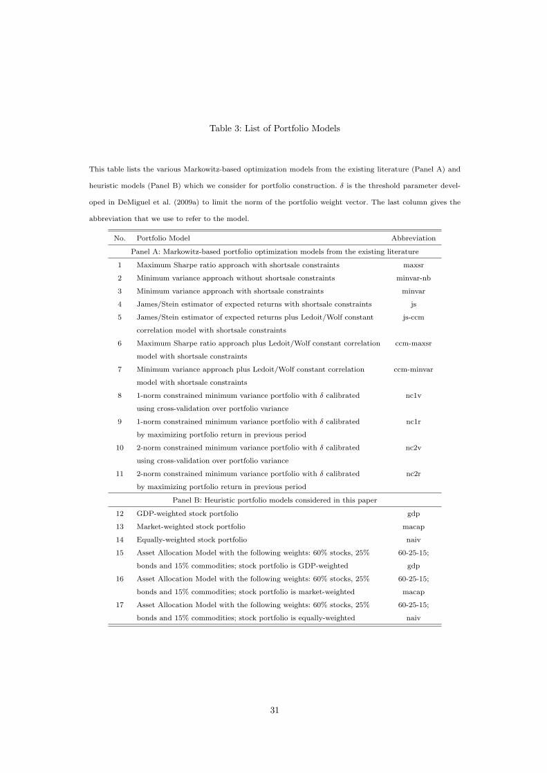
Table 3: List of Portfolio Models

This table lists the various Markowitz-based optimization models from the existing literature (Panel A) and

heuristic models (Panel B) which we consider for portfolio construction. δ is the threshold parameter devel-

oped in DeMiguel et al. (2009a) to limit the norm of the portfolio weight vector. The last column gives the

abbreviation that we use to refer to the model.

No. Portfolio Model Abbreviation

Panel A: Markowitz-based portfolio optimization models from the existing literature

1 Maximum Sharpe ratio approach with shortsale constraints maxsr

2 Minimum variance approach without shortsale constraints minvar-nb

3 Minimum variance approach with shortsale constraints minvar

4 James/Stein estimator of expected returns with shortsale constraints js

5 James/Stein estimator of expected returns plus Ledoit/Wolf constant js-ccm

correlation model with shortsale constraints

6 Maximum Sharpe ratio approach plus Ledoit/Wolf constant correlation ccm-maxsr

model with shortsale constraints

7 Minimum variance approach plus Ledoit/Wolf constant correlation ccm-minvar

model with shortsale constraints

8 1-norm constrained minimum variance portfolio with δ calibrated nc1v

using cross-validation over portfolio variance

9 1-norm constrained minimum variance portfolio with δ calibrated nc1r

by maximizing portfolio return in previous period

10 2-norm constrained minimum variance portfolio with δ calibrated nc2v

using cross-validation over portfolio variance

11 2-norm constrained minimum variance portfolio with δ calibrated nc2r

by maximizing portfolio return in previous period

Panel B: Heuristic portfolio models considered in this paper

12 GDP-weighted stock portfolio gdp

13 Market-weighted stock portfolio macap

14 Equally-weighted stock portfolio naiv

15 Asset Allocation Model with the following weights: 60% stocks, 25% 60-25-15;

bonds and 15% commodities; stock portfolio is GDP-weighted gdp

16 Asset Allocation Model with the following weights: 60% stocks, 25% 60-25-15;

bonds and 15% commodities; stock portfolio is market-weighted macap

17 Asset Allocation Model with the following weights: 60% stocks, 25% 60-25-15;

bonds and 15% commodities; stock portfolio is equally-weighted naiv

31

Tab

le4:

Mar

kow

itz

vs.H

euri

stic

s:In

tern

atio

nalSt

ock

Mar

ket

Div

ersi

ficat

ion

Res

ults

This

table

report

sm

eans,

standard

dev

iati

ons

and

Sharp

era

tios

of

month

lyout-

of-sa

mple

retu

rns

aft

erco

sts

as

wel

las

aver

age

turn

over

for

the

inte

rnati

onal

equity

port

folios

whic

hare

const

ruct

edusi

ng

the

vari

ous

Mark

ow

itz-

base

dopti

miz

ati

on

model

sand

heu

rist

icm

odel

s.Sharp

era

tios

are

report

edfo

rth

eto

tal

sam

ple

per

iod

(1973-2

008)

and

two

sub-s

am

ple

per

iods

(Feb

ruary

1973-J

anuary

1988

and

Feb

ruary

1988-D

ecem

ber

2008).

We

ass

um

ea

bid

-ask

spre

ad

of

40

basi

spoin

tsto

calc

ula

te

aft

er-c

ost

retu

rns.

The

last

colu

mns

giv

esth

ep-v

alu

esth

at

the

Sharp

era

tio

for

each

of

thes

em

odel

sis

diff

eren

tfr

om

that

for

the

GD

P-w

eighte

dst

ock

port

folio,

our

base

line

heu

rist

ic.W

eco

mpute

the

p-v

alu

esofth

ediff

eren

ceusi

ng

the

appro

ach

emplo

yed

by

DeM

iguel

etal.

(2009b)

and

atw

o-t

ailed

level

ofsi

gnifi

cance

.See

sect

ion

3

and

table

3fo

ra

des

crip

tion

ofth

em

odel

s.

Port

folio

Mea

nStd

.D

ev.

Mea

nA

nnual

Sharp

eR

ati

oSharp

eR

ati

oSharp

eR

ati

op-v

alu

e

Model

Ret

urn

Ret

urn

Turn

over

1973-2

008

1973-1

988

1988-2

008

H0

:S

R=

SR

gdp

PanelA

:M

arkow

itz-b

ase

dopti

miz

ati

on

models

maxsr

1.0

7%

5.7

9%

59.3

4%

0.1

06

0.1

21

0.0

99

0.9

7

min

var-

nb

0.9

3%

4.5

4%

30.7

0%

0.1

04

0.1

66

0.0

61

0.9

0

min

var

0.9

7%

4.5

9%

22.6

8%

0.1

12

0.1

66

0.0

75

0.7

2

js0.9

1%

5.0

2%

71.8

8%

0.0

89

0.1

21

0.0

67

0.4

7

js-c

cm0.9

0%

5.0

2%

66.9

5%

0.0

87

0.1

25

0.0

61

0.4

1

ccm

-maxsr

0.9

8%

5.5

5%

60.1

0%

0.0

93

0.1

25

0.0

76

0.6

0

ccm

-min

var

0.9

4%

4.5

8%

18.3

9%

0.1

06

0.1

58

0.0

70

0.9

4

nc1

v0.9

4%

4.5

4%

31.0

9%

0.1

06

0.1

66

0.0

65

0.9

7

nc1

r0.9

7%

4.5

7%

26.7

1%

0.1

13

0.1

66

0.0

76

0.7

4

nc2

v0.9

3%

4.5

6%

27.6

6%

0.1

03

0.1

66

0.0

59

0.8

0

nc2

r0.9

6%

4.5

7%

25.2

8%

0.1

09

0.1

66

0.0

70

0.8

8

PanelB

:H

euris

tic

models

gdp

0.9

7%

4.7

8%

11.2

7%

0.1

07

0.1

55

0.0

76

.

maca

p0.8

7%

4.7

5%

2.5

1%

0.0

87

0.1

57

0.0

40

0.0

6

naiv

0.9

9%

4.7

8%

12.9

2%

0.1

10

0.1

76

0.0

69

0.6

2

32

Tab

le5:

Mar

kow

itz

vs.H

euri

stic

s:A

sset

Allo

cati

onR

esul

ts

This

table

report

sm

eans,

standard

dev

iati

ons

and

Sharp

era

tios

ofm

onth

lyout-

of-sa

mple

retu

rns

aft

erco

sts

as

wel

las

aver

age

turn

over

for

the

ass

etalloca

tion

port

folios

whic

hare

const

ruct

edusi

ng

the

vari

ousM

ark

ow

itz-

base

dopti

miz

ati

on

model

sand

heu

rist

icm

odel

s.Sharp

era

tiosare

report

edfo

rth

eto

talsa

mple

per

iod

(1973-2

008)and

two

sub-s

am

ple

per

iods

(Feb

ruary

1973-J

anuary

1988

and

Feb

ruary

1988-D

ecem

ber

2008).

We

ass

um

ea

bid

-ask

spre

ad

of40

basi

spoin

tsto

calc

ula

teaft

er-c

ost

retu

rns.

The

last

colu

mns

giv

esth

ep-v

alu

esth

at

the

Sharp

era

tio

for

each

of

thes

em

odel

sis

diff

eren

tfr

om

that

for

the

60-2

5-1

5ass

etalloca

tion

port

folio

wit

hgdp-w

eighti

ng

inth

est

ock

mark

et,our

base

line

heu

rist

ic.W

eco

mpute

the

p-v

alu

esofth

ediff

eren

ceusi

ng

the

appro

ach

emplo

yed

by

DeM

iguel

etal.

(2009b)

and

atw

o-t

ailed

level

of

signifi

cance

.See

sect

ion

3and

table

3fo

ra

des

crip

tion

ofth

em

odel

s.

Port

folio

Mea

nStd

.D

ev.

Mea

nA

nnual

Sharp

eR

ati

oSharp

eR

ati

oSharp

eR

ati

op-v

alu

e

Model

Ret

urn

Ret

urn

Turn

over

1973-2

008

1973-1

988

1988-2

008

H0

:S

R=

SR

gdp

PanelA

:M

arkow

itz-b

ase

dopti

miz

ati

on

models

maxsr

0.8

3%

3.7

7%

49.7

1%

0.0

99

0.1

79

0.0

29

0.4

9

min

var-

nb

0.5

9%

1.1

4%

13.3

0%

0.1

21

0.1

67

0.0

81

0.8

8

min

var

0.6

2%

1.1

2%

7.3

5%

0.1

50

0.1

85

0.1

19

0.7

0

js0.7

4%

2.6

8%

41.1

0%

0.1

07

0.1

79

0.0

30

0.6

3

js-c

cm0.7

2%

2.7

2%

40.4

8%

0.0

97

0.1

86

0.0

08

0.4

4

ccm

-maxsr

0.6

9%

3.7

0%

51.0

1%

0.0

63

0.1

80

-0.0

34

0.1

2

ccm

-min

var

0.6

3%

1.1

4%

6.1

7%

0.1

51

0.1

82

0.1

26

0.6

6

nc1

v0.6

0%

1.1

3%

13.5

0%

0.1

23

0.1

68

0.0

84

0.9

1

nc1

r0.6

1%

1.1

2%

10.2

2%

0.1

40

0.1

63

0.1

21

0.8

4

nc2

v0.6

1%

1.1

3%

9.6

4%

0.1

32

0.1

85

0.0

86

0.9

6

nc2

r0.6

2%

1.1

2%

7.3

5%

0.1

50

0.1

85

0.1

19

0.7

0

PanelB

:H

euris

tic

models

60-2

5-1

5;gdp

0.8

8%

3.2

4%

12.7

2%

0.1

29

0.1

84

0.0

94

.

60-2

5-1

5;m

aca

p0.8

2%

3.2

1%

9.9

3%

0.1

13

0.1

85

0.0

63

0.0

8

60-2

5-1

5;naiv

0.8

9%

3.2

4%

13.3

9%

0.1

33

0.2

05

0.0

88

0.5

3

33

Table 6: Return Gaps of Various Indices compared to the GDP-weighted stock portfolio and the 60-25-15

asset allocation portfolio

This table reports the Sharpe ratio and Value-at-Risk at the 95% confidence level of monthly returns for

various indices as well as the GDP-weighted stock portfolio and the 60-25-15 asset allocation portfolio with

gdp-weighting in the stock market, which are our baseline heuristic models for portfolio construction. Moreover,

the table presents the Return Gap of these indices in basispoints (bp) per month compared to our baseline

heuristics. Portfolio weights are readjusted every February each year. See section 3 and table 3 for a description

of the models and subsection 4.1 for a description of the computation of the Return Gap.

Asset Class/ Sample Sharpe VaR 95% Return Gap Return Gap

Region Period Ratio (bp per month) (bp per month)

GDP-stock portfolio 60-25-15 portfolio

Panel A: Stock indices

MSCI Germany 73-08 0.097 -8.42% 4.2 10.3

MSCI France 73-08 0.098 -9.35% 3.6 9.8

MSCI Italy 73-08 0.059 -10.37% 24.7 24.2

MSCI United Kingdom 73-08 0.087 -9.02% 11.1 15.0

MSCI United States 73-08 0.083 -8.30% 12.6 16.0

MSCI Canada 73-08 0.074 -8.65% 16.3 18.5

MSCI Japan 73-08 0.056 -9.04% 24.7 24.2

MSCI Emerging Markets 88-08 0.098 -12.61% -10.5 -0.8

MSCI Europe 73-08 0.106 -7.75% 0.5 7.8

MSCI North America 73-08 0.086 -8.11% 10.8 14.8

MSCI Pacific 73-08 0.059 -8.61% 22.6 22.8

Panel B: Asset classes

GDP-stock portfolio 73-08 0.107 -7.91% . 7.5

Bonds 73-08 0.099 -1.29% 3.9 10.1

Commodities 73-08 0.074 -9.91% 15.5 18.0

34

Figure 1: Time-Series Behavior of Correlations within the Stock Market

This figure depicts the movement in the average correlation over the sample period for the regional stock

indices MSCI Europe, MSCI North America, MSCI Pacific and MSCI Emerging Markets with respect to

all other stock indices. Correlation coefficients are computed using a rolling window approach based on the

previous 60 months.

0

0,1

0,2

0,3

0,4

0,5

0,6

0,7

0,8

0,9

1

19

73

19

74

19

75

19

76

19

77

19

78

19

79

19

80

19

81

19

82

19

83

19

84

19

85

19

86

19

87

19

88

19

89

19

90

19

91

19

92

19

93

19

94

19

95

19

96

19

97

19

98

19

99

20

00

20

01

20

02

20

03

20

04

20

05

20

06

20

07

20

08

Europe

North America

Pacific

Emerging Markets

Figure 2: Time-Series Behavior of Correlations between Asset Classes

This figure depicts the movement in the average correlation over the sample period for the iBoxx Euro Overall

Index and the S&P GSCI Commodity Total Return Index with respect to the regional MSCI stock indices.

Correlation coefficients are computed using a rolling window approach based on the previous 60 months.

-0,6

-0,4

-0,2

0

0,2

0,4

0,6

0,8

1

19

73

19

74

19

75

19

76

19

77

19

78

19

79

19

80

19

81

19

82

19

83

19

84

19

85

19

86

19

87

19

88

19

89

19

90

19

91

19

92

19

93

19

94

19

95

19

96

19

97

19

98

19

99

20

00

20

01

20

02

20

03

20

04

20

05

20

06

20

07

20

08

iBoxx Euro Overall Bond Index

GSCI Commoditiy Index

35

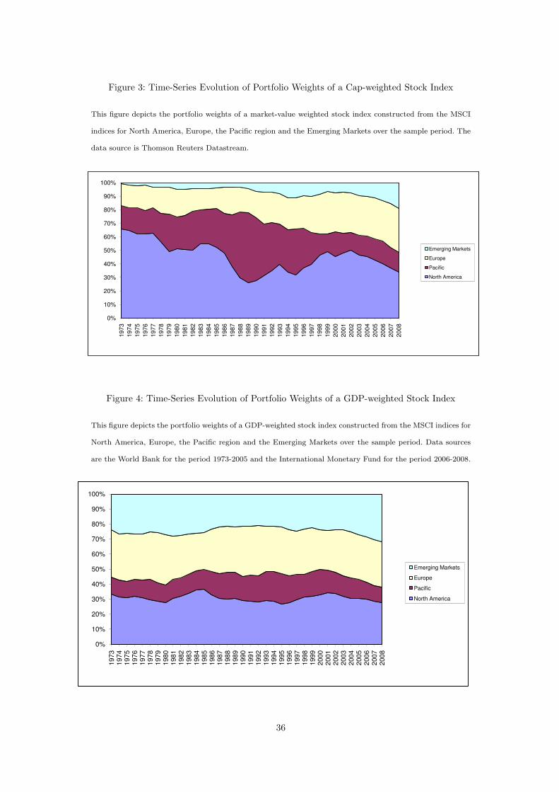
Figure 3: Time-Series Evolution of Portfolio Weights of a Cap-weighted Stock Index

This figure depicts the portfolio weights of a market-value weighted stock index constructed from the MSCI

indices for North America, Europe, the Pacific region and the Emerging Markets over the sample period. The

data source is Thomson Reuters Datastream.

0%

10%

20%

30%

40%

50%

60%

70%

80%

90%

100%

19

73

19

74

19

75

19

76

19

77

19

78

19

79

19

80

19

81

19

82

19

83

19

84

19

85

19

86

19

87

19

88

19

89

19

90

19

91

19

92

19

93

19

94

19

95

19

96

19

97

19

98

19

99

20

00

20

01

20

02

20

03

20

04

20

05

20

06

20

07

20

08

Emerging Markets

Europe

Pacific

North America

Figure 4: Time-Series Evolution of Portfolio Weights of a GDP-weighted Stock Index

This figure depicts the portfolio weights of a GDP-weighted stock index constructed from the MSCI indices for

North America, Europe, the Pacific region and the Emerging Markets over the sample period. Data sources

are the World Bank for the period 1973-2005 and the International Monetary Fund for the period 2006-2008.

0%

10%

20%

30%

40%

50%

60%

70%

80%

90%

100%

19

73

19

74

19

75

19

76

19

77

19

78

19

79

19

80

19

81

19

82

19

83

19

84

19

85

19

86

19

87

19

88

19

89

19

90

19

91

19

92

19

93

19

94

19

95

19

96

19

97

19

98

19

99

20

00

20

01

20

02

20

03

20

04

20

05

20

06

20

07

20

08

Emerging Markets

Europe

Pacific

North America

36

Figure 5: Graphical Presentation of the Performance of Alternative Fixed-Weight Asset Allocation Strate-

gies

This figure depicts the Sharpe ratios of alternative heuristic portfolio strategies in the asset allocation context.

In constructing the portfolios, we increase the portfolio weight of each asset class at the rebalancing date

in steps of 1% from 0% to 100% and adjust the portfolio weights of the other 2 classes appropriately. This

approach yields 5150 different portfolios. The stock component of the portfolios comprises the four regional

MSCI indices and is GDP-weighted.

020

4060

80100

020

4060

80100

00.020.040.060.08

0.10.120.140.160.18

0.2

Portfolio Weight BondsPortfolio Weight Stocks

Sharp

eR

ati

o

37