i

68404

Domestic Terms of Trade in Pakistan – Implications for

Agricultural Pricing and Taxation Policies

Safiya Aftab, Caesar Cororaton, Sohail Malik and Hans G.P. Jansen

Pub

lic D

iscl

osur

e A

utho

rized

Pub

lic D

iscl

osur

e A

utho

rized

Pub

lic D

iscl

osur

e A

utho

rized

Pub

lic D

iscl

osur

e A

utho

rized

Pub

lic D

iscl

osur

e A

utho

rized

Pub

lic D

iscl

osur

e A

utho

rized

Pub

lic D

iscl

osur

e A

utho

rized

Pub

lic D

iscl

osur

e A

utho

rized

ii

Executive Summary ..................................................................................................................................iii

I. Introduction ....................................................................................................................................... 1

II. Terms of Trade ................................................................................................................................. 1

III. Review of Literature .................................................................................................................. 3

III.1 Studies using weighted price indices .................................................................................... 3

III.2 Studies using indices of value added .................................................................................... 5

IV. Data and Methodology .............................................................................................................. 6

V. Results ................................................................................................................................................ 7

V.1 Terms of trade ............................................................................................................................... 7

V.1.1 Trends in agriculture’s terms of trade ....................................................................... 7

V.1.2 Poverty and economic impact of changing terms of trade ................................. 8

V.2 Agricultural income tax .......................................................................................................... 11

V.2.1 The agricultural income tax debate in Pakistan .................................................. 11

V.2.2 CGE model simulations ................................................................................................. 13

VI. Summary and Conclusions ................................................................................................... 17

References ................................................................................................................................................ 19

Annex I: Price Data .............................................................................................................................. 21

Annex II: Weights ................................................................................................................................ 23

Annex III: The CGE Model for Pakistan ....................................................................................... 26

AIII.1 Model functioning................................................................................................................ 26

AIII.2 Economic structure in the SAM and key model parameters ................................... 28

iii

Executive Summary

In 2008 the Government of Pakistan agreed with the IMF to increase the tax/GDP ratio

by 3.5 percentage points over the medium term. This commitment has rekindled the

debate regarding the agricultural income tax. Advocates of an agricultural income tax

argue that the sector remains protected by political interests, while opponents to such a

tax maintain that agriculture is already subject to significant indirect taxation, mainly

because of prevailing price distortions in agricultural product markets.

One way to assess agriculture’s performance in relation to other sectors of the economy is

to calculate the returns to the sector, relative to the payouts made by the sector. This

requires the construction of inter-sectoral terms of trade indices which allow comparison

of the value of “exports” from the agricultural sector to other sectors (mainly industry)

with “imports” from other sectors into agriculture.

This paper reviews the literature on domestic terms of trade analysis in Pakistan and

calculates an updated set of terms of trade indices for agriculture relative to industry. The

paper also discusses key issues with regard to the imposition of agricultural income tax in

Pakistan, and uses simulation results from a Computable General Equilibrium (CGE)

model for the Pakistan economy to analyze the potential effects of the imposition of an

agricultural income tax on poverty and fiscal revenues.

The results suggest that the domestic terms of trade have remained unfavorable for

Pakistan’s agriculture during almost the entire 2000-2009 period. Agriculture’s terms of

trade declined from 2001-02 to 2003-04 before improving only slightly during the period

from 2004-05 to 2006-07. As of 2007 however, prices of agricultural commodities

started rising resulting in significant increases in agriculture’s terms of trade. But in spite

of the substantial increases in agricultural prices, the terms of trade for agriculture,

though on a rising trend, remained marginally unfavorable to the sector.

A CGE model for Pakistan was used to simulate the poverty impacts of the declining

terms of trade for agriculture. During the period when agriculture’s terms of trade were

declining (1999-2000 to 2005-06), the volume of production in agriculture declined by

1.4 percent, while the volume of production in industry improved by 2.5 percent. Output

of the service sector declined by 0.8 percent. During the period when agriculture terms

of trade were improving (2005-06 to 2007-08), the output effects were largely the

reverse.

The same CGE model was also used to assess the poverty impacts of a hypothetical

agricultural income tax. Levying an income tax on large farmers (> 50 acres) was found

iv

to be pro-poor. A 6 percent income tax on this group would reduce the poverty incidence

only marginally (i.e. by -0.02 percent). However, a 30 percent income tax rate on large

farmers would reduce poverty by nearly 0.5 percent. Keeping total government

expenditure fixed in the model in order to assure model closure implies that higher

government revenues from increased direct tax revenue result in higher total savings in

the economy, which in turn leads to higher investment in especially the construction

sector. The latter increases its use of urban skilled and (especially) unskilled labor. Even

though agricultural output declines which has an adverse effect on rural poverty, the

decrease in urban poverty more than offsets the increase in rural poverty.

On the other hand, an agricultural tax imposed on medium farmers (12.5-50 acres) is not

generally pro-poor and may even increase poverty. This is because medium farmers

greatly outnumber large farmers and the initial poverty incidence among medium farmers

is much higher than among large farmers. On the other hand, while taxing both large and

medium farmers is not pro-poor, most simulations suggest that it does increase the tax

base relative to a tax on large farmers only. To the extent that the increased fiscal

revenues would be used to mitigate the poverty increase and the remainder for public

investments, taxing medium farmers could lead to certain social welfare gains. However,

to find out the exact effects would require more research and in the short-run taxation of

large farmers only seems to be the preferred option.

1

I. Introduction

Pakistan’s macroeconomic indicators significantly worsened during the 2006-08 period,

forcing the government to approach the IMF for assistance in November 2008. The

rapidly increasing fiscal deficit which reached 7.4 percent of GDP in FY2008 has been a

particular cause for concern. The agreement reached between the Government of

Pakistan (GoP) and the IMF requires the government to reduce the deficit to 4.2 percent

of GDP in FY2009 – a target that is to be achieved partly by increasing tax revenues by

0.6 percentage points of GDP (Government of Pakistan 2008, page 4). In the medium

term, the GoP has declared its intention to increasing the tax/GDP ratio by 3.5 percentage

points (Government of Pakistan 2008, page 7).

The government’s pledge to increase the tax/GDP ratio over the short, and then medium

term has rekindled a debate on the imposition of an agricultural income tax in the

country.1 This in turn, has led to a wider debate regarding taxation and pricing policy for

agriculture in general, with advocates of income tax on agricultural incomes arguing that

the sector remains protected by political interests, and opponents to additional taxation

maintaining that agriculture is subject to indirect taxation, mainly because of a pricing

structure that distorts the market for agricultural produce.

II. Terms of Trade

One way to assess the performance of the agriculture in relation to that of other sectors of

the economy is to calculate the returns to the sector, relative to the payouts the sector

makes. This requires the construction of an inter-sectoral terms of trade measure, where

the value of “exports” from the agricultural sector to other sectors (mainly industry) is

compared with “imports” from industry into agriculture. The value of the terms of trade

for any given year is thus calculated as the ratio of the value of the sector’s exports to the

value of its imports. More simply, the terms of trade index is constructed as the ratio of

the sector’s export price index and import price index. Most analysts use weighted and

normalized price indices to facilitate comparisons across time and across markets. Price

indices for terms of trade construction are often prepared using Laspeyre’s formula,

1 The “Panel of Economists” constituted by the government in early 2008 to design a stabilization plan for

Pakistan’s economy recommended “implementation of agricultural income tax by the provincial

governments” as one of the fiscal measures that the government should take, but did not assess the pros and

cons of the measure (see Government of Pakistan, 2009). The issue was raised in a meeting of the Senate’s

Standing Committee on 29 January 2009, but did not meet with much enthusiasm amongst the legislators,

most of whom vociferously opposed an income tax on agriculture. On the other hand, in a pre-budget

seminar conducted by the Association of Chartered Accountants on 3 May 2009 participants strongly

endorsed such a tax.

2

where the current values of the base period exports/imports are divided by the base period

values of the base period exports/imports.2

Calculation of inter-sectoral terms of trade indices enables analysts to determine how one

sector’s output is valued relative to another. A persistently unfavorable terms of trade

measure for a particular sector suggests that the sector’s output may be consistently

under-valued relative to the outputs of other sectors. Inter-sectoral terms of trade

measures are widely used for guidance in agricultural sector policy making. For example

in India the National Agricultural Policy states that the government will create a

favorable environment for the sector by endeavoring to improve the terms of trade of

agriculture with manufacturing.

Inter-sectoral terms of trade measures also reflect patterns of income distribution across

key sectors of the economy. Trends in the terms of trade can be indicative of the relative

growth in relevant sectors, and the analysis of such trends can thus have important policy

implications. In Pakistan, analysis of the terms of trade between agriculture and

manufacturing is particularly relevant as successive governments have been accused of

formulating policies which favor one sector to the detriment of the other. The GoP can

be expected to be interested in the debate around the terms of trade because of a

substantial proportion of legislators in the national and provincial legislatures who derive

some or all of their income from the agriculture sector. The need for robust estimation of

the inter-sectoral terms of trade is thus essential to facilitate a rational approach to policy-

making for the agriculture sector.

The remainder of this paper is structured as follows. The next section reviews the

literature on inter-sectoral terms of trade in Pakistan. Section IV explains the data and

methodology used in the analysis. Section V is the core of the paper and presents the

results, starting with an assessment of the relative competitiveness of the agricultural

sector by calculating an updated set of terms of trade for agriculture relative to industry.

This is followed by a discussion regarding the key issues with regard to the imposition of

agricultural income tax in Pakistan, based on simulation results from a Computable

General Equilibrium (CGE) model that is used to analyze the effects of the imposition of

such a tax on poverty and economic variables. Section VI concludes.

2 The scientific notation of the formula for Laspeyre’s index is given in Section IV (Data and

Methodology).

3

III. Review of Literature

Studies calculating the inter-sectoral terms of trade for Pakistan can broadly be divided

into two categories, i.e. (i) studies that employ weighted price indices to estimate

consumption of key goods in both sectors; and (ii) studies based on relative value added.

The first set consists of studies that are methodologically more rigorous, and these are

reviewed first.

III.1 Studies using weighted price indices

The first major study calculating the inter-sectoral terms of trade for Pakistan was by

Lewis and Hussain (1967) and covered the period 1951-64. They calculated two sets of

terms of trade indices (one for agriculture and the other for large-scale manufacturing)

and terms of trade were estimated separately for the then East and West Pakistan.

Wholesale price indices were used for three commodity groups, i.e. consumption goods,

intermediate goods and investment goods, and a weighting system was devised to

simulate inter-sectoral transactions. Regarding the latter, the authors first estimated the

net availability of goods in each category using a simple formula where availability was

defined as domestic supply plus imports minus exports. A set of assumptions on how the

goods produced in the agriculture and large-scale manufacturing sectors were absorbed

was adopted based on an estimation of the population in the two sectors. Alternative sets

of weights were derived assuming 10 percent, 25 percent and 40 percent lower

expenditure on non-agricultural consumption goods in the rural areas as compared to

urban areas. Intermediate and investment goods were assumed to have a higher

absorption rate in the non-agricultural sector.

Subsequently weighted price indices for exports from and imports into agriculture and

industry were constructed by multiplying wholesale price indices for specific

commodities by the estimated levels of consumption of these commodities in the

agriculture and industrial sectors. Agricultural goods consumed by the industry sector

were considered exports from agriculture, while industrial goods consumed in the

agriculture sector were considered imports into the agriculture sector.

The main results that the gross barter terms of trade for agriculture had deteriorated

during the period from 1951-52 to 1955-56, but then had improved steadily up to the mid

1960s.3 The improvement was especially significant in East Pakistan and the poor

performance of agriculture during the first half of the 1950s presumably reflected the

3 The gross barter terms of trade is the ratio (expressed as a percent) of a quantity index of exports from one

sector to a quantity index of inputs into that sector. In net barter terms of trade, volumes are held constant.

4

effects of the post-Korean war collapse in prices of raw materials in the early to mid-

1950s, coupled with an over-valued exchange rate. After 1955 however, the terms of

trade moved back in favor of agriculture because of the rapid industrial growth witnessed

in Pakistan over the period, which was partly fueled by the collapse in the prices of raw

materials in the mid 1950s.

The Lewis and Hussain study was updated a few years later by Lewis (1970) who only

calculated terms of trade indices for agriculture. The weighting scheme was changed

slightly to account for the increased production of wheat in West Pakistan and purchases

of fertilizer and machinery by the agriculture sector, data for which was obtained from

the national accounts. The key finding was that the terms of trade were favorable for

agriculture from 1964-67, but thereafter the value of the index declined, largely due to the

increased volume of agricultural production during the Green Revolution of the late

1960s which drove down agricultural prices. The 1970 Lewis study was updated by

Gotsch and Brown (1980) who used the same methodology to calculate a new set of

terms of trade indices. The main finding was a continuous, sharp decline in the terms of

trade for agriculture.

Kazi (1987) criticized the methodology used by Lewis and Hussain (1967), Lewis (1970)

and Gotsch and Brown (1980) arguing that the weighting scheme used in these studies

was based on arbitrary assumptions regarding the absorption of goods across sectors. In

particular Kazi argued that consumption was not likely to be proportionate to population;

that investment goods were unlikely to be purchased by stakeholders in the agriculture

sector; and that inclusion of only large-scale manufacturing outputs distorted the inter-

sectoral estimates. Expenditure on gas and electricity were highlighted as key services

used in the agriculture sector but not used in the studies mentioned.

Kazi (1987) calculated the inter-sectoral terms of trade for the period 1970-71 to 1981-82

using a new methodology for the construction of weights. The new weighting scheme

was based on household expenditure data from the Household Income and Expenditure

Survey (HIES) published by the Pakistan Federal Bureau of Statistics (FBS). The HIES

data included expenditures on major food items, fuel and lighting, as well as other

household expenditure categories, separated by urban and rural areas. These data were

disaggregated by percentages of the urban and rural populations engaged in agriculture

and non-agriculture, and used to estimate per capita consumption of agricultural and non-

agricultural goods by sections of the population engaged in agriculture or otherwise. The

results showed that the inter-sectoral terms of trade for the twelve year period under study

were generally in favor of agriculture, although there were sharp fluctuations in the

estimates over time.

5

Kazi’s methodology was in turn criticized by Qureshi (1987) who argued that weights

derived from estimates of consumer expenditure gives misleading results, as these are

based on response to retail rather than wholesale prices. Another criticism by Qureshi

concerned the range of commodities used in Kazi’s analysis which was smaller than in

Lewis’ 1970 study. As such Qureshi advocated the use of Lewis’ methodology because

of its superior coverage of commodities. Qureshi re-calculated the inter-sectoral terms of

trade for the period 1951-84 using Lewis’ methodology, with 1959-60 as the year base

for all individual price indices. In addition to the barter terms of trade, Qureshi’s study

also calculated the income and single factorial terms of trade.4 The main results

suggested that while the barter terms of trade for agriculture generally trended upward for

the period 1951-52 to 1983-84, the trend also concealed periods of sharp decline and

fluctuation. The decade wise analysis showed that the barter terms of trade for the

agriculture sector declined in the 1950s, rose sharply in the 1960s, fluctuated in the

1970s, and then declined again from 1977-78 to 1983-84.

III.2 Studies using indices of value added

A simpler, though methodologically less rigorous way of calculating inter-sectoral terms

of trade measures involves the use of implicit price indices from national accounts data.

This method was used by Cheong and D’Silva (1984) to calculate Pakistan’s inter-

sectoral terms of trade for the period 1960-83. GDP deflators for the agriculture and

manufacturing sectors were calculated by dividing current and constant value added in

these sectors, and then the inter-sectoral terms of trade was obtained as a ratio of these

deflators. The results suggested that the terms of trade between agriculture and the other

sectors did not significantly deteriorate over the period, and farmer’s purchasing power

gradually improved.

More recently, a set of inter-sectoral terms of trade indices were calculated using the

same methodology of estimating implicit price indices for the period 1970-71 to 2007-

08.5 The terms of trade obtained this way are consistently unfavorable for agriculture

throughout the entire period, with the exception of the year 1998-99 when value added in

minor crops registered a sharp increase. However, calculating inter-sectoral terms of

trade measures using implicit price indices from national accounts data is not robust and

therefore studies based on such methodology cannot be considered definitive.

4 The income terms of trade is the ratio (expressed as a percentage) of the value of exports from a sector to

the price of imports, while the single factorial terms of trade is the net barter terms of trade adjusted for

changes in the productivity of exports. 5 These unpublished estimates have been prepared by Dr. Abdus Salam at the Federal Urdu University,

Islamabad and are available upon request.

6

IV. Data and Methodology

Our study calculates inter-sectoral terms of trade for Pakistan’s agriculture using the

methodology outlined by Qureshi (see Qureshi 1987, pp. 38-41) but with some

modification in the weighting system. We used data regarding prices of selected

commodities included in the Social Accounting Matrix (SAM) from the most recent

issues of the Pakistan Economic Survey and Agricultural Statistics of Pakistan (see

Annex I for details). The data was then converted into indices using the year 2000-01 as

the base year.

The weights were derived from the SAM developed for Pakistan for 2001-02 by Dorosh

et al. (2006). This SAM is based on national income accounts data and the most recent

input-output table for Pakistan’s economy which dates from 1990-91. The weights used

consisted of the shares of different products in total value added in the Pakistan economy

in 2001-02, as derived from the SAM. The original SAM specified contribution to value

added for three sectors, agriculture, industry and services. However, since prices of

services are not listed in official statistical publications in Pakistan, the services sector

had to be left out of the analysis. Basically our analysis assumes that there are only two

sectors in the economy and that there is no leakage of goods outside these two sectors.

Even though this assumption is obviously a very strong one, there is no alternative at this

point in time.

Another constraint which forced us to consider only the agriculture and industry sectors

is that even though the SAM indicates the distribution of value added generated by

agriculture and industry across rural and urban populations, it does not do so for the

services sector. Therefore another (strong) assumption is that “rural” refers to agriculture

and “urban” refers to industry, with no further sub-division for services. The SAM

weights for the division of value added across commodities were modified to cover only

two sectors, agriculture and industry. The original weights of the SAM as well as the

modified weights are given in Annex II, respectively in Tables AII.1 and AII.2.

Once modified weights and price indices were prepared, the price indices for each

commodity were multiplied by the assigned weight to get the value of the commodity in

year j. The value calculated was thus PnQ0, with the value for year 2000-01 being the

base year value PoQ0. To distinguish between agriculture and industry we use the

notation PA

n, QA

0 and PM

n, QM

0, where QA

0 represents the weight assigned to a particular

commodity to denote its consumption in the agriculture sector, and QM

0 is the weight

assigned to each commodity to denote its consumption in the manufacturing sector. As

mentioned earlier, this division of each commodity’s consumption across agriculture and

7

manufacturing was derived from the division of income shares across rural and urban

areas as given in the SAM. Similarly, PA

n is the price of an agricultural commodity in

year n and PM

n is the price of an industrial good in year n.

The following index was derived for agricultural goods (k) consumed by the industrial

sector:

(1) k PA

kn QM

k0/k PA

k0 QM

k0 where k represents a summation across commodities

in one sector, in this case, agriculture.

A similar index was derived for industrial goods (i) consumed by the agriculture sector:

(2) i PM

in QA

i0/i PM

i0 QA

i0 where i represents a summation across commodities in

the other sector, in this case, industry.

The terms of trade for agriculture can then be calculated as the ratio of these two indices,

following the Laspeyre’s index formulation:

Terms of trade for agriculture = index of agricultural exports to industry/index of

agricultural imports from industry = (1) / (2) =

(3) (k PA

kn QM

k0/k PA

k0 QM

k0) / (i PM

in QA

i0/i PM

i0 QA

i0).

V. Results

V.1 Terms of trade

V.1.1 Trends in agriculture’s terms of trade

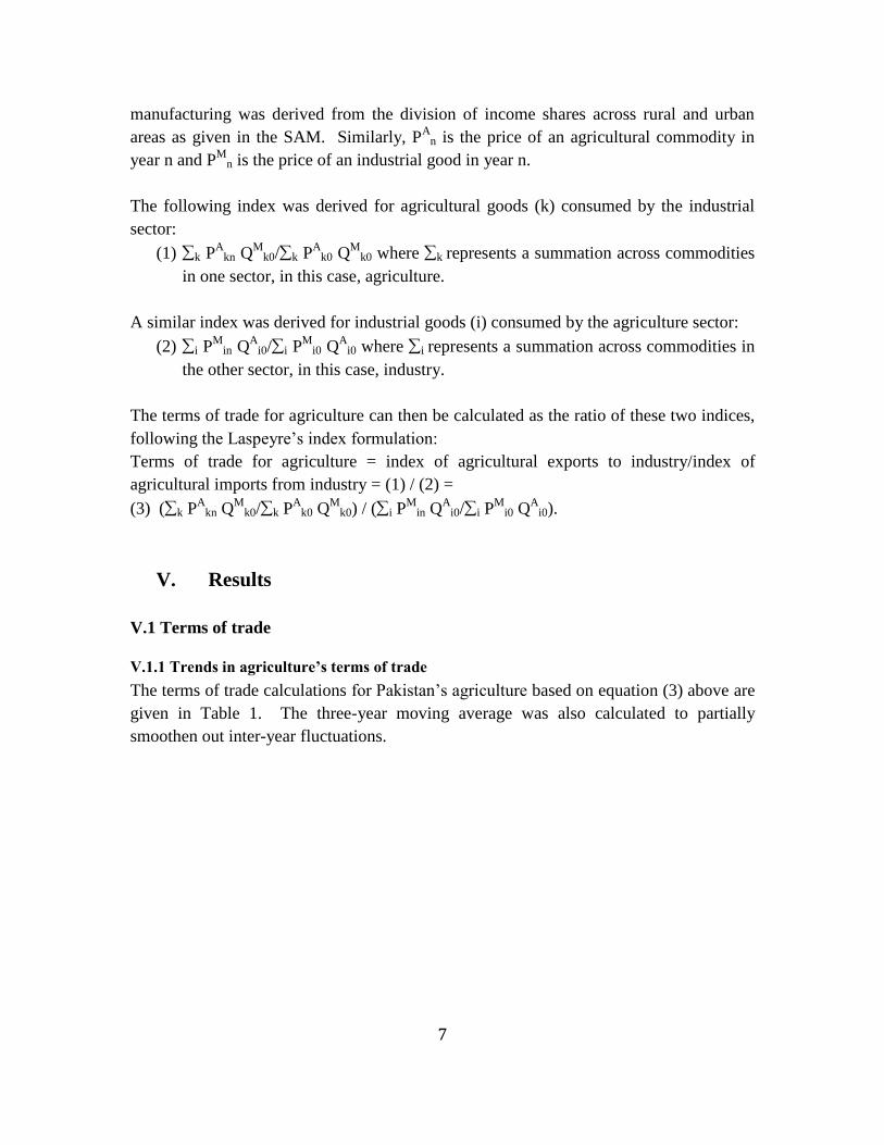
The terms of trade calculations for Pakistan’s agriculture based on equation (3) above are

given in Table 1. The three-year moving average was also calculated to partially

smoothen out inter-year fluctuations.

8

Table 1: Terms of trade for agriculture in Pakistan

Year Terms of Trade Terms of Trade

(three year moving average)

2000-01 100.00

2001-02 100.78 99.01

2002-03 96.24 95.63

2003-04 89.86 92.59

2004-05 91.68 91.28

2005-06 92.29 94.12

2006-07 98.40 96.58

2007-08 99.07

The terms of trade have remained unfavorable for Pakistan’s agriculture (i.e. consistently

below 100 for each year except 2001-02) for almost the entire period of analysis.

Moreover, agriculture’s terms of trade decreased between 2001-02 and 2003-04; and

improved slightly during 2004-06 before starting a significant upward trend thereafter,

largely as a result of the strong price increases of agricultural commodities that started in

2006-07. However and in spite of the substantial increases in food prices, the terms of

trade for agriculture remained marginally unfavorable to the sector. The three-year

moving average in Table 1 shows a similar trend with the terms of trade for agriculture

hitting its lowest point in 2004-05, and then showing some recovery for the two years that

follow, but remaining below parity.

V.1.2 Poverty and economic impact of changing terms of trade

A CGE model for Pakistan developed by Cororaton and Orden (2008) (see Annex III for

a description of the model) was used to assess the impact of changes in agriculture’s

terms of trade index6 for the period 1999-00 to 2007-08 on production, household

income, government revenue and poverty. Since agriculture’s terms of trade decreased

between 1999-00 and 2004-05 but increased between 2005-06 and 2007-08, the effects

during these two sub-periods were aggregated to arrive at the total effects for the entire

period 1999-00 and 2007-08. Given that terms of trade are computed using sectoral

prices and these prices are endogenous in the model, a sectoral production tax was

introduced in order to change the relative price between agriculture and non-agriculture.

6 The researchers used net barter terms of trade constructed by Dr. Abdus Salam at the Federal Urdu

University using the ratio of GDP deflators of the agriculture and industry sectors. These terms of trade

showed the same trends as the terms of trade calculated in this paper, and the simulation results with the

CGE model therefore remain relevant.

9

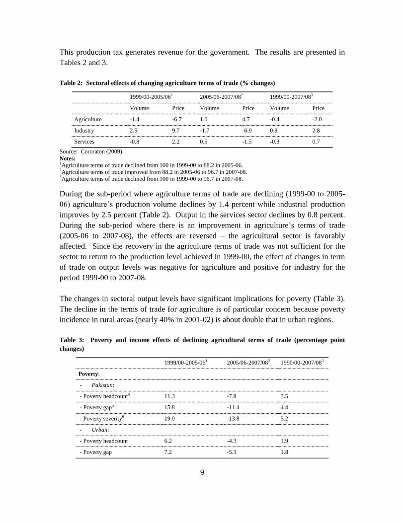
This production tax generates revenue for the government. The results are presented in

Tables 2 and 3.

Table 2: Sectoral effects of changing agriculture terms of trade (% changes)

1999/00-2005/061 2005/06-2007/082 1999/00-2007/083

Volume Price Volume Price Volume Price

Agriculture -1.4 -6.7 1.0 4.7 -0.4 -2.0

Industry 2.5 9.7 -1.7 -6.9 0.8 2.8

Services -0.8 2.2 0.5 -1.5 -0.3 0.7

Source: Cororaton (2009).

Notes: 1Agriculture terms of trade declined from 100 in 1999-00 to 88.2 in 2005-06. 2Agriculture terms of trade improved from 88.2 in 2005-06 to 96.7 in 2007-08. 3Agriculture terms of trade declined from 100 in 1999-00 to 96.7 in 2007-08.

During the sub-period where agriculture terms of trade are declining (1999-00 to 2005-

06) agriculture’s production volume declines by 1.4 percent while industrial production

improves by 2.5 percent (Table 2). Output in the services sector declines by 0.8 percent.

During the sub-period where there is an improvement in agriculture’s terms of trade

(2005-06 to 2007-08), the effects are reversed – the agricultural sector is favorably

affected. Since the recovery in the agriculture terms of trade was not sufficient for the

sector to return to the production level achieved in 1999-00, the effect of changes in term

of trade on output levels was negative for agriculture and positive for industry for the

period 1999-00 to 2007-08.

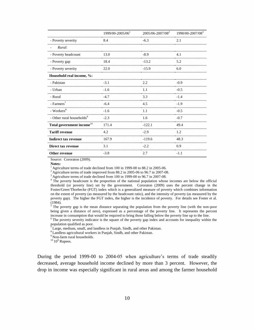
The changes in sectoral output levels have significant implications for poverty (Table 3).

The decline in the terms of trade for agriculture is of particular concern because poverty

incidence in rural areas (nearly 40% in 2001-02) is about double that in urban regions.

Table 3: Poverty and income effects of declining agricultural terms of trade (percentage point

changes)

1999/00-2005/061 2005/06-2007/082 1990/00-2007/083

Poverty:

- Pakistan:

- Poverty headcount4 11.3 -7.8 3.5

- Poverty gap5 15.8 -11.4 4.4

- Poverty severity6 19.0 -13.8 5.2

- Urban:

- Poverty headcount 6.2 -4.3 1.9

- Poverty gap 7.2 -5.3 1.8

10

1999/00-2005/061 2005/06-2007/082 1990/00-2007/083

- Poverty severity 8.4 -6.3 2.1

- Rural:

- Poverty headcount 13.0 -8.9 4.1

- Poverty gap 18.4 -13.2 5.2

- Poverty severity 22.0 -15.9 6.0

Household real income, %:

- Pakistan -3.1 2.2 -0.9

- Urban -1.6 1.1 -0.5

- Rural -4.7 3.3 -1.4

- Farmers7 -6.4 4.5 -1.9

- Workers8 -1.6 1.1 -0.5

- Other rural households9 -2.3 1.6 -0.7

Total government income10 171.4 -122.1 49.4

Tariff revenue 4.2 -2.9 1.2

Indirect tax revenue 167.9 -119.6 48.3

Direct tax revenue 3.1 -2.2 0.9

Other revenue -3.8 2.7 -1.1

Source: Cororaton (2009).

Notes: 1 Agriculture terms of trade declined from 100 in 1999-00 to 88.2 in 2005-06. 2 Agriculture terms of trade improved from 88.2 in 2005-06 to 96.7 in 2007-08. 3 Agriculture terms of trade declined from 100 in 1999-00 to 96.7 in 2007-08.

4 The poverty headcount is the proportion of the national population whose incomes are below the official

threshold (or poverty line) set by the government. Cororaton (2009) uses the percent change in the

Foster/Greer/Thorbecke (FGT) index which is a generalized measure of poverty which combines information

on the extent of poverty (as measured by the headcount ratio), and the intensity of poverty (as measured by the

poverty gap). The higher the FGT index, the higher is the incidence of poverty. For details see Foster et al.

(1984). 5 The poverty gap is the mean distance separating the population from the poverty line (with the non-poor

being given a distance of zero), expressed as a percentage of the poverty line. It represents the percent

increase in consumption that would be required to bring those falling below the poverty line up to the line. 6 The poverty severity indicator is the square of the poverty gap index and accounts for inequality within the

population qualified as poor. 7 Large, medium, small, and landless in Punjab, Sindh, and other Pakistan. 8 Landless agricultural workers in Punjab, Sindh, and other Pakistan. 9 Non-farm rural households. 10 109 Rupees.

During the period 1999-00 to 2004-05 when agriculture’s terms of trade steadily

decreased, average household income declined by more than 3 percent. However, the

drop in income was especially significant in rural areas and among the farmer household

11

category in particular.7 This also led to an increase in the overall poverty headcount rate

of more than 11 percent (and even higher in rural areas). On the other hand, during the

period of improving agricultural terms of trade (2005-06 to 2007-08) household incomes

also improved, especially in rural areas. As a result the overall poverty incidence

decreases by 7.8 percent and by nearly 9 percent in rural areas. However, the favorable

poverty effect during this period is not sufficient to offset the increases in poverty

suffered during the period of worsening agricultural terms of trade. Thus, considering the

entire period between 1999-00 and 2007-08, poverty increased by 3.5 percent.

The agricultural lobby in Pakistan (mostly consisting of large landowners) has

consistently argued that the agriculture sector is at a disadvantage compared to industry,

at least with regard to its pricing structure. The terms of trade analysis in this section

seems to support the argument. A key question now becomes the following: To what

extent does the relative disadvantage of the agricultural sector vis-à-vis the industry

sector affect the case for imposition of agricultural income tax? This issue is the main

topic of discussion in the next section.

V.2 Agricultural income tax

V.2.1 The agricultural income tax debate in Pakistan

Agricultural income is exempt from federal income tax as per the Federal Income Tax

Ordinance 2001, although agricultural output continues to be taxed through the land

revenue system.8 Since the early 1990s when Pakistan began implementation of a series

of structural adjustment program with the IMF, the country has become under increasing

pressure to institute a tax on agricultural income. However the issue whether or not

agricultural income should be subject to taxation has historically been a very contentious

one: Pakistan’s legislature is largely populated by members of rural landowning

families,9 and many of them derive a significant proportion of their income and wealth

from agriculture. As such, there has traditionally been strong opposition against the

introduction of an agricultural income tax.

7 Overall household income declines, because changes in sectoral terms of trade were simulated using a

production tax which also increases government revenue. 8 The prime form of agricultural output taxation at the provincial level is the imposition of Ushr based on

an estimated and standardized production volume by type of farm. Ushr is passed on by the provincial

government to the local Zakats (or charity committees) and does not show up in the provincial

government’s revenue records. In addition, North West Frontier Province (NWFP) imposes a land revenue

cess on the basis of area of land owned. 9 According to the Economist Intelligence Unit’s 2001-02 Country Report for Pakistan, 70 percent of

legislators who were elected to sit on local bodies in the 2001 elections could be classified as “rural gentry”

based on the size of their declared landholdings.

12

The main arguments of legislators as well as some policy makers against an agricultural

income tax are twofold. First, Pakistan’s policy regime has traditionally been biased

against agriculture and that the sector is subject to excessive price regulation. These

price controls, so the argument goes, are a form of implicit taxation and effectively

ensure that the inter-sectoral terms of trade remain biased against agriculture.10

Second,

agricultural income is acknowledged to be highly variable in nature, and opponents of an

agricultural income tax argue that its taxation would increase administrative costs to a

degree not compatible with the eventual yield of the tax.11

The only form in which an

agricultural income tax would be collectible, the argument goes, is in the form of a

modified land tax. However, such a formulation of an agricultural income tax would be

just as regressive as the current land taxation system and would therefore defeat the

equity purpose of such a tax.

A number of economists and policymakers have expressed disagreement with the above

arguments against the introduction of an agricultural income tax, and have put forward

four counterarguments. The first is that it is fundamentally illogical to make a distinction

between incomes from different sources when imposing any form of taxation on income.

According to internationally accepted jurisprudence taxes are levied on individuals and

not on sectors: therefore there can be no distinction between the income an individual

earns from agricultural landholdings, and the income he/she earns from other sources.

Second, incomes below a minimum level would be exempt from agricultural income

taxation since they are exempt from income tax in general. Therefore an agricultural

income tax would not have an adverse effect on poor farmers. Third, an agricultural

income tax that would primarily target large farmers is justified from a social point of

view since it would tax those who have traditionally benefited the most from the various

subsidies and other incentives provided by the government to the sector. Finally, the

current exemption from taxation accorded to income from agriculture creates

opportunities for tax evasion and fraud. While the agriculture sector contributes about

one-fifth to total GDP, tax collection from agriculture in Pakistan is minuscule

The debate has been continuing for over a decade now and indeed in three provincial

governments (Punjab, Sindh and NWFP) there exists a (weak) form of agricultural

10

Agricultural pricing policy in Pakistan historically tended to focus on keeping food prices down for urban

consumers, with the underlying assumption that farmers are not responsive to crop prices in any case.

These policies began to be reviewed with increased liberalization of the economy from the early 1990s

onwards, but price setting in the agriculture sector remains a controversial issue. 11

Here the argument is that imposing tax on a highly innumerate rural population which traditionally does

not maintain accounts would be a waste of administrative resources.

13

income tax (AIT) since 2001.12

However, in all three provinces the tax is levied largely

as a presumptive tax and collected by the Board of Revenue whose main responsibility is

the collection of land taxes.13

The yield from the presumptive tax is far below potential –

recent studies have estimated that revenue collection from this tax in the Punjab should

be four times the amount actually collected while in NWFP, it should be ten times the

current amounts (Malik 2004, Bahl et al. 2007).14

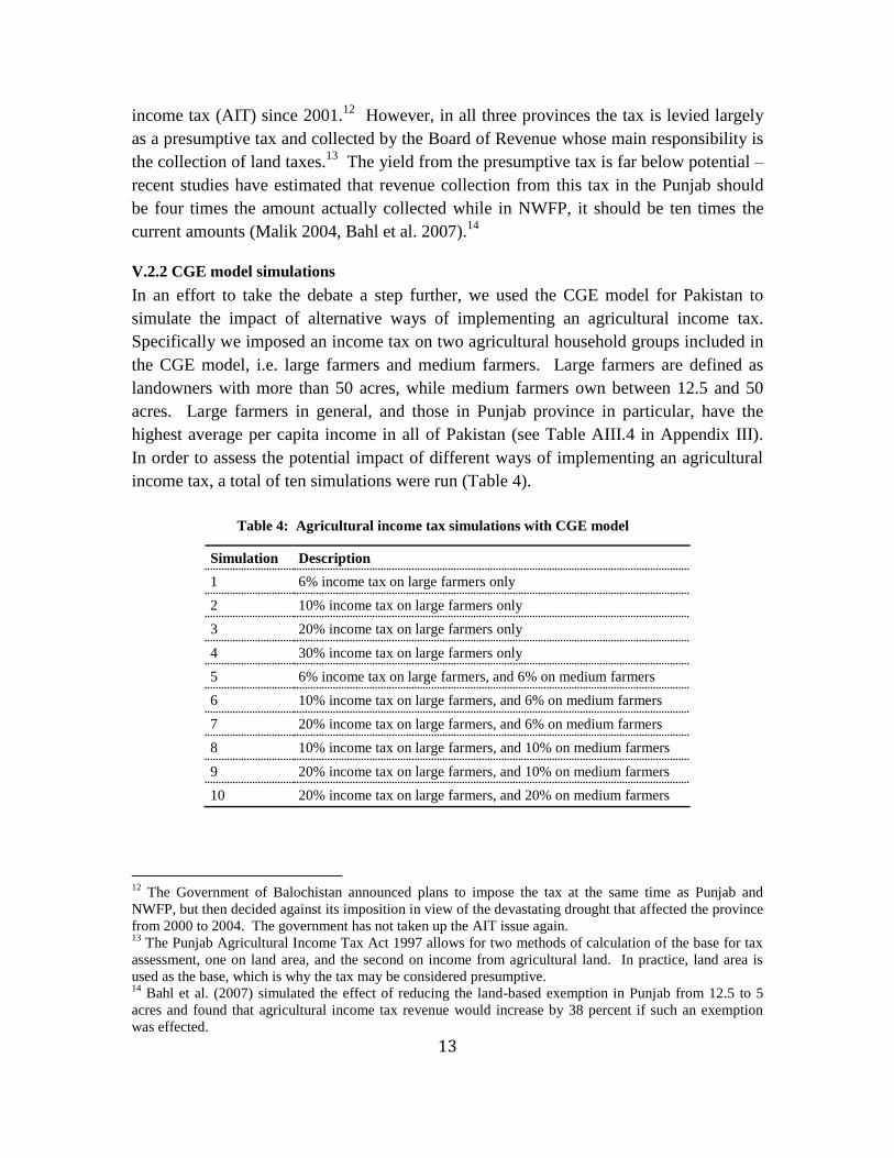
V.2.2 CGE model simulations

In an effort to take the debate a step further, we used the CGE model for Pakistan to

simulate the impact of alternative ways of implementing an agricultural income tax.

Specifically we imposed an income tax on two agricultural household groups included in

the CGE model, i.e. large farmers and medium farmers. Large farmers are defined as

landowners with more than 50 acres, while medium farmers own between 12.5 and 50

acres. Large farmers in general, and those in Punjab province in particular, have the

highest average per capita income in all of Pakistan (see Table AIII.4 in Appendix III).

In order to assess the potential impact of different ways of implementing an agricultural

income tax, a total of ten simulations were run (Table 4).

Table 4: Agricultural income tax simulations with CGE model

Simulation Description

1 6% income tax on large farmers only

2 10% income tax on large farmers only

3 20% income tax on large farmers only

4 30% income tax on large farmers only

5 6% income tax on large farmers, and 6% on medium farmers

6 10% income tax on large farmers, and 6% on medium farmers

7 20% income tax on large farmers, and 6% on medium farmers

8 10% income tax on large farmers, and 10% on medium farmers

9 20% income tax on large farmers, and 10% on medium farmers

10 20% income tax on large farmers, and 20% on medium farmers

12

The Government of Balochistan announced plans to impose the tax at the same time as Punjab and

NWFP, but then decided against its imposition in view of the devastating drought that affected the province

from 2000 to 2004. The government has not taken up the AIT issue again. 13

The Punjab Agricultural Income Tax Act 1997 allows for two methods of calculation of the base for tax

assessment, one on land area, and the second on income from agricultural land. In practice, land area is

used as the base, which is why the tax may be considered presumptive. 14

Bahl et al. (2007) simulated the effect of reducing the land-based exemption in Punjab from 12.5 to 5

acres and found that agricultural income tax revenue would increase by 38 percent if such an exemption

was effected.

14

The results of the simulations are presented in Table 5. The main result is that imposing

an agricultural income tax on large farmers is pro-poor. This can be explained as

follows: keeping total government expenditure fixed in the model in order to assure

model closure implies that higher government revenues from increased direct tax revenue

result in higher total savings in the economy, which in turn leads to higher investments,

especially in the construction sector. The latter increases its use of urban skilled and

(especially) unskilled labor. Even though agricultural output declines which has an

adverse effect on rural poverty, the decrease in urban poverty more than offsets the

increase in rural poverty.

Whereas a 6 percent agricultural income tax on large farmers would reduce the overall

poverty incidence only marginally (by 0.02 percent), a 30 percent tax rate reduces

poverty by nearly one-half percent. Overall real income of households slightly declines

but there is a redistribution of income from farmers (particularly large farmers) to the rest

of the household groups. Also, the agricultural income tax increases the tax base (Table

5). When the tax is levied on large farmers only, the increase in government revenues

varies from Rs 6 billion in simulation # 1 (6 percent income tax) to Rs 32.1 billion in

simulation # 6 (30 percent income tax).

Thus, while the poverty-reducing effect of such a tax may be less than spectacular, the

more important point is that the results demystify the arguments of some opponents to the

tax who argue that taxing agricultural incomes would lead to an increase in overall

poverty.

Simulations #s 5 to 10 represent various combinations of income tax rates on large

farmers and medium farmers. Except for simulation # 7 (representing a 20 percent

income tax on large farmers and 6 percent on medium farmers) the results are not

generally pro-poor.15

The overall poverty incidence also increases, mainly because the

number of medium farmers greatly exceeds the number of large farmers and the poverty

incidence among medium farmers is also much higher than in large farmers. Taxing both

large and medium farmers at the same time implies a redistribution of income from these

two groups of farmers to the other household groups.

Finally, it is worth noting that while imposition of an income tax on both large and

medium farmers is not pro-poor, most simulations suggest that it does increase the tax

base relative to a tax on large farmers only. For example when the income of both groups

15

As a matter of fact even simulation # 7 would lead to increased rural poverty but this increase is more

than offset by the decrease in urban poverty.

15

Table 5: Simulation results

Simulations a

1 2 3 4 5 6 7 8 9 10

Poverty: Base:

2001-02 Index

Pakistan % change from base

Poverty headcount 31.2 -0.02 -0.14 -0.32 -0.48 0.18 0.07 -0.09 0.41 0.09 0.89

Poverty gap 6.5 -0.13 -0.20 -0.33 -0.45 0.23 0.16 0.02 0.61 0.46 2.34

Poverty severity 2.0 -0.17 -0.25 -0.33 -0.21 0.23 0.15 0.06 0.71 0.62 3.60

Urban

Poverty headcount 19.9 -0.10 -0.19 -0.57 -0.76 -0.57 -0.57 -0.95 -0.95 -1.52 -1.90

Poverty gap 3.9 -0.20 -0.33 -0.66 -0.98 -0.71 -0.83 -1.15 -1.16 -1.47 -2.24

Poverty severity 1.2 -0.23 -0.39 -0.77 -1.14 -0.82 -0.97 -1.34 -1.35 -1.71 -2.61

Rural

Poverty headcount 38.2 0.00 -0.12 -0.24 -0.39 0.42 0.27 0.18 0.84 0.60 1.78

Poverty gap 8.0 -0.10 -0.15 -0.23 -0.29 0.51 0.45 0.37 1.13 1.04 3.71

Poverty severity 2.5 -0.15 -0.21 -0.20 0.06 0.53 0.47 0.46 1.30 1.29 5.38

Real incomes: 2001-02

population

distribution (%)

% change from base

Pakistan 100 -0.13 -0.22 -0.43 -0.64 -0.46 -0.54 -0.76 -0.76 -0.97 -1.50

Urban 28.6 0.05 0.09 0.18 0.27 0.19 0.23 0.32 0.32 0.41 0.64

Urban poor 8.1 0.05 0.08 0.16 0.24 0.17 0.21 0.28 0.29 0.36 0.56

Rural 71.4 -0.34 -0.57 -1.14 -1.70 -1.16 -1.39 -1.95 -1.93 -2.49 -3.82

Farmers b 34.2 -0.60 -1.01 -2.01 -3.01 -2.06 -2.46 -3.45 -3.42 -4.41 -6.79

16

Simulations a

1 2 3 4 5 6 7 8 9 10

Workers c 6.6 0.07 0.11 0.23 0.34 0.24 0.29 0.41 0.41 0.53 0.83

Other rural households d 30.7 0.04 0.06 0.12 0.19 0.13 0.16 0.22 0.22 0.29 0.46

Government revenues: Base: 2001-02

SAM e

Change from base (billion rupees)

Fiscal balance -8.5 6.4 10.7 21.4 32.1 22.0 26.2 36.9 36.6 47.3 73.1

Total government income 446.1 6.4 10.7 21.4 32.1 22.0 26.2 36.9 36.6 47.3 73.1

Tariff revenue 48.1 0.1 0.1 0.3 0.4 0.3 0.3 0.5 0.5 0.6 0.9

Indirect tax revenue 219.8 0.7 1.2 2.3 3.5 2.5 2.9 4.1 4.1 5.3 8.4

Direct tax revenue 146.2 5.7 9.5 18.9 28.4 19.4 23.1 32.6 32.2 41.7 64.3

Other revenue 32.0 0.0 -0.1 -0.1 -0.2 -0.1 -0.2 -0.2 -0.2 -0.3 -0.5

a For definition of simulations see Table 4. b Large, medium, small, and landless in Punjab, Sindh, and other Pakistan.

c Landless agricultural workers in Punjab, Sindh, and other Pakistan. d Non-farm rural households. e 109 Rupees.

17

is taxed at a rate of 20 percent (simulation # 10), fiscal revenues increase by Rs 73.1

billion.

VI. Summary and Conclusions

This paper has updated the terms of trade index for Pakistan’s agriculture sector, using a

new weighting scheme. This scheme, based on estimates of distribution of value added

in Pakistan’s economy across key activities, is methodologically superior to traditional

methods of weighting used in earlier studies, which were for the most part based on the

assumption that total consumption in the economy is distributed according to the

distribution of population. The newly constructed terms of trade measure shows a

declining trend between 2000 and 2005 but an upward trend thereafter. This trend

reversal is primarily due to the significant food price increases seen after 2006 in Pakistan

(as in most other countries). However, it is important to note that in spite of this trend

reversal, the terms of trade for agriculture relative to industry has thus far failed to

achieve parity.

A recently developed CGE model for Pakistan was used to assess the potential effects of

an agricultural income tax on poverty and fiscal revenue. A total of ten different

simulations representing alternative tax regimes were performed and the results tell an

interesting story. The imposition of an agricultural income tax on large farmers only is

unambiguously poverty reducing, in addition to significantly increasing public revenue.

Moreover, since the CGE model used was a static model and therefore does not take into

account second and third round effects, there may be additional poverty reducing effects

depending on how the additional fiscal revenue is utilized. Inclusion of medium farmers

in an agricultural income tax scheme would likely increase the poverty headcount and

therefore would be difficult to recommend. On the other hand it would also greatly

increase fiscal revenues and to the extent that part of the latter would be used to mitigate

the poverty increase and the remainder for public investments, taxing medium farmers

could lead to certain social welfare gains. However, to find out the exact effects would

require more research and in the short-run taxation of large farmers only seems the

preferred option.

Finally, there is a clear need for increased efforts in data generation, modeling and

agricultural policy analysis in Pakistan. The SAM that underlies the CGE model used in

this paper dates back to 2001-02 and needs updating. More researchers need to be trained

in CGE analysis and other modeling techniques which can provide important insights into

the behavior of economic variables. Policy making in Pakistan is often conducted in a

vacuum, dependent on anecdotal evidence and (political) opinions rather than guided by

18

quantitative analysis – a trend that should be reversed if agricultural policy is to become

more effective and credible at the same time.

19

References

Bahl, R., S. Wallace and M. Cyan (2007). Pakistan Provincial Government Study.

Unpublished background paper for the 2008 Pakistan Tax Policy Report being prepared

by the Federal Board of Revenue in collaboration with the World Bank. Islamabad.

Cheong, K.C. and E.H. D’Silva (1984). Prices, Terms of Trade and the Role of

Government in Pakistan's Agriculture. World Bank Staff Working Paper No. 643.

Washington D.C.

Cororaton, B.C. and D. Orden (2008). Pakistan’s Cotton and Textile Economy:

Intersectoral Linkages and Effects on Rural and Urban Poverty. IFPRI Research Report

No. 158. Washington, D.C.: International Food Policy Research Institute.

Cororaton, B.C. (2009). Note on the Results of the CGE Model for Pakistan.

International Food Policy Research Institute (IFPRI), Washington, D.C. Unpublished.

Dorosh, P., M.K. Niazi and H. Nazli (2006). A Social Accounting Matrix for Pakistan,

2001-02: Methodology and Results. PIDE Working Papers 2006, No. 9. Pakistan

Institute of Development Economics, Islamabad.

Foster, J., J. Greer and E. Thorbecke (1984). A class of decomposable poverty measures.

Econometrica (52): 761-766.

Gotsch, C.H. and G. Brown (1980). Prices, Taxes and Subsidies in Pakistan’s

Agriculture, 1960-75. World Bank Staff Working Paper No. 387. Washington D.C.

Government of Pakistan (2008). Letter of Intent from the Government of Pakistan to the

International Monetary Fund, November 20, 2008.

Kazi, S. (1987). Inter-sectoral Terms of Trade for Pakistan’s Economy 1970-71 to 1981-

82. Pakistan Development Review XXVII (2) (Spring).

Lewis, S.R. (1970). Agriculture’s Terms of Trade. Pakistan Development Review X (3).

(Autumn).

Lewis, S.R. and S.M. Hussain (1967). Relative Price Changes and Industrialization in

Pakistan 1951-64. Pakistan Institute of Development Economics (PIDE), Monograph

No. 16. Karachi.

20

Malik, S. (2004). Study on Tax Potential in NWFP. Innovative Development Strategies,

Ltd. Mimeographed. Islamabad.

Government of Pakistan (2009). Interim Report on Stabilization with a Human Face.

Report of the Panel of Economists for the Planning Commission. Islamabad.

Qureshi, S.K. (1987). Agricultural Pricing and Taxation in Pakistan – Some Policy

Issues. Pakistan Institute of Development Economics (PIDE). Islamabad.

State Bank of Pakistan (2008). Annual Report. Karachi.

21

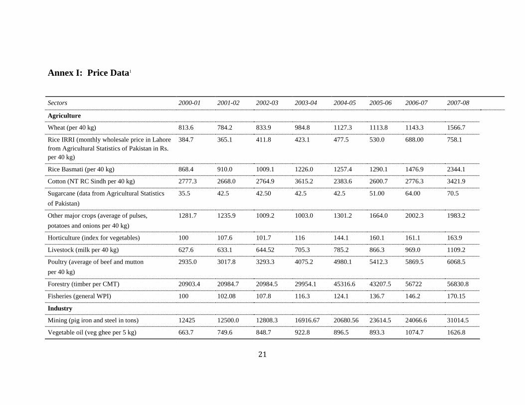
Annex I: Price Data1

Sectors 2000-01 2001-02 2002-03 2003-04 2004-05 2005-06 2006-07 2007-08

Agriculture

Wheat (per 40 kg) 813.6 784.2 833.9 984.8 1127.3 1113.8 1143.3 1566.7

Rice IRRI (monthly wholesale price in Lahore

from Agricultural Statistics of Pakistan in Rs.

per 40 kg)

384.7 365.1 411.8 423.1 477.5 530.0 688.00 758.1

Rice Basmati (per 40 kg) 868.4 910.0 1009.1 1226.0 1257.4 1290.1 1476.9 2344.1

Cotton (NT RC Sindh per 40 kg) 2777.3 2668.0 2764.9 3615.2 2383.6 2600.7 2776.3 3421.9

Sugarcane (data from Agricultural Statistics

of Pakistan)

35.5 42.5 42.50 42.5 42.5 51.00 64.00 70.5

Other major crops (average of pulses,

potatoes and onions per 40 kg)

1281.7 1235.9 1009.2 1003.0 1301.2 1664.0 2002.3 1983.2

Horticulture (index for vegetables) 100 107.6 101.7 116 144.1 160.1 161.1 163.9

Livestock (milk per 40 kg) 627.6 633.1 644.52 705.3 785.2 866.3 969.0 1109.2

Poultry (average of beef and mutton

per 40 kg)

2935.0 3017.8 3293.3 4075.2 4980.1 5412.3 5869.5 6068.5

Forestry (timber per CMT) 20903.4 20984.7 20984.5 29954.1 45316.6 43207.5 56722 56830.8

Fisheries (general WPI) 100 102.08 107.8 116.3 124.1 136.7 146.2 170.15

Industry

Mining (pig iron and steel in tons) 12425 12500.0 12808.3 16916.67 20680.56 23614.5 24066.6 31014.5

Vegetable oil (veg ghee per 5 kg) 663.7 749.6 848.7 922.8 896.5 893.3 1074.7 1626.8

22

Sectors 2000-01 2001-02 2002-03 2003-04 2004-05 2005-06 2006-07 2007-08

Wheat milling (flour retail price per kg) 9.8 9.7 10.1 11.7 13.28 13.1 13.6 18.07

Rice milling IRRI (retail per kg) 11.6 11.5 12.2 13.1 15.42 16.05 17.59 29.32

Rice milling basmati (retail per kg) 15.4 15.5 18.1 19.0 20.19 20.2 23.11 37.77

Sugar (per 40 kg) 1317.0 1077.7 988.5 885.0 1113.12 1577.3 1552.5 1290.8

Other food (wholesale price index for food) 100 102.1 105.6 113.0 125.0 133.8 145.7 173.28

Lint, yarn (Sindh Fin Bridge per 5 kg) 465.0 438.0 479.4 582.9 525.4 537.5 550.6 550

Textiles (kohinoor per meter) 800 820 820 1478.5 1680.8 1675.8 1711.6 1740

Leather (index 2001-02=100) 100 100 95.2 93.6 102.77 110.65 111.9 121.84

Wood (CPI for household furniture and

equipment)

100 103.9 106.9 110.7 117.34 123.41 131.649 141.08

Chemicals (caustic soda solid per 50kg) 1304.1 1764.2 1578.6 1415.8 1472.0 1749.1 1619.9 2066.7

Cement (Zeal Pak tons) 3824.2 3809.1 3951.8 4190.7 4190.7 5059.2 5285 4775

Petroleum (motor spirit bulk in liters) 30.7 31.56 32.75 34.1 41.3 55.6 55.6 59.1

Other manufacturing (wholesale price index

for manufacturing)

100.0 101.91 103.67 111.8 113.1 115.4 119.9 128.3

Energy (wholesale price index for fuel,

lighting and lubricants)

100.0 103.1 116.0 119.2 138.0 174.6 184.1 223.3

Source: Unless mentioned otherwise, data is from the Pakistan Economic Survey 2007-08. Data on prices of rice (IRRI varieties) and sugarcane is from Agricultural Statistics of

Pakistan 2004-05 and 2006-07. Data for 2007-08 for these two commodities was extrapolated using average annual growth rates.

Note: 1 Text in brackets gives the unit in which price is recorded, as well as specifying the particular commodity as mentioned in the Pakistan Economic Survey or Agricultural Statistics

of Pakistan. Proxies were used in case price data for a particular commodity was not available from official statistics. All prices denominated in Pakistani Rupees.

23

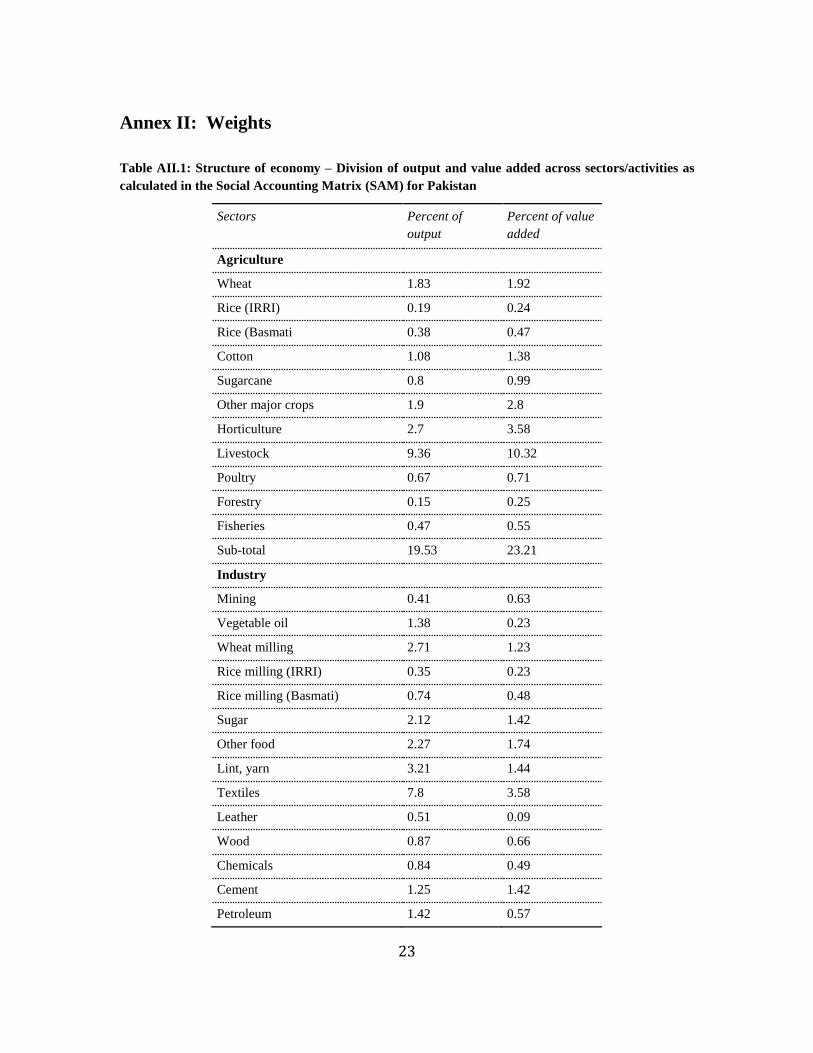
Annex II: Weights

Table AII.1: Structure of economy – Division of output and value added across sectors/activities as

calculated in the Social Accounting Matrix (SAM) for Pakistan

Sectors Percent of

output

Percent of value

added

Agriculture

Wheat 1.83 1.92

Rice (IRRI) 0.19 0.24

Rice (Basmati 0.38 0.47

Cotton 1.08 1.38

Sugarcane 0.8 0.99

Other major crops 1.9 2.8

Horticulture 2.7 3.58

Livestock 9.36 10.32

Poultry 0.67 0.71

Forestry 0.15 0.25

Fisheries 0.47 0.55

Sub-total 19.53 23.21

Industry

Mining 0.41 0.63

Vegetable oil 1.38 0.23

Wheat milling 2.71 1.23

Rice milling (IRRI) 0.35 0.23

Rice milling (Basmati) 0.74 0.48

Sugar 2.12 1.42

Other food 2.27 1.74

Lint, yarn 3.21 1.44

Textiles 7.8 3.58

Leather 0.51 0.09

Wood 0.87 0.66

Chemicals 0.84 0.49

Cement 1.25 1.42

Petroleum 1.42 0.57

24

Sectors Percent of

output

Percent of value

added

Other manufacturing 4.86 2.56

Energy 2.71 3.41

Sub-total 33.45 20.18

Services

Construction 3.66 3.16

Trade 8.79 15.28

Transport, communications 10.61 11.83

Housing 2.87 4.87

Private services 11.65 12.89

Public services 9.46 8.61

Sub-total 47.04 56.64

Total 100.02 100.03

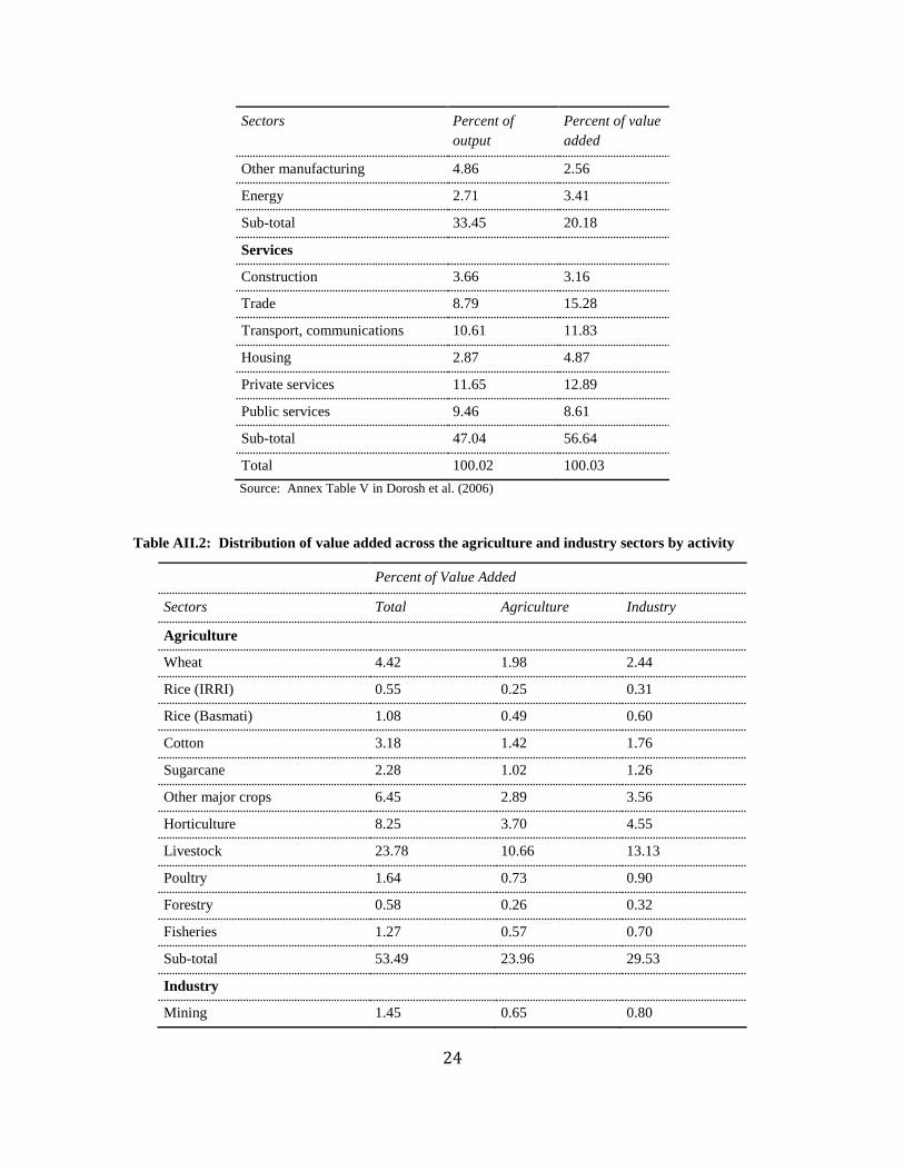
Source: Annex Table V in Dorosh et al. (2006)

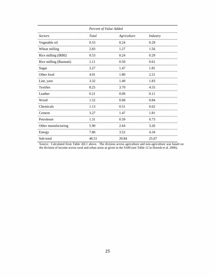
Table AII.2: Distribution of value added across the agriculture and industry sectors by activity

Percent of Value Added

Sectors Total Agriculture Industry

Agriculture

Wheat 4.42 1.98 2.44

Rice (IRRI) 0.55 0.25 0.31

Rice (Basmati) 1.08 0.49 0.60

Cotton 3.18 1.42 1.76

Sugarcane 2.28 1.02 1.26

Other major crops 6.45 2.89 3.56

Horticulture 8.25 3.70 4.55

Livestock 23.78 10.66 13.13

Poultry 1.64 0.73 0.90

Forestry 0.58 0.26 0.32

Fisheries 1.27 0.57 0.70

Sub-total 53.49 23.96 29.53

Industry

Mining 1.45 0.65 0.80

25

Percent of Value Added

Sectors Total Agriculture Industry

Vegetable oil 0.53 0.24 0.29

Wheat milling 2.83 1.27 1.56

Rice milling (IRRI) 0.53 0.24 0.29

Rice milling (Basmati) 1.11 0.50 0.61

Sugar 3.27 1.47 1.81

Other food 4.01 1.80 2.21

Lint, yarn 3.32 1.49 1.83

Textiles 8.25 3.70 4.55

Leather 0.21 0.09 0.11

Wood 1.52 0.68 0.84

Chemicals 1.13 0.51 0.62

Cement 3.27 1.47 1.81

Petroleum 1.31 0.59 0.73

Other manufacturing 5.90 2.64 3.26

Energy 7.86 3.52 4.34

Sub-total 46.51 20.84 25.67

Source: Calculated from Table AII.1 above. The division across agriculture and non-agriculture was based on

the division of income across rural and urban areas as given in the SAM (see Table 12 in Dorosh et al. 2006).

26

Annex III: The CGE Model for Pakistan

AIII.1 Model functioning

The Pakistan CGE model was developed by Cororaton and Orden (2008). The model

was calibrated to the 2001-02 Social Accounting Matrix (SAM) of Pakistan constructed

by Dorosh et al. (2006). The model has 34 production sectors spread over the following

categories: primary agriculture, lightly processed food, other manufacturing, services.

There are five input categories: 3 labor types (skilled labor, unskilled workers, and farm

labor), capital and land. There are 19 household categories, a government sector, a firm

sector and the rest of the world.

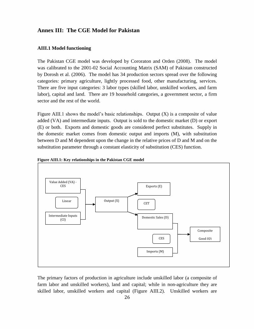
Figure AIII.1 shows the model’s basic relationships. Output (X) is a composite of value

added (VA) and intermediate inputs. Output is sold to the domestic market (D) or export

(E) or both. Exports and domestic goods are considered perfect substitutes. Supply in

the domestic market comes from domestic output and imports (M), with substitution

between D and M dependent upon the change in the relative prices of D and M and on the

substitution parameter through a constant elasticity of substitution (CES) function.

Figure AIII.1: Key relationships in the Pakistan CGE model

The primary factors of production in agriculture include unskilled labor (a composite of

farm labor and unskilled workers), land and capital; while in non-agriculture they are

skilled labor, unskilled workers and capital (Figure AIII.2). Unskilled workers are

Exports (E)

Value Added (VA) - CES

Intermediate Inputs (CI)

Output (X)

Domestic Sales (D)

Imports (M)

Composite

Good (Q)

CET

CES

Linear

27

assumed to be mobile across sectors because they are employed in agriculture and non-

agriculture sectors. Capital is fixed in each sector, with separate sectoral rates of return.

The use of land can shift among agricultural sub-sectors. Household income sources

derive from factors of production, transfers, foreign remittances, and dividends.

Household savings are a fixed proportion of disposable income and non-poor urban

households pay direct income tax to the government. Household demand is specified as a

linear expenditure system (LES).

The government sources its revenue from direct taxes on household and firm income,

indirect taxes on domestic and imported goods, tariffs and other receipts. Government

expenditures include consumption of goods and services, transfers and other payments.

Government income and balance are endogenous. Both government consumption and

foreign savings are fixed. The numéraire is a weighted index of the price of value added

where the weights are the sectoral value added shares at the base. The nominal exchange

rate is flexible. Furthermore, a weighted price of investment is introduced from which

total investment in real prices is derived. Total investment in real prices is held constant

by introducing an adjustment factor in the household savings function. Equilibrium in

the model is achieved when supply and demand of goods and services are in balance and

investment is equal to savings.

Figure AIII.2: Output determination in the Pakistan CGE model

Output (Linear)

Intermediate Inputs

Value Added (CES)

Skilled Labor Unskilled Labor (CES)

Capital Land (Agriculture only)

Workers Farm Labor

(Agriculture only)

28

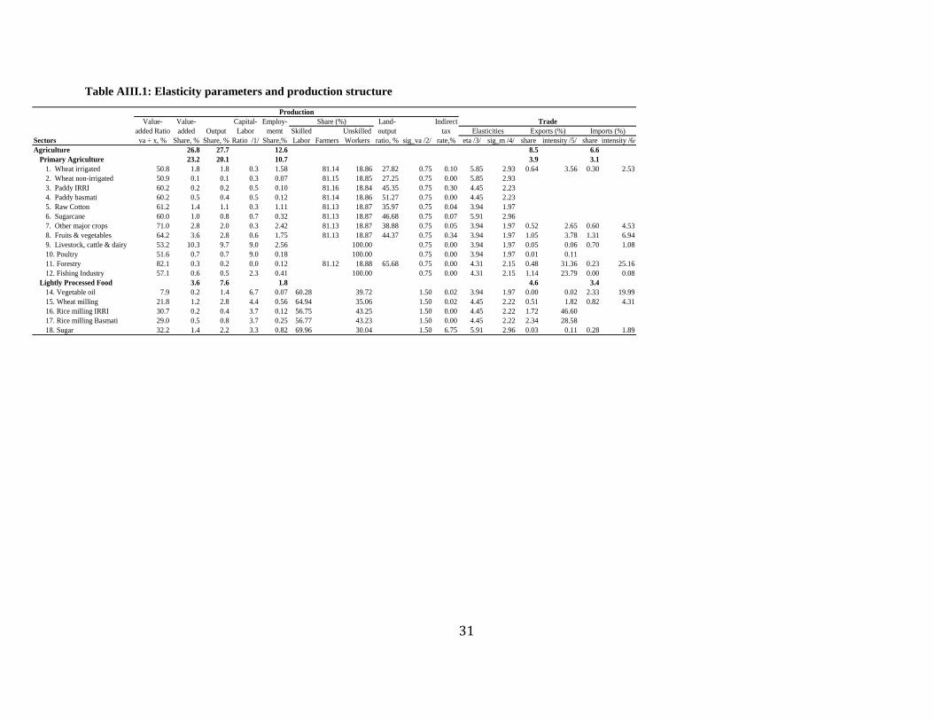
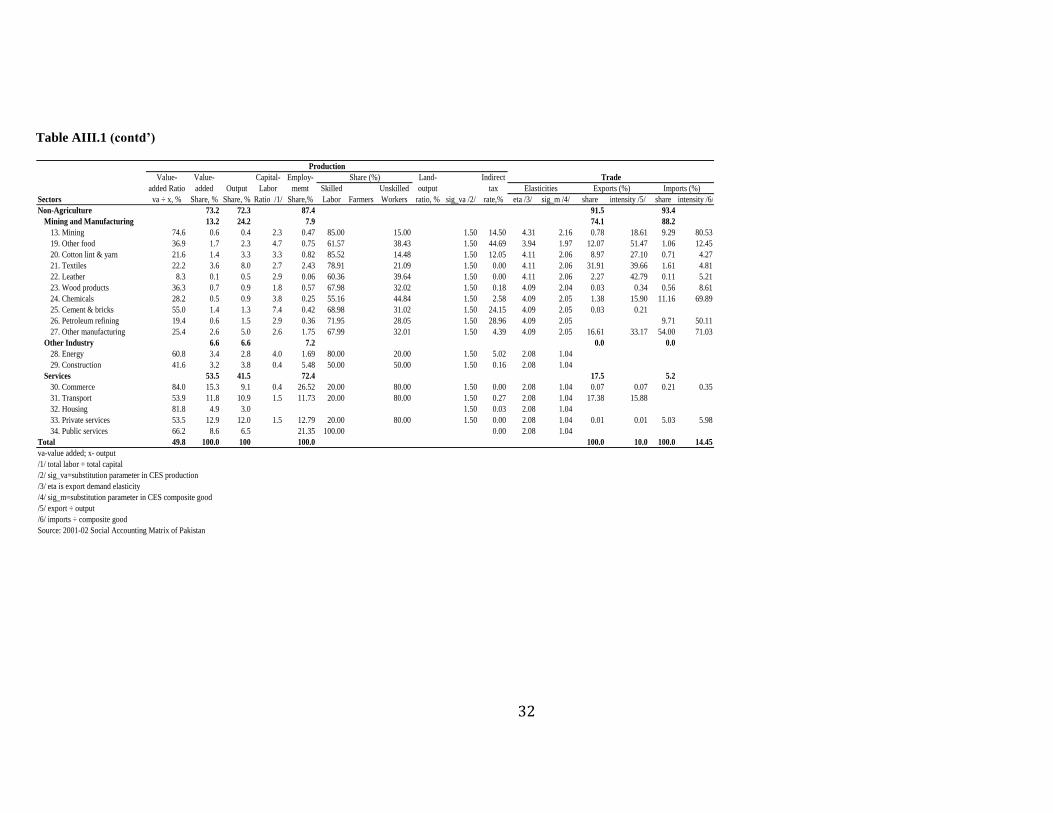
AIII.2 Economic structure in the SAM and key model parameters

Table AIII.1 shows the sectoral structure of production and trade in the model based on

the 2001-02 SAM; and Table AIII.2 shows the main household categories. Of the 34

sectors, 12 are primary agriculture. Five sectors under the heading of lightly processed

food are part of the broadly defined agricultural sector in this paper’s analysis. The non-

agricultural sectors include the mining industry, other food, manufacturing sectors,

energy, construction, and five service sectors. With these broad sectoral groupings,

agriculture produces 26.8 percent of total value added and 27.7 percent of total output. It

also provides 12.5 percent of total employment.

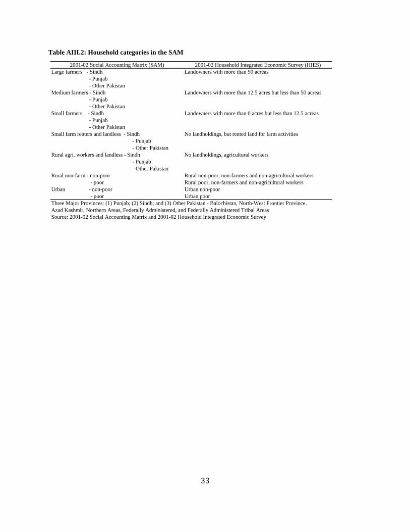
There are 19 household groups in the CGE model. The agricultural-based groups are

categorized by household location (Punjab, Sindh, and other Pakistan) and size of land

holdings (large, medium and small farms; landless and small-farm renters, and

agricultural workers without land). In addition, there are four national aggregates: rural

non-farm poor, and non-poor and urban poor and non-poor. Table AIII.2 shows the 19

households in the SAM and the corresponding characteristics of these 19 household

groups in the 2001-02 household income and expenditure survey (HIES).

The structure of consumption of each of these groups is given in Table AIII.3. A

composite sector ‘Livestock, cattle and dairy’ has the highest share in the consumption

basket, even though its share varies across household groups, from 14.4 percent in large

and medium farms in other Pakistan provinces to 24.9 percent in agricultural workers in

Punjab. The other major items in the consumption basket include private services (about

14 percent), transport (about 13 percent), wheat milling (from 4 percent among urban

non-poor to 11.7 percent among agricultural workers in other Pakistan provinces), textile

(from 4.9 percent in large and medium farms in other Pakistan provinces to 6.8 percent

among agricultural workers in Punjab and urban poor), other manufacturing (from 0.8

percent in agricultural workers in Sindh to 9.6 percent in large and medium farmers in

other Pakistan provinces), sugar (from 3.3 percent in urban non-poor to 9.6 percent in

agricultural workers in other Pakistan provinces), and fruits and vegetables (from 4.4

percent among large and medium farms in Punjab to 7.1 percent in agricultural workers

in other Pakistan provinces). Commodities with high foreign trade content will be

impacted significantly by changes in trade policies and world prices. This will have

varied effects across household groups because of differences in the consumption

structure.

The sectoral indirect tax structure is presented in Table AIII.1. The highest tax rate of

44.69 percent is on other food. But in Table AIII.3, the share of other food in the

consumption of households is only about 1 percent. Indirect taxes are also relatively high

29

on cement and bricks and petroleum refining, which generally account for less than 1

percent of household consumption directly but affect housing and transportation costs.

The tax rate on sugar is 6.75 percent and its share in the consumer basket ranges from 3.3

percent to 9.6 percent among the 19 household types. The tax rate on cotton lint and yarn

is 12.05 percent while the rate on textiles is zero. However, since cotton lint and yarn are

major inputs into textile production, an increase in the tax will increase the cost of

production of textiles. This will affect consumers since the share of textiles in the

consumption basket is about 5 percent.

Overall, the foreign trade sector in Pakistan is not very large relative to the domestic

sector. Of the total domestic output, only 10 percent goes to the export market. Of the

total goods and services available in the market, only 14.5 percent is imported. However,

there are large differences across sectors. For example, within agriculture, the sectors

with the highest export intensity ratio16

are milling of IRRI-type rice (46.6 percent),

forestry 31.4 percent, and fishing 23.8 percent. The export intensity ranges from 2.7

percent to 3.8 percent among ‘other major crops’, wheat irrigated, and fruits and

vegetables, while it is very small for the rest of the sectors. Within the non-agricultural

sectors, ‘other food’ has the highest ratio of 51.5 percent, leather 42.8 percent, textile

39.7 percent, and cotton lint and yarn 27.1 percent. The textile sector dominates exports.

In the SAM, textile exports have a 31.9 percent share of the total—dominant but less than

indicated in other trade account data. Cotton lint and yarn has a 9 percent export share,

while other food 12.1.

The highest import intensity ratio is for mining at 80.5 percent because of imports of

crude oil. The ratio for other manufacturing is 71 percent and chemicals 69.9 percent.

The import intensity ratio of petroleum is also high at 50.1 percent. Other manufacturing

accounts for 54 percent of overall imports, chemicals 11.2 percent, and mining and

petroleum refining each about 9 percent. Except for forestry (25.2 percent) and vegetable

oil (20 percent), import intensities for agricultural sectors are well under 10 percent.

Table AIII.1 also includes values of key elasticity parameters in the model: the import

substitution elasticity (sig_m) in the CES composite good function and the production

substitution elasticity (sig_va) in the CES value added production function.

The sources of household income in the model are labor income, capital income, income

from land, dividend income, and other income (Table AIII.4). There are three labor types

where labor income is derived: farmers, workers, and skilled workers. The other sources

16

Export intensity ratio is the sector’s export divided by its output, while import intensity ratio is the

sector’s imports divided by its total domestic supply.

30

of income are capital, land and other income, where other income is composed of foreign

remittances and dividend income.

The sources of income vary across groups. Farmers are heavily dependent on income

from farm labor, land and capital. Other rural households depend on income from

unskilled labor and capital. About three-fourths of income of urban poor comes from

unskilled workers. Urban non-poor households derive 44 percent of their income from

other income (composed largely of dividend income) and 33 percent from skilled labor

income.

Finally, Table AIII.4 also presents the structure of direct income tax. It is only the urban

non-poor household group that pays income tax, and even then a relatively low rate of 8.4

percent. The rest of the household groups do not pay any income tax at all.

31

Table AIII.1: Elasticity parameters and production structure

Value- Value- Capital- Employ- Land- Indirect

added Ratio added Output Labor memt Skilled Unskilled output tax

Sectors va ÷ x, % Share, % Share, % Ratio /1/ Share,% Labor Farmers Workers ratio, % sig_va /2/ rate,% eta /3/ sig_m /4/ share intensity /5/ share intensity /6/

Agriculture 26.8 27.7 12.6 8.5 6.6

Primary Agriculture 23.2 20.1 10.7 3.9 3.1

1. Wheat irrigated 50.8 1.8 1.8 0.3 1.58 81.14 18.86 27.82 0.75 0.10 5.85 2.93 0.64 3.56 0.30 2.53

2. Wheat non-irrigated 50.9 0.1 0.1 0.3 0.07 81.15 18.85 27.25 0.75 0.00 5.85 2.93

3. Paddy IRRI 60.2 0.2 0.2 0.5 0.10 81.16 18.84 45.35 0.75 0.30 4.45 2.23

4. Paddy basmati 60.2 0.5 0.4 0.5 0.12 81.14 18.86 51.27 0.75 0.00 4.45 2.23

5. Raw Cotton 61.2 1.4 1.1 0.3 1.11 81.13 18.87 35.97 0.75 0.04 3.94 1.97

6. Sugarcane 60.0 1.0 0.8 0.7 0.32 81.13 18.87 46.68 0.75 0.07 5.91 2.96

7. Other major crops 71.0 2.8 2.0 0.3 2.42 81.13 18.87 38.88 0.75 0.05 3.94 1.97 0.52 2.65 0.60 4.53

8. Fruits & vegetables 64.2 3.6 2.8 0.6 1.75 81.13 18.87 44.37 0.75 0.34 3.94 1.97 1.05 3.78 1.31 6.94

9. Livestock, cattle & dairy 53.2 10.3 9.7 9.0 2.56 100.00 0.75 0.00 3.94 1.97 0.05 0.06 0.70 1.08

10. Poultry 51.6 0.7 0.7 9.0 0.18 100.00 0.75 0.00 3.94 1.97 0.01 0.11

11. Forestry 82.1 0.3 0.2 0.0 0.12 81.12 18.88 65.68 0.75 0.00 4.31 2.15 0.48 31.36 0.23 25.16

12. Fishing Industry 57.1 0.6 0.5 2.3 0.41 100.00 0.75 0.00 4.31 2.15 1.14 23.79 0.00 0.08

Lightly Processed Food 3.6 7.6 1.8 4.6 3.4

14. Vegetable oil 7.9 0.2 1.4 6.7 0.07 60.28 39.72 1.50 0.02 3.94 1.97 0.00 0.02 2.33 19.99

15. Wheat milling 21.8 1.2 2.8 4.4 0.56 64.94 35.06 1.50 0.02 4.45 2.22 0.51 1.82 0.82 4.31

16. Rice milling IRRI 30.7 0.2 0.4 3.7 0.12 56.75 43.25 1.50 0.00 4.45 2.22 1.72 46.60

17. Rice milling Basmati 29.0 0.5 0.8 3.7 0.25 56.77 43.23 1.50 0.00 4.45 2.22 2.34 28.58

18. Sugar 32.2 1.4 2.2 3.3 0.82 69.96 30.04 1.50 6.75 5.91 2.96 0.03 0.11 0.28 1.89

Production

Share (%) Trade

Elasticities Exports (%) Imports (%)

32

Table AIII.1 (contd’)

Value- Value- Capital- Employ- Land- Indirect

added Ratio added Output Labor memt Skilled Unskilled output tax

Sectors va ÷ x, % Share, % Share, % Ratio /1/ Share,% Labor Farmers Workers ratio, % sig_va /2/ rate,% eta /3/ sig_m /4/ share intensity /5/ share intensity /6/

Non-Agriculture 73.2 72.3 87.4 91.5 93.4

Mining and Manufacturing 13.2 24.2 7.9 74.1 88.2

13. Mining 74.6 0.6 0.4 2.3 0.47 85.00 15.00 1.50 14.50 4.31 2.16 0.78 18.61 9.29 80.53

19. Other food 36.9 1.7 2.3 4.7 0.75 61.57 38.43 1.50 44.69 3.94 1.97 12.07 51.47 1.06 12.45

20. Cotton lint & yarn 21.6 1.4 3.3 3.3 0.82 85.52 14.48 1.50 12.05 4.11 2.06 8.97 27.10 0.71 4.27

21. Textiles 22.2 3.6 8.0 2.7 2.43 78.91 21.09 1.50 0.00 4.11 2.06 31.91 39.66 1.61 4.81

22. Leather 8.3 0.1 0.5 2.9 0.06 60.36 39.64 1.50 0.00 4.11 2.06 2.27 42.79 0.11 5.21

23. Wood products 36.3 0.7 0.9 1.8 0.57 67.98 32.02 1.50 0.18 4.09 2.04 0.03 0.34 0.56 8.61

24. Chemicals 28.2 0.5 0.9 3.8 0.25 55.16 44.84 1.50 2.58 4.09 2.05 1.38 15.90 11.16 69.89

25. Cement & bricks 55.0 1.4 1.3 7.4 0.42 68.98 31.02 1.50 24.15 4.09 2.05 0.03 0.21

26. Petroleum refining 19.4 0.6 1.5 2.9 0.36 71.95 28.05 1.50 28.96 4.09 2.05 9.71 50.11

27. Other manufacturing 25.4 2.6 5.0 2.6 1.75 67.99 32.01 1.50 4.39 4.09 2.05 16.61 33.17 54.00 71.03

Other Industry 6.6 6.6 7.2 0.0 0.0

28. Energy 60.8 3.4 2.8 4.0 1.69 80.00 20.00 1.50 5.02 2.08 1.04

29. Construction 41.6 3.2 3.8 0.4 5.48 50.00 50.00 1.50 0.16 2.08 1.04

Services 53.5 41.5 72.4 17.5 5.2

30. Commerce 84.0 15.3 9.1 0.4 26.52 20.00 80.00 1.50 0.00 2.08 1.04 0.07 0.07 0.21 0.35

31. Transport 53.9 11.8 10.9 1.5 11.73 20.00 80.00 1.50 0.27 2.08 1.04 17.38 15.88

32. Housing 81.8 4.9 3.0 1.50 0.03 2.08 1.04

33. Private services 53.5 12.9 12.0 1.5 12.79 20.00 80.00 1.50 0.00 2.08 1.04 0.01 0.01 5.03 5.98

34. Public services 66.2 8.6 6.5 21.35 100.00 0.00 2.08 1.04

Total 49.8 100.0 100 100.0 100.0 10.0 100.0 14.45

va-value added; x- output

/1/ total labor ÷ total capital

/2/ sig_va=substitution parameter in CES production

/3/ eta is export demand elasticity

/4/ sig_m=substitution parameter in CES composite good

/5/ export ÷ output

/6/ imports ÷ composite good

Source: 2001-02 Social Accounting Matrix of Pakistan

Production

Share (%) Trade

Elasticities Exports (%) Imports (%)

33

Table AIII.2: Household categories in the SAM

2001-02 Social Accounting Matrix (SAM) 2001-02 Household Integrated Economic Survey (HIES)

Large farmers - Sindh Landowners with more than 50 acreas

- Punjab

- Other Pakistan

Medium farmers - Sindh Landowners with more than 12.5 acres but less than 50 acreas

- Punjab

- Other Pakistan

Small farmers - Sindh Landowners with more than 0 acres but less than 12.5 acreas

- Punjab

- Other Pakistan

Small farm renters and landless - Sindh No landholdings, but rented land for farm activities

- Punjab

- Other Pakistan

Rural agri. workers and landless - Sindh No landholdings, agricultural workers

- Punjab

- Other Pakistan

Rural non-farm - non-poor Rural non-poor, non-farmers and non-agricultural workers

- poor Rural poor, non-farmers and non-agricultural workers

Urban - non-poor Urban non-poor

- poor Urban poor

Three Major Provinces: (1) Punjab; (2) Sindh; and (3) Other Pakistan - Balochistan, North-West Frontier Province,

Azad Kashmir, Northern Areas, Federally Administered, and Federally Administered Tribal Areas

Source: 2001-02 Social Accounting Matrix and 2001-02 Household Integrated Economic Survey

34

Table AIII.3: Consumption shares (%)

Commodities Sindh Punjab Others /a/ Sindh Punjab Others Sindh Punjab Others Sindh Punjab Others Sindh Punjab Others Non-Poor Poor Non-Poor Poor

Agriculture 45.9 40.1 38.8 45.8 40.1 38.8 49.1 47.9 48.6 52.3 47.6 47.1 53.9 51.9 50.8 43.9 49.8 38.4 47.3

Primary Agriculture 27.9 28.6 22.5 27.9 28.6 22.5 28.8 32.5 29.5 29.7 29.7 26.3 28.7 32.4 25.0 28.4 26.5 27.3 26.7

Other major crops 0.1 0.1 0.1 0.1 0.1 0.1 0.1 0.1 0.2 0.2 0.1 0.2 0.2 0.1 0.3 0.2 0.2 0.2 0.2

Fruits and vegetables 4.8 4.4 5.7 4.8 4.4 5.7 5.6 5.2 6.1 6.6 6.2 7.0 6.0 6.5 7.1 6.0 6.7 6.2 6.9

Livestock, cattle and dairy 19.9 22.8 14.4 19.9 22.8 14.4 19.5 26.1 21.6 19.3 22.3 17.5 20.7 24.9 15.9 19.9 17.9 18.3 18.0

Poultry 1.1 1.2 1.7 1.1 1.2 1.7 1.1 1.0 1.4 1.0 1.0 1.4 0.7 0.9 1.5 1.4 1.0 1.7 1.1

Forestry 0.0 0.1 0.0 0.0 0.1 0.0 0.0 0.1 0.1 0.0 0.0 0.1 0.0 0.0 0.0 0.1 0.0 0.0 0.0

Fishing Industry 1.9 0.0 0.5 1.9 0.0 0.5 2.5 0.0 0.1 2.7 0.0 0.2 1.2 - 0.3 0.9 0.7 0.8 0.6

Lightly Processed Food 18.0 11.5 16.3 18.0 11.5 16.3 20.2 15.5 19.0 22.6 17.9 20.8 25.2 19.6 25.8 15.5 23.3 11.1 20.6

Vegetable oil 2.9 2.8 2.7 2.9 2.8 2.7 3.3 3.3 3.3 3.4 3.6 3.4 3.2 3.4 3.8 3.2 3.9 2.7 3.8

Wheat milling 6.9 4.4 7.5 6.9 4.4 7.5 6.6 6.4 7.4 8.2 7.7 8.3 10.9 9.1 11.7 6.0 10.3 4.0 9.1

Rice milling IRRI 0.7 0.2 0.2 0.7 0.2 0.2 1.2 0.2 0.2 1.1 0.2 0.2 0.6 0.3 0.1 0.3 0.5 0.2 0.4

Rice milling Basmati 2.5 0.6 0.7 2.5 0.6 0.7 4.2 0.8 0.8 4.0 0.8 0.7 2.3 1.0 0.5 1.1 1.7 0.9 1.5

Sugar 5.0 3.6 5.3 5.0 3.6 5.3 4.9 4.8 7.3 5.9 5.5 8.2 8.2 5.8 9.6 5.0 7.0 3.3 5.8

Non-Agriculture 54.1 59.9 61.2 54.2 59.9 61.2 50.9 52.1 51.4 47.7 52.4 52.9 46.1 48.1 49.2 56.1 50.2 61.6 52.7

Mining and Manufacturing 17.2 22.4 22.9 17.2 22.4 23.0 14.2 15.4 14.2 10.9 15.4 15.6 9.8 11.8 12.2 18.0 13.3 20.3 14.3

Mining 0.0 0.0 0.0 0.0 0.0 0.0 0.0 0.0 0.0 0.0 0.0 0.0 0.0 0.0 0.0 0.0 0.0 0.0 0.0

Other food 1.2 0.9 1.3 1.2 0.9 1.3 1.2 1.0 1.9 1.6 1.2 1.9 1.5 1.0 2.2 1.6 1.5 1.9 1.6

Cotton lint and yarn - - - - - - - - - - - - - - - - - - -

Textiles 5.5 6.6 4.9 5.5 6.6 4.9 6.0 6.2 5.3 6.7 6.5 5.3 6.1 6.8 5.1 5.8 6.6 5.8 6.8

Leather 0.2 0.4 0.3 0.2 0.4 0.3 0.2 0.3 0.3 0.3 0.3 0.3 0.2 0.4 0.3 0.3 0.3 0.3 0.4

Wood products - - - - - - - - - - - - - - - - - - -

Chemicals 3.0 4.3 4.9 3.0 4.3 4.9 1.9 2.2 1.8 0.5 2.1 2.3 0.4 0.9 1.2 2.9 1.3 3.5 1.4

Cement_bricks 0.9 1.2 1.4 0.9 1.2 1.4 0.5 0.6 0.5 0.1 0.6 0.6 0.1 0.3 0.3 0.8 0.4 1.0 0.4

Petroleum refining 0.5 0.5 0.6 0.5 0.5 0.6 0.5 0.6 0.8 0.7 0.7 0.8 0.6 0.6 0.8 0.8 0.8 0.9 1.0

Other manufacturing 5.8 8.4 9.6 5.8 8.4 9.6 3.7 4.4 3.5 1.0 4.0 4.4 0.8 1.8 2.2 5.7 2.5 6.9 2.7

Other Industry 0.6 0.7 0.7 0.6 0.7 0.7 0.6 0.7 1.0 0.9 0.8 0.9 0.8 0.7 1.0 0.9 1.0 1.1 1.2

Energy 0.6 0.7 0.7 0.6 0.7 0.7 0.6 0.7 1.0 0.9 0.8 0.9 0.8 0.7 1.0 0.9 1.0 1.1 1.2

Construction - - - - - - - - - - - - - - - - - - -

Services 36.3 36.9 37.5 36.3 36.9 37.5 36.1 36.0 36.3 35.9 36.1 36.4 35.5 35.5 36.0 37.2 35.9 40.2 37.2

Commerce 3.5 3.5 3.5 3.5 3.5 3.5 3.5 3.5 3.5 3.4 3.5 3.5 3.4 3.4 3.4 3.5 3.4 3.4 3.4

Transport 13.5 13.6 13.6 13.5 13.6 13.6 13.3 13.4 13.3 13.1 13.3 13.3 13.1 13.1 13.2 13.4 13.2 13.1 13.0

Housing 1.4 1.6 2.4 1.4 1.6 2.4 1.5 1.3 1.8 1.9 1.7 1.8 1.6 1.5 1.8 2.5 1.7 6.3 3.5

Private services 14.5 14.7 14.6 14.5 14.7 14.6 14.4 14.4 14.4 14.2 14.4 14.4 14.1 14.2 14.3 14.4 14.3 14.1 14.1

Public services 3.4 3.4 3.4 3.4 3.4 3.4 3.4 3.4 3.4 3.3 3.3 3.4 3.3 3.3 3.3 3.4 3.3 3.3 3.3

Total 100 100 100 100 100 100 100 100 100 100 100 100 100 100 100 100 100 100 100

/a/ Others - Balochistan, North-West Frontier Province, Azad Kashmir, Northern Areas, Federally Administered, and Federally Administered Tribal Areas

Source: 2001-2002 Social Accounting Matrix of Pakistan

Other Rural UrbanLarge Farmers Medium Farmers Small Farmers Small Farm Renters Agri. Workers

35

Table AIII.4: Sources of household income and income tax

Total Per Capita Direct

Households mil Rs '000 Rs '000 % dist. Farmers Workers Skilled K Land Others tax, %

Large farmers - Sindh 19,079 112.9 169 0.12 13.2 0.3 - 31.4 49.8 5.3 -

- Punjab 64,116 173.7 369 0.25 8.6 0.5 - 43.3 42.2 5.4 -

- Other Pakistan /a/ 10,755 152.9 70 0.05 9.8 0.2 - 52.4 32.3 5.4 -

Medium farmers - Sindh 44,625 30.4 1,466 1.00 14.5 3.1 - 39.6 37.4 5.3 -

- Punjab 145,995 48.4 3,014 2.07 10.8 4.3 - 52.3 27.2 5.4 -

- Other Pakistan 35,572 34.2 1,040 0.71 14.9 2.9 - 38.2 38.4 5.5 -

Small farmers - Sindh 57,648 14.9 3,873 2.65 6.8 9.0 - 57.9 20.4 5.8 -

- Punjab 318,888 18.1 17,605 12.06 7.9 14.2 - 51.8 20.3 5.8 -

- Other Pakistan 124,985 11.9 10,493 7.19 6.0 11.6 - 63.6 12.5 6.2 -

Small farm renters and landless - Sindh 43,672 7.7 5,682 3.89 11.6 18.7 - 48.5 15.6 5.7 -

- Punjab 45,963 10.7 4,307 2.95 9.0 20.5 - 48.7 16.1 5.8 -

- Other Pakistan 14,970 8.2 1,818 1.25 10.1 14.5 - 55.0 14.7 5.7 -

Rural agri. workers and landless - Sindh 20,782 6.4 3,241 2.22 - 51.0 - 42.8 - 6.2 -

- Punjab 68,172 12.0 5,693 3.90 - 49.3 - 45.2 - 5.5 -

- Other Pakistan 9,513 14.6 653 0.45 - 18.7 - 76.0 - 5.4 -

Rural non-farm - non-poor 400,771 19.8 20,233 13.86 - 43.0 - 49.9 - 7.2 -

- poor 134,398 5.5 24,525 16.80 - 29.7 - 63.4 - 6.9 -

Urban - non-poor 1,744,119 58.5 29,829 20.44 - 11.9 33.3 10.6 - 44.2 8.4

- poor 181,413 15.3 11,880 8.14 - 76.2 - 18.0 - 5.8 -

/a/ Other Pakistan - Balochistan, North-West Frontier Province, Azad Kashmir, Northern Areas, Federally Administered, and Federally Administered Tribal Areas

Source: 2001-2002 Social Accounting Matrix of Pakistan

2001-02 Income

2001-02 Pop.

Income Sources, %

Labor