working set selection using second order information …cjlin/papers/quadworkset.pdf · working set...

Journal of Machine Learning Research 6 (2005) 1889–1918 Submitted 04/05; Revised 10/05; Published 11/05

Working Set Selection Using Second Order Information

for Training Support Vector Machines

Rong-En Fan [email protected]

Pai-Hsuen Chen [email protected]

Chih-Jen Lin [email protected]

Department of Computer Science, National Taiwan University

Taipei 106, Taiwan

Editor: Thorsten Joachims

Abstract

Working set selection is an important step in decomposition methods for training supportvector machines (SVMs). This paper develops a new technique for working set selection inSMO-type decomposition methods. It uses second order information to achieve fast con-vergence. Theoretical properties such as linear convergence are established. Experimentsdemonstrate that the proposed method is faster than existing selection methods using firstorder information.

Keywords: support vector machines, decomposition methods, sequential minimal opti-mization, working set selection

1. Introduction

Support vector machines (SVMs) (Boser et al., 1992; Cortes and Vapnik, 1995) are a usefulclassification method. Given instances xi, i = 1, . . . , l with labels yi ∈ {1,−1}, the maintask in training SVMs is to solve the following quadratic optimization problem:

minα

f(α) =1

2αT Qα − eT α

subject to 0 ≤ αi ≤ C, i = 1, . . . , l, (1)

yT α = 0,

where e is the vector of all ones, C is the upper bound of all variables, Q is an l by lsymmetric matrix with Qij = yiyjK(xi,xj), and K(xi,xj) is the kernel function.

The matrix Q is usually fully dense and may be too large to be stored. Decompositionmethods are designed to handle such difficulties (e.g., Osuna et al., 1997; Joachims, 1998;Platt, 1998; Chang and Lin, 2001). Unlike most optimization methods which update thewhole vector α in each step of an iterative process, the decomposition method modifies onlya subset of α per iteration. This subset, denoted as the working set B, leads to a smallsub-problem to be minimized in each iteration. An extreme case is the Sequential MinimalOptimization (SMO) (Platt, 1998), which restricts B to have only two elements. Then ineach iteration one does not require any optimization software in order to solve a simpletwo-variable problem. This method is sketched in the following:

c©2005 Rong-En Fan, Pai-Hsuen Chen, and Chih-Jen Lin.

Fan, Chen, and Lin

Algorithm 1 (SMO-type decomposition method)1. Find α1 as the initial feasible solution. Set k = 1.

2. If αk is an optimal solution of (1), stop. Otherwise, find a two-element working setB = {i, j} ⊂ {1, . . . , l}. Define N ≡ {1, . . . , l}\B and αk

B and αkN to be sub-vectors

of αk corresponding to B and N , respectively.

3. Solve the following sub-problem with the variable αB:

minαB

1

2

[

αTB (αk

N )T]

[

QBB QBN

QNB QNN

] [

αB

αkN

]

−[

eTB eT

N

]

[

αB

αkN

]

=1

2αT

BQBBαB + (−eB + QBNαkN )T αB + constant

=1

2

[

αi αj

]

[

Qii Qij

Qij Qjj

] [

αi

αj

]

+ (−eB + QBNαkN )T

[

αi

αj

]

+ constant

subject to 0 ≤ αi, αj ≤ C, (2)

yiαi + yjαj = −yTNαk

N ,

where[

QBB QBN

QNB QNN

]

is a permutation of the matrix Q.

4. Set αk+1B to be the optimal solution of (2) and αk+1

N ≡ αkN . Set k ← k + 1 and goto

Step 2.

Note that the set B changes from one iteration to another, but to simplify the notation, wejust use B instead of Bk.

Since only few components are updated per iteration, for difficult problems, the decom-position method suffers from slow convergences. Better methods of working set selectioncould reduce the number of iterations and hence are an important research issue. Existingmethods mainly rely on the violation of the optimality condition, which also corresponds tofirst order (i.e., gradient) information of the objective function. Past optimization researchindicates that using second order information generally leads to faster convergence. Now(1) is a quadratic programming problem, so second order information directly relates to thedecrease of the objective function. There are several attempts (e.g., Lai et al., 2003a,b) tofind working sets based on the reduction of the objective value, but these selection methodsare only heuristics without convergence proofs. Moreover, as such techniques cost morethan existing ones, fewer iterations may not lead to shorter training time. This paper de-velops a simple working set selection using second order information. It can be extendedfor indefinite kernel matrices. Experiments demonstrate that the training time is shorterthan existing implementations.

This paper is organized as follows. In Section 2, we discuss existing methods of workingset selection and propose a new strategy. Theoretical properties of using the new selectiontechnique are in Section 3. In Section 4 we extend the proposed selection method to otherSVM formulas such as ν-SVM. A detailed experiment is in Section 5. We then in Section6 discuss and compare some variants of the proposed selection method. Finally, Section 7concludes this research work. A pseudo code of the proposed method is in the Appendix.

1890

Working Set Selection for Training SVMs

2. Existing and New Working Set Selections

In this section, we discuss existing methods of working set selection and then propose a newapproach.

2.1 Existing Selections

Currently a popular way to select the working set B is via the “maximal violating pair:”

WSS 1 (Working set selection via the “maximal violating pair”)1. Select

i ∈ arg maxt

{−yt∇f(αk)t | t ∈ Iup(αk)},

j ∈ arg mint{−yt∇f(αk)t | t ∈ Ilow(αk)},

where

Iup(α) ≡ {t | αt < C, yt = 1 or αt > 0, yt = −1}, and

Ilow(α) ≡ {t | αt < C, yt = −1 or αt > 0, yt = 1}.(3)

2. Return B = {i, j}.

This working set was first proposed in Keerthi et al. (2001) and is used in, for example,the software LIBSVM (Chang and Lin, 2001). WSS 1 can be derived through the Karush-Kuhn-Tucker (KKT) optimality condition of (1): A vector α is a stationary point of (1) ifand only if there is a number b and two nonnegative vectors λ and µ such that

∇f(α) + by = λ − µ,

λiαi = 0, µi(C − αi) = 0, λi ≥ 0, µi ≥ 0, i = 1, . . . , l,

where ∇f(α) ≡ Qα − e is the gradient of f(α). This condition can be rewritten as

∇f(α)i + byi ≥ 0 if αi < C, (4)

∇f(α)i + byi ≤ 0 if αi > 0. (5)

Since yi = ±1, by defining Iup(α) and Ilow(α) as in (3), and rewriting (4)-(5) to

−yi∇f(α)i ≤ b, ∀i ∈ Iup(α), and

−yi∇f(α)i ≥ b, ∀i ∈ Ilow(α),

a feasible α is a stationary point of (1) if and only if

m(α) ≤ M(α), (6)

wherem(α) ≡ max

i∈Iup(α)−yi∇f(α)i, and M(α) ≡ min

i∈Ilow(α)−yi∇f(α)i.

Note that m(α) and M(α) are well defined except a rare situation where all yi = 1 (or−1). In this case the zero vector is the only feasible solution of (1), so the decompositionmethod stops at the first iteration.

Following Keerthi et al. (2001), we define a “violating pair” of the condition (6).

1891

Fan, Chen, and Lin

Definition 1 (Violating pair) If i ∈ Iup(α), j ∈ Ilow(α), and −yi∇f(α)i > −yj∇f(α)j,then {i, j} is a “violating pair.”

From (6), indices {i, j} which most violate the optimality condition are a natural choice ofthe working set. They are called a “maximal violating pair” in WSS 1. It is known thatviolating pairs are important in the working set selection:

Theorem 2 (Hush and Scovel, 2003) Assume Q is positive semi-definite. SMO-typemethods have the strict decrease of the function value (i.e., f(αk+1) < f(αk),∀k) if andonly if B is a violating pair.

Interestingly, the maximal violating pair is related to first order approximation of f(α).As explained below, {i, j} selected via WSS 1 satisfies

{i, j} = arg minB:|B|=2

Sub(B), (7)

where

Sub(B) ≡ mindB

∇f(αk)TBdB (8a)

subject to yTBdB = 0,

dt ≥ 0, if αkt = 0, t ∈ B, (8b)

dt ≤ 0, if αkt = C, t ∈ B, (8c)

−1 ≤ dt ≤ 1, t ∈ B. (8d)

Problem (7) was first considered in Joachims (1998). By defining dT ≡ [dTB,0T

N ], theobjective function (8a) comes from minimizing first order approximation of f(αk + d):

f(αk + d) ≈ f(αk) + ∇f(αk)Td

= f(αk) + ∇f(αk)TBdB.

The constraint yTBdB = 0 is from yT (αk +d) = 0 and yT αk = 0. The condition 0 ≤ αt ≤ C

leads to inequalities (8b) and (8c). As (8a) is a linear function, the inequalities −1 ≤ dt ≤1, t ∈ B avoid that the objective value goes to −∞.

A first look at (7) indicates that we may have to check all(

l2

)

B’s in order to find anoptimal set. Instead, WSS 1 efficiently solves (7) in O(l) steps. This result is discussed inLin (2001a, Section II), where more general settings (|B| is any even integer) are considered.The proof for |B| = 2 is easy, so we give it in Appendix A for completeness.

The convergence of the decomposition method using WSS 1 is proved in Lin (2001a,2002).

2.2 A New Working Set Selection

Instead of using first order approximation, we may consider more accurate second orderinformation. As f is a quadratic,

f(αk + d) − f(αk) = ∇f(αk)Td +1

2dT∇2f(αk)d

= ∇f(αk)TBdB +

1

2dT

B∇2f(αk)BBdB (9)

1892


is exactly the reduction of the objective value. Thus, by replacing the objective function of(8) with (9), a selection method using second order information is

minB:|B|=2

Sub(B), (10)

where

Sub(B) ≡ mindB

1

2dT

B∇2f(αk)BBdB + ∇f(αk)T

BdB (11a)

subject to yTBdB = 0, (11b)

dt ≥ 0, if αkt = 0, t ∈ B, (11c)

dt ≤ 0, if αkt = C, t ∈ B. (11d)

Note that inequality constraints −1 ≤ dt ≤ 1, t ∈ B in (8) are removed, as later we willsee that the optimal value of (11) does not go to −∞. Though one expects (11) is betterthan (8), minB:|B|=2 Sub(B) in (10) becomes a challenging task. Unlike (7)-(8), which canbe efficiently solved by WSS 1, for (10) and (11) there is no available way to avoid checkingall

(

l2

)

B’s. Note that except the working set selection, the main task per decompositioniteration is on calculating the two kernel columns Qti and Qtj , t = 1, . . . , l. This requiresO(l) operations and is needed only if Q is not stored. Therefore, each iteration can becomel times more expensive if an O(l2) working set selection is used. Moreover, from simpleexperiments we know that the number of iterations is, however, not decreased l times.Therefore, an O(l2) working set selection is impractical.

A viable implementation of using second order information is thus to heuristically checkseveral B’s only. We propose the following new selection:

WSS 2 (Working set selection using second order information)1. Select

i ∈ arg maxt

{−yt∇f(αk)t | t ∈ Iup(αk)}.

2. Consider Sub(B) defined in (11) and select

j ∈ arg mint{Sub({i, t}) | t ∈ Ilow(αk),−yt∇f(αk)t < −yi∇f(αk)i}. (12)


By using the same i as in WSS 1, we check only O(l) possible B’s to decide j. Alternatively,one may choose j ∈ arg M(αk) and search for i by a way similar to (12)1. In fact, such aselection is the same as swapping labels y first and then applying WSS 2, so the performanceshould not differ much. It is certainly possible to consider other heuristics, and the mainconcern is how good they are if compared to the one by fully checking all

(

l2

)

sets. InSection 7 we will address this issue. Experiments indicate that a full check does not reduceiterations of using WSS 2 much. Thus WSS 2 is already a very good way of using secondorder information.

1. To simplify the notations, we denote arg M(α) as arg mint∈Ilow(α) −yt∇f(α)t and arg m(α) asarg maxt∈Iup(α) −yt∇f(α)t, respectively.

1893

Fan, Chen, and Lin

Despite the above issue of how to effectively use second order information, the realchallenge is whether the new WSS 2 can cause shorter training time than WSS 1. Now thetwo selection methods differ only in selecting j, so we can also consider WSS 2 as a directattempt to improve WSS 1. The following theorem shows that one could efficiently solve(11), so the working set selection WSS 2 does not cost a lot more than WSS 1.

Theorem 3 If B = {i, j} is a violating pair and Kii + Kjj − 2Kij > 0, then (11) has theoptimal objective value

−(−yi∇f(αk)i + yj∇f(αk)j)

2

2(Kii + Kjj − 2Kij).

Proof Define di ≡ yidi and dj ≡ yjdj . From yTBdB = 0, we have di = −dj and

1

2

[

di dj

]

[

Qii Qij

Qij Qjj

] [

di

dj

]

+[

∇f(αk)i ∇f(αk)j

]

[

di

dj

]

=1

2(Kii + Kjj − 2Kij)d

2j + (−yi∇f(αk)i + yj∇f(αk)j)dj . (13)

Since Kii + Kjj − 2Kij > 0 and B is a violating pair, we can define

aij ≡ Kii + Kjj − 2Kij > 0 and bij ≡ −yi∇f(αk)i + yj∇f(αk)j > 0. (14)

Then (13) has the minimum at

dj = −di = −bij

aij< 0, (15)

and

the objective function (11a) = −b2ij

2aij.

Moreover, we can show that di and dj (di and dj) indeed satisfy (11c)-(11d). If

j ∈ Ilow(αk), αkj = 0 implies yj = −1 and hence dj = yj dj > 0, a condition required

by (11c). Other cases are similar. Thus di and di defined in (15) are optimal for (11).

Note that if K is positive definite, then for any i 6= j, Kii + Kjj − 2Kij > 0. UsingTheorem 3, (12) in WSS 2 is reduced to a very simple form:

j ∈ arg mint

{

−b2it

ait| t ∈ Ilow(αk),−yt∇f(αk)t < −yi∇f(αk)i

}

,

where ait and bit are defined in (14). If K is not positive definite, the leading coefficient aij

of (13) may be non-positive. This situation will be addressed in the next sub-section.Note that (8) and (11) are used only for selecting the working set, so they do not have

to maintain the feasibility 0 ≤ αki + di ≤ C,∀i ∈ B. On the contrary, feasibility must

hold for the sub-problem (2) used to obtain αk+1 after B is determined. There are someearlier attempts to use second order information for selecting working sets (e.g., Lai et al.,2003a,b), but they always check the feasibility. Then solving sub-problems during the

1894


selection procedure is more complicated than solving the sub-problem (11). Besides, theseearlier approaches do not provide any convergence analysis. In Section 6 we will investigatethe issue of maintaining feasibility in the selection procedure, and explain why using (11)is better.

2.3 Non-Positive Definite Kernel Matrices

Theorem 3 does not hold if Kii + Kjj − 2Kij ≤ 0. For the linear kernel, sometimes K isonly positive semi-definite, so it is possible that Kii + Kjj − 2Kij = 0. Moreover, someexisting kernel functions (e.g., sigmoid kernel) are not the inner product of two vectors, soK is even not positive semi-definite. Then Kii + Kjj − 2Kij < 0 may occur and (13) is aconcave objective function.

Once B is decided, the same difficulty occurs for the sub-problem (2) to obtain αk+1.Note that (2) differs from (11) only in constraints; (2) strictly requires the feasibility 0 ≤ αi+di ≤ C,∀t ∈ B. Therefore, (2) also has a concave objective function if Kii +Kjj −2Kij < 0.In this situation, (2) may possess multiple local minima. Moreover, there are difficultiesin proving the convergence of the decomposition methods (Palagi and Sciandrone, 2005;Chen et al., 2006). Thus, Chen et al. (2006) proposed adding an additional term to (2)’sobjective function if aij ≡ Kii + Kjj − 2Kij ≤ 0:

minαi,αj

1

2

[

αi αj

]

[

Qii Qij

Qij Qjj

] [

αi

αj

]

+ (−eB + QBNαkN )T

[

αi

αj

]

+

τ − aij

4((αi − αk

i )2 + (αj − αk

j )2)

subject to 0 ≤ αi, αj ≤ C, (16)

yiαi + yjαj = −yTNαk

N ,

where τ is a small positive number. By defining di ≡ yi(αi − αki ) and dj ≡ yj(αj − αk

j ),(16)’s objective function, in a form similar to (13), is

1

2τ d2

j + bij dj , (17)

where bij is defined as in (14). The new objective function is thus strictly convex. If {i, j}

is a violating pair, then a careful check shows that there is dj < 0 which leads to a negativevalue in (17) and maintains the feasibility of (16). Therefore, we can find αk+1 6= αk

satisfying f(αk+1) < f(αk). More details are in Chen et al. (2006).For selecting the working set, we consider a similar modification: If B = {i, j} and aij

is defined as in (14), then (11) is modified to:

Sub(B) ≡ mindB

1

2dT


BdB +τ − aij

4(d2

i + d2j )

subject to constraints of (11).

(18)

Note that (18) differs from (16) only in constraints. In (18) we do not maintain the feasibilityof αk

t + dt, t ∈ B. We are allowed to do so because (18) is used only for identifying theworking set B.

1895

Fan, Chen, and Lin

By reformulating (18) to (17) and following the same argument in Theorem 3, theoptimal objective value of (18) is

−b2ij

2τ.

Therefore, a generalized working set selection is as the following:

WSS 3(Working set selection using second order information: any symmetric K)

1. Define ats and bts as in (14), and

ats ≡

{

ats if ats > 0,τ otherwise.

(19)

Select

i ∈ arg maxt

{−yt∇f(αk)t | t ∈ Iup(αk)},

j ∈ arg mint

{

−b2it

ait| t ∈ Ilow(αk),−yt∇f(αk)t < −yi∇f(αk)i

}

. (20)


In summary, an SMO-type decomposition method using WSS 3 for the working set selectionis:

Algorithm 2 (An SMO-type decomposition method using WSS 3)1. Find α1 as the initial feasible solution. Set k = 1.

2. If αk is a stationary point of (1), stop. Otherwise, find a working set B = {i, j} byWSS 3.

3. Let aij be defined as in (14). If aij > 0, solve the sub-problem (2). Otherwise, solve(16). Set αk+1

B to be the optimal point of the sub-problem.

4. Set αk+1N ≡ αk

N . Set k ← k + 1 and goto Step 2.

In the next section we study theoretical properties of using WSS 3.

3. Theoretical Properties

To obtain theoretical properties of using WSS 3, we consider the work (Chen et al., 2006),which gives a general study of SMO-type decomposition methods. It considers Algorithm2 but replaces WSS 3 with a general working set selection2:

WSS 4 (A general working set selection discussed in Chen et al., 2006)1. Consider a fixed 0 < σ ≤ 1 for all iterations.

2. In fact, Chen et al. (2006) consider an even more general framework for selecting working sets, but foreasy description, we discuss WSS 4 here.

1896


2. Select any i ∈ Iup(αk), j ∈ Ilow(αk) satisfying

− yi∇f(αk)i + yj∇f(αk)j ≥ σ(m(αk) − M(αk)) > 0. (21)


Clearly (21) ensures the quality of the selected pair by linking it to the maximal violatingpair. It is easy to see that WSS 3 is a special case of WSS 4: Assume B = {i, j} is the setreturned from WSS 3 and j ∈ arg M(αk). Since WSS 3 selects i ∈ arg m(αk), with aij > 0and aij > 0, (20) in WSS 3 implies

−(−yi∇f(αk)i + yj∇f(αk)j)2

aij≤

−(m(αk) − M(αk))2

aij

.

Thus,

−yi∇f(αk)i + yj∇f(αk)j ≥

√

mint,s at,s

maxt,s at,s(m(αk) − M(αk)),

an inequality satisfying (21) for σ =√

mint,s at,s/ maxt,s at,s.Therefore, all theoretical properties proved in Chen et al. (2006) hold here. They are

listed below.It is known that the decomposition method may not converge to an optimal solution if

using improper methods of working set selection. We thus must prove that the proposedselection leads to the convergence.

Theorem 4 (Asymptotic convergence (Chen et al., 2006, Theorem 3 and Corol-lary 1))

Let {αk} be the infinite sequence generated by the SMO-type method Algorithm 2. Thenany limit point of {αk} is a stationary point of (1). Moreover, if Q is positive definite,{αk} globally converges to the unique minimum of (1).

As the decomposition method only asymptotically approaches an optimum, in practice,it is terminated after satisfying a stopping condition. For example, we can pre-specify asmall tolerance ǫ > 0 and check if the maximal violation is small enough:

m(αk) − M(αk) ≤ ǫ. (22)

Alternatively, one may check if the selected working set {i, j} satisfies

− yi∇f(αk)i + yj∇f(αk)j ≤ ǫ, (23)

because (21) implies m(αk)−M(αk) ≤ ǫ/σ. These are reasonable stopping criteria due totheir closeness to the optimality condition (6). To avoid an infinite loop, we must have thatunder any ǫ > 0, Algorithm 2 stops in a finite number of iterations. The finite terminationof using (22) or (23) as the stopping condition is implied by (26) of Theorem 5 stated below.

Shrinking and caching (Joachims, 1998) are two effective techniques to make the decom-position method faster. The former removes some bounded components during iterations,so smaller reduced problems are considered. The latter allocates some memory space (calledcache) to store recently used Qij , and may significantly reduce the number of kernel evalu-ations. The following theorem explains why these two techniques are useful in practice:

1897

Fan, Chen, and Lin

Theorem 5 (Finite termination and explanation of caching and shrinking tech-niques (Chen et al., 2006, Theorems 4 and 6))

Assume Q is positive semi-definite.

1. The following set is independent of any optimal solution α:

I ≡ {i | −yi∇f(α)i > M(α) or − yi∇f(α)i < m(α)}. (24)

Problem (1) has unique and bounded optimal solutions at αi, i ∈ I.

2. Assume Algorithm 2 generates an infinite sequence {αk}. There is k such that afterk ≥ k, every αk

i , i ∈ I has reached the unique and bounded optimal solution. It remainsthe same in all subsequent iterations and ∀k ≥ k:

i 6∈ {t | M(αk) ≤ −yt∇f(αk)t ≤ m(αk)}. (25)

3. If (1) has an optimal solution α satisfying m(α) < M(α), then α is the uniquesolution and Algorithm 2 reaches it in a finite number of iterations.

4. If {αk} is an infinite sequence, then the following two limits exist and are equal:

limk→∞

m(αk) = limk→∞

M(αk) = m(α) = M(α), (26)

where α is any optimal solution.

Finally, the following theorem shows that Algorithm 2 is linearly convergent under someassumptions:

Theorem 6 (Linear convergence (Chen et al., 2006, Theorem 8))Assume problem (1) satisfies

1. Q is positive definite. Therefore, (1) has a unique optimal solution α.

2. The nondegenency condition. That is, the optimal solution α satisfies that

∇f(α)i + byi = 0 if and only if 0 < αi < C, (27)

where b = m(α) = M(α) according to Theorem 5.

For the sequence {αk} generated by Algorithm 2, there are c < 1 and k such that for allk ≥ k,

f(αk+1) − f(α) ≤ c(f(αk) − f(α)).

This theorem indicates how fast the SMO-type method Algorithm 2 converges. For anyfixed problem (1) and a given tolerance ǫ, there is k such that within

k + O(log(1/ǫ))

iterations,|f(αk) − f(α)| ≤ ǫ.

Note that O(log(1/ǫ)) iterations are necessary for decomposition methods according to theanalysis in Lin (2001b)3. Hence the result of linear convergence here is already the bestworst case analysis.

3. Lin (2001b) gave a three-variable example and explained that the SMO-type method using WSS 1 islinearly convergent. A careful check shows that the same result holds for any method of working setselection.

1898


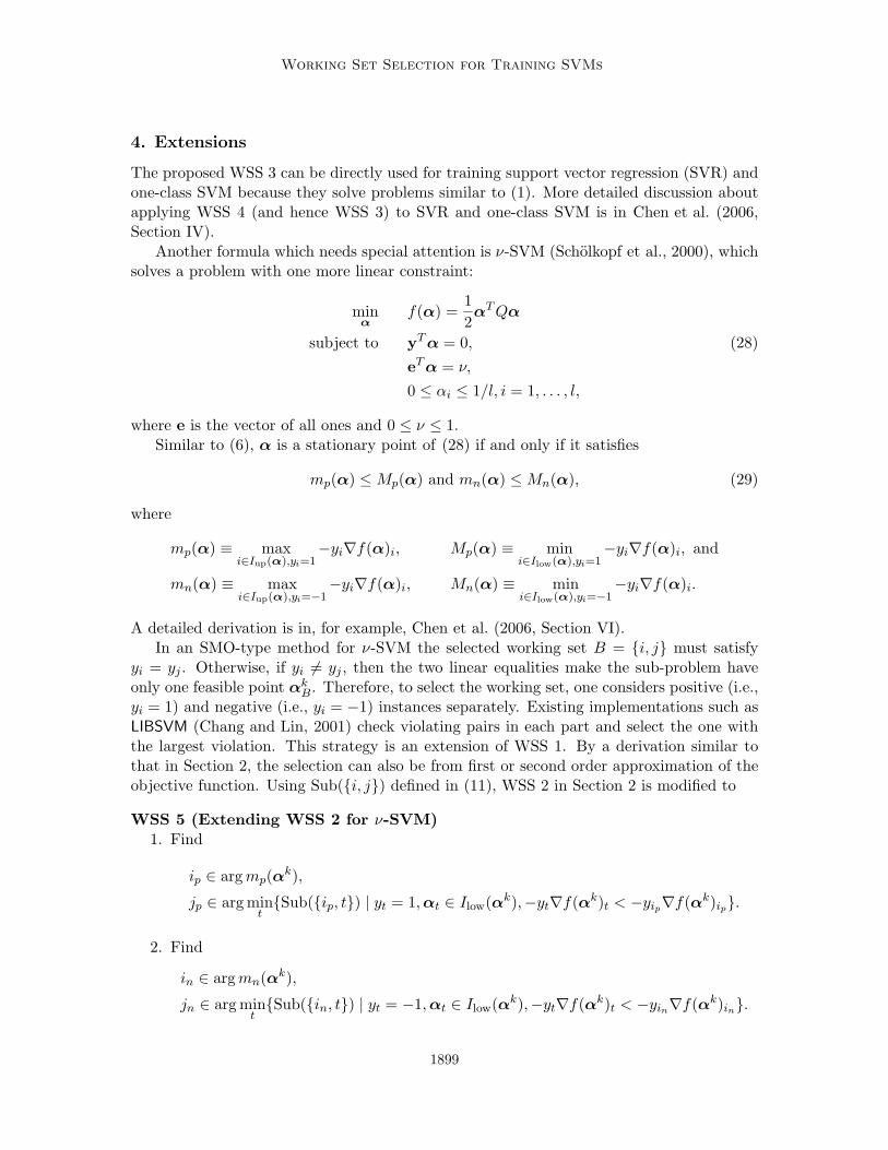
4. Extensions

The proposed WSS 3 can be directly used for training support vector regression (SVR) andone-class SVM because they solve problems similar to (1). More detailed discussion aboutapplying WSS 4 (and hence WSS 3) to SVR and one-class SVM is in Chen et al. (2006,Section IV).

Another formula which needs special attention is ν-SVM (Scholkopf et al., 2000), whichsolves a problem with one more linear constraint:

minα

f(α) =1

2αT Qα

subject to yT α = 0, (28)

eT α = ν,

0 ≤ αi ≤ 1/l, i = 1, . . . , l,

where e is the vector of all ones and 0 ≤ ν ≤ 1.Similar to (6), α is a stationary point of (28) if and only if it satisfies

mp(α) ≤ Mp(α) and mn(α) ≤ Mn(α), (29)

where

mp(α) ≡ maxi∈Iup(α),yi=1

−yi∇f(α)i, Mp(α) ≡ mini∈Ilow(α),yi=1

−yi∇f(α)i, and

mn(α) ≡ maxi∈Iup(α),yi=−1

−yi∇f(α)i, Mn(α) ≡ mini∈Ilow(α),yi=−1

−yi∇f(α)i.

A detailed derivation is in, for example, Chen et al. (2006, Section VI).In an SMO-type method for ν-SVM the selected working set B = {i, j} must satisfy

yi = yj . Otherwise, if yi 6= yj , then the two linear equalities make the sub-problem haveonly one feasible point αk

B. Therefore, to select the working set, one considers positive (i.e.,yi = 1) and negative (i.e., yi = −1) instances separately. Existing implementations such asLIBSVM (Chang and Lin, 2001) check violating pairs in each part and select the one withthe largest violation. This strategy is an extension of WSS 1. By a derivation similar tothat in Section 2, the selection can also be from first or second order approximation of theobjective function. Using Sub({i, j}) defined in (11), WSS 2 in Section 2 is modified to

WSS 5 (Extending WSS 2 for ν-SVM)1. Find

ip ∈ arg mp(αk),

jp ∈ arg mint{Sub({ip, t}) | yt = 1, αt ∈ Ilow(αk),−yt∇f(αk)t < −yip∇f(αk)ip}.

2. Find

in ∈ arg mn(αk),

jn ∈ arg mint{Sub({in, t}) | yt = −1, αt ∈ Ilow(αk),−yt∇f(αk)t < −yin∇f(αk)in}.

1899

Fan, Chen, and Lin

Problem #data #feat. Problem #data #feat. Problem #data #feat.

image 1,300 18 breast-cancer 690 10 abalone∗ 1,000 8splice 1,000 60 diabetes 768 8 cadata∗ 1,000 8tree 700 18 fourclass 862 2 cpusmall∗ 1,000 12a1a 1,605 119 german.numer 1,000 24 mg 1,385 6australian 683 14 w1a 2,477 300 space ga∗ 1,000 6

Table 1: Data statistics for small problems (left two columns: classification, right column:regression). ∗: subset of the original problem.

3. Check Sub({ip, jp}) and Sub({in, jn}). Return the set with a smaller value.

By Theorem 3 in Section 2, it is easy to solve Sub({ip, t}) and Sub({in, t}) in the aboveprocedure.

5. Experiments

In this section we aim at comparing the proposed WSS 3 with WSS 1, which selects themaximal violating pair. As indicated in Section 2, they differ only in finding the secondelement j: WSS 1 checks first order approximation of the objective function, but WSS 3uses second order information.

5.1 Data and Experimental Settings

First, some small data sets (around 1,000 samples) including ten binary classification andfive regression problems are investigated under various settings. Secondly, observations arefurther confirmed by using four large (more than 30,000 instances) classification problems.Data statistics are in Tables 1 and 3.

Problems german.numer and australian are from the Statlog collection (Michie et al.,1994). We select space ga and cadata from StatLib (http://lib.stat.cmu.edu/datasets).The data sets image, diabetes, covtype, breast-cancer, and abalone are from the UCI ma-chine learning repository (Newman et al., 1998). Problems a1a and a9a are compiled inPlatt (1998) from the UCI “adult” data set. Problems w1a and w8a are also from Platt(1998). The tree data set was originally used in Bailey et al. (1993). The problem mg isa Mackey-Glass time series. The data sets cpusmall and splice are from the Delve archive(http://www.cs.toronto.edu/~delve). Problem fourclass is from Ho and Kleinberg (1996)and we further transform it to a two-class set. The problem IJCNN1 is from the first problemof IJCNN 2001 challenge (Prokhorov, 2001).

For most data sets each attribute is linearly scaled to [−1, 1]. We do not scale a1a, a9a,w1a, and w8a as they take two values 0 and 1. Another exception is covtype, in which 44 of 54features have 0/1 values. We scale only the other ten features to [0, 1]. All data are availableat http://www.csie.ntu.edu.tw/~cjlin/libsvmtools/. We use LIBSVM (version 2.71)(Chang and Lin, 2001), an implementation of WSS 1, for experiments. An easy modificationto WSS 3 ensures that two codes differ only in the working set implementation. We setτ = 10−12 in WSS 3.

1900

http://lib.stat.cmu.edu/datasets

http://www.cs.toronto.edu/~delve

http://www.csie.ntu.edu.tw/~cjlin/libsvmtools/


Different SVM parameters such as C in (1) and kernel parameters affect the trainingtime. It is difficult to evaluate the two methods under every parameter setting. To havea fair comparison, we simulate how one uses SVM in practice and consider the followingprocedure:

1. “Parameter selection” step: Conduct five-fold cross validation to find the best onewithin a given set of parameters.

2. “Final training” step: Train the whole set with the best parameter to obtain the finalmodel.

For each step we check time and iterations using the two methods of working set selection.For some extreme parameters (e.g., very large or small values) in the “parameter selection”step, the decomposition method converges very slowly, so the comparison shows if theproposed WSS 3 saves time under difficult situations. On the other hand, the best parameterusually locates in a more normal region, so the “final training” step tests if WSS 3 iscompetitive with WSS 1 for easier cases.

The behavior of using different kernels is a concern, so we thoroughly test four commonlyused kernels:

1. RBF kernel:K(xi,xj) = e−γ‖xi−xj‖

2.

2. Linear kernel:K(xi,xj) = xT

i xj .

3. Polynomial kernel:K(xi,xj) = (γ(xT

i xj + 1))d.

4. Sigmoid kernel:K(xi,xj) = tanh(γxT

i xj + d).

Note that this function cannot be represented as φ(xi)T φ(xj) under some parameters.

Then the matrix Q is not positive semi-definite. Experimenting with this kernel testsif our extension to indefinite kernels in Section 2.3 works well or not.

Parameters used for each kernel are listed in Table 2. Note that as SVR has an additionalparameter ǫ, to save the running time, for other parameters we may not consider as manyvalues as in classification.

It is important to check how WSS 3 performs after incorporating shrinking and cachingstrategies. Such techniques may effectively save kernel evaluations at each iteration, so thehigher cost of WSS 3 is a concern. We consider various settings:

1. With or without shrinking.

2. Different cache size: First a 40MB cache allows the whole kernel matrix to be storedin the computer memory. Second, we allocate only 100K, so cache misses may happenand more kernel evaluations are needed. The second setting simulates the training oflarge-scale sets whose kernel matrices cannot be stored.

1901

Fan, Chen, and Lin

Kernel Problem type log2 C log2 γ log2 ǫ d

RBF Classification −5, 15, 2 3,−15,−2Regression −1, 15, 2 3,−15,−2 −8,−1, 1

Linear Classification −3, 5, 2Regression −3, 5, 2 −8,−1, 1

Polynomial Classification −3, 5, 2 −5,−1, 1 2, 4, 1Regression −3, 5, 2 −5,−1, 1 −8,−1, 1 2, 4, 1

Sigmoid Classification −3, 12, 3 −12, 3, 3 −2.4, 2.4, 0.6Regression −3, 9, 3 γ = 1

#features−8,−1, 3 −2.4, 2.4, 0.6

Table 2: Parameters used for various kernels: values of each parameter are from a uniformdiscretization of an interval. We list the left, right end points and the space fordiscretization. For example, −5, 15, 2 for log2 C means log2 C = −5,−3, . . . , 15.

5.2 Results

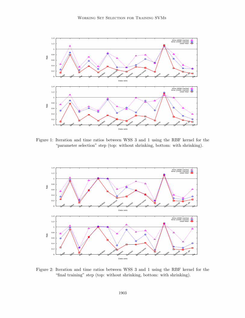
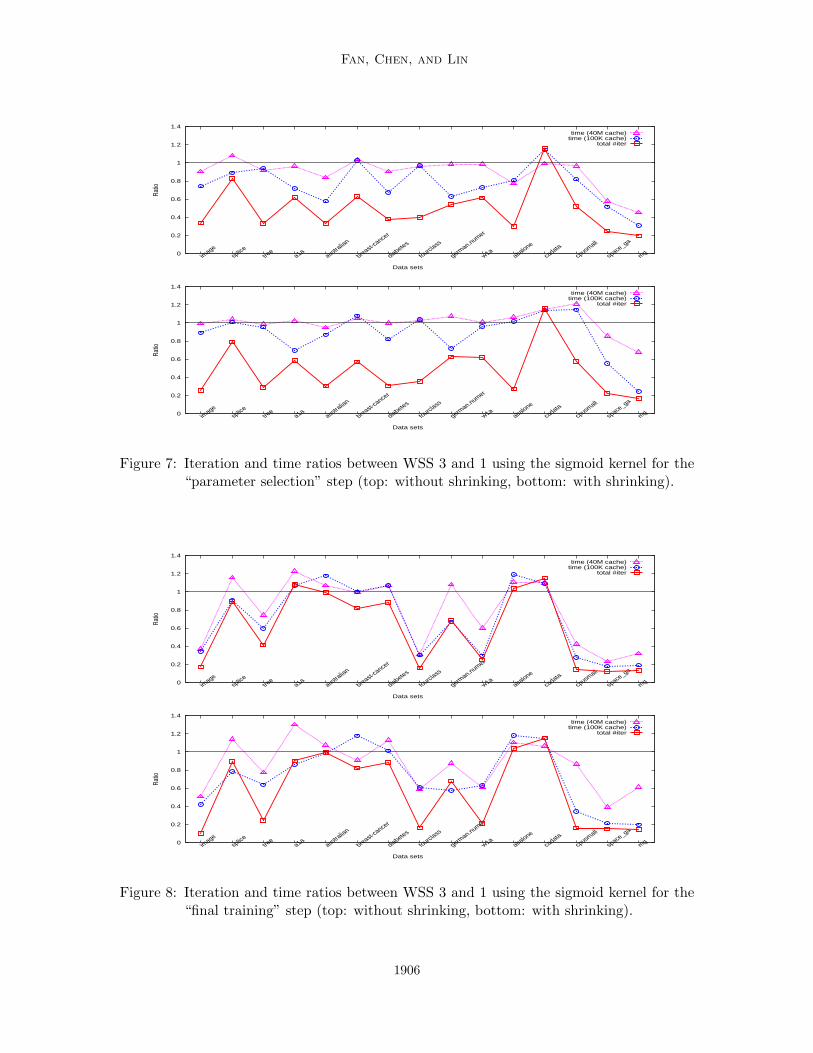
For each kernel, we give two figures showing results of “parameter selection” and “finaltraining” steps, respectively. We further separate each figure to two scenarios: without/withshrinking, and present three ratios between using WSS 3 and using WSS 1:

ratio 1 ≡# iter. by Alg. 2 with WSS 3

# iter. by Alg. 2 with WSS 1,

ratio 2 ≡time by Alg. 2 (WSS 3, 100K cache)

time by Alg. 2 (WSS 1, 100K cache),

ratio 3 ≡time by Alg. 2 (WSS 3, 40M cache)

time by Alg. 2 (WSS 1, 40M cache).

Note that the number of iterations is independent of the cache size. For the “parameterselection” step, time (or iterations) of all parameters is summed up before calculating theratio. In general the “final training” step is very fast, so the timing result may not beaccurate. Hence we repeat this step several times to obtain more reliable timing values.Figures 1-8 present obtained ratios. They are in general smaller than one, so using WSS 3is really better than using WSS 1. Before describing other results, we explain an interestingobservation: In these figures, if shrinking is not used, in general

ratio 1 ≤ ratio 2 ≤ ratio 3. (30)

Under the two very different cache sizes, one is too small to store the kernel matrix, butthe other is large enough. Thus, roughly we have

time per Alg. 2 iteration (100K cache) ≈ Calculating two Q columns + Selection,

time per Alg. 2 iteration (40M cache) ≈ Selection.

(31)

If shrinking is not used, the optimization problem is not reduced and hence

time by Alg. 2

# iter. of Alg. 2≈ cost per iteration ≈ constant. (32)

1902


0

0.2

0.4

0.6

0.8

1

1.2

1.4

image

splice

tree

a1aaustr

alian

breast-ca

ncer

diabetes

fourclass

german.numer

w1aabalone

cadata

cpusm

all

space

_ga

mg

Ratio

Data sets

time (40M cache)time (100K cache)

total #iter

0

0.2

0.4

0.6

0.8

1

1.2

1.4

image

splice

tree

a1aaustr

alian

breast-ca

ncer

diabetes

fourclass

german.numer

w1aabalone

cadata

cpusm

all

space

_ga

mg

Ratio

Data sets


total #iter

Figure 1: Iteration and time ratios between WSS 3 and 1 using the RBF kernel for the“parameter selection” step (top: without shrinking, bottom: with shrinking).

0

0.2

0.4

0.6

0.8

1

1.2

1.4

image

splice

tree

a1aaustr

alian

breast-ca

ncer

diabetes

fourclass

german.numer

w1aabalone

cadata

cpusm

all

space

_ga

mg

Ratio

Data sets


total #iter

0

0.2

0.4

0.6

0.8

1

1.2

1.4

image

splice

tree

a1aaustr

alian

breast-ca

ncer

diabetes

fourclass

german.numer

w1aabalone

cadata

cpusm

all

space

_ga

mg

Ratio

Data sets


total #iter

Figure 2: Iteration and time ratios between WSS 3 and 1 using the RBF kernel for the“final training” step (top: without shrinking, bottom: with shrinking).

1903

Fan, Chen, and Lin

0

0.2

0.4

0.6

0.8

1

1.2

1.4

image

splice

tree

a1aaustr

alian

breast-ca

ncer

diabetes

fourclass

german.numer

w1aabalone

cadata

cpusm

all

space

_ga

mg

Ratio

Data sets


total #iter

0

0.2

0.4

0.6

0.8

1

1.2

1.4

image

splice

tree

a1aaustr

alian

breast-ca

ncer

diabetes

fourclass

german.numer

w1aabalone

cadata

cpusm

all

space

_ga

mg

Ratio

Data sets


total #iter

Figure 3: Iteration and time ratios between WSS 3 and 1 using the linear kernel for the“parameter selection” step (top: without shrinking, bottom: with shrinking).

0

0.2

0.4

0.6

0.8

1

1.2

1.4

image

splice

tree

a1aaustr

alian

breast-ca

ncer

diabetes

fourclass

german.numer

w1aabalone

cadata

cpusm

all

space

_ga

mg

Ratio

Data sets


total #iter

0

0.2

0.4

0.6

0.8

1

1.2

1.4

image

splice

tree

a1aaustr

alian

breast-ca

ncer

diabetes

fourclass

german.numer

w1aabalone

cadata

cpusm

all

space

_ga

mg

Ratio

Data sets


total #iter

Figure 4: Iteration and time ratios between WSS 3 and 1 using the linear kernel for the“final training” step (top: without shrinking, bottom: with shrinking).

1904


0

0.2

0.4

0.6

0.8

1

1.2

1.4

image

splice

tree

a1aaustr

alian

breast-ca

ncer

diabetes

fourclass

german.numer

w1aabalone

cadata

cpusm

all

space

_ga

mg

Ratio

Data sets


total #iter

0

0.2

0.4

0.6

0.8

1

1.2

1.4

image

splice

tree

a1aaustr

alian

breast-ca

ncer

diabetes

fourclass

german.numer

w1aabalone

cadata

cpusm

all

space

_ga

mg

Ratio

Data sets


total #iter

Figure 5: Iteration and time ratios between WSS 3 and 1 using the polynomial kernel forthe “parameter selection” step (top: without shrinking, bottom: with shrinking).

0

0.2

0.4

0.6

0.8

1

1.2

1.4

image

splice

tree

a1aaustr

alian

breast-ca

ncer

diabetes

fourclass

german.numer

w1aabalone

cadata

cpusm

all

space

_ga

mg

Ratio

Data sets


total #iter

0

0.2

0.4

0.6

0.8

1

1.2

1.4

image

splice

tree

a1aaustr

alian

breast-ca

ncer

diabetes

fourclass

german.numer

w1aabalone

cadata

cpusm

all

space

_ga

mg

Ratio

Data sets


total #iter

Figure 6: Iteration and time ratios between WSS 3 and 1 using the polynomial kernel forthe “final training” step (top: without shrinking, bottom: with shrinking).

1905

Fan, Chen, and Lin

0

0.2

0.4

0.6

0.8

1

1.2

1.4

image

splice

tree

a1aaustr

alian

breast-ca

ncer

diabetes

fourclass

german.numer

w1aabalone

cadata

cpusm

all

space

_ga

mg

Ratio

Data sets


total #iter

0

0.2

0.4

0.6

0.8

1

1.2

1.4

image

splice

tree

a1aaustr

alian

breast-ca

ncer

diabetes

fourclass

german.numer

w1aabalone

cadata

cpusm

all

space

_ga

mg

Ratio

Data sets


total #iter

Figure 7: Iteration and time ratios between WSS 3 and 1 using the sigmoid kernel for the“parameter selection” step (top: without shrinking, bottom: with shrinking).

0

0.2

0.4

0.6

0.8

1

1.2

1.4

image

splice

tree

a1aaustr

alian

breast-ca

ncer

diabetes

fourclass

german.numer

w1aabalone

cadata

cpusm

all

space

_ga

mg

Ratio

Data sets


total #iter

0

0.2

0.4

0.6

0.8

1

1.2

1.4

image

splice

tree

a1aaustr

alian

breast-ca

ncer

diabetes

fourclass

german.numer

w1aabalone

cadata

cpusm

all

space

_ga

mg

Ratio

Data sets


total #iter

Figure 8: Iteration and time ratios between WSS 3 and 1 using the sigmoid kernel for the“final training” step (top: without shrinking, bottom: with shrinking).

1906


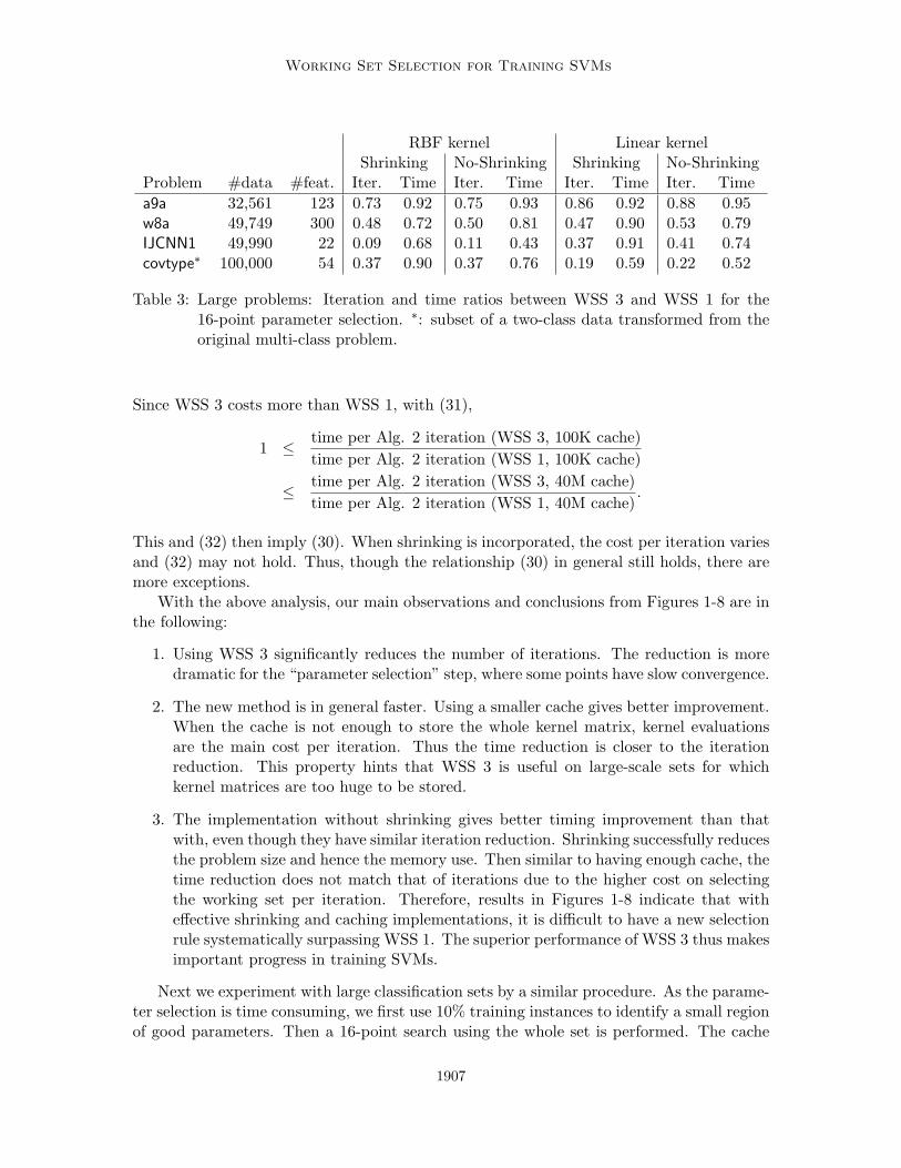
RBF kernel Linear kernelShrinking No-Shrinking Shrinking No-Shrinking

Problem #data #feat. Iter. Time Iter. Time Iter. Time Iter. Time

a9a 32,561 123 0.73 0.92 0.75 0.93 0.86 0.92 0.88 0.95w8a 49,749 300 0.48 0.72 0.50 0.81 0.47 0.90 0.53 0.79IJCNN1 49,990 22 0.09 0.68 0.11 0.43 0.37 0.91 0.41 0.74covtype∗ 100,000 54 0.37 0.90 0.37 0.76 0.19 0.59 0.22 0.52

Table 3: Large problems: Iteration and time ratios between WSS 3 and WSS 1 for the16-point parameter selection. ∗: subset of a two-class data transformed from theoriginal multi-class problem.

Since WSS 3 costs more than WSS 1, with (31),

1 ≤time per Alg. 2 iteration (WSS 3, 100K cache)

time per Alg. 2 iteration (WSS 1, 100K cache)

≤time per Alg. 2 iteration (WSS 3, 40M cache)

time per Alg. 2 iteration (WSS 1, 40M cache).

This and (32) then imply (30). When shrinking is incorporated, the cost per iteration variesand (32) may not hold. Thus, though the relationship (30) in general still holds, there aremore exceptions.

With the above analysis, our main observations and conclusions from Figures 1-8 are inthe following:

1. Using WSS 3 significantly reduces the number of iterations. The reduction is moredramatic for the “parameter selection” step, where some points have slow convergence.

2. The new method is in general faster. Using a smaller cache gives better improvement.When the cache is not enough to store the whole kernel matrix, kernel evaluationsare the main cost per iteration. Thus the time reduction is closer to the iterationreduction. This property hints that WSS 3 is useful on large-scale sets for whichkernel matrices are too huge to be stored.

3. The implementation without shrinking gives better timing improvement than thatwith, even though they have similar iteration reduction. Shrinking successfully reducesthe problem size and hence the memory use. Then similar to having enough cache, thetime reduction does not match that of iterations due to the higher cost on selectingthe working set per iteration. Therefore, results in Figures 1-8 indicate that witheffective shrinking and caching implementations, it is difficult to have a new selectionrule systematically surpassing WSS 1. The superior performance of WSS 3 thus makesimportant progress in training SVMs.

Next we experiment with large classification sets by a similar procedure. As the parame-ter selection is time consuming, we first use 10% training instances to identify a small regionof good parameters. Then a 16-point search using the whole set is performed. The cache

1907

Fan, Chen, and Lin

size is 350M except 800M for covtype. We experiment with RBF and linear kernels. Table3 gives iteration and time ratios of conducting the 16-point parameter selection. Similar toresults for small problems, the number of iterations using WSS 3 is much smaller than thatof using WSS 1. The training time of using WSS 3 is also shorter.

6. Maintaining Feasibility in Sub-problems for Working Set Selections

In Section 2, both the linear sub-problem (8) and quadratic sub-problem (11) do not requireαk +d to be feasible. One may wonder if enforcing the feasibility gives a better working setand hence leads to faster convergence. In this situation, the quadratic sub-problem becomes

Sub(B) ≡ mindB

1

2dT


BdB

subject to yTBdB = 0, (33)

−αkt ≤ dt ≤ C − αk

t ,∀t ∈ B.

For example, from some candidate pairs, Lai et al. (2003a,b) select the one with the smallestvalue of (33) as the working set. To check the effect of using (33), here we replace (11) inWSS 2 with (33) and compare it with the original WSS 2.

From (9), a nice property of using (33) is that Sub(B) equals the decrease of the objectivefunction f by moving from αk to another feasible point αk+d. In fact, once B is determined,(33) is also the sub-problem (2) used in Algorithm 1 to obtain αk+1. Therefore, we use thesame sub-problem for both selecting the working set and obtaining the next iteration αk+1.One may think that such a selection method is better as it leads to the largest functionvalue reduction while maintaining the feasibility. However, solving (33) is more expensivethan (11) since checking the feasibility requires additional effort. To be more precise, ifB = {i, j}, using dj = −di = yjdj = −yidi and a derivation similar to (13), we now must

minimize 12 aij d

2j + bij dj under the constraints

− αkj ≤ dj = yj dj ≤ C − αk

j and − αki ≤ di = −yidj ≤ C − αk

i . (34)

As the minimum of the objective function happens at −bij/aij , to have a solution satisfying(34), we multiply it by −yi and check the second constraint. Next, by dj = −yiyjdi, wecheck the first constraint. Equation (20) in WSS 3 is thus modified to

j ∈ arg mint

{

1

2aitd

2t + bitdt | t ∈ Ilow(αk),−yt∇f(αk)t < −yi∇f(αk)i,

dt = yt max(−αkt , min(C − αk

t ,−ytyi max(−αki , min(C − αk

i , yibit/ait))))}

.

(35)

Clearly (35) requires more operations than (20).

In this section, we prove that under some minor assumptions, in final iterations, solving(11) in WSS 2 is the same as solving (33). This result and experiments then indicate thatthere is no need to use the more sophisticated sub-problem (33) for selecting working sets.

1908


0.6

0.7

0.8

0.9

1

1.1

1.2

1.3

1.4

imag

e

splic

e

tree

a1a

austr

alian

brea

st-ca

ncer

diabe

tes

four

class

germ

an.n

umer

w1a abalo

ne

cada

ta

cpus

mall

spac

e_ga

mg

Ratio

Data sets


total #iter

(a) The “parameter selection” step without shrinking

0.6

0.7

0.8

0.9

1

1.1

1.2

1.3

1.4

imag

e

splic

e

tree

a1a

austr

alian

brea

st-ca

ncer

diabe

tes

four

class

germ

an.n

umer

w1a abalo

ne

cada

ta

cpus

mall

spac

e_ga

mg

Ratio

Data sets


total #iter

(b) The “final training” step without shrinking

0.6

0.7

0.8

0.9

1

1.1

1.2

1.3

1.4

imag

e

splic

e

tree

a1a

austr

alian

brea

st-ca

ncer

diabe

tes

four

class

germ

an.n

umer

w1a abalo

ne

cada

ta

cpus

mall

spac

e_ga

mg

Ratio

Data sets


total #iter

(c) The “parameter selection” step with shrinking

0.6

0.7

0.8

0.9

1

1.1

1.2

1.3

1.4

imag

e

splic

e

tree

a1a

austr

alian

brea

st-ca

ncer

diabe

tes

four

class

germ

an.n

umer

w1a abalo

ne

cada

ta

cpus

mall

spac

e_ga

mg

Ratio

Data sets


total #iter

(d) The “final training” step with shrinking

Figure 9: Iteration and time ratios between using (11) and (33) in WSS 2. Note that theratio (y-axis) starts from 0.6 but not 0.

6.1 Solutions of (11) and (33) in final iterations

Theorem 7 Let {αk} be the infinite sequence generated by the SMO-type decompositionmethod using WSS 2. Under the same assumptions of Theorem 6, there is k such that fork ≥ k, WSS 2 returns the same working set by replacing (11) with (33).

Proof Since K is assumed to be positive definite, problem (1) has a unique optimal solutionα. Using Theorem 4,

limk→∞

αk = α. (36)

Since {αk} is an infinite sequence, Theorem 5 shows that m(α) = M(α). Hence we candefine the following set

I ′ ≡ {t | −yt∇f(α)t = m(α) = M(α)}.

1909

Fan, Chen, and Lin

As α is a non-degenerate point, from (27),

δ ≡ mint∈I′

(αt, C − αt) > 0.

Using 1) Eq. (36), 2) ∇f(α)i = ∇f(α)j ,∀i, j ∈ I ′, and 3) Eq. (25) of Theorem 5, there isk such that for all k ≥ k,

|αki − αi| <

δ

2,∀i ∈ I ′, (37)

| − yi∇f(αk)i + yj∇f(αk)j |

Kii + Kjj − 2Kij<

δ

2,∀i, j ∈ I ′, Kii + Kjj − 2Kij > 0, (38)

andall violating pairs come from I ′. (39)

For any given index pair B, let Sub(11)(B) and Sub(33)(B) denote the optimal objectivevalues of (11) and (33), respectively. If B = {i, j} is a violating pair selected by WSS 2 atthe kth iteration, (37)-(39) imply that di and dj defined in (15) satisfy

0 < αk+1i = αk

i + di < C and 0 < αk+1j = αk

j + dj < C. (40)

Therefore, the optimal dB of (11) is feasible for (33). That is,

Sub(33)(B) ≤ Sub(11)(B). (41)

Since (33)’s constraints are stricter than those of (11), we have

Sub(11)(B) ≤ Sub(33)(B),∀B. (42)

From WSS 3,

j ∈ arg mint{Sub(11)({i, t}) | t ∈ Ilow(αk),−yt∇f(αk)t < −yi∇f(αk)i}.

With (41) and (42), this j satisfies

j ∈ arg mint{Sub(33)({i, t}) | t ∈ Ilow(αk),−yt∇f(αk)t < −yi∇f(αk)i}.

Therefore, replacing (11) in WSS 3 with (33) does not affect the selected working set.

This theorem indicates that the two methods of working set selection in general lead toa similar number of iterations. As (11) does not check the feasibility, the implementationof using it should be faster.

6.2 Experiments

Under the framework WSS 2, we conduct experiments to check if using (11) is really fasterthan using (33). The same data sets in Section 5 are used under the same setting. Forsimplicity, we consider only the RBF kernel.

1910


Similar to figures in Section 5, here Figure 9 presents iteration and time ratios betweenusing (11) and (33):

# iter. by using (11)

# iter. by using (33),time by using (11) (100K cache)

time by using (33) (100K cache),time by using (11) (40M cache)

time by using (33) (40M cache).

Without shrinking, clearly both approaches have very similar numbers of iterations.This observation is expected due to Theorem 7. Then as (33) costs more than (11) does,the time ratio is in general smaller than one. Especially when the cache is large enoughto store all kernel elements, selecting working sets is the main cost and hence the ratio islower.

With shrinking, in Figures 9(c) and 9(d), the iteration ratio is larger than one forseveral problems. Surprisingly, the time ratio, especially that of using a small cache, is evensmaller than that without shrinking. In other words, (11) better incorporates the shrinkingtechnique than (33) does. To analyze this observation, we check the number of removedvariables along iterations, and find that (11) leads to more aggressive shrinking. Then thereduced problem can be stored in the small cache (100K), so kernel evaluations are largelysaved. Occasionally the shrinking is too aggressive so some variables are wrongly removed.Then recovering from mistakes causes longer iterations.

Note that our shrinking implementation is by removing bounded elements not in theset (25). Thus, the smaller the interval [M(αk), m(αk)] is, the more variables are shrunk.In Figure 10, we show the relationship between the maximal violation m(αk)−M(αk) anditerations. Clearly using (11) reduces the maximal violation more quickly than using (33).A possible explanation is that (11) has less restriction than (33): In early iterations, if a setB = {i, j} is associated with a large violation −yi∇f(αk)i +yj∇f(αk)j , then dB defined in(15) has large components. Hence though it minimizes the quadratic functions (9), αk

B +dB

is easily infeasible. To solve (33), one thus changes αkB + dB back to the feasible region

as (35) does. As a reduced step is taken, the corresponding Sub(B) may not be smallerthan those of using other sets. On the other hand, (11) does not require αk

B + dB to befeasible, so a large step is taken. The resulting Sub(B) thus may be small enough so thatB is selected. Therefore, using (11) tend to select working sets with large violations andhence may more quickly reduce the maximal violation.

Discussion here shows that (11) is better than (33). They lead to similar numbers ofiterations, but the cost per iteration is less by using (11). Moreover, (11) better incorporatesthe shrinking technique.

6.3 Sub-problems Using First Order Information

Under first order approximation, we can also modify the sub-problem (8) to the followingform, which maintains the feasibility:

Sub(B) ≡ mindB

∇f(αk)TBdB

subject to yTBdB = 0, (43)

0 ≤ αi + di ≤ C, i ∈ B.

1911

Fan, Chen, and Lin

0

5

10

15

20

25

0 10000 20000 30000 40000 50000 60000 70000

(11)(33)

(a) tree

0

0.2

0.4

0.6

0.8

1

1.2

1.4

1.6

1.8

0 200 400 600 800 1000 1200 1400 1600

(11)(33)

(b) splice

0

2

4

6

8

10

12

14

0 1000 2000 3000 4000 5000 6000 7000 8000 9000

(11)(33)

(c) diabetes

0

1

2

3

4

5

6

0 5000 10000 15000 20000 25000 30000

(11)(33)

(d) german.numer

Figure 10: Iterations (x-axis) and maximal violations (y-axis) of using (11) and (33).

Section 2 discusses that a maximal violating pair is an optimal solution of minB:|B|=2 Sub(B),where Sub(B) is (8). If (43) is used instead, Simon (2004) has shown an O(l) procedure toobtain a solution. Thus the time complexity is the same as that of using (8).

Note that Theorem 7 does not hold for these two selection methods. In the proof, weuse the small changes of αk

i in final iterations to show that certain αki never reaches bounds

0 and C. Then the sub-problem (2) to find αk+1 is indeed the best sub-problem obtainedin the procedure of working set selection. Now no matter (8) or (43) is used for selectingthe working set, we still use (2) to find αk+1. Therefore, we cannot link the small changebetween αk and αk+1 to the optimal dB in the procedure of working set selection. Withoutan interpretation like Theorem 7, the performance difference between using (8) and (43)remains unclear and is a future research issue.

7. Discussion and Conclusions

In Section 2, the selection (10) of using second order information may involve checking(

l2

)

pairs of indices. This is not practically viable, so in WSS 2 we heuristically fix i ∈ arg m(αk)and examine O(l) sets to find j. It is interesting to see how well this heuristic performsand whether we can make further improvements. By running the same small classificationproblems used in Section 6, Figure 11 presents the iteration ratio between using two selectionmethods:

# iter. by Alg. 2 and checking(

l2

)

pairs

# iter. by Alg. 2 and WSS 2.

1912


0.4

0.5

0.6

0.7

0.8

0.9

1

1.1

1.2

1.3

1.4

image

splic

etre

ea1a

australia

n

breast-ca

ncer

diabetes

fourclass

german.numer

w1a

Ratio

Data sets

parameter selectionfinal training

(a) RBF kernel

0.4

0.5

0.6

0.7

0.8

0.9

1

1.1

1.2

1.3

1.4

image

splic

etre

ea1a

australia

n

breast-ca

ncer

diabetes

fourclass

german.numer

w1a

Ratio

Data sets

parameter selectionfinal training

(b) Linear kernel

Figure 11: Iteration ratios between using two selection methods: checking all(

l2

)

pairs andWSS 2. Note that the ratio (y-axis) starts from 0.4 but not 0.

We do not use shrinking and consider both RBF and linear kernels. Figure 11 clearly showsthat a full check of all index pairs causes fewer iterations. However, as the average of ratiosfor various problems is between 0.7 and 0.8, this selection reduces iterations of using WSS 2by only 20% to 30%. Therefore, WSS 2, an O(l) procedure, successfully returns a workingset nearly as good as that by an O(l2) procedure. In other words, the O(l) sets heuristicallyconsidered in WSS 2 are among the best in all

(

l2

)

candidates.

Experiments in this paper fully demonstrate that using the proposed WSS 2 (and henceWSS 3) leads to faster convergence (i.e., fewer iterations) than using WSS 1. This resultis reasonable as the selection based on second order information better approximates theobjective function in each iteration. However, this argument explains only the behaviorper iteration, but not the global performance of the decomposition method. A theoreticalstudy showing that the proposed selection leads to better convergence rates is a difficultbut interesting future issue.

In summary, we have proposed a new and effective working set selection WSS 3. TheSMO-type decomposition method using it asymptotically converges and satisfies other usefultheoretical properties. Experiments show that it is better than a commonly used selectionWSS 1, in both the training time and iterations.

WSS 3 has replaced WSS 1 in the software LIBSVM (after version 2.8).

1913

Fan, Chen, and Lin

Acknowledgments

This work was supported in part by the National Science Council of Taiwan via the grantNSC 93-2213-E-002-030.

Appendix A. WSS 1 Solves Problem (7): the Proof

For any given {i, j}, we can substitute di ≡ yidi and dj ≡ yjdj to (8), so the objectivefunction becomes

(−yi∇f(αk)i + yj∇f(αk)j)dj . (44)

As di = dj = 0 is feasible for (8), the minimum of (44) is zero or a negative number. If

−yi∇f(αk)i > −yj∇f(αk)j , using the condition di + dj = 0, the only possibility for (44) to

be negative is dj < 0 and di > 0. From (3), (8b), and (8c), this corresponds to i ∈ Iup(αk)

and j ∈ Ilow(αk). Moreover, the minimum occurs at dj = −1 and di = 1. The situation of−yi∇f(αk)i < −yj∇f(αk)j is similar.

Therefore, solving (7) is essentially the same as

min{

min(

yi∇f(αk)i − yj∇f(αk)j , 0)

∣

∣ i ∈ Iup(αk), j ∈ Ilow(αk)

}

= min(

−m(αk) + M(αk), 0)

.

Hence, if there are violating pairs, the maximal one solves (7).

Appendix B. Pseudo Code of Algorithm 2 and WSS 3

B.1 Main Program (Algorithm 2)

Inputs:

y: array of {+1, -1}: class of the i-th instance

Q: Q[i][j] = y[i]*y[j]*K[i][j]; K: kernel matrix

len: number of instances

// parameters

eps = 1e-3 // stopping tolerance

tau = 1e-12

// main routine

initialize alpha array A to all zero

initialize gradient array G to all -1

while (1) {

(i,j) = selectB()

if (j == -1)

break

// working set is (i,j)

a = Q[i][i]+Q[j][j]-2*y[i]*y[j]*Q[i][j]

if (a <= 0)

a = tau

1914


b = -y[i]*G[i]+y[j]*G[j]

// update alpha

oldAi = A[i], oldAj = A[j]

A[i] += y[i]*b/a

A[j] -= y[j]*b/a

// project alpha back to the feasible region

sum = y[i]*oldAi+y[j]*oldAj

if A[i] > C

A[i] = C

if A[i] < 0

A[i] = 0

A[j] = y[j]*(sum-y[i]*A[i])

if A[j] > C

A[j] = C

if A[j] < 0

A[j] = 0

A[i] = y[i]*(sum-y[j]*A[j])

// update gradient

deltaAi = A[i] - oldAi, deltaAj = A[j] - oldAj

for t = 1 to len

G[t] += Q[t][i]*deltaAi+Q[t][j]*deltaAj

}

B.2 Working Set Selection Subroutine (WSS 3)

// return (i,j)

procedure selectB

// select i

i = -1

G_max = -infinity

G_min = infinity

for t = 1 to len {

if (y[t] == +1 and A[t] < C) or

(y[t] == -1 and A[t] > 0) {

if (-y[t]*G[t] >= G_max) {

i = t

G_max = -y[t]*G[t]

}

}

}

// select j

j = -1

obj_min = infinity

for t = 1 to len {

if (y[t] == +1 and A[t] > 0) or

(y[t] == -1 and A[t] < C) {

b = G_max + y[t]*G[t]

1915

Fan, Chen, and Lin

if (-y[t]*G[t] <= G_min)

G_min = -y[t]*G[t]

if (b > 0) {

a = Q[i][i]+Q[t][t]-2*y[i]*y[t]*Q[i][t]

if (a <= 0)

a = tau

if (-(b*b)/a <= obj_min) {

j = t

obj_min = -(b*b)/a

}

}

}

}

if (G_max-G_min < eps)

return (-1,-1)

return (i,j)

end procedure

References

R. R. Bailey, E. J. Pettit, R. T. Borochoff, M. T. Manry, and X. Jiang. Automatic recog-nition of usgs land use/cover categories using statistical and neural networks classifiers.In SPIE OE/Aerospace and Remote Sensing, Bellingham, WA, 1993. SPIE.

Bernhard E. Boser, Isabelle Guyon, and Vladimir Vapnik. A training algorithm for opti-mal margin classifiers. In Proceedings of the Fifth Annual Workshop on ComputationalLearning Theory, pages 144–152. ACM Press, 1992.

Chih-Chung Chang and Chih-Jen Lin. LIBSVM: a library for support vector machines,2001. Software available at http://www.csie.ntu.edu.tw/~cjlin/libsvm.

Pai-Hsuen Chen, Rong-En Fan, and Chih-Jen Lin. A study on SMO-type decompositionmethods for support vector machines. IEEE Transactions on Neural Networks, 17:893–908, July 2006. URL http://www.csie.ntu.edu.tw/~cjlin/papers/generalSMO.pdf.

Corina Cortes and Vladimir Vapnik. Support-vector network. Machine Learning, 20:273–297, 1995.

Tin Kam Ho and Eugene M. Kleinberg. Building projectable classifiers of arbitrary com-plexity. In Proceedings of the 13th International Conference on Pattern Recognition, pages880–885, Vienna, Austria, August 1996.

Don Hush and Clint Scovel. Polynomial-time decomposition algorithmsfor support vector machines. Machine Learning, 51:51–71, 2003. URLhttp://www.c3.lanl.gov/~dhush/machine_learning/svm_decomp.ps.

Thorsten Joachims. Making large-scale SVM learning practical. In Bernhard Scholkopf,Christopher J. C. Burges, and Alexander J. Smola, editors, Advances in Kernel Methods- Support Vector Learning, Cambridge, MA, 1998. MIT Press.

1916

http://www.csie.ntu.edu.tw/~cjlin/libsvm

http://www.csie.ntu.edu.tw/~cjlin/papers/generalSMO.pdf

http://www.c3.lanl.gov/~dhush/machine_learning/svm_decomp.ps


S. S. Keerthi, S. K. Shevade, C. Bhattacharyya, and K. R. K. Murthy. Improvements toPlatt’s SMO algorithm for SVM classifier design. Neural Computation, 13:637–649, 2001.

D. Lai, N. Mani, and M. Palaniswami. Increasing the step of the Newtonian decompositionmethod for support vector machines. Technical Report MECSE-29-2003, Dept. Electricaland Computer Systems Engineering Monash University, Australia, 2003a.

D. Lai, N. Mani, and M. Palaniswami. A new method to select working sets for fastertraining for support vector machines. Technical Report MESCE-30-2003, Dept. Electricaland Computer Systems Engineering Monash University, Australia, 2003b.

Chih-Jen Lin. On the convergence of the decomposition method for support vectormachines. IEEE Transactions on Neural Networks, 12(6):1288–1298, 2001a. URLhttp://www.csie.ntu.edu.tw/~cjlin/papers/conv.ps.gz.

Chih-Jen Lin. Asymptotic convergence of an SMO algorithm without any as-sumptions. IEEE Transactions on Neural Networks, 13(1):248–250, 2002. URLhttp://www.csie.ntu.edu.tw/~cjlin/papers/q2conv.pdf.

Chih-Jen Lin. Linear convergence of a decomposition method for support vector machines.Technical report, Department of Computer Science, National Taiwan University, 2001b.URL http://www.csie.ntu.edu.tw/~cjlin/papers/linearconv.pdf.

D. Michie, D. J. Spiegelhalter, and C. C. Taylor. Machine Learning, Neural and Sta-tistical Classification. Prentice Hall, Englewood Cliffs, N.J., 1994. Data available athttp://www.ncc.up.pt/liacc/ML/statlog/datasets.html.

D. J. Newman, S. Hettich, C. L. Blake, and C. J. Merz. UCI repos-itory of machine learning databases. Technical report, University of Cal-ifornia, Irvine, Dept. of Information and Computer Sciences, 1998. URLhttp://www.ics.uci.edu/~mlearn/MLRepository.html.

E. Osuna, R. Freund, and F. Girosi. Training support vector machines: An application toface detection. In Proceedings of CVPR’97, pages 130–136, New York, NY, 1997. IEEE.

Laura Palagi and Marco Sciandrone. On the convergence of a modified version of SVMlight

algorithm. Optimization Methods and Software, 20(2-3):315–332, 2005.

John C. Platt. Fast training of support vector machines using sequential minimal opti-mization. In Bernhard Scholkopf, Christopher J. C. Burges, and Alexander J. Smola,editors, Advances in Kernel Methods - Support Vector Learning, Cambridge, MA, 1998.MIT Press.

Danil Prokhorov. IJCNN 2001 neural network competition. Slide presentation in IJCNN’01,Ford Research Laboratory, 2001. http://www.geocities.com/ijcnn/nnc_ijcnn01.pdf.

B. Scholkopf, A. Smola, R. C. Williamson, and P. L. Bartlett. New support vector algo-rithms. Neural Computation, 12:1207–1245, 2000.

1917

http://www.csie.ntu.edu.tw/~cjlin/papers/conv.ps.gz

http://www.csie.ntu.edu.tw/~cjlin/papers/q2conv.pdf

http://www.csie.ntu.edu.tw/~cjlin/papers/linearconv.pdf

http://www.ncc.up.pt/liacc/ML/statlog/datasets.html

http://www.ics.uci.edu/~mlearn/MLRepository.html

Fan, Chen, and Lin

Hans Ulrich Simon. On the complexity of working set selection. In Proceedings of the 15thInternational Conference on Algorithmic Learning Theory (ALT 2004), 2004.

1918

working set selection using second order information …cjlin/papers/quadworkset.pdf · working set...

Documents