working paper series - ecb.europa.eu · abstract we study the impact of increasingly negative...

Working Paper Series Do negative interest rates make banks less safe?

Federico Nucera, Andre Lucas, Julia Schaumburg, Bernd Schwaab

Disclaimer: This paper should not be reported as representing the views of the European Central Bank (ECB). The views expressed are those of the authors and do not necessarily reflect those of the ECB.

No 2098 / September 2017

Abstract

We study the impact of increasingly negative central bank policy rates on banks’

propensity to become undercapitalized in a financial crisis (‘SRisk’). We find that

the risk impact of negative rates is moderate, and depends on banks’ business models:

Banks with diversified income streams are perceived by the market as less risky, while

banks that rely predominantly on deposit funding are perceived as more risky. Policy

rate cuts below zero trigger different SRisk responses than an earlier cut to zero.

Keywords: negative interest rates; bank business model; systemic risk; unconven-

tional monetary policy measures

JEL classifications: G20, G21

ECB Working Paper 2098, September 2017 1

Non-technical summary

Since the onset of the financial crisis in 2007, many central banks have implemented

unprecedented standard and non-standard monetary policy measures, lowering key inter-

est rates to approximately zero. To stimulate post-crisis economies characterized by low

growth and low inflation, some central banks, including the European Central Bank (ECB),

have even adopted negative policy rates. The rationale for negative rates is that they pro-

vide additional monetary stimulus, and in this way support growth and a return to target

inflation.

Negative rates, by stimulating the economy, could be beneficial for financial institutions

via an increase in loan demand, improved asset quality, and a reduced riskiness of loans. On

the other hand, two main concerns have been voiced by critics of negative policy rates. First,

negative rates could also put pressure on the profitability of financial institutions. Banks

may therefore lend to riskier borrowers (‘risk shifting’). Second, a ‘search for yield’ among

institutional investors could lead to a disproportional demand for high-yielding risky assets.

If so, the implied asset price inflation could impair financial stability.

Which types of banks are perceived by markets as more or less risky at negative rates is as

yet unclear. In addition, it is currently unknown whether cuts to negative rates are ‘special’,

for example because they imply a different financial stability impact than comparable cuts

to low but non-negative rates. In this paper we contribute to answering these questions. To

do so, we study the risk impact as perceived by markets of three successive deposit facility

rate (DFR) cuts by the ECB to negative values, each by 10 basis points (bps) on June 5,

2014, September 4, 2014, and December 3, 2015. Furthermore, we examine whether the

impact of these cuts is qualitatively different from an earlier cut of the DFR from 25 bps to

zero on July 5, 2012.

We focus on banks’ risks of being undercapitalized in a potential future stress scenario

as measured by ‘SRisk’. SRisk is the estimated capital shortfall of a bank, conditional

on a 40% drop in a world equity index over a six months-ahead horizon. The measure is

modelled as a function of a bank’s equity market valuation, leverage ratio, the volatility of

its stock price, and the correlation of its stock price with the world index. SRisk does not

measure unconditional default risk, but instead mimics a market-based stress test. SRisk


estimates are available for 44 listed euro area banks at a monthly frequency. To ensure

a representative sample, and to include more banks in our analysis, we apply a matching

procedure to infer SRisk for non-listed banks. Specifically, we match 67 non-listed banks to

‘nearest neighboring’ banks for which market data are available. The matching is based on

accounting data, which are available for all 111 banks.

SRisk in the euro area falls markedly between mid-2012 and mid-2014, possibly initially

sparked by the ECB’s announcement of Outright Monetary Transactions in August 2012

and subsequently driven by the gradual recovery in economic growth and improving bank

capital buffers. Given pronounced variation in the level of SRisk for all banks, the impact

of the three DFR cuts to negative rates is of a relatively small(er) magnitude.

Using panel regressions we find that after a cut to an increasingly negative interest

rate, some, but not all, banks are perceived as more risky, i.e., more prone to become

undercapitalized in a potential future financial crisis. The risk impact depends on banks’

business models. Banks with sufficiently diversified income streams are perceived to be

less (systemically) risky. Such banks appear to benefit in net terms from negative rates.

By contrast, banks that rely predominantly on deposit funding are perceived by markets as

potentially more risky. The documented heterogeneity is in line with other studies that argue

that bank characteristics become an important determinant of monetary policy transmission

at negative rates.

Finally, a ‘placebo’ DFR cut from +25 bps to zero in July 2012 triggered different SRisk

responses than the 2014 and 2015 cuts below zero. This suggests that cuts to negative

rates may be ‘special’ in that they have a different financial stability impact than more

conventional cuts to non-negative rates.

Our regression results remain qualitatively similar if only listed banks are included in the

sample. The differential effects, however, become statistically insignificant in this case. The

results for non-listed banks should therefore be taken as tentative.


1 Introduction

Exceptional times can require exceptional policy measures. Since the onset of the financial

crisis in 2007, many central banks have implemented unprecedented standard and non-

standard monetary policy measures, lowering key interest rates to approximately zero. To

stimulate post-crisis economies characterized by low growth and low inflation, some central

banks, including the European Central Bank (ECB) and the central banks of Denmark,

Switzerland, Sweden, and Japan, have even adopted negative policy rates. The rationale for

negative rates is that they provide additional monetary stimulus, giving banks an incentive

to lend to the real sector, and in this way support growth and a return to target inflation;

see e.g. Coeure (2014).

At least two main concerns have been voiced by critics of negative policy rates; see e.g.

Hannoun (2015) and Dombret (2017). First, negative rates put pressure on the profitability

of financial institutions (Brunnermeier and Koby, 2016). As a result, banks might lend to

riskier borrowers without being fully compensated for it (‘risk shifting’). Indeed, Heider

et al. (2017) find evidence for such effects in the euro area. Second, a ‘search for yield’

among institutional investors can lead to a disproportional demand for high-yielding risky

assets; see Rajan (2013). The implied asset price inflation can undermine financial stability

(Reinhart and Rogoff, 2009), and crowd out private investment (Acharya and Plantin, 2017).

On the one hand, banks might benefit from the additional monetary stimulus implied by

negative policy rates, e.g., via fewer non-performing loans, or via increases in asset prices.

On the other hand, banks can also suffer from negative rates via squeezed interest rate

margins for new business. Which types of banks benefit and which suffer is as yet unclear.

In addition, it is currently unknown whether cuts to negative rates are ‘special,’ for example

because they imply a different financial stability response than comparable cuts to non-

negative rates. In this paper we contribute to answering these questions. To do so, we study

the risk impact of three successive deposit facility rate (DFR) cuts by the ECB to negative

values, each by 10 basis points (bps). Specifically, we study the rate cuts on June 5, 2014,

September 4, 2014, and December 3, 2015. Furthermore, we examine whether the impact of

these cuts is qualitatively different from an earlier cut of the DFR by 25 bps to zero on July

5, 2012.


We measure a bank’s risk using ‘SRisk’. SRisk is a measure for a bank’s propensity to

become undercapitalized in a crisis; see Brownlees and Engle (2017). We interpret SRisk

as a bank-specific risk measure that captures forward-looking market perceptions.1 Using

panel regressions we find that after a cut to an increasingly negative interest rate, some, but

not all, banks are perceived as more risky, i.e., more prone to become undercapitalized in

a crisis. The risk impact depends on banks’ business models. Large banks with sufficiently

diversified income streams are perceived to be less (systemically) risky. Such banks appear

to benefit in net terms from negative rates. By contrast, smaller banks that follow a more

traditional business model and rely predominantly on deposit funding, are perceived as

more risky. The documented heterogeneity supports the key result of Heider et al. (2017)

that bank characteristics become an important determinant of bank behavior and monetary

policy transmission at negative rates. Finally, we find that the July 2012 a ‘placebo’ DFR

cut from +25 bps to zero in July 2012 triggered different SRisk responses than the three

later cuts below zero. This suggests that cuts to negative rates have a different financial

stability impact than more conventional cuts to non-negative rates.

We proceed as follows. Section 2 presents our empirical methodology, including the data.

Section 3 summarizes the empirical findings.

2 Data and empirical methodology

2.1 Business model classification

Based on balance sheet variables from SNL Financial, N = 111 banks located in the euro area

are allocated to six business model groups. The balance sheet variables as well as business

model groups coincide with the ones identified and described in detail in Lucas et al. (2016).

Our classification sample ranges from 2012Q2 to 2014Q2. As a result, the business model

classification is less influenced by the severe euro area sovereign debt crisis between 2010

and 2011, and predetermined with respect to the DFR cuts in 2014 and 2015. Banks that

1SRisk is often interpreted as a ‘systemic’ risk measure. In the conditioning event of a financial crisis, manybanks will be undercapitalized simultaneously. This situation would make it very costly for undercapitalizedbanks to raise equity from the private sector, giving them a strong incentive to turn to the government (thetaxpayer) and demand a bailout. The ‘systemic’ interpretation of SRisk is optional for the purposes of thispaper, but lends additional urgency to our questions.


underwent distressed mergers, were acquired, or ceased to operate for other reasons between

2012 and 2014, are excluded from the analysis.

We proceed in two steps. First, we allocate ‘clear-cut’ cases based on threshold rules.

These rules are described below. ‘Clear-cut’ cases identify the cluster labels. Second, we use

the finite mixture model introduced in Lucas et al. (2016) to allocate the remaining banks.

Allocating clear-cut cases in a first step helps us to interpret the clustering outcomes.

We distinguish six business model groups:

(A) Large universal banks, including G-SIBs (15.3% of banks). Banks with total

assets of more than e800 bn [large], and a share of net interest income of less than

70% of operating revenue [universal], are allocated to this group with probability one.

(B) Corporate/wholesale-focused banks (19.8%). Banks with total assets of at least

e50 bn, and a share of retail loans to total loans of less than 20% [corporate-focused],

are in this group with probability one.

(C) Fee-focused banks/asset managers (16.2%). Banks with a share of net fee &

commission income to operating revenue of at least 50% [fee-focused] are in this group

with probability one.

(D) Small diversified lenders (28.8%). Banks with total assets of less than e50 bn

[small], a share or retail loans to total loans between 40–60% [diversified across bor-

rowers], and a loan to assets ratio of at least 60% [predominantly a lender] are in this

group with probability one.

(E) Domestic retail lenders (11.7%). Banks with a share of domestic loans to total

loans of at least 90% [domestic] and a share of retail loans to total loans of at least

70% [retail] are in this group with probability one.

(F) Mutual/co-operative-type banks (8.1%). Banks with total assets of less than e100

bn, a loans to assets ratio of at least 70%, and a deposits to total assets ratio of at least

50% are in this group with probability one. Banks in this cluster turn out to often be

organized as a local savings bank or co-operative bank; thus the label.


2.2 SRisk for listed and non-listed banks

SRisk is the estimated capital shortfall of a bank, conditional on a 40% drop in a world equity

index over a six months-ahead horizon; see Brownlees and Engle (2017). The measure is

modelled as a function of a bank’s equity market valuation, leverage ratio, the volatility of its

stock price, and the correlation of its stock price with the world index. Estimates are publicly

available for euro area financial firms at a monthly frequency on https://vlab.stern.nyu.edu.

We observe SRisk for 44 listed euro area banks, together with quarterly balance sheet

data from the SNL Financial database. For 67 non-listed euro area banks, however, we

observe only the accounting data. To ensure a representative sample, and thus to include all

banks in our analysis, we apply a matching procedure to infer SRisk for non-listed banks.

Specifically, we match non-listed banks to the ‘nearest neighboring’ banks for which market

data are available.

The details of the matching procedure are as follows. For any unlisted bank i with average

accounting data yi·, we compute the Ji nearest listed neighbors based on the Mahalanobis

distance, D(yi·, yj·)2 = (yi·− yj·)′Ω−1(yi·− yj·) for i 6= j = 1, . . . , Ji. Banks are matched on 12

indicators in five categories: banks’ total assets [size], leverage with respect to CET1 capital,

net loans to assets ratio, credit risk to total risk ratio, assets held for trading, derivatives

held for trading [complexity], share of net interest income, share of net fees & commissions

income, share of trading income, ratio of retail loans to total loans [activities], ratio of

domestic loans to total loans [geography], and loans to deposits ratio [funding]; see Lucas

et al. (2016) for details.

To safeguard interpretability, we require that all listed nearest neighbors come from the

same business model group as bank i. The Mahalanobis distance scales the data by their

unconditional covariance matrix Ω = N−1∑N

i=1(yi· − y··)(yi· − y··)′ with y·· = N−1∑N

i=1 yi·.

The nearest neighbors are ordered from close to far, i.e., D(yi·, yj·) ≤ D(yi·, yj+1,·). Using the

Ji nearest listed neighbors for an unlisted bank i, we impute bank i’s SRisk by SRiskit =∑Jij=1 SRiskjt · wj, where the kernel weights are given by wj = j−1/

∑Jij=1 j

−1. Note that

banks that are closer in term of Mahalanobis distance receive a larger weight. Matching to

multiple neighbors with declining weights increases the robustness of the matching procedure

compared to only using a single closest match.


https://vlab.stern.nyu.edu

2.3 Regression setup

We examine changes in SRisk around three DFR cuts by the ECB to negative values: from

zero to -10 basis points (bps) on June 5, 2014, from -10 to -20 bps on September 4, 2014,

and from -20 bps to -30 bps on December 3, 2015. Euro area money market rates, such

as the euro overnight index average (EONIA), track the ECB’s DFR closely and turned

increasingly negative at these times as well.2

We study group means based on the panel regression

SRiskit = α + βPt +K−1∑k=1

γkBMik +K−1∑k=1

δkPt · BMik + εit, (1)

where Pt is a dummy variable equal to zero before an ECB DFR cut and equal to one

thereafter, BMik is a dummy variable equal to one if bank i belongs to business model group

k and zero otherwise, α, β, γk, and δk, k = 1, . . . , K − 1 are unknown coefficients, and εit

is a zero mean error term that is uncorrelated with the regressors. For inference, we cluster

error terms at the bank level.

The regression equation (1) allows us to benchmark the time differences to a reference

group reference group via the coefficients δk. We select the fee-focused banks (C) as our

reference group. A high share of net fees & commissions income implies that these banks

should be less affected by squeezed net interest margins for new business. Instead, fee-focused

banks could be exposed to the beneficial aspects of negative rates.

Our SRisk measures are influenced to some extent by changes in common factors, such

as common regulation and monetary policy, and they depend positively on the economic

outlook. SRisk may increase or decrease on a month-to-month basis for this reason. Bench-

marking SRisk to a reference group (C) robustifies our analysis against such common factors.

We identify the impact of the rate cuts based on a narrow window. For example, for

the cut on June 05, 2014, regression (1) implicitly compares the end-of-May 2014 with the

end-of-June 2014 (T=2) cross-sections of SRisk.

2 The tight link between EONIA and the ECB’s DFR is due to a fixed-rate full allotment procedure thatis used to allocate central bank money.


Figure 1: Average SRisk per firm across six business model groups

Average SRisk in US$ million at the group level. The SRisk of group A is scaled down by a factor of 1/10to allow a visual comparison. The sample ranges from 31 January 2011 until 31 December 2015. The bankbusiness model groups A–F are constructed in Section 2.1.

A: Large universal banks / 10 D: Small diversified lenders

B: Corporate/wholesale lenders E: Domestic retail lenders

C: Fee-focused banks F: Mutual/cooperative-type banks

2011 2012 2013 2014 2015 2016

0

2000

4000

6000

8000

10000

12000

Avg

SR

isk

with

in e

ach

BM

gro

up

July 5, 2012placebo cut+25 to 0 bps June 5, 2014

0 to -10 bpsSep 4, 2014-10 to -20 bps

Dec 3, 2015-20 to -30 bps

A: Large universal banks / 10 D: Small diversified lenders

B: Corporate/wholesale lenders E: Domestic retail lenders

C: Fee-focused banks F: Mutual/cooperative-type banks

3 Main findings

Figure 1 plots the average SRiskit within each business model group over time. Vertical lines

indicate the ECB’s DFR cuts into negative territory in 2014 and 2015, and the ‘placebo cut’

from 25 bps to zero in July 2012.

Overall, SRisk within each group increases during the euro area sovereign debt crisis

between 2011 and early 2012, before reaching a peak around mid-2012. SRisk falls between

mid-2012 and mid-2014, possibly initially sparked by the ECB’s announcement of Outright

Monetary Transactions (OMT) in August 2012 and subsequently driven by the gradual

recovery in economic growth and improving bank capital buffers. Given the pronounced

variation in the level of SRisk for all banks, Figure 1 also illustrates that the impact of the

various DFR cuts on SRisk has a relatively smaller magnitude.


Large universal banks (group A) exhibit by far the highest SRisk levels. Figure 1 scales

this group’s average by a factor of 1/10 to allow for a better visual comparison. Groups B

and C are third and second in terms of average SRisk in 2011, and switch positions thereafter.

Again, banks in group C rely on net fees and commissions as the dominant income source.

By contrast, banks in group B rely more heavily on net interest income. Cuts to negative

rates have been criticized for squeezing net interest income.

Differences across business models are also apparent for the smaller banks in D to F. The

evolution of SRisk is quite similar for these banks until mid-2012. Post-2012, banks in D are

perceived as less prone to being undercapitalized in a crisis compared to banks in groups E

and F. In 2014 and 2015, average SRisk in group D is occasionally negative, suggesting that

these banks would be able to withstand a future financial crisis with positive leftover capital.

Banks in group D (‘small diversified lenders’) tend to be diversified across both retail and

corporate borrowers as well as across borders. This flexibility may make them more able to

cope with a low or negative interest rate environment.

Table 1 presents the parameter estimates for a pooled regression (top panel) and the

results with respect to reference group C, i.e., regression specification (1) (bottom panel).

Table 1 remains qualitatively similar if only listed banks are included in the panel regressions.

The columns correspond to the four policy rate cuts indicated in Figure 1.

We draw two main conclusions from Table 1. First, business models play an important

role in capturing the cross-sectional variation in SRisk measures around rate cuts. The three

cuts to negative values lead, overall, to a lower level of SRisk; see the top panel of Table 1.

This total effect, however, averages over substantially heterogeneous group-specific effects,

see the bottom panel of Table 1. In addition, it mainly reflects the impact on the largest

banks with the highest SRisk measures.

Large universal banks (A) and fee-focused banks (C, the reference group) appear to have

benefited rather than suffered from the cuts to negative values in terms of reductions in

SRisk. By contrast, relatively smaller banks that follow more traditional business models

do not decrease their SRisk around the rate cuts, i.e., increase their SRisk relative to the

decreasing level of the reference group (C). The interaction terms are significant on the first

two cut dates for group F, and on the second cut date for group E. Domestic retail lenders

and mutual/co-operative-type banks do not appear to benefit in net terms from negative


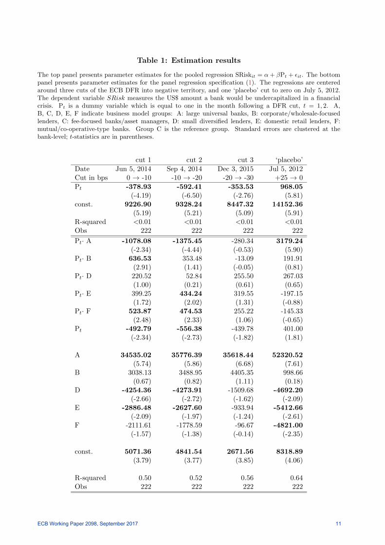
Table 1: Estimation results

The top panel presents parameter estimates for the pooled regression SRiskit = α+ βPt + εit. The bottompanel presents parameter estimates for the panel regression specification (1). The regressions are centeredaround three cuts of the ECB DFR into negative territory, and one ‘placebo’ cut to zero on July 5, 2012.The dependent variable SRisk measures the US$ amount a bank would be undercapitalized in a financialcrisis. Pt is a dummy variable which is equal to one in the month following a DFR cut, t = 1, 2. A,B, C, D, E, F indicate business model groups: A: large universal banks, B: corporate/wholesale-focusedlenders, C: fee-focused banks/asset managers, D: small diversified lenders, E: domestic retail lenders, F:mutual/co-operative-type banks. Group C is the reference group. Standard errors are clustered at thebank-level; t-statistics are in parentheses.

cut 1 cut 2 cut 3 ‘placebo’

Date Jun 5, 2014 Sep 4, 2014 Dec 3, 2015 Jul 5, 2012Cut in bps 0 → -10 -10 → -20 -20 → -30 +25 → 0

Pt -378.93 -592.41 -353.53 968.05(-4.19) (-6.50) (-2.76) (5.81)

const. 9226.90 9328.24 8447.32 14152.36(5.19) (5.21) (5.09) (5.91)

R-squared <0.01 <0.01 <0.01 <0.01Obs 222 222 222 222

Pt· A -1078.08 -1375.45 -280.34 3179.24(-2.34) (-4.44) (-0.53) (5.90)

Pt· B 636.53 353.48 -13.09 191.91(2.91) (1.41) (-0.05) (0.81)

Pt· D 220.52 52.84 255.50 267.03(1.00) (0.21) (0.61) (0.65)

Pt· E 399.25 434.24 319.55 -197.15(1.72) (2.02) (1.31) (-0.88)

Pt· F 523.87 474.53 255.22 -145.33(2.48) (2.33) (1.06) (-0.65)

Pt -492.79 -556.38 -439.78 401.00(-2.34) (-2.73) (-1.82) (1.81)

A 34535.02 35776.39 35618.44 52320.52(5.74) (5.86) (6.68) (7.61)

B 3038.13 3488.95 4405.35 998.66(0.67) (0.82) (1.11) (0.18)

D -4254.36 -4273.91 -1509.68 -4692.20(-2.66) (-2.72) (-1.62) (-2.09)

E -2886.48 -2627.60 -933.94 -5412.66(-2.09) (-1.97) (-1.24) (-2.61)

F -2111.61 -1778.59 -96.67 -4821.00(-1.57) (-1.38) (-0.14) (-2.35)

const. 5071.36 4841.54 2671.56 8318.89(3.79) (3.77) (3.85) (4.06)

R-squared 0.50 0.52 0.56 0.64Obs 222 222 222 222


central bank deposit rates.

Second, rate cuts to negative values lead to different SRisk responses than the July 2012

cut; see the right column in Table 1. For example, SRisk for smaller deposit-taking banks in

groups E and F decreases in 2012 relative to reference group C, and in absolute terms shows

an (insignificant) increase, contrary to what is observed for most later cuts. Large universal

banks (A) are perceived as more risky around the July 2012 cut, possibly reflecting less

dramatic valuation gains from increasing asset prices. Again, the 2012 impact is different

from what is observed for the later cuts. We conclude that cuts to negative rates appear to

be different (‘special’) in terms of their financial stability impact.

References

Acharya, V. and G. Plantin (2017). Monetary easing and financial instability. NYU working paper .

Brownlees, C. T. and R. Engle (2017). SRISK: A conditional capital shortfall measure of systemic

risk. The Review of Financial Studies 30(1), 48–79.

Brunnermeier, M. and Y. Koby (2016). The “reversal interest rate”: An effective lower bound on

monetary policy. Working Paper .

Coeure, B. (2014). Life below zero: Learning about negative policy rates. Speech at the annual din-

ner of the ECB’s market contact group, on 09 September 2014, available at http://www.ecb.int .

Dombret, A. (2017). The ECB’s low-interest-rate policy - a blessing or a curse for the economy,

consumers and banks? Speech delivered at the Sparkassen-Gesprchsforum, Witten, 1 February,

2017 .

Hannoun, H. (2015). Ultra-low or negative interest rates: what they mean for financial stability

and growth. Speech given at the BIS Eurofi High-Level Seminar in Riga, 22 April 2015 .

Heider, F., F. Saidi, and G. Schepens (2017). Life below zero: Bank lending under negative policy

rates. Working paper, available at SSRN: https://ssrn.com/abstract=2788204 .

Lucas, A., J. Schaumburg, and B. Schwaab (2016). Bank business models at zero interest rates.

Tinbergen Institute Discussion Paper 066/IV, 1–56.


Rajan, R. (2013). A step in the dark: unconventional monetary policy after the crisis. BIS Andrew

Crockett Memorial Lecture, 23 June 2013 .

Reinhart, C. M. and K. S. Rogoff (2009). The aftermath of financial crises. American Economic

Review 99 (2), 466–472.

Appendix

The appendix provides two robustness checks. First, we check whether our main empirical results

reported in Table 1 remain qualitatively similar if only the 44 listed banks are used in the analysis.

This is the case. Table A.1 presents the respective testing outcomes. We needed to pool over banks

in groups E and F for data sparsity reasons. Statistical significance is lost in some cases due to

fewer observations in each regression. Table 1, however, remains qualitatively similar.

Second, we implement a formal test (a “placebo test”) of parallel trends. Table A.2 is obtained

by counter-factually assuming that the three DFR cuts occurred one month earlier than they

actually did. With one exception, no interaction effect is significant for the three DFR cuts below

zero. In the one exception, the coefficient is of the opposite sign. Our differential estimates therefore

appear to be associated with the actual DFR cuts.


Table A.1: Estimation results: SRisk subsample of listed banks

The top panel presents parameter estimates for the pooled regression SRiskit = α+ βPt + εit. The bottompanel presents the parameter estimates for the panel regression specification (1). The regressions arecentered around three cuts of the ECB deposit facility rate into negative territory, and one cut to zero inJuly 2012. The dependent variable SRisk measures the US$ amount a bank would be undercapitalizedin a financial crisis. Pt is a dummy variable which is equal to one following a deposit rate cut. A, B, C,D, E indicate business model groups: A: large universal banks, B: corporate/wholesale-focused lenders, C:fee-focused banks/asset managers, D: small diversified lenders, E: domestic retail lenders. Group C is thereference group. T -statistics are in parentheses.

cut 1 cut 2 cut 3 cut +

Date Jun 2014 Sep 2014 Dec 2015 Jul 2012Cut in bps 0 → -10 -10 → -20 -20 → -30 +25 → 0

Pt -726.18 -861.79 -406.79 1236.86(-3.71) (-4.40) (-1.26) (3.34)

const. 13394.86 13347.77 11921.34 20196.89(3.29) (3.25) (3.18) (3.92)

R-squared <0.01 <0.01 <0.01 <0.01Obs 88 88 88 88

Pt· A -1424.90 -1508.04 -98.37 3272.15(-1.65) (-2.52) (-0.09) (2.95)

Pt· B 283.59 -1150.04 -948.5 338.40(0.55) (-0.97) (-0.83) (0.50)

Pt· D 325.42 -76.04 462.44 242.96(0.90) (-0.17) (0.62) (0.34)

Pt· E 422.09 389.25 545.80 -448.29(1.00) (1.01) (1.34) (-1.19)

Pt -661.09 -548.45 -597.00 578.09(-1.91) (-1.61) (-1.49) (1.59)

A 44055.57 45916.72 44081.26 62788.08(3.72) (3.84) (4.12) (4.73)

B 43840.82 41759.09 42220.14 49076.95(1.22) (1.22) (1.30) (1.16)

D -5091.40 -5027.79 -1757.41 -5336.93(-1.87) (-1.87) (-1.08) (-1.42)

E -5027.78 -4769.10 -2525.16 -7551.74(-2.21) (-2.18) (-2.17) (-2.17)

const. 6046.18 5699.90 2993.36 9591.54(2.74) (2.68) (2.58) (2.83)

R-squared 0.56 0.57 0.60 0.65Obs 88 88 88 88


Table A.2: Estimation results: “Placebo” tests at DFR t− 1

Parameter estimates for the panel regression specification (1). The regressions are centered one monthbefore the three ECB DFR cuts into negative territory. The dependent variable SRisk measures the US$amount a bank would be undercapitalized in a financial crisis. Pt is a dummy variable which is equal toone in the second period. A, B, C, D, E, F indicate business model groups: A: large universal banks, B:corporate/wholesale-focused lenders, C: fee-focused banks/asset managers, D: small diversified lenders, E:domestic retail lenders, F: mutual/co-operative-type banks. Group C is the reference group; t-statistics arein parentheses.

Window April/May 2014 July/Aug 2014 Oct/Nov 2015

Pt· A -356.35 -742.22 1545.63(-0.46) (-1.91) (4.02)

Pt· B -293.44 -121.37 58.72(-1.37) (-0.43) (0.35)

Pt· D 146.63 -150.44 404.47(0.62) (-1.19) (1.90)

Pt· E -72.58 33.72 -19.62(-0.45) (0.40) (-0.30)

Pt· F -203.08 10.11 -55.77(-1.42) (0.14) (-0.83)

Pt 240.72 -27.54 42.77(1.74) (-0.41) (0.66)

A 34891.37 36518.61 34072.81(5.94) (6.00) (6.49)

B 3331.57 3610.33 4346.63(0.77) (0.80) (1.14)

D -4400.99 -4123.46 -1914.15(-2.76) (-2.55) (-1.84)

E -2813.89 -2661.32 -914.31(-2.19) (-1.95) (-1.26)

F -1908.52 -1788.70 -40.88(-1.54) (-1.35) (-0.06)

const. 4830.63 4869.08 2628.77(3.92) (3.68) ( 3.96)

R-squared 0.51 0.52 0.54Obs 222 222 222


Acknowledgements Schaumburg thanks the Dutch National Science Foundation (NWO, grant VENI451-15-022) for financial support. The views expressed in this paper are those of the authors and they do not necessarily reflect the views or policies of the European Central Bank.

Federico Nucera LUISS Guido Carli University, Rome, Italy; email: [email protected]

Andre Lucas Vrije Universiteit Amsterdam, Amsterdam, The Netherlands; email: [email protected]

Julia Schaumburg Vrije Universiteit Amsterdam, Amsterdam, The Netherlands; email: [email protected]

Bernd Schwaab European Central Bank, Frankfurt am Main, Germany; email: [email protected]

© European Central Bank, 2017

Postal address 60640 Frankfurt am Main, Germany Telephone +49 69 1344 0Website www.ecb.europa.eu

All rights reserved. Any reproduction, publication and reprint in the form of a different publication, whether printed or produced electronically, in whole or in part, is permitted only with the explicit written authorisation of the ECB or the authors.

This paper can be downloaded without charge from www.ecb.europa.eu, from the Social Science Research Network electronic library or from RePEc: Research Papers in Economics. Information on all of the papers published in the ECB Working Paper Series can be found on the ECB’s website.

ISSN 1725-2806 (pdf) DOI 10.2866/440947 (pdf) ISBN 978-92-899-2820-5 (pdf) EU catalogue No QB-AR-17-110-EN-N (pdf)

mailto:[email protected]




http://www.ecb.europa.eu/

http://www.ecb.europa.eu/

http://ssrn.com/

https://ideas.repec.org/s/ecb/ecbwps.html

http://www.ecb.europa.eu/pub/research/working-papers/html/index.en.html

working paper series - ecb.europa.eu · abstract we study the impact of increasingly negative...

Documents