workforce planning in a lotsizing mail processing … planning in a lotsizing mail processing...

Available online at www.sciencedirect.com

Computers & Operations Research 32 (2005) 3031–3058www.elsevier.com/locate/dsw

Workforce planning in a lotsizing mail processing problem

Joaquim J)udicea ;∗, Pedro Martinsb, Jacinto Nunesc

aDepartamento de Matem�atica, FCT—Universidade de Coimbra, 3000 Coimbra, PortugalbCIO—Centro de Investigac ao Operacional—FC/UL and ISCAC—Instituto Polit�ecnico de Coimbra,

Quinta Agr�'cola—Bencanta, 3040-316 Coimbra, PortugalcCTT—Correios de Portugal, SA, Prac a D. Lu�'s I, 30, 1208-148 Lisboa, Portugal

Available online 9 June 2004

Abstract

The treatment of mail objects in a mail processing centre involves many operations, in particular sorting bydestination. Out of the batching problem that we can identify in such a process, there are also sta4 planningconcerns. In this paper, we analyse a treatment area (registered mail) belonging to a mail processing center,where mail objects are treated in a chain production process. The production quantities and the transferamounts among machines are required to be determined along the daily work period. The objective is tominimize the costs with human resources needed in the process, linked with the lotsizing production plan,by matching sta4 to work requirements. This leads into a lotsizing and workforce problem, for which wepropose an integer programming formulation. A case study of a particular treatment area is also discussed.The formulation is adjusted to the speci6c constraints of this case study and some computational results areincluded, considering average, small and high daily amounts of mail arrived to that particular treatment area.? 2004 Elsevier Ltd. All rights reserved.

Keywords: Workforce scheduling; Batching decision process; Mixed integer programming; Postal service

1. Introduction

This work addresses a particular case of a batching decision process in a mail processing cen-ter (MPC) in the Portuguese Mail Service “CTT—Correios de Portugal, SA”. One of the crucialconcerns of the Sta4 Management Department is the employees’ assignment plan that is needed tocover all the mail Cow in the mail treatment system, where mail-objects are sorted according to theirtype, 6nal destination and duty evaluation.

∗ Corresponding author.E-mail addresses: [email protected] (J. J)udice), [email protected] (P. Martins), [email protected]

(J. Nunes).

0305-0548/$ - see front matter ? 2004 Elsevier Ltd. All rights reserved.doi:10.1016/j.cor.2004.04.011

mailto:[email protected]



3032 J. J�udice et al. / Computers & Operations Research 32 (2005) 3031–3058

The treatment process is made in MPCs placed in the Portuguese territory. Each MPC is dividedinto treatment areas (TAs), according to a speci6c classi6cation of mail-objects: large mail-objects,medium mail-objects, Cats, expressed mail and registered mail. In each TA, the employees’ assign-ment plan is established for a week. In this work, we analyse the year 2001 behaviour of a particularTA, in order to evaluate human resources needs from lower to higher daily mail amounts enteredin that speci6c TA. Those observations are important to plan future manpower needs in that TA.

The treatment process made in each TA involves a prede6ned sequence of treatment units spanningall mail Cow. The mail is treated within 6xed periods of 15 min, and the sequence of consecutiveperiods establishes a partition of the whole planning horizon. Among consecutive periods, the mailtreated is transferred to a subsequent treatment unit through a well-de6ned sequence and accordingto known mail transfer rates. The determination of the amounts treated in each unit and in eachperiod characterizes a batch decision process. All the treatment units require human resources, whichmust be linked with the feasible working shifts in use in the Company.

Therefore, we may identify in the process a single-item multi-level (machine) lotsizing subproblem,characterizing the batching decision process on an acyclic graph de6ned by the 6xed sequence oftreatment units in a single TA, and a shift scheduling subproblem, characterizing the sta4 planningconcerns. It is precisely this last aspect that concentrates the objective of this paper, where workforceoverall costs are required to be minimized.

Like in many applications of operations research, this case also combines known and studiedcentral problems. The 6rst of these subproblems is a multi-stage batch decision problem withoutdirect setup, holding or production costs, but using the same Cow conservation proprieties appearingin multi-level lotsizing problems. Many researchers have devoted attention to the central version ofthis optimization problem (with setup, holding and production costs) (see, e.g. [1–6]). Most of theseworks are motivated by production planning environments, where the multi-level structure is de6nedby a sequence of machines establishing a gozinto structure. There are di4erent types of gozintostructures (see [6]), most of them describing assembly systems. In our problem we do not assembleitems, but we may 6nd in this problem an acyclic gozinto-network of the general type (see [6]),de6ned by the 6xed sequence of treatment units (operations), through which mail-objects (a singleitem) pass through. A general description of various other lotsizing or batch decision related problemscan be found in [7–9]. Formulations for some practical lotsizing based problems are discussed in[10]. Interesting catalogues of selected research are presented in [7,9,11] and various models andoptimization methods are discussed in [10,12–15].The second subproblem is a shift scheduling problem, also known by sta4 planning or workforce

scheduling. It emerges from set covering optimization problems (see, [16]), and comes frequently as-signed to other problems in matching staLng to work requirements, characterizing real applications.Various formulations for shift scheduling problems are compared in [17,18]. Optimization methodsare discussed in [18,19]. A catalogue of selected research is presented in [20] and a review of applica-tions, methods and models has been recently published in [21]. Applications are commonly describedin crew scheduling for bus, rail, air Cight and general transportations planning (see, e.g. [22–27]),ground station personnel scheduling at airports or maintenance teams in daily shift schedules (see,e.g. [28–30]), telecommunication services (telephone operator, telemarketing, customer hotline ser-vice) (see, e.g. [31,32]), public safety (6re, policy, emergency) (see, e.g. [33]), health care (medical,nursery shift scheduling) (see, e.g. [34,35]), and many other cases where shift scheduling planninghas been revealing an important component of ongoing productivity improvement.

J. J�udice et al. / Computers & Operations Research 32 (2005) 3031–3058 3033

Sta4 scheduling has also been applied to the postal sector in [36–38]. The 6rst work [36] addressesa personnel scheduling problem for postal distribution service in the United States postal distributionstations. The authors propose an integer model for this problem, determining daily assignments offull- and part-time employees to di4erent task categories, considering regular and overtime hours.The paper includes some computational results using real data from a typical week in a large postaldistribution station.

The second work [37] addresses a daily personnel scheduling problem to establish weekly tours,involving break time periods and di4erent shift start time periods. The problem considers full- andpart-time employees and satis6es some labour requirements. The authors analyse three problemson the system; the 6rst is concerned with the assignment of days o4 to employees (the days-o4scheduling problem); the second determines an assignment of employees to shifts during the day(the shift scheduling problem); and the third involves the construction of weekly tours (the tourscheduling problem). The problem is motivated by general mail facilities (GMFs), which providefor mail treatment in the US Postal Service and analyses a real application in the Providence, RhodeIsland GMF.

The third work [38] comes in the trend of the second one. The authors expand on the previouswork model and solution techniques and incorporate several new features in their formulation. Theyconsider a linear integer model to solve a weekly tour scheduling problem, determining minimumcost general staLng needs using both full- and part-time employees, respecting labour agreementsand governmental regulations. Di4erent scenarios are examined, including di4erent days o4, vari-able start times and the use of part-time Cexible workers. This work has also been motivated bythe United States Postal Service and applied to the Oklahoma City processing and distributioncentre.

Our problem also involves the determination of an assignment of employees to shifts within adaily working time horizon, where di4erent shifts are considered, involving di4erent durations andstart time periods. In this case, the model is not solved over known workload requirements but itmust cover workloads generated by a batch decision problem running over the same time horizon.Our objective is to determine minimum cost daily workforce needs to treat mail, according to thedaily amounts of mail entered in a single TA.

Many papers that consider shift scheduling as a subproblem have work requirements to be accom-plished, where adequate sta4 coverage is required to be planned (see, e.g., the most of the paperson sta4 scheduling previously mentioned). One of the critics usually pointed to classical lotsizingapproaches, is that it ignores, in most of the cases, that the batch decision structure is only a part ofa larger global management process, turning harder to infer and analyse alternative strategies (see,e.g. [7]). The present combined approach is sensitive to this aspect, relating the two most relevantprocess components, namely the treatment lotsizing scheme of TAs and its sta4 planning concerns.

When looking from the batch decision subproblem perspective, an interesting aspect of the jointsystem establishes that the decision to treat mail in a certain period on a speci6c unit does notdepend on any direct setup cost, like in lotsizing problems, but in the assigned workforce cost,de6ning a kind of an indirect setup cost. This means that the employees’ constraints impose aworkforce upper limit on mail Cow in each unit and in each period, characterizing a capacitatedversion of the multi-level lotsizing subproblem.

In the next section, the company main features and the problem under consideration are de-scribed. A mixed integer formulation for a general treatment area on the MPC scheme is proposed in


Section 3. A speci6c model for a particular treatment area case is described in Section 4, and di4er-ent scenarios solutions to this case study are discussed in Section 5. Some conclusions are presentedin the last section.

2. Company overview and mail processing

2.1. CTT

The company CTT—Correios de Portugal, SA, presents as core business the management andsupport of postal services over the Portuguese territory, as well as international postal servicesbeginning or ending in Portugal.

CTT is divided into the following main job areas: home and company delivery, logistics anddistribution, hybrid mail, 6nancial services and outsourcing services o4ered at the post-oLces all overthe country. To accomplish its purposes, the company has approximately 17 600 employees and ownsnine mail processing centres, 418 mail distribution centres, 1079 post-oLces, 19 000 pillar-boxes andover 4000 vans.

Through the year 2001 over 1370 million postal-objects were processed and nearly 6300 dailypostman routes were made. Money transactions exceeded 17 200 million , which lead the companyto have more than 630 million in revenues with more than 56 million invested.

As a government-owned company, CTT is committed to accomplish quality standard criteria suchas mean time to delivery. The service quality is veri6ed by an independent sector regulator—“ANACOM—Autoridade Nacional de ComunicaPcoes”, which pressures CTT to accomplish with thedelivery.

To plan the mail distribution process, the company divides the Portuguese territory in approxi-mately 418 areas, each having in average 220 km2. Each of these areas has its own mail distributioncentre (MDC), which receives all the mail coming from post-oLces and pillar-boxes inside that areaand sends it to processing centres (MPCs). The MDC also receives mail already treated and havingas 6nal destination an address inside that area. Hence, all the mail received in an MDC is sent to betreated in an MPC. MDCs also receive treated mail coming from an MPC, for distribution purposes.So, postal-objects coming from the MDCs of an area are treated (sorted) at the corresponding MPCand are dispatched from there to its destination MDC.

Postal routes, i.e., the daily journey to deliver mail from door to door, begin at the headquartersof the MDC.

The postal process consists of four main steps, namely collection, sorting by destination, trans-portation and delivery.

Taking into consideration the expected Cow of mail to be treated and the company commitmentwith the quality criteria, it becomes obvious how important it is for this company to plan carefullythe assignment of human resources. Although the MDCs concentrate higher manpower needs, thiswork focus just in the workforce planning in MPCs, where a correct assignment of employees toworkload is also of a great concern, in order to accomplish with the agreed percentage of residualmail at the end of the day, according to the estimated quantity of mail received and to the targetsestablished for quality service.


Mail Processing Center (MPC)

Chain of treatment units





TA1: largemail-objects

TA2: mediummail-objects

TA3: flats

TA4: express mail

TA5: registered mail

MPCmail

in-flow

MPCmail

out-flow

Fig. 1. Scheme of an MPC.

2.2. The MPCs

The main job of an MPC is the mail sorting by type and destination, although it can also work asa point of the course to concentrate and forward mail to other MPCs, where the treatment processtakes place.

The mail classi6cation by type is made on a size basis (small, medium and large) or by specialservice types (express mail and registered mail), being the various types processed in di4erenttreatment areas. Each mail type is entirely processed in the same treatment area, even if it includesdi4erent delivery speeds.

For some mail types and in some MPCs there are automatic processes to sort by destination.Other mail types (e.g. registered mail) are entirely treated by manual processes.

The mail-objects processed have di4erent characteristics. Each MPC has 6ve TAs (designated byTAl, l= 1; : : : ; 5), according to the following features:

• TA1: large mail-objects, including packages and parcels,• TA2: medium mail-objects: essentially periodical publications, like magazines and newspapers,• TA3: Cats: post-cards and letters up to 20 g (0:71 oz),• TA4: express-mail,• TA5: registered mail.

In each TA, mail is treated (sorted and separated) in a chain of specialized treatment units (TUi),characterized by manual and automatic operations. This chain de6nes a productive process, whereone or several units feed other units in a well established sequence. A scheme that characterizes anMPC is presented in Fig. 1.

The MPC operates continuously during all the day, although some TAs are closed during a certainperiod of the day.


TU2

TU3

TU7

0.160

0.740

0. 530

Treatment Area 5 (TA5)

TU9

TU8

TU4

TU6

TU5

TU1

0.0930.540

0.460

0.360

0.250

1.000

1.000

0.280

1.000

0.470

0.007

Arrival /PreparationUnit

TA5 mailin-flow

0.640

0.470

TA5 mailout-flow

DepartureUnit

Fig. 2. Scheme of a TA (TA5).

There is a chain of treatment units (TUi) inside each treatment area, which guarantees mailsorting and separation. Mail objects have to pass through a prede6ned sequence of TUs, where thepercentage of mail-objects that is transferred among each pair of TUs is known. Those transfer ratesare estimated from samples drawn on a regular basis, revealing very small changes along the timeand for this reason being updated in relatively large periods of time. Notice that these transfer ratesdepend mainly on the speci6city of the operations involved in each TU.

We assume no diLculty in the circulation of mail-objects among TUs and all the mail alreadyfully processed goes to a 6nal expedition unit (TUM ) in each TA (M is the total number of TUs).Mail transfer rates among every pair of TUs is de6ned in an (M ×M) matrix P, where pri is the

transfer rate among TUr and TUi, and pri is equal to 0 when there is no connection between thatpair of TUs.

Fig. 2 displays the network describing the sequence of treatment units in TA5 (registered mail).The label in each line connecting two units is their corresponding transfer rate. If two units are notconnected, they do not transfer any mail between them. TU1 (and other non mentioned TUs) receiveall the TA5 incoming mail and TU9 sends all the treated mail to outside. For simplicity, the feedup structure is not represented in the scheme.

The treatment process is made during 6xed periods of 15 min. The complete sequence of con-secutive periods de6nes the global plan horizon. Each TA has its own plan horizon, correspondingto their daily working time duration, which might be as long as 24 h. We also de6ne a 1 h blockas a sequence of four consecutive periods, where each block starts on the hour. Fig. 3 presents agraphical illustration of the various time components used in the treatment process.

Fig. 4 describes the mail Cow scheme, through the periods, between two general treatment unitsTUr and TUi. In each TUi and at each period j, there is an incoming mail quantity which is thesum of the mail directly arrived from outside, the mail at the entrance of TUi and not treated in


1 2 3 4 5 6 7 8 9 10 11 12 13 14 15 16 17 18

1 2 3 4 ...

Plan horizon (no more than 24 hours)

Blocks (1 hour)

Periods (15 minutes)

daily working time

Fig. 3. Graphical illustration of the various time components used in the treatment process.

TUr

TUi

TUr

TUi

(p ri )

Mail-flow from TUr to TUi between sucessive periods

external mail

external mail external mail

external mail

period j-1 period j+1period j

mail maintained in TUi

mail maintained in TUr

mail treated in TUr and transfered to TUi

Fig. 4. Mail-Cow scheme, through the periods, between two general treatment units TUr and TUi. The scheme includesexternal mail entering in each period in both TUs.

the previous periods, and the mail received from preceding units at the end of period j − 1. Thisglobal quantity at the entrance of TUi in the beginning of period j is divided into mail that is treatedduring period j and mail that does not leave the entrance of TUi and waits for its treatment in afuture period in that TU.

Each TA receives their corresponding mail during the daily working time. Mail entered in periodj − 1 is ready to start the treatment process in period j. The mail arriving instants depend on theclosing time of the MDCs and from their distance to the MPC, implying, in general, very smallvariations in those arriving instants. Hence, the amounts of mail arrived during each individual periodis strongly dependent on the global daily mail Cow generated at MDCs and not from the particularbehaviour of those MDCs. Those daily amounts change along the year, with peak weeks in someperiods of the year. Variations on these amounts will be discussed for the particular case studyproposed in this paper.

In order to give the chance to any mail-object to go through on the treatment process, each TUi isnot allowed to receive mail i periods before the end of the plan horizon, where i de6nes a certainnumber of periods and is established by the maximum number of TUs that a mail-object enteredfrom outside to TUi may need to cover until reaching the last TU. Mail arrived to an already closedTU will be treated on the next day.

An upper limit on the quantity of mail that can remain in each TUi at the end of the daily workingtime is assumed. We also impose a standard quality criteria of 99% on the total volume of mailthat must be treated at the end of that same period, i.e. ready to leave the corresponding TA. Theremaining 1% includes mail that is to be treated in the next day.


The Sta4 Management Department intends to plan shift scheduling schemes, to face average andextreme scenarios of daily income mail amounts to each individual TA. The working shifts in use inthe company range between 3 and 8 h shifts, corresponding to 3–8 consecutive 1 h blocks. All theseworking shifts must be included in the overall TA daily working time. Each shift has a 6xed cost peremployee, according to its duration. The purpose of this problem is to minimize the overall workforcesalaries, according to the global assignment of employees to each working shift determined.

In each TA, the employees’ assignment plan is established for each week. So, the problem issolved prior to each week, planning the workforce needs, according to the amounts of mail expectedto be received in that week. This expectation is based on empirical evaluation, based on historicaldata and on typical seasonal behaviour. In fact, we can observe peak weeks, corresponding to lowerand higher income Cow amounts. This behaviour varies according to the type of mail considered ineach particular TA.

In general, workforce availability inside the MPC can be shared between TAs and used forindividual TAs weekly workforce planning. On the other hand, during each week plan established,the employees cannot move from one TA to another. We also assume that any employee can workin any TU inside each TA, at di4erent periods of time. This change between TUs can only occuron the hour, so that in each 1 h block we have a permanent number of employees in each TU. Outof TUM , where we assume no need for manpower assignment, we consider a limit on the numberof employees in each TUi and in each block.

3. A mixed integer linear formulation

In this section, we propose a mixed integer linear formulation for the problem introduced in theprevious section. This formulation combines two sets of constraints, namely lotsizing constraints tocharacterize the batching structure of the problem, and shift scheduling constraints, de6ning its sta4planning structure. As stated before, the objective of this study is concentrated in this last aspect. Westart by presenting all the variables, parameters and constraints for the model. A few explanationsof the main aspects of the formulation are given next.

Parameters:M total number of TUs, (TUM is the last unit in the treatment area)N total number of periods in the time operating interval of the TAH number of 1 h blocksK total number of shiftsck shift k employees individual salary, k = 1; : : : ; Kqij quantity of mail that enters the TA and directly arrives at TUi during period j − 1, i =

1; : : : ; M − 1, j = 1; : : : ; Npri transfer rate of mail-objects from TUr to TUi, r, i = 1; : : : ; M and r �= ibi quantity of mail-objects that a employee can handle in each period in TUi, i= 1; : : : ; M − 1li upper limit on the number of employees at TUi in each 1 h block, i = 1; : : : ; M − 1dk upper limit on the number of employees in shift k, k = 1; : : : ; Kei upper limit on mail quantity allowed to stay in TUi at the end of the process, i=1; : : : ; M−1


akh 1 if shift k covers the hth 1 h block, 0 otherwise, k = 1; : : : ; K; h= 1; : : : ; Hi number of periods that each TUi is closed for mail entrance, before the end of the daily

working time, i = 1; : : : ; M − 1

Variables:xij nonnegative variable, representing the quantity of mail-objects treated in TUi during period j,

i = 1; : : : ; M , j = 1; : : : ; Nsij nonnegative variable, representing the number of mail-objects kept at the end of period j at

TUi, i = 1; : : : ; M , j = 1; : : : ; Nwih integer variable, de6ning the number of employees in TUi during block h; i=1; : : : ; M −1; h=

1; : : : ; Hvk integer variable, de6ning the number of employees assigned to shift k, k = 1; : : : ; K

In this formulation we consider xi0=0 and si0 = 0 (i = 1; : : : ; M); xMj = 0 (j = 1; : : : ; N ) andwMh = 0 (h= 1; : : : ; H); so we can ignore those variables from the model. In order to guarantee thetreatment of the majority of mail-objects that enters the TA, we close each TUi entrance of mailat the (N − i)th period, considering i as the maximum number of TUs that a mail-object enteredfrom outside to TUi may need to cover until reaching TUM . This means that all qij, for i=1; : : : ; Mand j=N − i +1; : : : ; N , should be ignored from the model. The same happens to qMj, because nomail arrives directly to TUM .

Formulation 1:

MinimizeK∑k=1

ckvk (1)

Subject to qij + si; j−1 +M−1∑r=1r �=i

(prixr; j−1) = xij + sij; i = 1; : : : ; M; j = 1; : : : ; N; (2)

siN +M−1∑r=1r �=i

prixrN 6 ei; i = 1; : : : ; M − 1; (3)

sMN +M−1∑r=1

prMxrN ¿ 0:99M−1∑i=1

N−i∑j=1

qij (4)

xij6 biwih; i = 1; : : : ; M − 1; j = 1; : : : ; N; h= �j=4�; (5)

wih6 li; i = 1; : : : ; M − 1; h= 1; : : : ; H; (6)

M−1∑i=1

wih =K∑k=1

akhvk ; h= 1; : : : ; H; (7)

vk6dk; k = 1; : : : ; K; (8)


xij¿ 0; i = 1; : : : ; M; j = 1; : : : ; N; (9a)

sij¿ 0; i = 1; : : : ; M; j = 1; : : : ; N; (9b)

wih ∈N0; i = 1; : : : ; M − 1; h= 1; : : : ; H; (10a)

vk ∈N0; k = 1; : : : ; K: (10b)

Constraints (2) are the Cow conservation constraints in each TUi and in each period j, and theyestablish the equilibrium between the incoming and the outgoing mail quantity in the mentionedTU in period j. The incoming mail is de6ned as the sum of the mail arrived during the (j − 1)thperiod (qij), the mail at the entrance of TUi and not treated in the previous periods (si; j−1), and

the mail received from preceding units at the end of period j− 1(∑M

r=1 r �=i prixr; j=1

). This quantity

at the entrance of TUi in the beginning of period j must be equal to the mail treated in periodj (xij) plus the mail that does not leave the entrance of TUi (sij) and waits to be treated in afuture period in TUi. Constraints (3) impose an upper limit on the number of mail-objects allowedto stay in each TU at the end of the process. The (prixrN ) terms represent mail treated in precedingTUs, which are transferred to TUi at the end of the N th period. Inequality (4) guarantees that99% of the overall mail that enters in TA is assembled in the 6nal TUi at the end of the process.Notice that xMj = 0 (j = 1; : : : ; N ), so the 6nal arrival TU simply accumulates (almost) all themail Cow and it does not require any employees. These three sets of constraints characterize themulti-level lotsizing structure of the problem. On the other hand, inequalities (6)–(8) describe theshift scheduling subproblem. Considering this separation, inequalities (5) can be seen as couplingconstraints, relating the treatment variables (xij) with the sta4 slot variables (wih). They guaranteea suLcient number of employees to cover the mail treatment in each period in TUi. Constraints(6) and (8) impose upper limits to the number of employees in each TUi and in each shift k,respectively. We relate these two sets of variables (wih and vk) in constraints (7), guaranteeing theemployees assignment among shifts and their corresponding 1 h blocks, according to the variousshift intervals allowed. The objective is to minimize the overall workforce cost in this TA, whichis stated in the objective function (1).

We consider variables xij and sij as nonnegative, although representing nondivisible units (mail-objects). This option simpli6es the problem and represents a negligible lost to the correct descriptionof the problem, due to the discrepancy of a unit in the total amount of mail treated. The othervariables represent employees and have to be de6ned as integer variables.

An interesting aspect of this model is characterized by the coupling constraints (7). Contraryto a sta4 decision problem, we do not simply impose a cover from a selection of shifts over thetotal workforce in each one hour block, de6ned by the inequalities

∑M−1i=1 wih6

∑Kk=1 akhvk to each

h∈ {1; : : : ; H}. Instead, we further demand the two quantities in each term to be equal, which impliesEqs. (7). The solutions to be dropped (those verifying

∑M−1i=1 wih ¡

∑Kk=1 akhvk), are concerned with

cases where we have a smaller number of employees assigned to TUs than those assigned to the shiftscovering a certain block h. We can show that any of those solutions can be substituted by anotherfeasible solution, obtained from the previous one by just increasing the values of the variables wih

until we reach the equality de6ned by constraint (7). Both solutions have the same objective functionvalue. By using the equality constraints a signi6cant number of dominated solutions are dropped from


the model. This reduction is especially important in the linear relaxation version of the model, whichmay contribute to the eLciency of the optimization process, when LP relaxation techniques are usedto solve the problem. This is highlighted in Chapter 5 which reports computational experience withthis type of models.

An important aspect on the mentioned transformation is related with the assurance of its feasibility,according to the upper-bound limit imposed to the number of employees in each TU, de6ned inconstraints (6). In this case, by adding constraints (6) to every i∈ {1; : : : ; M − 1}, we obtain thefollowing 6xed upper limit

∑M−1i=1 wih6

∑M−1i=1 li=L, which is the same in every 1 h block. Hence∑K

k=1 akhvk6L, so for two di4erent blocks h1 and h2, the upper bound de6ned in constraints (6)do not impose a positive gap between

∑M−1i=1 wih1 and

∑Kk=1 akh1vk . This allows at the same time

an equality between the same two terms in block h2, as both∑K

k=1 akh1vk and∑K

k=1 akh2vk havethe same upper bound (L). This means that the upper limit constraints (6) neither exclude therepresentative valid solutions from the model, nor turn the problem to be infeasible.

4. A case study: the treatment area TA5

The formulation proposed in Section 3 characterizes a general operating structure of a TA. In thissection, we concentrate our attention in a speci6c treatment area, namely TA5, in which registeredmail is treated. Next, some particular features related with this area are included, which follow fromthe network presented in Fig. 2. The daily working time in this particular case is de6ned from 17:00to 04:00. Table 1 includes the corresponding working shifts.

Two distinct time intervals are considered in the overall daily working time. The 6rst starts at17:00 and ends at 23:00, while the second one starts immediately after the end of the 6rst and endsat 4:00. We refer to both time intervals as working time 1 and 2, respectively. Some characteristicsof both periods are stated below.

Time interval 1—from 17:00 to 23:00: In this time interval, regional mail (addressed to the sameMPC area) arrives at TA5 together with mail to other MPC areas (inter-regional mail). So it is

Table 1Feasible working shifts in TA5, ordered sequentially

Working shifts

No. 3 h No. 4 h No. 5 h No. 6 h No. 7 h No. 8 h

1 [17:00–20:00] 10 [17:00–21:00] 18 [17:00–22:00] 25 [17:00–23:00] 31 [17:00–24:00] 36 [17:00–01:00]2 [18:00–21:00] 11 [18:00–22:00] 19 [18:00–23:00] 26 [18:00–24:00] 32 [18:00–01:00] 37 [18:00–02:00]3 [19:00–22:00] 12 [19:00–23:00] 20 [19:00–24:00] 27 [19:00–01:00] 33 [19:00–02:00] 38 [19:00–03:00]4 [20:00–23:00] 13 [20:00–24:00] 21 [20:00–01:00] 28 [20:00–02:00] 34 [20:00–03:00] 39 [20:00–04:00]5 [21:00–24:00] 14 [21:00–01:00] 22 [21:00–02:00] 29 [21:00–03:00] 35 [21:00–04:00]6 [22:00–01:00] 15 [22:00–02:00] 23 [22:00–03:00] 30 [22:00–04:00]7 [23:00–02:00] 16 [23:00–03:00] 24 [23:00–04:00]8 [00:00–03:00] 17 [00:00–04:00]9 [01:00–04:00]


necessary to separate both types of mail and to sort them by destination. There are two demands inthe treatment of the mail:

(i) TU7 simply treats inter-regional mail, which has to be ready for expedition before 23:00. Thismeans that inter-regional mail (which comes from TU7) should be ready in TU9 before theend of the 6rst time interval. The regional mail processed during this time interval is kept atTU8. Although there are two di4erent items (regional and inter-regional mail) in this problem,we consider it as a single-item case.

(ii) Regional mail must be treated before 04:00 and should be in TU9 before that time.

Time interval 2—from 23:00 to 04:00: In this period only regional mail (addressed to the sameMPC area) arrives at TA5. This mail does not require any kind of preparation, hence node 1 iseliminated from the network.

Therefore, the original matrix P = [pri]r; i=1; :::;M is splitted into two matrices P1 = [p1ri]r; i=1; :::;Mand P2=[p2ri]r; i=1; :::;M , where M is the number of TUs and P1 and P2 are concerned with the timeintervals 1 and 2, respectively.

TUM−2 and TUM−1 can share their human resources availability, so we consider their manpowerassignment in conjunction. We simply demand mail to be kept separated (regional and inter-regional),while treated by the same team.

Considering these further characteristics, the following mixed integer programming model can beassociated to the treatment area TA5, where N1 represents the number of periods until 23:00.

Formulation 2:

MinimizeK∑k=1

ckvk (1)

Subject to qij + sij−1 +M−1∑r=1r �=i

(p1rixrj−1) = xij + sij; i = 1; : : : ; M; j = 1; : : : ; N1; (11a)

qij + sij−1 +M−1∑r=1r �=i

(p2rixrj−1)=xij+ sij; i=1; : : : ; M; j = N1+1; : : : ; N; (11b)

siN1 +M−1∑r=1r �=i

p1rixrN16 0:01

N1−i∑j=1

qij +N1∑j=1

M−1∑r=1r �=i

p1rixrj

;

i = 1; : : : ; M − 2; (12a)

siN +M−1∑r=1r �=i

p2rixrN 6 0:01

N−i∑j=1

qij +N1∑j=1

M−1∑r=1r �=i

p1rixrj +N∑

j=N1+1

M−1∑r=1r �=i

P2rixrj

;

i = 1; : : : ; M − 1; (12b)


M∑i=M−1

siN1 +

M−1∑r=1r �=i

p1rixrN1

¿ 0:99

M−1∑i=1

N1−i∑j=1

qij; (13a)

sMN

M−1∑r=1r �=i

P2rMxrN ¿ 0:99M−1∑i=1

N−i∑j=1

qij; (13b)

xij6 biwih; i = 1; : : : ; M − 3; j = 1; : : : ; N; h= �j=4�; (14a)

xM−2j + xM−1j6 bM−2wM−2h; j = 1; : : : ; N; h= �j=4�; (14b)

wih6 li; i = 1; : : : ; M − 2; h= 1; : : : ; H; (6)

M−2∑i=1

wih =K∑k=1

akhvk ; h= 1; : : : ; H; (7)

xij¿ 0; i = 1; : : : ; M; j = 1; : : : ; N; (9a)

sij¿ 0; i = 1; : : : ; M; j = 1; : : : ; N; (9b)

wih ∈N0; i = 1; : : : ; M − 2; h= 1; : : : ; H; (10a)

vk ∈N0; k = 1; : : : ; K: (10b)

As before, variables xi0, si0 (i=1; : : : ; M) and xM;j (j=1; : : : ; N ) and parameters qij (i=1; : : : ; M ;j = N − i + 1; : : : ; N ) can be ignored from the model. Furthermore, it follows from the networkpresented in Fig. 2 that there are M =9 TU units and 1=4, 4=3, 2=3=5=6=2, 7=8=1.Remember that TU9 does not receive mail from outside.

This formulation di4ers from the previous one in some constraints, that are discussed next. Thosedi4erences are directly related with the mentioned features of the treatment area TA5. In the setof Cow conservation constraints (11a) and (11b), matrices P1 and P2 de6ne the new transfer ratenetwork structure in both time intervals. Constraints (12a) and (12b) substitute inequalities (3),which de6ne upper limits to the end process residual number of mail-objects that can be left in eachTU and are directly dependent on the global volume of mail arrived to each of those TUs (no morethan 1% of this quantity), in both end time periods, N1 and N , respectively. The new constraintsestablish a non constant upper limit on the amount of mail allowed to remain in each TU, di4eringfrom inequalities (3) proposed for the general case. Out of the 99% of mail to be treated at the endof the process and de6ned by the constraint (13b), we must guarantee that all the mail entered untilthe (N1 − i)th period should be at TUM−1 (regional mail) and at TUM (inter-regional mail) untilthe end of period N1. This is de6ned in the constraint (13a), allowing a 1% tolerance of unsentinter-regional mail plus non accumulated regional mail at TUM−1, at the end of the N1th period.Notice that this 1% tolerance of undelivered mail is established by the standard quality criteria, whilethe previous 1% TUs residual mail tolerance is an internal organizational criteria, so both conceptscannot be self-substituted. The lower limit on the number of employees (wih) imposed by the amountof mail treated (xij) is the same as before. We consider apart the TUM−2 and TUM−1 cases, where


both units amount of mail treated is covered by the number of employees assigned to TUM−2. Thisleads into constraints (14b). Notice that there is no need of human resources assigned to TUM . Asmentioned at the end of Section 2.2, workforce availability inside an MPC can be shared amongTAs and used for individual TAs weekly workforce planning. TA5 is not very demanding in humanresources needs, when compared with other TAs. For this reason, no upper limits to the number ofemployees in each shift are assumed, hence inequalities (8) have be deleted from the present model.

5. Computational experiments to the case study

Consider the case study presented in the previous section and based in Fig. 2 treatment scheme.Furthermore, let the daily working time of TA5 be the one settled before, from 17:00 to 4:00. Hence,the following parameters are set in Formulation 2:

(i) M = 9—number of TUs,N = 44—number of periods (N1 = 24),H = 11—there are 11 blocks in the 17:00 to 04:00 time interval,K = 39—number of working shifts of 3–8 h, as de6ned in Table 1.

(ii) Costs for each working shift of 3, 4, 5, 6, 7 and 8 h: (ck ; k = 1; : : : ; K)

Shifts duration (h) 3 4 5 6 7 8

Cost ( ) 18.66 24.88 31.10 37.32 43.54 49.76

All the costs are proportional to 6.22 , de6ning the hourly cost of work. Nonproportionalcosts, according to shifts duration, do not impose any further diLculties to the problem.

(iii) Matrices P1 and P2 are de6ned in Appendix A, where p1ri is the mail-Cow transfer rate fromTUr to TUi (r; i=1; : : : ; M) in the 17:00–23:00 time interval, and p2ri is the mail-Cow transferrate from TUr to TUi (r; i = 1; : : : ; M) in the 23:00–04:00 time interval.

(iv) The parameters qij (i=1; : : : ; M − 1, j=1; : : : ; N ) are de6ned in Appendix A, representing thenumber of mail-objects arrived directly to each TU per period.

(v) We also consider processing speed rate values, de6ned by bi (i = 1; : : : ; M) parameters. Theseare presented in the following table, by mail-objects/man per period:

TU 1 2 3 4 5 6 7 and 8

Mail-objects/man 1500 250 280 313 313 25 350

We assume that no more than 15 employees can simultaneously be in the same TU, so li = 15for i= 1; : : : ; M . As stated before, we have ignored the upper limit on the number of employees onthe same working shift, which means that constraints (8) have been dropped from the model.

We have used the ILOG/CPLEX 7.0 package LP and mixed integer (MIP) solver to process themixed integer linear programming Formulation 2 with all the mentioned parameters. Thebranch-and-cut version of the MIP solver has been chosen, which allows the generation of


general feasible cuts, provided by the software. The optimization model has been run in aPentium III 800 MHz processor machine.

Next some scenarios are analysed, showing the problem sensitivity to some of its inputparameters. These changes focus on the daily amount of mail arrived to TA5 and on the qual-ity criteria level. As mentioned in Section 2.2, the mail arriving instants to this area, and also to theother ones, depend on the closing time of the MDCs and on their distance to the MPC, implying, ingeneral, very small variations in those arriving instants. Hence, the amounts of mail arrived duringeach individual period are strongly dependent on the global daily mail Cow generated at MDCsand not to the particular behaviour of those MDCs. Those daily amounts change along the year,with peak weeks in some periods of the year. In this paper, year 2001 daily income mail-Cow isanalysed for TA5, in order to evaluate human resources needs from lower to higher amounts ofmail entered in that speci6c TA. Those observations are important to plan future manpower needsat TA5.

Consider the total amount of mail arrived to TA5 in a speci6c day, de6ned by Q=∑M−1

i=1

∑N−ij=1 qij.

Then, for the year 2001, the 251 daily observed Q values conduct to the following statistical pa-rameters: Wx = 46 925, s = 13 715:923, skewness = −0:29 (with std. error of skewness = 0.148)and kurtosis = 0.458 (with std. error of kurtosis = 0.148). Although both quotients (skewness andkurtosis divided by their respective std. errors) fall between −2 and 2, the Kolmogorov–Smirnov(with Lillierfors correction) goodness-of-6t test gives no evidence that the sample comes from theNormal distribution with the estimated sample parameters, presenting a p-value equal to 0.002. Weused the SPSS statistical software, version 11.0 (see [40]).

Based on these observations, the following four points are to be addressed next:

(i) the average case (Q = 46 925), including some aspects related with Formulation 2 resolutionand some changes on the model parameters;

(ii) a comparison between small, average and high mail amount cases, considering Q=36 709 (6rstquartile), Q = 46 925 and Q = 55 006 (third quartile), respectively;

(iii) the analysis of the weeks with small and high average amounts of mail arrived, consideringthe median observation in those weeks, with Q = 25 947 and Q = 69 039, respectively;

(iv) the analysis of the weeks with highest and shortest di4erences between the maximum and themedian observations.

Due to some privacy options of the Company, the comparison with the practical solutions in useare simply provided for the aggregated average case.

The qij parameters table, presented in Appendix A, de6nes the average case income mail quantitiesarrived per period, so for Q = 46 925. For di4erent Q values, the qij quantities are proportional tothose presented in the mentioned table.

(i) Average case: The linear relaxation optimal solution value of Formulation 2 de6nes a lowerbound equal to 610.36 , and was obtained after 0:28 s of CPU time.The MIP solver of CPLEX 7.0 was unable to reach optimality after 12 h of running time. Neverthe-

less, some interesting feasible solutions have been obtained during the branch-and-bound execution.The best lower and upper bounds found at the end of this experience are 638.69 and 646.88 ,respectively. Hence there is a duality gap of 1.27%. In the 6rst node of the branch-and-bound tree,the MIP solver strength the model with 84 Gomory fractional cuts and four MIR cuts, leading thelower bound to 615.05 . After some experiences on node and variable selection strategies of the


0

5

10

15

20

25

num

ber

of e

mpl

oyee

s

17:00-18:00 18:00-19:00 19:00-20:00 20:00-21:00 21:00-22:00 22:00-23:00 23:00-0:00 0:00-1:00 1:00-2:00 2:00-3:00 3:00-4:00

Fig. 5. Number of employees determined per block.

MIP solver, we have chosen to use the best-bound search strategy for node selection and the variableselection based on pseudo-costs (see [39]).

In this case, the normal daily treatment process of this TA is guaranteed by a 104 h workforcesolution, corresponding to a 646.88 daily cost. The 1.27% duality gap simply corresponds to 1 hworkforce, that is, either the best feasible solution is optimal or there is an optimal solution requiringone less hour.

We have also tried to solve the problem starting the branch-and-bound method fromFormulation 2 with constraints (7) de6ned as less or equal inequalities, characterizing the shiftscovering over the hourly assignment of employees to TUs. In this case, we reached the same 104 hfeasible solution, although the lower bound obtained after the same 12 h of running time was equalto 636.41 , de6ning a 1.62% duality gap, that is superior to the one obtained in the previous case.

The best feasible solution found is presented in Table 10 in Appendix B, which presents thenumber of employees determined per block and assigned to each TU: variables wih values.Fig. 5 shows the total number of employees per block, according to the 104 h solution found.Fig. 6 presents the amount of mail-objects in the system and not yet treated (line) per period

j (j=1; : : : ; 44), de6ned by the di4erence between the total amount entered before period j and thequantity already arrived at TU9. The 6gure also shows the total amounts entered per period j (stars)(arrived during the (j − 1)th period).We cannot establish a fair comparison between both charts, because the speed rate (in mail-objects

per period) among TUs is di4erent. In any case, if we try to lean Fig. 6 against Fig. 5, it givesan idea of how workforce adapts to the mail amount being treated, per block. That comparisonshows, for instance, that the 12 employees assigned to the 3 h shift (1:00–4:00), which allows fora signi6cant decrease of mail-objects in the (1:00–2:00) block, may reCect some spare capacity inmanpower usage in the time interval from 2:00 to 4:00. This spare capacity might be appropriatelyused if an augmented amount of mail (namely regional mail) arrives to this TA. Notice that ourminimum duration shifts are three hours time intervals.

Table 2 presents the number of employees determined per shift type, and described by the solutionvalues of the variables vk . No employees have been assigned to the remaining shifts that are notincluded in this table.

We may think in many alternative scenarios, still centred in the average arrived amount case(Q=46 925). Some of these alternative cases are discussed in the next paragraphs, obtained throughappropriate changes in some parameters.


5000

10000

15000

20000

25000

30000

35000

0

mai

l-ob

ject

s

17:00-18:00 18:00-19:00 19:00-20:00 20:00-21:00 21:00-22:00 22:00-23:00 23:00-0:00 0:00-1:00 1:00-2:00 2:00-3:00 3:00-4:00 blocks

periods1 2 3 4 5 6 7 8 9 10 11 12 13 14 15 16 17 18 19 20 21 22 23 24 25 26 27 28 29 30 31 32 33 34 35 36 37 38 39 40 41 42 43 44

Fig. 6. Amount of mail-objects in the system and not yet treated (line) per period j, and the total amounts entered perperiod j (stars) (arrived during the (j − 1)th period), for j = 1; : : : ; 44.

Table 2Number of employees determined per shift type: variables vk solution values

Shifts Number of employees

18:00–21:00 118:00–22:00 219:00–22:00 1320:00–23:00 601:00–04:00 12

It can be showed that for the same amount of mail-objects arrived (Q = 46 925), the 104 hworkforce can treat up to 46 742 mail-objects, corresponding to 99.61% of the total amount entered.This means that the proposed workforce can go beyond the 99% standard for the quality criteria.Notice that the previous reported best feasible solution, described in Table 10 in Appendix B, onlytreat 46 456 mail-objects, corresponding to 99% of the total amount. The 99.61% solution has beenobtained from a changed version of Formulation 2. The new model involves the maximization ofthe nonnegative variable �, representing the standard quality criteria, also appearing in constraints(13a) and (13b). The model includes the following additional constraint:

K∑k=1

�kvk = 104 (15)

to force the use of only 104 h of workforce (�k is the time duration, in hours, of shift k).In a di4erent perspective, we also looked for the maximum increase on the total amount of mail

that TA5 can receive, keeping the same 99% quality criteria and forcing again for a 104 h of man-power usage. This case involves a di4erent changed version of Formulation 2, which includes a


Table 3MIP solver information related with the three quality criteria scenarios: 97%, 95% and 90%

Quality criteria (%) Lower bound ( ) Upper bound Duality gap (%)

97 617.25 628:25 = 101 h 1.75195 609.55 622:04 = 100 h 2.00890 591.85 603:38 = 97 h 1.911

new nonnegative variable , de6ning the proportional increase in the previous amount of 46 925mail-objects. So the new formulation involves the maximization of , subject to Formulation 2constraints, added by equality (15) and substituting all the parameters qij by qij , in constraints(11a)–(13b). After 12 h of the branch-and-bound execution, the best feasible solution found was = 1:0044, with an upper bound de6ned by = 1:0258. This means that we can treat at least47 131 mail-objects with the same workforce resources with no damage to the service quality stan-dards, corresponding to more 206 mail-objects when compared with the initial case (for proportionalincreases). This increase can not exceed 1210 mail-objects, considering the upper bound value ob-tained. Remember that it is assumed that an increase on the daily mail amount entered is establishedby proportional increases in each period mail amounts arrived, according to the qij values presentedin Appendix A.Another interesting aspect is related with the 99% standard quality criteria on the total amount of

mail treated, and the 1% of mail that is allowed to stay in each TU and treated in the next day.As mentioned in Section 2.1, an independent sector regulator follows the time series movement ofdelayed mail. Those limits are agreed with the Company and are frequently a matter of discussion.At this point, we may discuss two scenarios: the 100% quality criteria; and relaxed standard qualitycriteria’s. We start by the 6rst scenario.

From an optimizer perspective, these tolerances seem to be an imperfection of the system, whichshould not be assumed by the model. From the manager perspective, these tolerance limits havelong been studied, and reCect a good compromise between an admissible negligible failure andthe additional workforce cost needed to accomplish this failure. If we try to answer the optimizerexpectations by solving Formulation 2 with 100% quality criteria and 0% mail left on TUs (providingthe appropriate changes in constraints (12a), (12b), (13a) and (13b)), we obtain (again after 12 hof the branch-and-bound execution) a lower bound equal to 676.43 and an upper bound equalto 690.46 . This means that the optimal solution to that speci6c problem involves between 109and 111 workforce hours. So to close this residual volume of nontreated mail, we must spend atleast more 5 h, representing an increase on the overall manpower e4ort. This solution is interestingto compare with the previous reported case, which showed that we are able to treat 99.61% ofthe global amount entered using only the 104 h workforce. So the mentioned 6ve additional hoursrequired to meet the 100% case reCect only 0.39% (183 mail-objects), when keeping the same globalamount entered (46 925 mail-objects).

For the relaxed scenarios, we have considered the following standard quality criteria parameters:97%, 95% and 90%, keeping the 1% residual mail tolerance at TUs and all the other initial parame-ters. In this case, the changes are only present in constraints (13a) and (13b). After 12 h of runningtime, the MIP solver gave the solutions presented in Table 3.


111

104

101100

97

109

103

10098

96

85

90

95

100

105

110

115

90% 95% 97% 99% 100%

Upper Bound

Lower Bound

num

ber

of e

mpl

oyee

s

Fig. 7. Lower and upper bound number of employees determined to the 6ve quality criteria scenarios: 90%, 95%, 97%,99% and 100%.

These three scenarios and the previous 99% and 100% cases are compared in Fig. 7. All thecases are de6ned in workforce hours, including the lower bound transformed values, which are ob-tained from the expression �(lower bound)=6:22� (remember that the hourly cost of work is equal to6.22 ), de6ning a lower limit on manpower usage.

Fig. 7 shows that, when placed at the 99% case, the additional workforce e4ort needed to increasethe quality criteria is much superior than the bene6t obtained from relaxing that same quality criteria.In fact, comparing only the upper bound values, the 1% quality criteria increase over the 99% caserequires seven additional workforce hours, which coincides with the manpower spared from relaxingthe quality criteria to 90%. This subject is a frequent theme of discussion in the Company, to whichthe previous analysis indicate that a decrease in the delivery quality standards may not correspondto a signi6cant decrease in manpower usage.

In order to compare with the practice in this TA5, we applied to the MPC manager for a practicalworkforce solution to the 46 925 mail-objects case, keeping all the parameters initially introduced.This MPC has recently been installed and the current manager has been adapting its workforceavailability to the various TAs, making successive experiences on employees’ local changes. Forthe average case considered to TA5, his proposal corresponds to a 112 h workforce, representing696.64 , using the same kind of 3–8 h shifts and verifying the same quality criteria described andused to build Formulation 2. This represents a gap of 7.14%, when compared with the best solutionproposed in this paper.

This comparison shows not only the great interest of the optimization formulation presented inthis paper but also the con6rmation that the solution proposed by the manager to this TA5 was notfar from the best he could a4ord to, although the 104 h solution shows that he could have gonefurther.

In a di4erent perspective, it is also interesting to analyse the case where only 8 h working shiftsare in operation. By adapting Formulation 2 to that particular situation, we obtain an optimal solutionof 945.44 on daily salaries, using 152 h of total workforce. This means that by using the 3–8 hshifts solutions, we can reduce signi6cantly the human resources needs in this particular TA.

(ii) Comparison between small, average and high amount cases: In this point, we analyse theaverage case: Q = 46 925, and also small and high daily amounts of mail-objects entered at TA5.The small and high amount cases are the 6rst and the third quartiles, namely Q=36 709 and 55 006,


Table 4Workforce solutions per block determined to the Q1, WQ and Q3 mail arrival scenarios

Blocks 17:00–18:00

18:00–19:00

19:00–20:00

20:00–21:00

21:00–22:00

22:00–23:00

23:00–0.00

0:00–1:00

1:00–2:00

2:00–3:00

3:00–4:00

Total

Q1 0 2 11 17 16 7 0 0 10 10 10 83WQ 0 3 16 22 21 6 0 0 12 12 12 104Q3 1 1 15 25 24 11 0 0 15 15 15 122

Table 5MIP solver information related with the three mail arrival scenarios: Q1, WQ and Q3

Amounts entered Lower bound ( ) Upper bound Duality gap (%)

Q1 501.80 516:30 = 83 h 2.89WQ 638.69 646:88 = 104 h 1.27Q3 739.52 758:88 = 122 h 2.55

respectively. We designate the three mentioned cases by WQ = 46 925, Q1 = 36 709 and Q3 = 55 006,respectively.

Table 4 presents the number of employees per block in the best feasible solution obtained by theMIP solver, after 12 h of running time. The standard quality criterion has been kept at a 99% level.Like the WQ case, the other two quantities analysed (Q1 and Q3) require only 3 and 4 h shifts.In Table 5, the lower and upper bound limits obtained after 12 h of the branch-and-bound execu-

tion, and the associated duality gaps, are reported.These results show that a workforce ranging between 83 and 122 h can answer 50% of the 251

observations of daily mail income amounts. This means that the 122 h workforce solution is suLcientto treat 75% of the mentioned 251 observations, when the quality criteria is established at a 99%standard. This result may introduce a new discussion, that is, how far could we go, answeringto the 251 daily observations, with the same 122 h of workforce, if the quality criteria standardis decreased? To answer this question, we have analysed unitary decreases on the quality criteriavalue, from 99% to 88%, where the objective is to determine the maximum amount of mail-objectsallowed to enter to TA5 and treated, at the quality standard established, by a 122 h workforce. Thisanalysis is similar to a previous one, proposed in point (i). It also involves a changed version ofFormulation 2, which includes the same non-negative variable , de6ning the proportional increase inthe 55 006 amount of mail-objects. The modi6ed formulation involves the maximization of , subjectto Formulation 2 constraints, together with equation

∑Kk=1 �kvk = 122 (�k is the time duration, in

hours, of shift k) and substituting all the parameters qij by qij , in constraints (11a)–(13b). Table 6presents the best feasible solutions found to each of the approaches, from 99% to 88% cases, after12 h of the branch-and-bound execution. The accomplishment columns represent the percentage ofaccomplishment achieved over the 251 daily observations. To each daily amount observation Q, thementioned accomplishment is considered at the quality criteria level (!) established, so consideringthat Q! mail-objects are treated.


Table 6MIP solver information related with the twelve quality criteria standards: 99–88%, imposing the use of 122 h of workforce.Mail-objects (m-o) are rounded to the closest integer value

Workforce=122 h, qualitycriteria (!) (%)

Lower bound Accom-plishment(%)

Upper bound Accom-plishment(%)

Dualitygap (%)

99 ¿ 1:008 = 55466 m-o 76 6 1:018 = 55996 m-o 77 0.9898 ¿ 1:014 = 55776 m-o 77 6 1:059 = 58251 m-o 83 4.2597 ¿ 1:041 = 57249 m-o 79 6 1:083 = 59595 m-o 86 3.8896 ¿ 1:061 = 58361 m-o 83 6 1:106 = 60837 m-o 89 4.0795 ¿ 1:092 = 60064 m-o 86 6 1:126 = 61941 m-o 90 3.0294 ¿ 1:101 = 60562 m-o 88 6 1:142 = 62817 m-o 91 3.5993 ¿ 1:118 = 61497 m-o 90 6 1:158 = 63697 m-o 92 3.4592 ¿ 1:153 = 63447 m-o 91 6 1:180 = 64907 m-o 93 2.2991 ¿ 1:176 = 64687 m-o 93 6 1:194 = 65677 m-o 94 1.5190 ¿ 1:194 = 65695 m-o 94 6 1:210 = 66557 m-o 94 1.3289 ¿ 1:212 = 66667 m-o 94 6 1:224 = 67327 m-o 95 0.9888 ¿ 1:224 = 67327 m-o 95 6 1:242 = 68317 m-o 95 1.45

9291

9089

86

83

9088

86

83

7977 77

95 9594 94

93

76

95 94 9493

91

75

80

85

90

95

100

88 89 90 91 92 93 94 95 96 97 98 99

Upper Bound

Lower Bound

quality criteria (%)

acco

mpl

ishm

ent %

Fig. 8. Lower and upper bound values of the accomplishment to each quality criteria level, ranging from 99% to 88%,with a 6xed workforce of 122 h.

Fig. 8 presents the lower and upper bound values of the accomplishment achieved according tounitary variations in the quality criteria level, considering the results in Table 6.

As expected, when the quality criteria level is allowed to be decreased, the 122 h of workforce aresuLcient to answer to a higher number of days, in the 251 universe. Namely, for a quality criterialevel of 99%, the 122 workforce hours are suLcient to answer to at least 76% of the days, whileif that quality standard is allowed to be relaxed to 93%, then the same workforce can answer upto 90% of the days. If only 5% of the days are allowed to fail with the quality criteria established,than this standard must be relaxed to 88%, still using the same workforce.


Table 7MIP solver information related with the two scenarios: Q− and Q+

Daily mail amounts Lower bound Upper bound Duality gap (%)

Q− = 25 947 376:50 → 61 h 379:42 = 61 h 0.77Q+ = 69 039 914:82 → 147 h 933:00 = 150 h 1.95

We recall that the 122 workforce hours solution has been suggested to answer the Q3 amount ofmail case, being suLcient to guarantees a 99% quality criteria on 75% of the days. The previousresult shows that we can go further, establishing that the same manpower level can answer at least76% of the days, still keeping the same quality criteria standard.

(iii) Weeks with small and high average amounts of mail arrived: The previous analyses arerelated with daily income mail amounts, based on the 251 daily observations of the year 2001. Asmentioned in Section 2.2, in practice, TA5 employees’ assignment plan is established for each week,according to the amounts of mail expected to be received during that week. In this point, and alsoin the next one, year 2001 data observations are going to be analysed again, but this time lookingfor its weekly behaviour.

In those data values, the median observation in the weeks with smaller and higher average mailincome amounts are Q− = 25 947 and Q+ = 69 039 mail-objects, respectively. These two peakweeks may be seen as low and hard workforce weeks in human resources needs. The low weekcase can be observed in August during the typical vacations period, when most Public Institu-tions are closed. The high week peak occurs in December and may be related with Christmastime and with the proximity of the end of the year. Remember that TA5 only treats registeredmail.

In Table 7, the lower and upper bound limits obtained after 12 h of the branch-and-boundexecution and the associated duality gaps, are reported. A lower limit on manpower usage hasbeen calculated through the expression �(lower bound)=6:22� (using the hourly cost of work, equalto 6.22 ).

The results de6ne extreme values in human resources needs, according to small and high weeklyincome mail amounts. Those limits indicate that only 61 workforce hours are needed in low peakperiods (e.g., in August), while in high peak periods the system may require 150 h of workforce.These solutions refer to the 99% quality criteria standard. Resorting to an analysis described in point(ii), the Q+ = 69 039 daily mail arrived case belongs to the 5% worse observations which, for aworkforce of 122 h, does not even allow to reach an 88% level on the quality criteria.

Considering the 61 and 150 workforce hours proposed to both cases Q− and Q+, respectively,it is interesting to analyse the way the system reacts when facing the highest amount observationsoccurring inside each one of those weeks. We recall that the values initially considered correspond tothe median among each week observations. In the 6rst case (in Q− week) the highest daily incomeamount is equal to 28 366 mail-objects, while in the second case (in Q+ week) that value is equalto 77 950 mail-objects. Considering appropriate changes in Formulation 2 and solving the adaptedmodel, we can state that the 61 workforce hours can treat up to 27 581 mail-objects, correspondingto a 98% quality criteria; while in the second case, the 150 workforce hours allow to treat 74 888mail-objects, corresponding to a 96% quality criteria.


Table 8MIP solver information related with the weeks with shortest and highest di4erences between the maximum and themedian observations, respectively 1003 and 18 363 mail-objects. (In both cases the model has been solved for the medianobservation)

Mail-objects Considering the median observation for mail income amount

Median Maximum Di4erence Lower bound Upper bound

Shortest di4erence 58 818 59 821 1003 782:05 → 126 h 802:38 = 129 hHighest di4erence 46 421 64 784 18 363 632:57 → 102 h 646:88 = 104 h

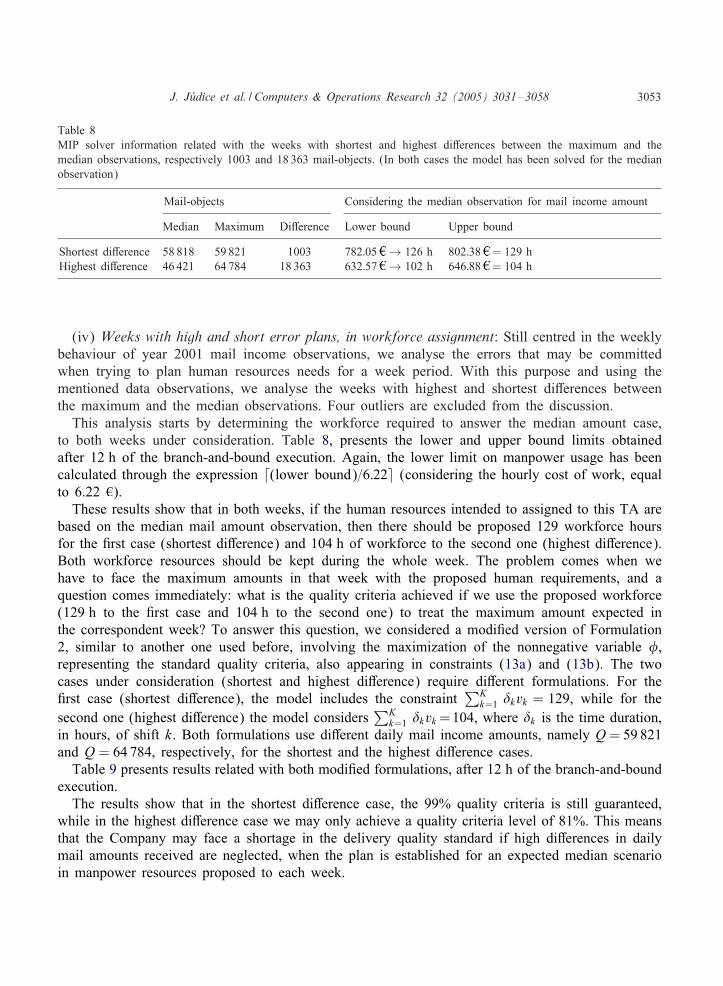
(iv) Weeks with high and short error plans, in workforce assignment: Still centred in the weeklybehaviour of year 2001 mail income observations, we analyse the errors that may be committedwhen trying to plan human resources needs for a week period. With this purpose and using thementioned data observations, we analyse the weeks with highest and shortest di4erences betweenthe maximum and the median observations. Four outliers are excluded from the discussion.

This analysis starts by determining the workforce required to answer the median amount case,to both weeks under consideration. Table 8, presents the lower and upper bound limits obtainedafter 12 h of the branch-and-bound execution. Again, the lower limit on manpower usage has beencalculated through the expression �(lower bound)=6:22� (considering the hourly cost of work, equalto 6.22 ).

These results show that in both weeks, if the human resources intended to assigned to this TA arebased on the median mail amount observation, then there should be proposed 129 workforce hoursfor the 6rst case (shortest di4erence) and 104 h of workforce to the second one (highest di4erence).Both workforce resources should be kept during the whole week. The problem comes when wehave to face the maximum amounts in that week with the proposed human requirements, and aquestion comes immediately: what is the quality criteria achieved if we use the proposed workforce(129 h to the 6rst case and 104 h to the second one) to treat the maximum amount expected inthe correspondent week? To answer this question, we considered a modi6ed version of Formulation2, similar to another one used before, involving the maximization of the nonnegative variable �,representing the standard quality criteria, also appearing in constraints (13a) and (13b). The twocases under consideration (shortest and highest di4erence) require di4erent formulations. For the6rst case (shortest di4erence), the model includes the constraint

∑Kk=1 �kvk = 129, while for the

second one (highest di4erence) the model considers∑K

k=1 �kvk=104, where �k is the time duration,in hours, of shift k. Both formulations use di4erent daily mail income amounts, namely Q= 59 821and Q = 64 784, respectively, for the shortest and the highest di4erence cases.Table 9 presents results related with both modi6ed formulations, after 12 h of the branch-and-bound

execution.The results show that in the shortest di4erence case, the 99% quality criteria is still guaranteed,

while in the highest di4erence case we may only achieve a quality criteria level of 81%. This meansthat the Company may face a shortage in the delivery quality standard if high di4erences in dailymail amounts received are neglected, when the plan is established for an expected median scenarioin manpower resources proposed to each week.


Table 9MIP solver information related with the two modi6ed formulations, proposed to maximize the quality criteria achievedwhen facing maximum mail amount quantities with a workforce established according to the median observation mailamount, to both shortest and highest di4erence scenarios

Maximum Workforce (h) Lower bound Upper bound

Shortest di4erence 59 821 m-o 129 �¿ 0:99 = 59 256 m-o �6 0:995 = 59 500 m-oHighest di4erence 64 784 m-o 104 �¿ 0:81 = 52 442 m-o �6 0:815 = 52 773 m-o

It can be showed that the 64 784 mail-objects can be treated by a workforce solution of 141 h(lower limit of 139 h), with a guaranteed quality criteria of 99%.

6. Conclusions

This paper describes an application to a batching decision process, in which the daily work-force cost of a mail processing center TA is minimized. A formulation to this problem has beenproposed. A branch-and-bound algorithm has processed the resulting optimization problem and hasbeen able to produce solutions, answering to many proposed scenarios. Those solutions have beenconsidered important for decision making support to the Company Sta4 Department. Based inthe year 2001 behaviour, workforce requirements were discussed for di4erent daily mail amountsentered in TA5, and considering di4erent levels for the quality criteria on daily total mailtreated.

Other changes on the parameters could have been considered, namely variations on the type andduration of working shifts, periods of failure in some TUs and other scenarios that have not beendiscussed in this work.

The next step of this collaboration with CTT should involve the study of the other TAs, byadapting Formulation 1 to those speci6c treatment areas. The last step should incorporate in a singlemodel all the TAs sta4 planning structure, characterizing a global environment and considering theemployees interchange among TAs. This model is more challenging, especially from the optimizationpoint of view, eventually requiring the use of decomposition techniques to obtain good solutions ina reasonable amount of time.

Acknowledgements

The authors are quite grateful to the referees for their comments and suggestions that havecontributed to improve the quality of the paper. The research of the 6rst and the second au-thors is partially supported by the projects FCT–POCTI/35059/MAT/2000 and POCTI/ISFL/152,respectively.


Appendix A

P1 matrix, where p1ri is the mail-Cow transfer rate from TUr to TUi (r; i = 1; : : : ; M) in the17:00–23:00 period

P1 =

0 0:09 0:16 0:74 0 0:007 0 0 0

0 0 0 0 0 0 0:46 0:54 0

0 0 0 0 0 0 0:36 0:64 0

0 0 0 0 0:47 0 0:25 0:28 0

0 0 0 0 0 0 0:53 0:47 0

0 0 0 0 0 0 0 1 0

0 0 0 0 0 0 0 0 1

0 0 0 0 0 0 0 0 1

0 0 0 0 0 0 0 0 0

:

P2 matrix, where P2ri is the mail-Cow transfer rate from TUr to TUi (r; i = 1; : : : ; M) in the23:00–04:00 period

P2 =

0 0 0 0 0 0 0 0 0

0 0 0 0 0 0 0 1 0

0 0 0 0 0 0 0 1 0

0 0 0 0 0:47 0 0 0:53 0

0 0 0 0 0 0 0 1 0

0 0 0 0 0 0 0 0 1

0 0 0 0 0 0 0 0 1

0 0 0 0 0 0 0 0 1

0 0 0 0 0 0 0 0 0

:

Parameters qij (i=1; : : : ; M −1, j=1; : : : ; N ) representing the number of mail-objects arrived directlyto each TU per period are given below:

Period TU1 TU2 TU3 TU4 TU5 TU6 TU7 TU8

1 → 17:00–17:15 2345 0 0 0 0 0 0 02 → 17:15–17:30 2345 0 0 0 0 0 0 03 → 17:30–17:45 0 0 0 0 0 0 0 04 → 17:45–18:00 0 0 0 0 0 0 0 05 → 18:00–18:15 0 0 0 0 0 0 0 06 → 18:15–18:30 0 0 0 0 0 0 0 07 → 18:30–18:45 0 0 0 0 0 0 0 08 → 18:45–19:00 3518 0 0 0 0 0 0 09 → 19:00–19:15 3518 0 0 0 0 0 0 0


Period TU1 TU2 TU3 TU4 TU5 TU6 TU7 TU8

10 → 19:15–19:30 3518 0 0 0 0 0 0 011 → 19:30–19:45 3518 0 0 0 0 0 0 012 → 19:45–20:00 0 0 0 0 0 0 0 013 → 20:00–20:15 3881 0 0 0 0 0 0 014 → 20:15–20:30 3881 0 0 0 0 0 0 015 → 20:30–20:45 4951 0 0 0 0 0 0 016 → 20:45–21:00 4952 0 0 0 0 0 0 017 → 21:00–21:15 1055 0 0 0 0 0 0 018 → 21:15–21:30 1055 0 0 0 0 0 0 019 → 21:30–21:45 0 0 0 0 0 0 0 0· · · · · · · · · · · · · · · · · · · · · · · · · · ·37 → 02:00–02:15 0 0 0 0 0 0 0 038 → 02:15–02:30 0 0 0 0 0 0 0 039 → 02:30–02:45 0 0 450 2078 0 8 260 040 → 02:45–03:00 0 0 450 2078 0 8 260 041 → 03:00–03:15 0 0 450 2078 0 8 260 042 → 03:15–03:30 0 0 0 0 0 0 0 043 → 03:30–03:45 0 0 0 0 0 0 0 044 → 03:45–04:00 0 0 0 0 0 0 0 0

Appendix B

Table 10 presents the number of employees determined per block and assigned to each TU:variables wih values.

Table 10Number of employees determined per block and assigned to each TU: variables wih values

One hour blocks Employees in each TU (wih)

TU1 TU2 TU3 TU4 TU5 TU6 TU7, 8 Total

17:00–18:00 0 0 0 0 0 0 0 018:00–19:00 1 0 1 1 0 0 0 319:00–20:00 2 1 1 7 2 1 2 1620:00–21:00 3 2 0 9 5 1 2 2221:00–22:00 1 1 3 6 3 0 7 2122:00–23:00 0 0 1 0 1 1 3 623:00–00:00 0 0 0 0 0 0 0 000:00–01:00 0 0 0 0 0 0 0 001:00–02:00 0 0 0 0 0 0 12 1202:00–03:00 0 0 1 6 2 0 3 1203:00–04:00 0 0 1 3 2 1 5 12


References

[1] Kuik R, Salomon M. Multi-level lot-sizing problem: evaluation of a simulated-annealing heuristic. European Journalof Operational Research 1990;45:25–37.

[2] Maes J, McClain JO, van Wassenhove LN. Multilevel capacitated lotsizing complexity and LP-based heuristics.European Journal of Operational Research 1991;53:131–48.

[3] Tempelmeier H, Helber S. A heuristic for dynamic multi-item multi-level capacitated lotsizing for general productstructures. European Journal of Operational Research 1994;75:296–311.

[4] Stadler H. Mixed integer programming model formulations for dynamic multi-item multi-level capacitated lotsizing.European Journal of Operational Research 1996;94:561–81.

[5] Tempelmeier H, Derstro4 M. A Lagrangean-based heuristic for dynamic multi-level multi-item constrained lotsizingwith setup times. Management Science 1996;42:738–57.

[6] Kimms A, Drexl A. Proportional lot sizing and scheduling: some extensions. Networks 1998;32:85–101.[7] Kuik R, Salomon M, van Wassenhove LN. Batching decisions: structure and models. European Journal of Operational

Research 1994;75:243–63.[8] Drexl A, Kimms A. Lot sizing and scheduling—survey and extensions. European Journal of Operational Research

1997;99:221–35.[9] Wolsey L. Solving multi-item lot-sizing problems with an MIP solver using classi6cation and reformulation.

Management Science 2002;48:1587–602.[10] Belvaux G, Wolsey L. Modelling practical lot-sizing problems as mixed-integer programs. Management Science

2001;47(7):993–1007.[11] Bahl HC, Ritzman LP, Gupta JND. Determining lot sizes and resource requirements: a review. Operations Research

1987;35:329–45.[12] Pochet Y, Wolsey LA. Solving multi-item lot sizing problems using strong cutting planes. Management Science

1991;37:53–67.[13] Shapiro JF. Mathematical programming models and methods for production planning and scheduling. In: Graves SC,

Rinnooy Kan AHG, Zipkin PH (editors). Handbooks in operations research and management science. Logistics ofproduction and inventory. vol. 4. Amsterdam: North-Holland; 1993 [chapter 8].

[14] Belvaux G, Wolsey L. Lot-sizing problems: modelling issues and a specialized branch-and-cut system BC-PROD.Core Discussion Paper 9849, 1998.

[15] Pochet Y. Mathematical programming models for deterministic production planning problems. In: J]unger M,Naddef D, editors. Computational combinatorial optimization. Lecture notes in computer science, vol. 2241. Berlin,Heidelberg: Springer; 2001. p. 57–111.

[16] Bechtold SE, Jacobs LW. The equivalence of general set-covering and implicit integer programming formulationsfor shift scheduling. Naval Research Logistics 1996;43:233–49.

[17] Aykin T. A comparative evaluation of modelling approaches to the labor shift scheduling problem. European Journalof Operational Research 2000;125:381–97.

[18] Caprara A, Monaci M, Toth P. Models and algorithms for a sta4 scheduling problem. Mathematical ProgrammingSeries B 2003;98:445–76.

[19] Mehrotra A, Murphy KE, Trick MA. Optimal shift scheduling: a branch-and-price approach. Naval Research Logistics2000;47:185–200.

[20] Tien JM, Kamiyama A. On manpower scheduling algorithms. SIAM Review 1982;24(3):275–87.[21] Ernst AT, Jiang H, Krishnamoorthy M, Sier D. Sta4 scheduling and rostering: a review of applications, methods

and models. European Journal of Operational Research 2004;153:3–27.[22] Bodin L, Golden B, Assad A, Ball M. Routing and scheduling of vehicles and crews—the state of the art. Computers

and Operations Research 1983;10(2):63–211.[23] Caprara A, Fischetti M, Toth P, Vigo D, Guida PL. Algorithms for railway crew management. Mathematical

Programming 1997;79:125–41.[24] Vance PH, Barnhart C, Johnson EL, Nemhauser GL. Airline crew scheduling: a new formulation and decomposition

algorithm. Operations Research 1997;45(2):188–200.[25] Gamache M, Soumis F, Marquis G, Desrosiers J. A column generation approach for large-scale aircrew rostering

problems. Operations Research 1999;47(2):247–63.


[26] Dawid H, K]onig J, Strauss C. An enhanced rostering model for airline crews. Computers and Operations Research2001;28:671–88.

[27] Fischetti M, Lodi A, Martello S, Toth P. A polyhedral approach to simpli6ed crew scheduling and vehicle schedulingproblems. Management Science 2001;47(6):833–50.

[28] Dijkstra MC, Kroon LG, Salomon M, van Nunen JAEE, van Wassenhove LN. Planning the size and organizationof KLM’s aircraft maintenance personnel. Interfaces 1994;24(6):47–58.

[29] Brusco MJ, Jacobs LW, Bongiorno RJ, Lyons DV, Tang B. Improving personnel scheduling at airline stations.Operations Research 1995;43(5):741–51.

[30] Mason AJ, Ryan D, Panton DM. Integrated simulation, heuristic and optimisation approaches to sta4 scheduling.Operations Research 1998;46(2):161–75.

[31] Segal M. The operator-scheduling problem: a network-Cow approach. Operations Research 1974;22:808–23.[32] Lin CKY, Lai KF, Hung SL. Development of a workforce management system for a customer hotline service.

Computers and Operations Research 2000;27:987–1004.[33] Balakrishnan N, Wong RT. A network model for the rotating workforce scheduling problem. Networks 1990;20:

25–42.[34] Jaumard B, Semet F, Vovor T. A generalized linear programming model for nurse scheduling. European Journal of

Operational Research 1998;107:1–18.[35] Bellanti F, Carello G, Della Croce F, Tadei R. A greedy-based neighborhood search approach to a nurse rostering

problem. European Journal of Operational Research 2004;153:28–40.[36] Malhotra MK, Ritzman LP, Benton WC, Keong Leong G. A model for scheduling postal distribution employees.

European Journal of Operational Research 1992;58:374–85.[37] Jarrah AIZ, Bard JF, deSilva AH. Solving large-scale tour scheduling problems. Management Science

1994;40(9):1124–44.[38] Bard JF, Binici C, deSilva AH. Sta4 scheduling at the United States Postal Service. Computers and Operations

Research 2003;30:745–71.[39] Ilog Inc. ILOG CPLEX User’s Manual, Version 7.0. Ilog Inc., 2000.[40] SPSS 11.0 Applications guide. Chicago IL: SPSS Inc.; 2002.

workforce planning in a lotsizing mail processing … planning in a lotsizing mail processing...

Documents