WOLF DEN SITE SELECTION AND CHARACTERISTICS

IN THE NORTHERN ROCKY MOUNTAINS:

A MULTI-SCALE ANALYSIS

Jon R. Trapp

May 2004

ii

WOLF DEN SITE SELECTION AND CHARACTERISTICSIN THE NORTHERN ROCKY MOUNTAINS: A MULTI-SCALE ANALYSIS

A ThesisBy

Jon R. Trapp

Submitted in partial fulfillment of therequirements for the degree of

Master of Arts from Prescott College inEnvironmental Studies – Conservation Biology

Approved as to style and content by:

___________________________ ____________________________ David R. Parsons Paul Beier (Committee Chair) (Member)

___________________________ ____________________________Paul C. Paquet Curt Mack

(Special Member) (Special Member)

___________________________ Paul G. Sneed (Head of Department)

May 2004

iii

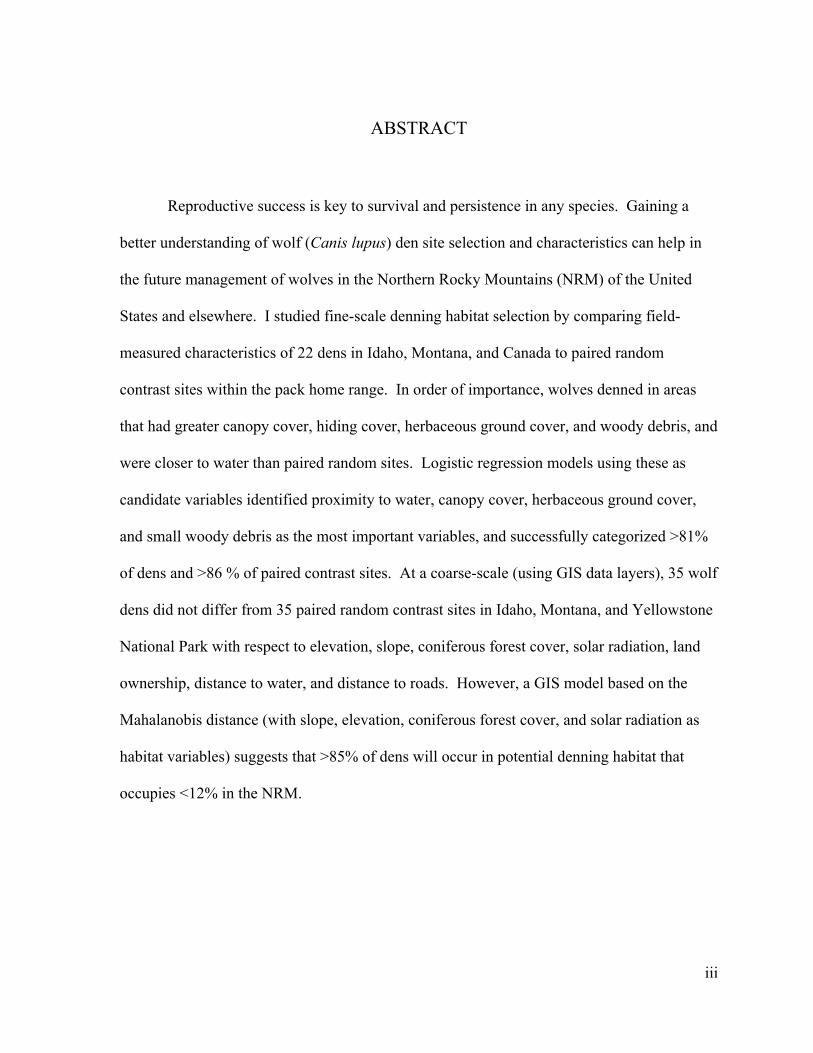
ABSTRACT

Reproductive success is key to survival and persistence in any species. Gaining a

better understanding of wolf (Canis lupus) den site selection and characteristics can help in

the future management of wolves in the Northern Rocky Mountains (NRM) of the United

States and elsewhere. I studied fine-scale denning habitat selection by comparing field-

measured characteristics of 22 dens in Idaho, Montana, and Canada to paired random

contrast sites within the pack home range. In order of importance, wolves denned in areas

that had greater canopy cover, hiding cover, herbaceous ground cover, and woody debris, and

were closer to water than paired random sites. Logistic regression models using these as

candidate variables identified proximity to water, canopy cover, herbaceous ground cover,

and small woody debris as the most important variables, and successfully categorized >81%

of dens and >86 % of paired contrast sites. At a coarse-scale (using GIS data layers), 35 wolf

dens did not differ from 35 paired random contrast sites in Idaho, Montana, and Yellowstone

National Park with respect to elevation, slope, coniferous forest cover, solar radiation, land

ownership, distance to water, and distance to roads. However, a GIS model based on the

Mahalanobis distance (with slope, elevation, coniferous forest cover, and solar radiation as

habitat variables) suggests that >85% of dens will occur in potential denning habitat that

occupies <12% in the NRM.

iv

ACKNOWLEDGEMENTS

This research project would not have been possible without the support and trust

given by Curt Mack with the Nez Perce Wolf Project and Carter Niemeyer with the U.S. Fish

and Wildlife Service (USFWS). I also thank Ed Bangs with the USFWS for supporting this

research throughout the Northern Rocky Mountains. Funding was provided by the Nez Perce

Tribe, the USFWS, the Wolf Education and Research Center, the Shikari Tracking Guild,

and Fischer Enterprises.

I am grateful to my principal advisor, David Parsons, for his constant encouragement

and helpful suggestions. David has made my educational experience a challenging and

rewarding journey. I also appreciate the support and guidance of my other committee

members; Paul Beier (Northern Arizona University), Curt Mack, Paul Paquet (University of

Calgary), and Paul Sneed (Prescott College). Edward Garton (University of Idaho) provided

advice on different techniques for statistical analysis. Leona Svancara and Gina Wilson at

the Landscape Dynamics Lab (University of Idaho) graciously provided their time and

computers in running GIS computations. Thanks to Jeff Cronce with the Nez Perce Tribe for

helping with GIS issues. Jeff Jenness (Jenness Enterprises) was always available to answer

GIS questions and provide solutions.

I also thank Joe Fontaine, Tom Meier, and Steve Fritts, of the USFWS. Doug Smith

and Deb Guernsey of the Yellowstone Wolf Project provided insight and data that helped to

shape this project. Thanks to John Waller with Glacier National Park for gathering a search

party and allowing access to dens. Finding dens in Idaho was made easier by the hard work

of the Nez Perce Wolf Project biologists Jim Holyan, Isaac Babcock, Kent Laudon, Adam

v

Gall, Jason Husseman, and Anthony Novak. Dan Davis (Clearwater National Forest) helped

to locate a den in Idaho. I also appreciate the logistical support provided by Consuelo Blake

in the Nez Perce Wolf Project office.

I could not have completed this project without the tireless support of my field

assistants Casey King, Rob LaBuda, and Barbara Trapp. Their dedication and positive

attitude will be long appreciated. Barbara Trapp also provided expertise in designing a new

database to store the den data. I also appreciate the help of Casey Brown, Emily Babcock,

Jay Mallonee, Jon Young (Shikari Tracking Guild), and Henning Stabins (Plum Creek

Timber Company).

Equipment was provided by the Nez Perce Tribe, Payette National Forest, and

Prescott College. Thank you to Caleb Zurstadt (Payette National Forest) for support in the

office. We wouldn’t have covered the nearly 20,000 miles without the Jeep provided by the

Nez Perce Tribe and Gerry Herker of GSA. The ArcView training provided by the

Geographic Data Service Center (CO) helped substantially with my GIS work. Thanks to

Tom Davidson and Jeff Truscott, Banff National Park, for taking us into 2 wolf dens and

providing GIS support. Thanks to the Sun Ranch in Montana and the Coiner Ranch in Idaho

for allowing access to wolf dens. Soil samples were analyzed by the University of Idaho Soil

Evaluation Team.

And thank you to the small school with a big heart. Prescott College faculty members

and staff have provided continual support and guidance through this process. I especially

want to thank Lyn Chenier, Linda Butterworth, and Norma Mazur for their outstanding work

in the library.

vi

DEDICATION

This is dedicated to my wife Barbara, who is always there to bring me up when I am

down, and to celebrate the victories with me. Her support, patience, and understanding have

been an inspiration. I also dedicate this to my parents, Ted and Jackie, who have always

supported the tough decisions in my life – especially the one to leave the Air Force to

become a wildlife biologist.

vii

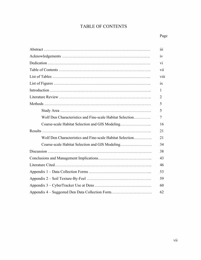
TABLE OF CONTENTS

Page

Abstract ……………………………………………………………………… iii

Acknowledgements …………………………………………………………. iv

Dedication …………………………………………………………………… vi

Table of Contents ……………………………………………………………. vii

List of Tables ………………………………………………………………... viii

List of Figures ……………………………………………………………….. ix

Introduction ………………………………………………………………….. 1

Literature Review ……………………………………………………………. 2

Methods ……………………………………………………………………… 5

Study Area …………………………………………………………… 5

Wolf Den Characteristics and Fine-scale Habitat Selection…………. 7

Coarse-scale Habitat Selection and GIS Modeling…………………... 16

Results ……………………………………………………………………….. 21

Wolf Den Characteristics and Fine-scale Habitat Selection………….. 21

Coarse-scale Habitat Selection and GIS Modeling…………………… 34

Discussion ……………………………………………………………………. 38

Conclusions and Management Implications………………………………….. 43

Literature Cited……………………………………………………………….. 46

Appendix 1 – Data Collection Forms ………………………………………... 53

Appendix 2 – Soil Texture-By-Feel …………………………………………. 59

Appendix 3 – CyberTracker Use at Dens ……………………………………. 60

Appendix 4 – Suggested Den Data Collection Form…………………………. 62

viii

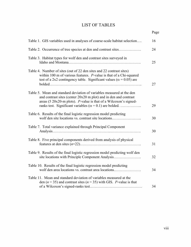
LIST OF TABLES

Page

Table 1. GIS variables used in analyses of coarse-scale habitat selection…. 16

Table 2. Occurrence of tree species at den and contrast sites……………… 24

Table 3. Habitat types for wolf den and contrast sites surveyed inIdaho and Montana…………………………………………………. 25

Table 4. Number of sites (out of 22 den sites and 22 contrast sites)within 100 m of various features. P-value is that of a Chi-squaredtest of a 2x2 contingency table. Significant values (α = 0.05) arebolded……………………………………………………………….. 27

Table 5. Mean and standard deviation of variables measured at the denand contrast sites (center 20x20 m plot) and in den and contrastareas (5 20x20-m plots). P-value is that of a Wilcoxon’s signed-ranks test. Significant variables (α = 0.1) are bolded. …………….. 29

Table 6. Results of the final logistic regression model predictingwolf den site locations vs. contrast site locations.………………….. 30

Table 7. Total variance explained through Principal ComponentAnalysis……………………………………….……………………. 30

Table 8. Five principal components derived from analysis of physicalfeatures at den sites (n=22)…………………………………………. 31

Table 9. Results of the final logistic regression model predicting wolf densite locations with Principle Component Analysis…………………. 32

Table 10. Results of the final logistic regression model predictingwolf den area locations vs. contrast area locations.………………… 34

Table 11. Mean and standard deviation of variables measured at theden (n = 35) and contrast sites (n = 35) with GIS. P-value is thatof a Wilcoxon’s signed-ranks test…………………………………… 34

ix

LIST OF FIGURESPage

Figure 1. Northern Rocky Mountain gray wolf experimental population areas: northwest Montana (non-shaded area), Greater Yellowstone(dotted area), and central Idaho (hatched area). The areas in darkgray represent the core restoration areas……………………………. 5

Figure 2. Den sites (n = 37) for both fine and course-scale analysisincluded in this study……………………………………………….. 6

Figure 3. Plot layout for fine-scale denning habitat analysis. For eachden area or contrast area, there was a center point (the “den site”),and 4 satellite points at 50 m in the 4 cardinal directions.Three 20-m transects were associated with each of the 5 points.The term “den area” refers to the combined measurements acrossthe 5 points………………………………………………………….. 9

Figure 4. Area included for Mahalanobis analysis with dens usedto generate mean vector and covariance data………………………. 19

Figure 5. Hillside excavation wolf den…………………………………….. 22

Figure 6. Wolf trail leading to den site…………………………………….. 23

Figure 7. Soil texture triangle.……………………...……………………… 26

Figure 8. General aspects of den and contrast sites; octagons indicatenumber of dens (e.g., 4 dens with a NW aspect). Dens aredepicted by solid gray and contrast sites by the dashed line………… 28

Figure 9. Plot of principal component 3 (corresponding to increasingherbaceous cover and small logs, greater probability of waterwithin 100 m, and fewer rocks and shrubs) and principalcomponent 1 (corresponding to more hiding cover, canopy cover,trees, shrubs, water; lower elevation, and exposed soil)……..……… 33

Figure 10. Example of den site, telemetry locations, fixed kernel homeranges (95 and 50%), and the MCP home range. The larger lightpolygons are part of the 95% kernel home range, and the smalldark polygon is the core 50% kernel. The telemetry locations arethe dots and the star is the den. The hollow polygon with thestraight lines is the MCP home range………………………………. 35

x

Page

Figure 11. Example of Mahalanobis output for central Idaho withden sites……………………………..………………………………. 36

Figure 12. Percent of dens (dashed line) or cells (solid line) withMahalanobis-P greater than or equal to threshold value. Highervalues along the x-axis indicate greater similarity to the meanvector of habitat measurements at 35 wolf dens.…………………… 37

Figure A-1. Soil texture-by-feel flow chart.……………………………… 59

Figure A-2. CyberTracker data collected at den site…………………….. 60

1

INTRODUCTION

Wolves are one of the most studied mammals in the world. Multiple studies have

focused on wolf reproduction and denning (e.g., Mech 1970; Ballard and Dau 1983; Fuller

1989; Ciucii and Mech 1992; Matteson 1992; Unger 2003), but den site selection in forested

ecosystems is not completely understood (Norris et al. 2002). Because most pup mortality

occurs within the first 6 months, site selection and activity around the den affect reproductive

success of the pack (Harrington and Mech 1982). This study is the first to examine wolf den

site selection in the NRM since the reintroductions in central Idaho and Yellowstone

National Park in 1995-96, and is based on a larger number of dens than any previous study of

den site selection.

The purpose of this research is to better understand wolf den site selection and

characteristics to support effective, long-term conservation and management of wolves. The

objectives are threefold: 1) to determine wolf den site characteristics; 2) to investigate

factors influencing den site selection at fine and course scales; and 3) to develop a predictive

denning habitat model utilizing a Geographic Information System (GIS).

2

LITERATURE REVIEW

Wolves are social animals that form family groups called packs, ranging in size from

2 to more than 30 individuals. A wolf pack usually consists of the dominant pair (usually the

parents) and their subordinate young (Mech 1970). Wolves generally establish territories

that can cover as much as 2,500 km2 (Mech et al. 1998), but average 579 km2 in Idaho, 554

km2 in the Greater Yellowstone Area, and 298 km2 in northwest Montana (USFWS et al.

2001). Territories are defended passively and actively from other packs.

The breeding season is from January to April, depending upon latitude (Mech 1970).

Usually, only the dominant pair breeds (Paquet and Carbyn 2003). Gestation lasts 62-63

days with parturition generally in some sort of sheltered area (Mech 1970). The average

whelping date is 11 April for pregnant wolves in Yellowstone National Park (Thurston

2002). Litter size can range from one to 11, and averages 6 (Paquet and Carbyn 2003). Pups

generally remain at the den site for 8 to 10 weeks before moving to their first rendezvous site

(Murie 1944; Peterson 1977). Other pack members may assist in the pup rearing by

providing defense (Mech 2000), feeding the nursing mother (Mech et al. 1999), or

regurgitating food when the pups are older.

Denning habitat for tundra wolves may be a limiting factor (McLoughlin et al. 2004).

In the tundra, esker habitat, which comprised only 1-2% of the landscape, was the preferred

denning habitat. Wolves in Algonquin Provincial Park, Canada, prefer to den in pine forests

(Norris et al. 2002). However, these pine forests are frequently and extensively logged,

removing potential denning habitat. Repeated use of dens by wolves (Ballard and Dau 1983;

3

Mech and Packard 1990) suggests they are valuable habitat elements, and perhaps at times a

limiting factor.

Techniques and results of the following studies guided the design and evaluation of

this study. Studies of wolf dens have examined site location within home ranges (Ciucci and

Mech 1992; Unger 1999), location in relation to prey availability (Banfield 1954; Carbyn

1975; Boertje and Stephenson 1992), effects of human disturbance (Mech 1989; Thiel et

al.1998), and micro-habitat variables (Matteson 1992; Norris et al. 2002). GIS studies

evaluated habitat variables involved in territory selection (Haight et al. 1998; Mladenoff et al.

1999; Houts 2001; Oakleaf 2002; Carrol et al. 2003), effects of road density on habitat

suitability (Wydeven et al. 2001 ), and the Mahalanobis distance (Clark et al. 1993; Corsi et

al. 1999; Podruzny et al. 2002; Farber and Kadmon 2003). A transect method for evaluating

physical and vegetative characteristics at bobcat (lynx rufus) rest sites used by Kolowski and

Woolf (2002) was modified for this study.

This study adds to Matteson’s (1992) evaluation of dens (n = 15) in northern Montana

and southern Canada. She found that wolves selected sites at lower elevations (e.g., valley

bottoms and lower slopes) with less percent slope. Dens were also closer to hiking and horse

packing trails than contrast locations. Variables found by Matteson (1992) to be insignificant

included canopy cover, hiding cover, ecotype, structural class, solar radiation, and distance to

water. A study of 13 dens by Unger (1999) in northwest Wisconsin and east-central

Minnesota found steep slope, sandy soil, lower road density, and close proximity to water to

be significant variables. Insignificant variables included canopy cover and hiding cover.

GIS analyses of wolf dens were completed by Unger (1999) and Norris et al. (2002).

Unger’s (1999) GIS analysis focused on the den site location within the Minimum Convex

4

Polygon (MCP) home range. He found that dens tended to be in the inner core of the MCP.

This contradicts a study by Ciucci and Mech (1992), which found dens located randomly

throughout home ranges. In Algonquin Provincial Park Norris et al. (2002) found dens (n =

16) to be in areas with a high proportion of pine forests. They also found that dens were at

lower elevations and near water. Studies by Clark et al. (1993) and Podruzny et al. (2002)

applied GIS and the Mahalanobis distance statistic to model bear habitat and den sites.

5

METHODS

Study Area

This study was focused in the 3 United States Northern Rocky Mountains (NRM)

wolf recovery areas: northwestern Montana, central Idaho, and the Greater Yellowstone area

(Fig. 1). At the end of 2003, there were an estimated 368 wolves in the central Idaho

recovery area, 301 in the Greater Yellowstone area, and 92 in northwestern Montana

(USFWS et al. 2004). Den sites were visited in Idaho, Montana, and southern Canada to

examine wolf den characteristics and fine-scale habitat selection. Additional den sites from

Yellowstone National Park were included in the course-scale habitat selection and GIS

modeling analyses (Fig. 2).

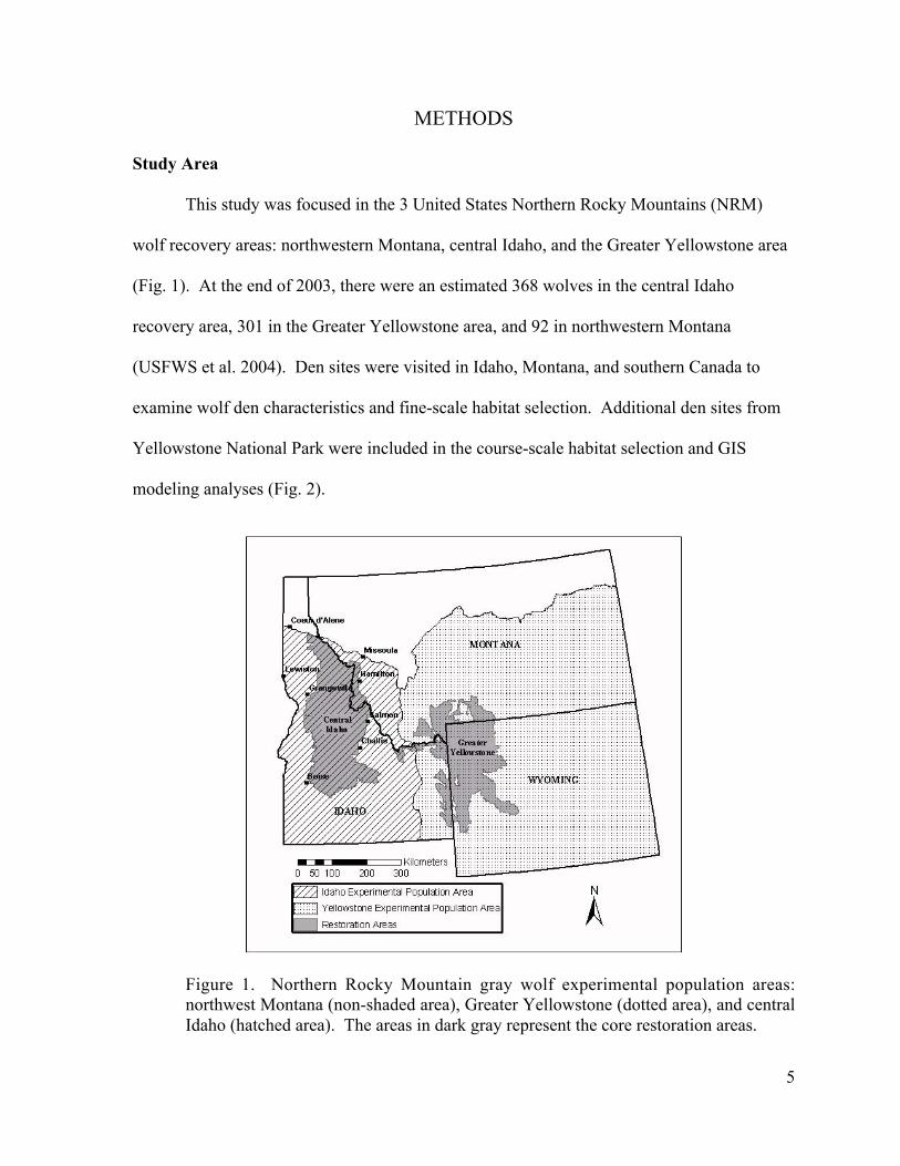
Figure 1. Northern Rocky Mountain gray wolf experimental population areas:northwest Montana (non-shaded area), Greater Yellowstone (dotted area), and centralIdaho (hatched area). The areas in dark gray represent the core restoration areas.

6

The NRM extend from the Salt River and Wind River ranges in Wyoming to the

northern borders of western Montana and Idaho. This mountain range is bounded by the

Great Plains to the east and the Columbia Plateau and Great Basin to the west. The major

factor in the formation of these mountains has been volcanic activity (Kershaw et al. 1998).

Receding glaciers have smoothed plains, cut broad valleys, and formed dramatic peaks in

other areas. Some of the highest peaks include Gannett Peak (4,183 m) in Wyoming, Granite

Peak (3,878 m) in Montana, and Borah Peak (3,837 m) in Idaho.

^̀

^̀̀̂^̀^̀^̀

^̀^̀^̀̀̂

^̀

^̀

^̀^̀^̀^̀^̀

^̂̀`

^̀^̀^̀ ^̀̀̂^̀

^̀^̀ ^̂̀`̀̀̂̂^̀^̀̂̀̀̂^̀

153812.732

153812.732

397815.314

397815.314

641817.896

641817.896

885820.478

885820.478

1129823.061

1129823.061

1373825.643

1373825.643

4532337.409

45 32337.409

4780719.873

47 80719.873

5029102.337

50 29102.337

5277484.802

52 77484.802

5525867.266

55 25867.266

5774249.730

57 74249.730

Montana

WyomingIdaho

Canada

±

0 380 760190 Kilometers

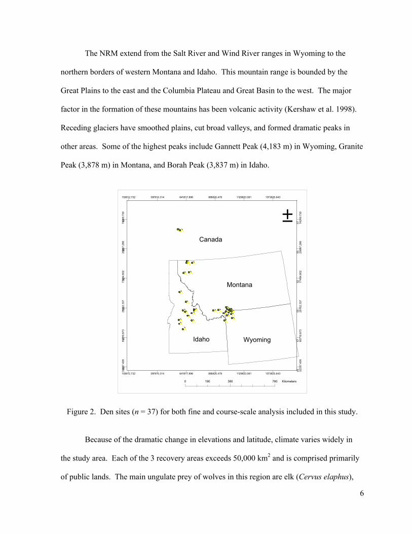
Figure 2. Den sites (n = 37) for both fine and course-scale analysis included in this study.

Because of the dramatic change in elevations and latitude, climate varies widely in

the study area. Each of the 3 recovery areas exceeds 50,000 km2 and is comprised primarily

of public lands. The main ungulate prey of wolves in this region are elk (Cervus elaphus),

7

white-tailed deer (Odocoileus virginianus), mule deer (O. hemionus), and moose (Alces

alces).

Wolf Den Characteristics and Fine-scale Habitat Selection

Thirty-two dens were visited between June and October 2003. Known and suspected

den site locations were provided by the Nez Perce Tribe in Idaho, USFWS in Montana, and

Banff National Park in Alberta. Some dens were found by evaluating aerial telemetry

locations of collared wolves during the denning season (April-June). I gave priority to dens

used since 2000. To minimize impact to wolves, data collection at the den sites did not start

until June, when packs start moving away from their dens (Haber 1968). Aerial and ground

telemetry of collared wolves confirmed when they had moved away. In case uncollared pups

were in dens, we moved into den areas quietly and slowly. Data collection began after

confirming that the pack had departed the den. The field crew hiked to the derived

coordinates utilizing a Global Positioning System (GPS). If the den was not found

immediately, the crew split up and searched likely locations. When these search methods

failed to locate the den, a grid search pattern was conducted.

Because wolves often use the same den in subsequent years (Ballard and Dau 1983;

Mech and Packard 1990), we took precautions not to modify the den site. If the entrance

dimensions did not allow entry to the main chamber to take measurements, we did not

modify the entrance, and estimated dimensions visually. Because wolves are known to visit

the dens throughout the year (Peterson 1977), precautions were taken to minimize our scent

in the area (e.g., when necessary, urinating >150 m from the den).

8

Not all dens were suitable for analysis. Some dens were excluded for the following

reasons: 1) last used prior to the year 2000; 2) uncertainty of site being the natal den; and 3)

habitat modification since use (e.g., logging). We collected complete data at 25 dens (15 in

Idaho, 8 in Montana, and 2 in Banff National Park, Canada).

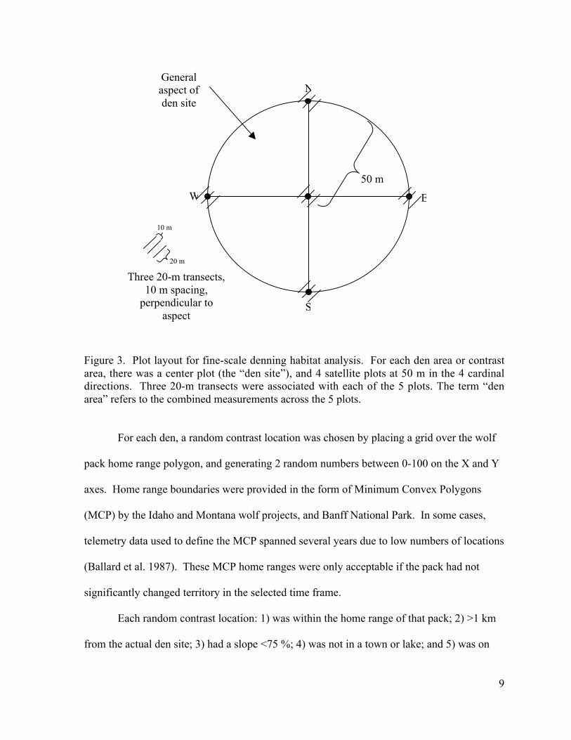
Field data were collected at 5 locations per site: the den hole (center plot) and at 50

meters in each cardinal direction (50-m plots) (Fig. 3). Data collected at the center plot were

used to characterize the “site,” whereas the 50-m plots and the center plot were used to

describe the “area.” Three 20-m transects were placed perpendicular to the aspect of the hill

and spaced 10 m apart at each plot. Plots covered a 20 x 20 m area.

9

Figure 3. Plot layout for fine-scale denning habitat analysis. For each den area or contrastarea, there was a center plot (the “den site”), and 4 satellite plots at 50 m in the 4 cardinaldirections. Three 20-m transects were associated with each of the 5 plots. The term “denarea” refers to the combined measurements across the 5 plots.

For each den, a random contrast location was chosen by placing a grid over the wolf

pack home range polygon, and generating 2 random numbers between 0-100 on the X and Y

axes. Home range boundaries were provided in the form of Minimum Convex Polygons

(MCP) by the Idaho and Montana wolf projects, and Banff National Park. In some cases,

telemetry data used to define the MCP spanned several years due to low numbers of locations

(Ballard et al. 1987). These MCP home ranges were only acceptable if the pack had not

significantly changed territory in the selected time frame.

Each random contrast location: 1) was within the home range of that pack; 2) >1 km

from the actual den site; 3) had a slope <75 %; 4) was not in a town or lake; and 5) was on

N

EW

S

Three 20-m transects,10 m spacing,

perpendicular toaspect

Generalaspect ofden site

10 m

20 m

50 m

10

public land or private property with landowner consent for our research. In 4 cases where no

home range data were available, contrast locations were established 1 km away in a random

compass direction.

The following variables were measured at the center plot of each den area. Except as

noted below, these variables were also measured at the center plot of each contrast location.

Acronyms for the variables used in the logistic regression analysis are given in upper case

within parentheses after each variable name. Field forms are presented in Appendix 1.

Location: Den and contrast site coordinates were determined using a GPS unit (Garmin TM

eTrex Summit) and recorded in Universal Transverse Mercator (UTM) format referenced to

North American Datum, 1927. Coordinates were not locked into the GPS until the estimated

accuracy was <10 m.

Elevation (ELEVATION) was recorded in meters determined from the GPS unit.

Den Type Description and Measurements: We categorized den type as hillside excavation,

tree root crown, boulder pile, or as a combination (e.g., hillside excavation in root crown).

Height and width of entrance and interior chamber, as well as depth, were recorded when

possible. We also sketched the den site (Appendix 1). These data were only collected at the

den site.

11

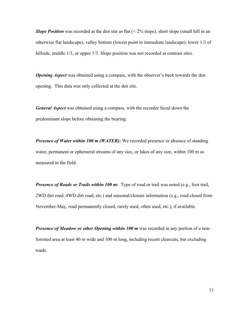
Slope Position was recorded at the den site as flat (< 2% slope), short slope (small hill in an

otherwise flat landscape), valley bottom (lowest point in immediate landscape), lower 1/3 of

hillside, middle 1/3, or upper 1/3. Slope position was not recorded at contrast sites.

Opening Aspect was obtained using a compass, with the observer’s back towards the den

opening. This data was only collected at the den site.

General Aspect was obtained using a compass, with the recorder faced down the

predominant slope before obtaining the bearing.

Presence of Water within 100 m (WATER): We recorded presence or absence of standing

water, permanent or ephemeral streams of any size, or lakes of any size, within 100 m as

measured in the field.

Presence of Roads or Trails within 100 m: Type of road or trail was noted (e.g., foot trail,

2WD dirt road, 4WD dirt road, etc.) and seasonal/closure information (e.g., road closed from

November-May, road permanently closed, rarely used, often used, etc.), if available.

Presence of Meadow or other Opening within 100 m was recorded in any portion of a non-

forested area at least 40 m wide and 100 m long, including recent clearcuts, but excluding

roads.

12

Presence of Human Habitation/Disturbance within 100 m. We included mining, active

logging operations, and human structures within 100 m of the site.

Presence of Rock Outcrop within 100 m of the den or contrast site.

Structural Class: We recorded the dominant vegetation class within the 20 x 20 m plot

delineated by the transect grid as: non-vegetated, herbaceous, shrub, sapling, pole/sapling,

young/mature, old-growth.

Soil Composition: Samples were taken from inside the den-hole and collected in a plastic

bag labeled with the pack name and year used. Soil type (e.g., sand, loam, silt, clay, etc.)

was analyzed using the “Texture-by-feel” method (Thien 1979). Soil samples were not taken

at contrast sites.

Habitat Type was determined using U.S. Forest Service documents: Forest Habitat Types of

Central Idaho (Steele et al. 1981), Forest Habitat Types of Northern Idaho (Cooper et al.

1991), and Forest Habitat Types of Montana (Pfister et al. 1977).

13

The following variables were measured at each of the 5 plots in both den areas and contrast

areas:

Slope (SLOPE) percentage was determined using a clinometer. We averaged the slope along

the fall line 10 m upslope and downslope from each point.

Hiding Cover (COVER) was recorded as the average percent obscured of a 2 m high cover

pole observed from 10 m away in each cardinal direction (Griffith and Youtie 1988). The

observer viewed the pole from a crouched position in the center of the plot. The cover pole

was divided into 20 1-decimeter (dm) sections. Data were recorded as a percentage of 1-dm

sections obscured by vegetative or structural (e.g., boulders, hillside) cover.

Canopy Density (CANOPY) was estimated using a spherical densiometer (Lemon 1957),

because it is more likely to reflect an animal’s perception of cover than point-intercept

measures of cover (Nuttle 1997). We averaged the readings taken in 4 cardinal directions at

each of 5 plots.

Major Tree and Shrub Species: We recorded each tree species with at least 10 individuals

within the 20 x 20 m plot, and each shrub that covered at least 10% of the ground within the

plot.

Ground Cover: At each 1-m interval along the 3 transects (Figure 3), we assigned one

ground cover category, and converted counts to percentage by dividing by the 63 (number of

14

possible hits). The categories were: Herbaceous (HERB, including shrubs <20 cm tall);

Leaf/Needle Litter (LITTER, including woody material <5 cm in diameter); Shrub

(SHRUB, plants 20 to 200 cm tall); Small Wood (SMALL WOOD, 5-15 cm diameter at

midpoint); Log (LOG, >15 cm diameter); Rock (ROCK, >1” diameter); Soil (SOIL), or Tree

(TREE, touching tape, including exposed root system, >200 cm tall).

Index of Tree Diameter: We measured diameter of each tree >2” DBH touching the transect

tape, and tallied smaller trees (using 1” as a diameter in calculating means). Because the

transect tape is deflected by larger trees and the crowns of saplings, this method may

undersample medium-sized trees. Therefore, it was used only to compare den and contrast

sites and areas. We did not record diameters separately by species.

Additional Observations: This category was used to record any other potentially useful

information. Data recorded included observations on other predator activity, bones, wolf

scats and daybeds, trails, etc.

To describe wolf den sites I created frequency distributions of structural class, tree

species, shrub species, and habitat type. Soil composition was analyzed and described at the

den sites only. I compared number of den and contrast sites within 100 m of roads/trails,

meadow/opening, human disturbance, and rock outcrop, and tested for significant differences

using Chi-square tests. I calculated mean and standard deviation (SD) for elevation, slope,

hiding cover, canopy density, tree diameter index, and 8 ground cover classes at both den and

15

contrast sites. I created a radar graph to depict frequency distributions of general aspects at

den and contrast sites.

I excluded 3 of the 15 dens in Idaho from the fine-scale univariate analysis, because

contrast site data were not obtained. The Wilcoxon’s signed-ranks test (Zar 1999) was used

to compare den and contrast areas and sites with respect to 13 variables: ELEVATION,

SLOPE, COVER, CANOPY, WATER, and 8 ground cover categories (HERB, LITTER,

SHRUB, SMALL WOOD, LOG, ROCK, SOIL, and TREE).

I created forward entry logistic regression models at the site (1-plot) and area (5-plot)

scales. Variables significantly different (Wilcoxon’s signed-ranks test, α = 0.10) between den

and contrast sites or areas were evaluated for multicollinearity. If Pearson Correlation (Zar

1999) coefficients indicated correlation (|r| >0.50), variables with lower P-values were

removed from the list of candidate variables. The criteria for variables to enter and remain in

the logistic regression model was P < 0.20 (Hosmer and Lemeshow 2000), using P-values

associated with each variable’s R statistic.

Because univariate methods (e.g., Wilcoxon’s signed-ranks test) can fail to address

confounding of highly correlated variables, I also used Principal Component Analysis (PCA)

(Ramsey and Schafer 1997) to characterize den sites and areas. I used the same 13 variables

to derive the principal components. Principle components with initial eigenvalues >1 were

used as candidate variables in a forward-entry logistic regression model. The criteria for

components was P < 0.05 to enter, and P > 0.1 for removal (Hosmer and Lemeshow 2000),

using P-values associated with each component’s R statistic.

All statistical analyses were completed using SPSS (SPSS 8.0 1997).

16

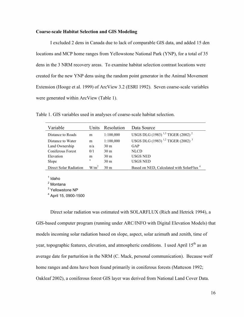
Coarse-scale Habitat Selection and GIS Modeling

I excluded 2 dens in Canada due to lack of comparable GIS data, and added 15 den

locations and MCP home ranges from Yellowstone National Park (YNP), for a total of 35

dens in the 3 NRM recovery areas. To examine habitat selection contrast locations were

created for the new YNP dens using the random point generator in the Animal Movement

Extension (Hooge et al. 1999) of ArcView 3.2 (ESRI 1992). Seven coarse-scale variables

were generated within ArcView (Table 1).

Table 1. GIS variables used in analyses of coarse-scale habitat selection.

Variable Units Resolution Data SourceDistance to Roads m 1:100,000 USGS DLG (1983) 1,3 TIGER (2002) 2

Distance to Water m 1:100,000 USGS DLG (1983) 1,2 TIGER (2002) 3

Land Ownership n/a 30 m GAPConiferous Forest 0/1 30 m NLCDElevation m 30 m USGS NEDSlope ° 30 m USGS NED

Direct Solar Radiation W/m2 30 m Based on NED, Calculated with SolarFlux 4

1 Idaho2 Montana3 Yellowstone NP4 April 15, 0900-1500

Direct solar radiation was estimated with SOLARFLUX (Rich and Hetrick 1994), a

GIS-based computer program (running under ARC/INFO with Digital Elevation Models) that

models incoming solar radiation based on slope, aspect, solar azimuth and zenith, time of

year, topographic features, elevation, and atmospheric conditions. I used April 15th as an

average date for parturition in the NRM (C. Mack, personal communication). Because wolf

home ranges and dens have been found primarily in coniferous forests (Matteson 1992;

Oakleaf 2002), a coniferous forest GIS layer was derived from National Land Cover Data.

17

Coniferous forest layer was developed as a percentage of forested cells within 100 m of the

den or contrast site. Elevation and slope were derived from National Elevation Data (NED).

I determined land ownership with Gap Analysis Program (GAP) land ownership layers

(USGS 2002). Road and water data were derived from USGS Digital Line Graphs (DLG)

and Topologically Integrated Geographic Encoding and Referencing system (TIGER) (USSB

2002). Distances from dens to water and roads were calculated with distance functions in

ArcView. In my analyses I did not distinguish among 4 TIGER road classes (primary

highways with limited access, primary roads without limited access, secondary and

connecting roads, and local, neighborhood and rural roads).

Habitat Selection. Variables significantly different (Wilcoxon’s signed-ranks test, α

= 0.10) between den sites and contrast sites were evaluated for multicollinearity as measured

by Pearson Correlation coefficients. If there was a correlation (|r| > 0.50), then variables

with lower T-statistics were removed. The remaining variables were then used as candidate

variables in a forward stepwise logistic regression. The criteria for variables to enter and

remain in the logistic regression model was P < 0.20 (Hosmer and Lemeshow 2000), using

P-values associated with each variable’s R statistic.

To determine if wolves selected core areas for den sites I examined the location of

each den within the home range. Fixed kernel home range estimators (Powell et al. 1997;

Seaman et al. 1999) were generated using ArcView 3.2 (ESRI 1992) and the Animal

Movement Extension (Hooge et al. 1999). The 50% polygon was used to represent a core

area, and the 95% polygon to represent the home range exclusive of outliers. Telemetry

locations taken from August 1 of the previous year to July 31 of the year the den was used

were used to calculate home ranges for this analysis. Although Seaman et al. (1999)

18

suggested a minimum of 30 telemetry locations to generate a fixed kernel home range, 3

packs with 20-28 locations were included. To eliminate collection bias, if >25% of locations

for a home range were obtained during the denning period (April-June), points were

randomly removed so that this period provided 25% of the locations. Because not all packs

were collared and some collared packs were not monitored for several months during the

year, only 8 Idaho dens and 4 Montana dens could be evaluated. Road densities (km/km2) in

the core and home polygons were evaluated with ArcView.

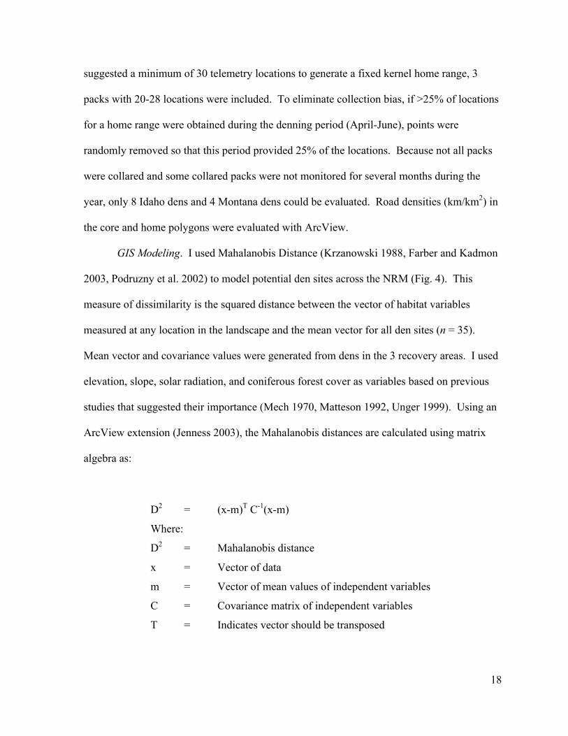
GIS Modeling. I used Mahalanobis Distance (Krzanowski 1988, Farber and Kadmon

2003, Podruzny et al. 2002) to model potential den sites across the NRM (Fig. 4). This

measure of dissimilarity is the squared distance between the vector of habitat variables

measured at any location in the landscape and the mean vector for all den sites (n = 35).

Mean vector and covariance values were generated from dens in the 3 recovery areas. I used

elevation, slope, solar radiation, and coniferous forest cover as variables based on previous

studies that suggested their importance (Mech 1970, Matteson 1992, Unger 1999). Using an

ArcView extension (Jenness 2003), the Mahalanobis distances are calculated using matrix

algebra as:

D2 = (x-m)T C-1(x-m)

Where:

D2 = Mahalanobis distance

x = Vector of data

m = Vector of mean values of independent variables

C = Covariance matrix of independent variables

T = Indicates vector should be transposed

19

Figure 4. Area included for Mahalanobis analysis with densused to generate mean vector and covariance data.

Wolf Dens

20

Because Mahalanobis distances have no upper limit, the values were converted to X2

P-values where P-values close to 0 reflect a high Mahalanobis distance and high dissimilarity

to observed den habitat. P-values close to 1 are similar to den sites. Each threshold P-value

defines a habitat model. I evaluated models by calculating the percentage of wolf dens and

percentage of the landscape that exceeded various threshold P-values. I considered a model

helpful if it encompassed >85% of dens within suitable habitat that comprised < 25% of the

landscape.

21

RESULTS

Wolf Den Characteristics and Fine-scale Habitat Selection

Den Characteristics. Twenty three of 25 dens were hillside excavations with an

average slope of 26.9 + 16.1 (SD) % (Fig. 5). Twelve of the hillside excavations were

categorized as “open,” since they were not directly under a tree; ten were under trees, and

one was under a downed tree. One den was inside a fallen 200+ year old western red cedar

(Thuja plicata). The cedar had suffered from a fire more than one hundred years ago and

eventually fell. The core of the tree was hollow and extended back over 8 meters. Another

den was in the base of an old-growth subalpine fir snag, Abies lasiocarpa, with 61.5”

diameter at breast height. Based on telemetry locations and wolf sign one den area in

Montana was in a forested wetland. In this case, the natal den could not be pinpointed

because there were 5 excavations within 120 m, all of which appeared to be expanded beaver

lodges.

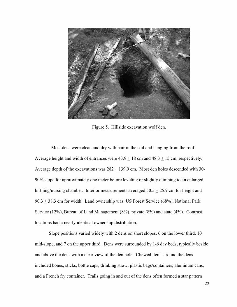
22

Figure 5. Hillside excavation wolf den.

Most dens were clean and dry with hair in the soil and hanging from the roof.

Average height and width of entrances were 43.9 + 18 cm and 48.3 + 15 cm, respectively.

Average depth of the excavations was 282 + 139.9 cm. Most den holes descended with 30-

90% slope for approximately one meter before leveling or slightly climbing to an enlarged

birthing/nursing chamber. Interior measurements averaged 50.5 + 25.9 cm for height and

90.3 + 38.3 cm for width. Land ownership was: US Forest Service (68%), National Park

Service (12%), Bureau of Land Management (8%), private (8%) and state (4%). Contrast

locations had a nearly identical ownership distribution.

Slope positions varied widely with 2 dens on short slopes, 6 on the lower third, 10

mid-slope, and 7 on the upper third. Dens were surrounded by 1-6 day beds, typically beside

and above the dens with a clear view of the den hole. Chewed items around the dens

included bones, sticks, bottle caps, drinking straw, plastic bags/containers, aluminum cans,

and a French fry container. Trails going in and out of the dens often formed a star pattern

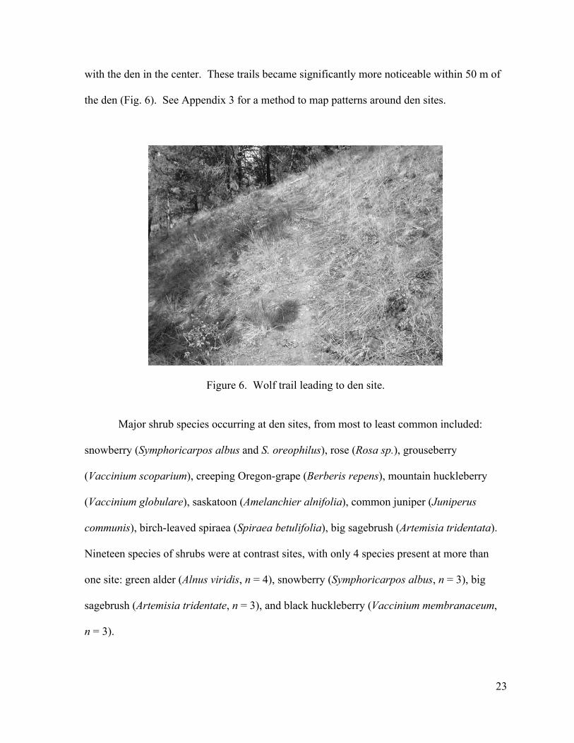
23

with the den in the center. These trails became significantly more noticeable within 50 m of

the den (Fig. 6). See Appendix 3 for a method to map patterns around den sites.

Figure 6. Wolf trail leading to den site.

Major shrub species occurring at den sites, from most to least common included:

snowberry (Symphoricarpos albus and S. oreophilus), rose (Rosa sp.), grouseberry

(Vaccinium scoparium), creeping Oregon-grape (Berberis repens), mountain huckleberry

(Vaccinium globulare), saskatoon (Amelanchier alnifolia), common juniper (Juniperus

communis), birch-leaved spiraea (Spiraea betulifolia), big sagebrush (Artemisia tridentata).

Nineteen species of shrubs were at contrast sites, with only 4 species present at more than

one site: green alder (Alnus viridis, n = 4), snowberry (Symphoricarpos albus, n = 3), big

sagebrush (Artemisia tridentate, n = 3), and black huckleberry (Vaccinium membranaceum,

n = 3).

24

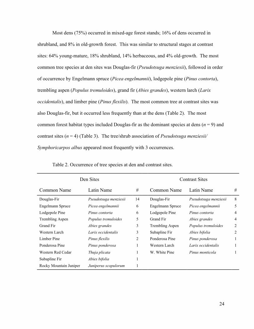
Most dens (75%) occurred in mixed-age forest stands; 16% of dens occurred in

shrubland, and 8% in old-growth forest. This was similar to structural stages at contrast

sites: 64% young-mature, 18% shrubland, 14% herbaceous, and 4% old-growth. The most

common tree species at den sites was Douglas-fir (Pseudotsuga menziesii), followed in order

of occurrence by Engelmann spruce (Picea engelmannii), lodgepole pine (Pinus contorta),

trembling aspen (Populus tremuloides), grand fir (Abies grandes), western larch (Larix

occidentalis), and limber pine (Pinus flexilis). The most common tree at contrast sites was

also Douglas-fir, but it occurred less frequently than at the dens (Table 2). The most

common forest habitat types included Douglas-fir as the dominant species at dens (n = 9) and

contrast sites (n = 4) (Table 3). The tree/shrub association of Pseudotsuga menziesii/

Symphoricarpos albus appeared most frequently with 3 occurrences.

Table 2. Occurrence of tree species at den and contrast sites.

Den Sites Contrast Sites

Common Name Latin Name # Common Name Latin Name #

Douglas-Fir Pseudotsuga menziesii 14 Douglas-Fir Pseudotsuga menziesii 8

Engelmann Spruce Picea engelmannii 6 Engelmann Spruce Picea engelmannii 5

Lodgepole Pine Pinus contorta 6 Lodgepole Pine Pinus contorta 4

Trembling Aspen Populus tremuloides 5 Grand Fir Abies grandes 4

Grand Fir Abies grandes 3 Trembling Aspen Populus tremuloides 2

Western Larch Larix occidentalis 3 Subapline Fir Abies bifolia 2

Limber Pine Pinus flexilis 2 Ponderosa Pine Pinus ponderosa 1

Ponderosa Pine Pinus ponderosa 1 Western Larch Larix occidentalis 1

Western Red Cedar Thuja plicata 1 W. White Pine Pinus monticola 1

Subapline Fir Abies bifolia 1

Rocky Mountain Juniper Juniperus scopulorum 1

25

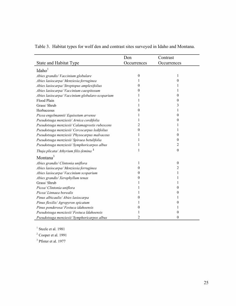
Table 3. Habitat types for wolf den and contrast sites surveyed in Idaho and Montana.

State and Habitat TypeDenOccurrences

ContrastOccurrences

Idaho1

Abies grandis/ Vaccinium globulare 0 1Abies lasiocarpa/ Menziesia ferruginea 1 0Abies lasiocarpa/ Streptopus amplexifolius 0 1Abies lasiocarpa/ Vaccinium caespitosum 0 1Abies lasiocarpa/ Vaccinium globulare-scoparium 1 0Flood Plain 1 0Grass/ Shrub 1 3Herbaceous 0 1Picea engelmannii/ Equisetum arvense 1 0Pseudotsuga menziesii/ Arnica cordifolia 1 0Pseudotsuga menziesii/ Calamagrostis rubescens 2 1Pseudotsuga menziesii/ Cercocarpus ledifolius 0 1Pseudotsuga menziesii/ Physocarpus malvaceus 1 0Pseudotsuga menziesii/ Spiraea betulifolia 1 0Pseudotsuga menziesii/ Symphoricarpos albus 1 2

Thuja plicata/ Athyrium filix-femina 2 1 0

Montana3

Abies grandis/ Clintonia uniflora 1 0Abies lasiocarpa/ Menziesia ferruginea 0 2Abies lasiocarpa/ Vaccinium scoparium 0 1Abies grandis/ Xerophyllum tenax 0 1Grass/ Shrub 1 1Picea/ Clintonia uniflora 1 0Picea/ Linnaea borealis 1 0Pinus albicaulis/ Abies lasiocarpa 0 1Pinus flexilis/ Agropyron spicatum 1 0Pinus ponderosa/ Festuca idahoensis 0 1Pseudotsuga menziesii/ Festuca Idahoensis 1 0

Pseudotsuga menziesii/ Symphoricarpos albus 2 0

1 Steele et al. 19812 Cooper et al. 19913 Pfister et al. 1977

26

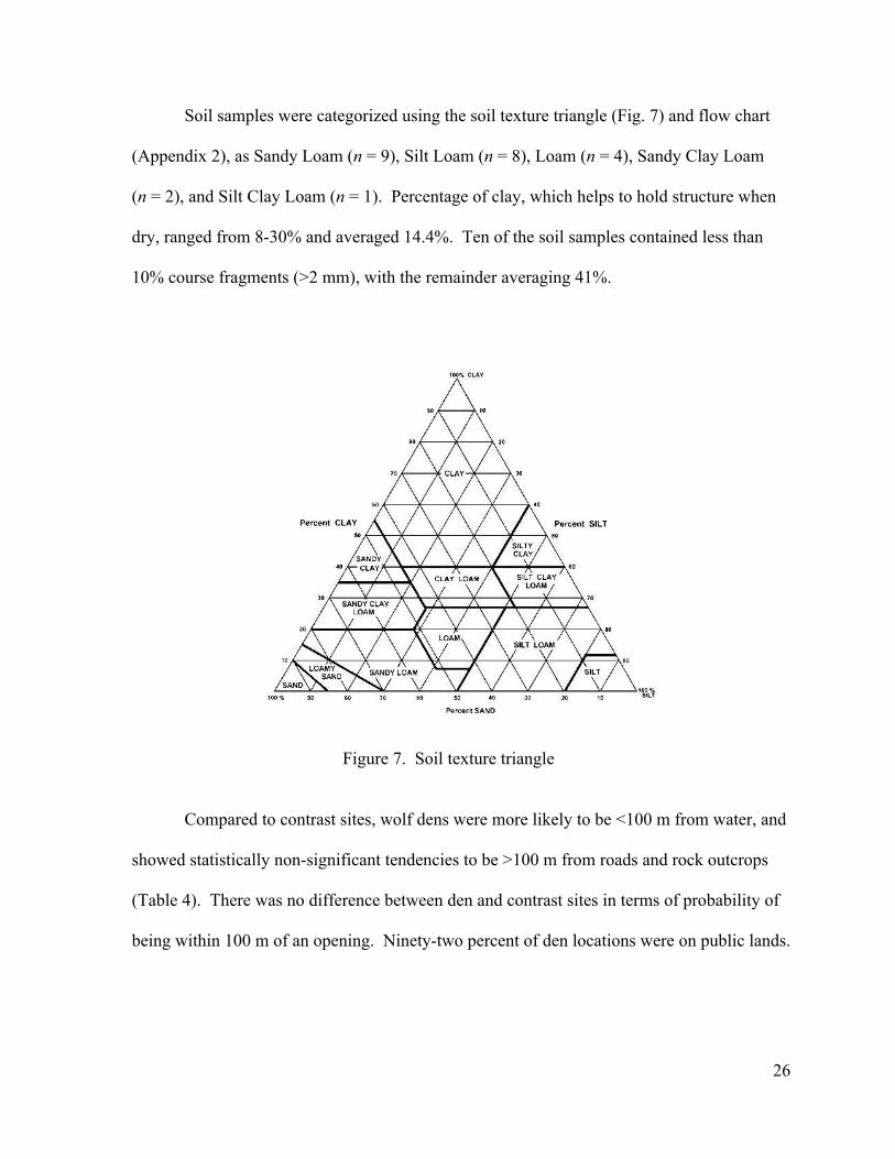
Soil samples were categorized using the soil texture triangle (Fig. 7) and flow chart

(Appendix 2), as Sandy Loam (n = 9), Silt Loam (n = 8), Loam (n = 4), Sandy Clay Loam

(n = 2), and Silt Clay Loam (n = 1). Percentage of clay, which helps to hold structure when

dry, ranged from 8-30% and averaged 14.4%. Ten of the soil samples contained less than

10% course fragments (>2 mm), with the remainder averaging 41%.

Figure 7. Soil texture triangle

Compared to contrast sites, wolf dens were more likely to be <100 m from water, and

showed statistically non-significant tendencies to be >100 m from roads and rock outcrops

(Table 4). There was no difference between den and contrast sites in terms of probability of

being within 100 m of an opening. Ninety-two percent of den locations were on public lands.

27

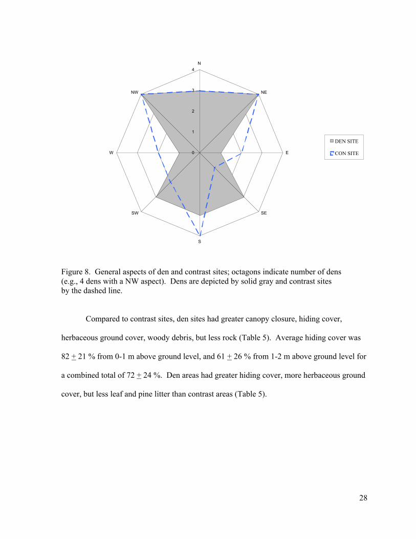
The general aspects of den sites, as well as contrast sites, displayed no significant

pattern (Fig. 8). Eleven dens faced generally North, while 9 of the dens faced generally

South. In most cases (n = 16, 73%) the den opening aspect was within 20 degrees of the

general aspect.

Table 4. Number of sites (out of 22 den sites and 22 contrast sites) within 100 m of variousfeatures. P-value is that of a Chi-squared test of a 2x2 contingency table. Significant values(α = 0.05) are bolded.

FeatureNumber ofden sites

NotesNumber of

contrastsites

Notes P

Water 15 7 .017

Road/Trail 5 4x4 road (3),ATV trail (1),footpath (1)

9 4x4 road (3), ATV trail(2), footpath (2), majorhighway (1), closed dirtroad (1)

.17

Meadow/Opening 11 Meadow (5),sagebrush (4),clear cuts (2)

10 sage brush (3), clearcuts (3), scree/rock (2),grassland (2)

.5

HumanDisturbance

0 3 active logging, highway,active ATV course

.12

Rock Outcrop 2 7 .066

28

0

1

2

3

4

N

NE

E

SE

S

SW

W

NW

DEN SITE

CON SITE

Figure 8. General aspects of den and contrast sites; octagons indicate number of dens(e.g., 4 dens with a NW aspect). Dens are depicted by solid gray and contrast sitesby the dashed line.

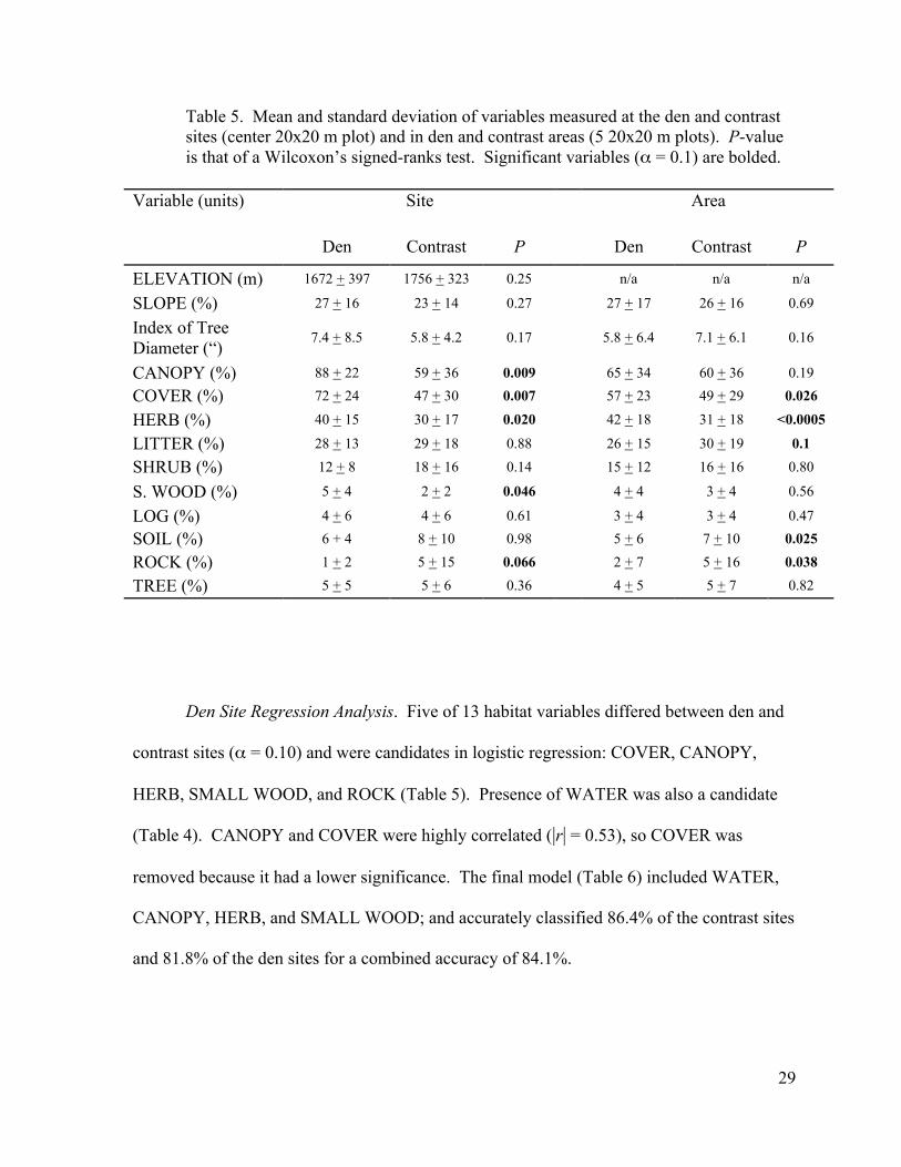
Compared to contrast sites, den sites had greater canopy closure, hiding cover,

herbaceous ground cover, woody debris, but less rock (Table 5). Average hiding cover was

82 + 21 % from 0-1 m above ground level, and 61 + 26 % from 1-2 m above ground level for

a combined total of 72 + 24 %. Den areas had greater hiding cover, more herbaceous ground

cover, but less leaf and pine litter than contrast areas (Table 5).

29

Table 5. Mean and standard deviation of variables measured at the den and contrastsites (center 20x20 m plot) and in den and contrast areas (5 20x20 m plots). P-valueis that of a Wilcoxon’s signed-ranks test. Significant variables (α = 0.1) are bolded.

Variable (units) Site Area

Den Contrast P Den Contrast P

ELEVATION (m) 1672 + 397 1756 + 323 0.25 n/a n/a n/a

SLOPE (%) 27 + 16 23 + 14 0.27 27 + 17 26 + 16 0.69

Index of TreeDiameter (“)

7.4 + 8.5 5.8 + 4.2 0.17 5.8 + 6.4 7.1 + 6.1 0.16

CANOPY (%) 88 + 22 59 + 36 0.009 65 + 34 60 + 36 0.19

COVER (%) 72 + 24 47 + 30 0.007 57 + 23 49 + 29 0.026

HERB (%) 40 + 15 30 + 17 0.020 42 + 18 31 + 18 <0.0005

LITTER (%) 28 + 13 29 + 18 0.88 26 + 15 30 + 19 0.1

SHRUB (%) 12 + 8 18 + 16 0.14 15 + 12 16 + 16 0.80

S. WOOD (%) 5 + 4 2 + 2 0.046 4 + 4 3 + 4 0.56

LOG (%) 4 + 6 4 + 6 0.61 3 + 4 3 + 4 0.47

SOIL (%) 6 + 4 8 + 10 0.98 5 + 6 7 + 10 0.025

ROCK (%) 1 + 2 5 + 15 0.066 2 + 7 5 + 16 0.038

TREE (%) 5 + 5 5 + 6 0.36 4 + 5 5 + 7 0.82

Den Site Regression Analysis. Five of 13 habitat variables differed between den and

contrast sites (α = 0.10) and were candidates in logistic regression: COVER, CANOPY,

HERB, SMALL WOOD, and ROCK (Table 5). Presence of WATER was also a candidate

(Table 4). CANOPY and COVER were highly correlated (|r| = 0.53), so COVER was

removed because it had a lower significance. The final model (Table 6) included WATER,

CANOPY, HERB, and SMALL WOOD; and accurately classified 86.4% of the contrast sites

and 81.8% of the den sites for a combined accuracy of 84.1%.

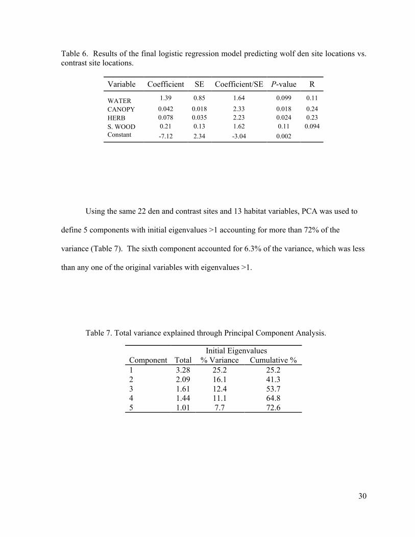
30

Table 6. Results of the final logistic regression model predicting wolf den site locations vs.contrast site locations.

Variable Coefficient SE Coefficient/SE P-value R

WATER 1.39 0.85 1.64 0.099 0.11

CANOPY 0.042 0.018 2.33 0.018 0.24HERB 0.078 0.035 2.23 0.024 0.23S. WOOD 0.21 0.13 1.62 0.11 0.094Constant -7.12 2.34 -3.04 0.002

Using the same 22 den and contrast sites and 13 habitat variables, PCA was used to

define 5 components with initial eigenvalues >1 accounting for more than 72% of the

variance (Table 7). The sixth component accounted for 6.3% of the variance, which was less

than any one of the original variables with eigenvalues >1.

Table 7. Total variance explained through Principal Component Analysis.

Initial EigenvaluesComponent Total % Variance Cumulative %1 3.28 25.2 25.22 2.09 16.1 41.33 1.61 12.4 53.74 1.44 11.1 64.85 1.01 7.7 72.6

31

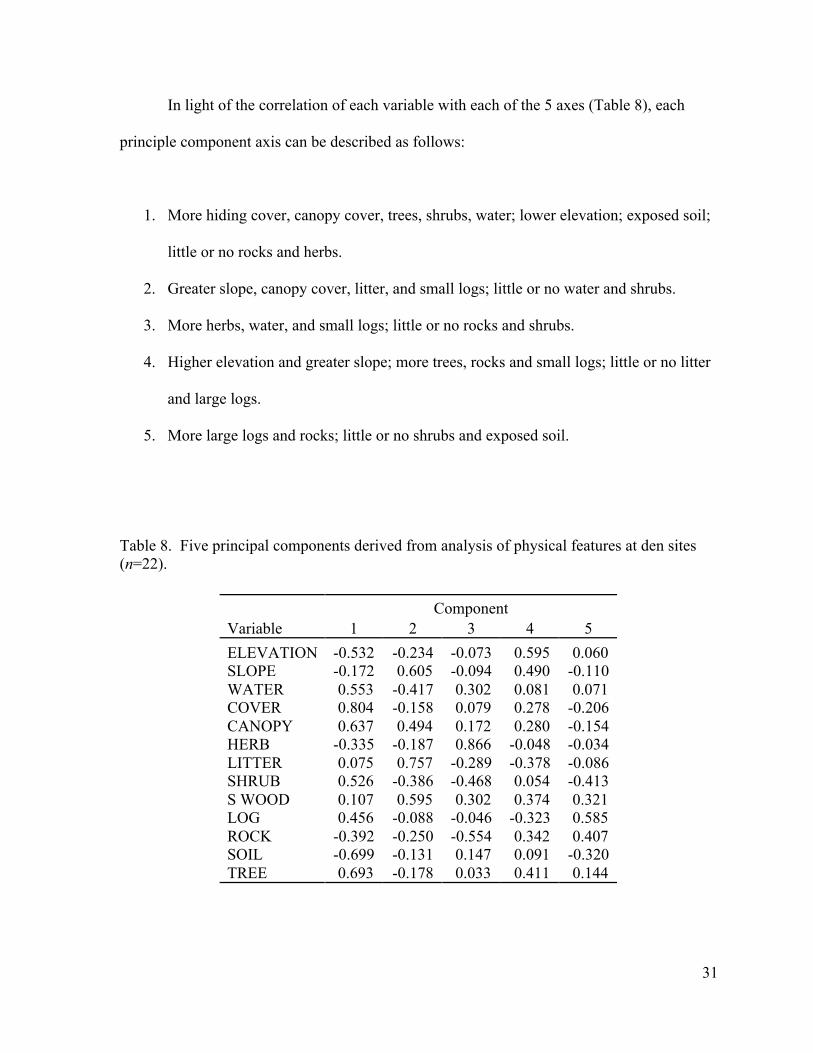
In light of the correlation of each variable with each of the 5 axes (Table 8), each

principle component axis can be described as follows:

1. More hiding cover, canopy cover, trees, shrubs, water; lower elevation; exposed soil;

little or no rocks and herbs.

2. Greater slope, canopy cover, litter, and small logs; little or no water and shrubs.

3. More herbs, water, and small logs; little or no rocks and shrubs.

4. Higher elevation and greater slope; more trees, rocks and small logs; little or no litter

and large logs.

5. More large logs and rocks; little or no shrubs and exposed soil.

Table 8. Five principal components derived from analysis of physical features at den sites(n=22).

ComponentVariable 1 2 3 4 5

ELEVATION -0.532 -0.234 -0.073 0.595 0.060SLOPE -0.172 0.605 -0.094 0.490 -0.110WATER 0.553 -0.417 0.302 0.081 0.071COVER 0.804 -0.158 0.079 0.278 -0.206CANOPY 0.637 0.494 0.172 0.280 -0.154HERB -0.335 -0.187 0.866 -0.048 -0.034LITTER 0.075 0.757 -0.289 -0.378 -0.086SHRUB 0.526 -0.386 -0.468 0.054 -0.413S WOOD 0.107 0.595 0.302 0.374 0.321LOG 0.456 -0.088 -0.046 -0.323 0.585ROCK -0.392 -0.250 -0.554 0.342 0.407SOIL -0.699 -0.131 0.147 0.091 -0.320TREE 0.693 -0.178 0.033 0.411 0.144

32

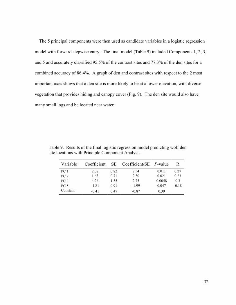
The 5 principal components were then used as candidate variables in a logistic regression

model with forward stepwise entry. The final model (Table 9) included Components 1, 2, 3,

and 5 and accurately classified 95.5% of the contrast sites and 77.3% of the den sites for a

combined accuracy of 86.4%. A graph of den and contrast sites with respect to the 2 most

important axes shows that a den site is more likely to be at a lower elevation, with diverse

vegetation that provides hiding and canopy cover (Fig. 9). The den site would also have

many small logs and be located near water.

Table 9. Results of the final logistic regression model predicting wolf densite locations with Principle Component Analysis

Variable Coefficient SE Coefficient/SE P-value R

PC 1 2.08 0.82 2.54 0.011 0.27PC 2 1.63 0.71 2.30 0.021 0.23PC 3 4.26 1.55 2.75 0.0058 0.3PC 5 -1.81 0.91 -1.99 0.047 -0.18Constant -0.41 0.47 -0.87 0.39

33

Figure 9. Plot of principal component 3 (corresponding to increasing herbaceouscover and small logs, greater probability of water within 100m, and fewer rocksand shrubs) and principal component 1 (corresponding to more hiding cover,canopy cover, trees, shrubs, water; lower elevation, and exposed soil).

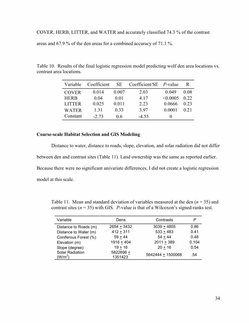
Den Area Regression Analysis. The same variables were examined with the

exception of ELEVATION, which was only recorded at the site (center plot). After

univariate analysis (Wilcoxon’s signed-ranks test) of the 12 habitat variables, 6 showed

significance (α = 0.10) and were retained: WATER, COVER, HERB, LITTER, SOIL and

ROCK, none of which exhibited multicollinearity. The final model (Table 10) included

Principle Component 1

210-1-2-3

Prin

cipl

e C

ompo

nent

3

2

1

0

-1

-2

-3

-4

Data

Dens

Random

Total Population

34

COVER, HERB, LITTER, and WATER and accurately classified 74.3 % of the contrast

areas and 67.9 % of the den areas for a combined accuracy of 71.1 %.

Table 10. Results of the final logistic regression model predicting wolf den area locations vs.contrast area locations.

Variable Coefficient SE Coefficient/SE P-value R

COVER 0.014 0.007 2.03 0.049 0.08HERB 0.04 0.01 4.17 <0.0005 0.22LITTER 0.025 0.011 2.23 0.0666 0.23WATER 1.31 0.33 3.97 0.0001 0.21Constant -2.73 0.6 -4.55 0

Coarse-scale Habitat Selection and GIS Modeling

Distance to water, distance to roads, slope, elevation, and solar radiation did not differ

between den and contrast sites (Table 11). Land ownership was the same as reported earlier.

Because there were no significant univariate differences, I did not create a logistic regression

model at this scale.

Table 11. Mean and standard deviation of variables measured at the den (n = 35) andcontrast sites (n = 35) with GIS. P-value is that of a Wilcoxon’s signed-ranks test.

Variable Dens Contrasts P

Distance to Roads (m) 2654 + 3432 3039 + 4855 0.86Distance to Water (m) 412 + 311 533 + 483 0.41Coniferous Forest (%) 59 + 44 54 + 44 0.48Elevation (m) 1916 + 404 2011 + 389 0.104Slope (degree) 19 + 16 20 + 16 0.54Solar Radiation(W/m2)

5822696 +1351423

5642444 + 1500068 .54

35

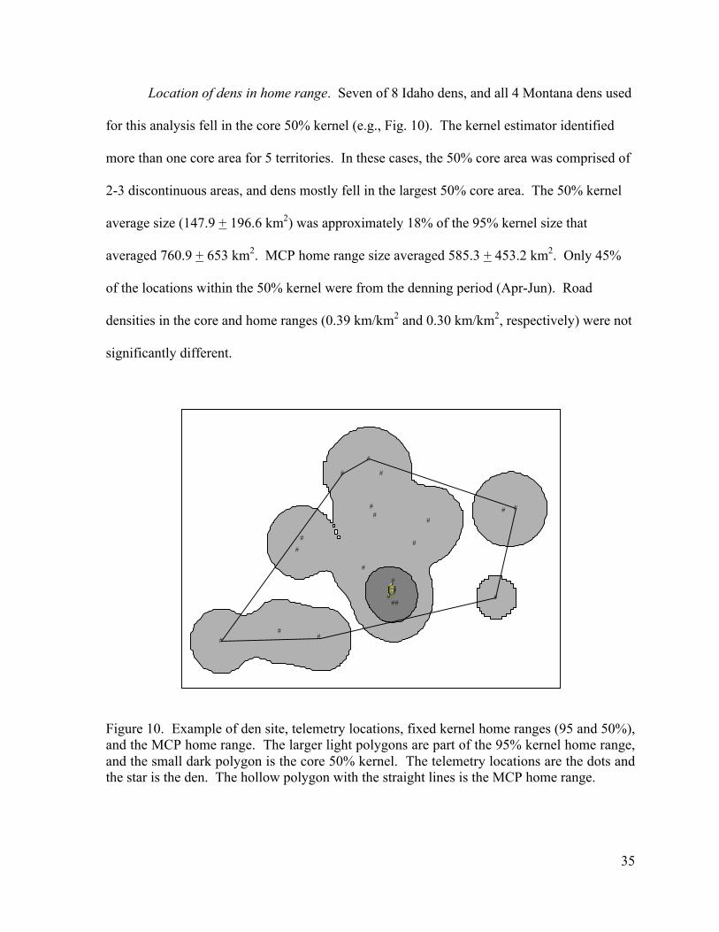
Location of dens in home range. Seven of 8 Idaho dens, and all 4 Montana dens used

for this analysis fell in the core 50% kernel (e.g., Fig. 10). The kernel estimator identified

more than one core area for 5 territories. In these cases, the 50% core area was comprised of

2-3 discontinuous areas, and dens mostly fell in the largest 50% core area. The 50% kernel

average size (147.9 + 196.6 km2) was approximately 18% of the 95% kernel size that

averaged 760.9 + 653 km2. MCP home range size averaged 585.3 + 453.2 km2. Only 45%

of the locations within the 50% kernel were from the denning period (Apr-Jun). Road

densities in the core and home ranges (0.39 km/km2 and 0.30 km/km2, respectively) were not

significantly different.

Figure 10. Example of den site, telemetry locations, fixed kernel home ranges (95 and 50%),and the MCP home range. The larger light polygons are part of the 95% kernel home range,and the small dark polygon is the core 50% kernel. The telemetry locations are the dots andthe star is the den. The hollow polygon with the straight lines is the MCP home range.

#

##

#

#

#

#

#

#

##

#

#

##

#

#

#

##

#

ÊÚ

36

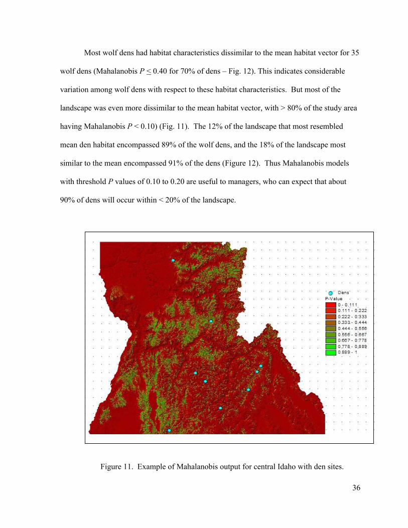
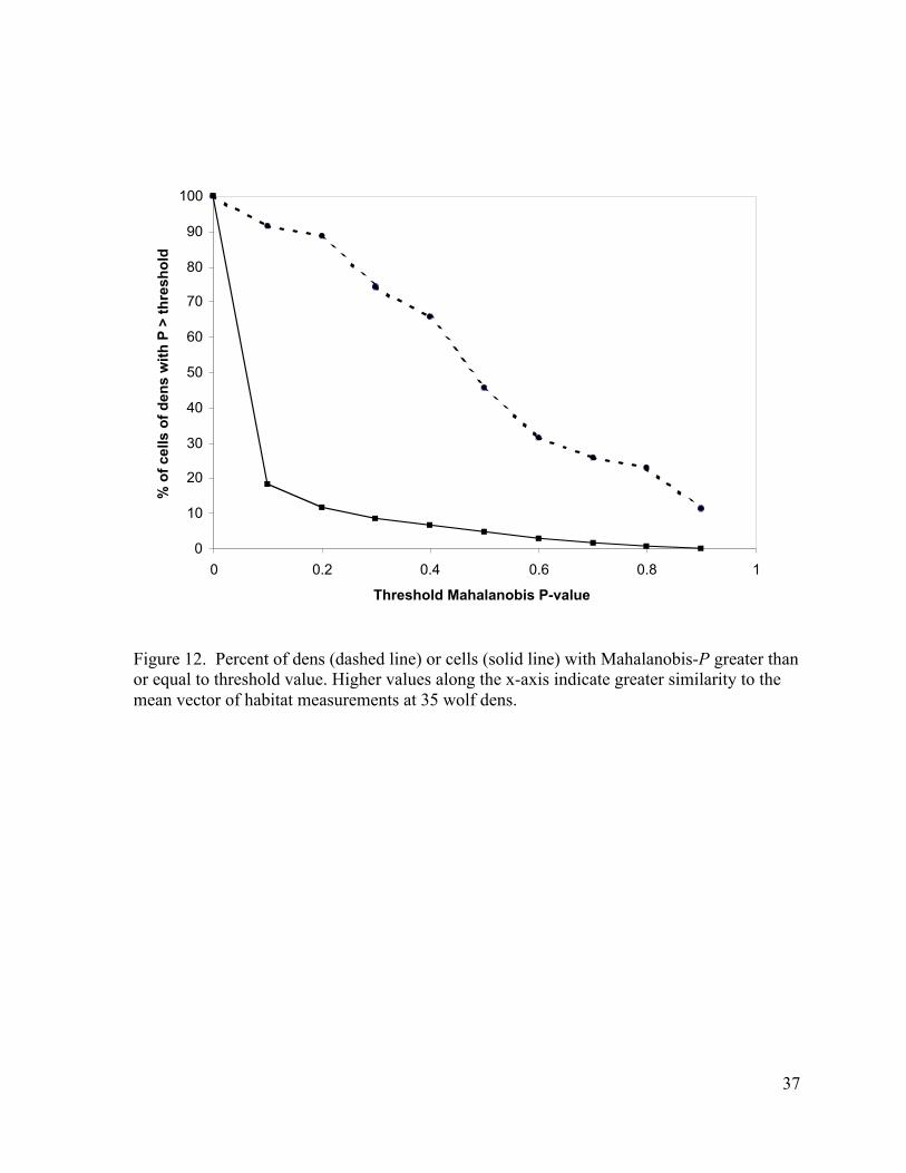
Most wolf dens had habitat characteristics dissimilar to the mean habitat vector for 35

wolf dens (Mahalanobis P < 0.40 for 70% of dens – Fig. 12). This indicates considerable

variation among wolf dens with respect to these habitat characteristics. But most of the

landscape was even more dissimilar to the mean habitat vector, with > 80% of the study area

having Mahalanobis P < 0.10) (Fig. 11). The 12% of the landscape that most resembled

mean den habitat encompassed 89% of the wolf dens, and the 18% of the landscape most

similar to the mean encompassed 91% of the dens (Figure 12). Thus Mahalanobis models

with threshold P values of 0.10 to 0.20 are useful to managers, who can expect that about

90% of dens will occur within < 20% of the landscape.

Figure 11. Example of Mahalanobis output for central Idaho with den sites.

37

0

10

20

30

40

50

60

70

80

90

100

0 0.2 0.4 0.6 0.8 1

Threshold Mahalanobis P-value

% o

f ce

lls o

f d

ens

wit

h P

> t

hre

sho

ld

Figure 12. Percent of dens (dashed line) or cells (solid line) with Mahalanobis-P greater thanor equal to threshold value. Higher values along the x-axis indicate greater similarity to themean vector of habitat measurements at 35 wolf dens.

38

DISCUSSION

Although both univariate and multivariate techniques are commonly used to describe

habitat selection, the univariate methods (e.g., Wilcoxon’s signed-ranks test) can fail to

address confounding of highly correlated variables. The removal of hiding cover from the

regression analysis due to its correlation with canopy cover to be problematic. Both canopy

and hiding cover were highly significant. PCA eliminated the problem of covariance, but

produced a characterization of dens that was not as clearly related to the measured habitat

variables. Each of the 13 habitat variables were significant in at least 2 of the 5 principal

components. Overall, univariate and multivariate techniques produced similar results and

suggest that water within 100 m, canopy cover, herbaceous ground cover, small logs, and

rocks are the most important factors influencing selection of den sites at the fine-scale.

Finding den sites near water was an expected outcome. Dens are often near water,

probably due to the lactating female’s increased need for hydration (Mech 1970; Peterson

1977, Norris et al. 2002). In south-central Alaska, Ballard and Dau (1983) found the average

distance from den sites to a water source was 257 + 263 meters.

I found dense cover near dens, which is consistent with the fact that dens were often

difficult to find and could rarely be seen from >20 meters. Previous studies in Montana

(Matteson 1992) and Wisconsin-Minnesota (Unger 1999) did not find a significant cover

difference between den and contrast locations. Matteson (1992) measured cover at 30.5 and

61 m (compared to 15 m in this study); at these distances, Matteson found dense cover values

at dens with 66.1 + 27.3% and 91 + 17.3, respectively. I believe Matteson measured cover at

inappropriately long distances from the center of den and contrast sites, which could have

reduced the power to detect differences. Unger (1999) collected data at 16 m, but used a 1 m

39

high cover board compared to the 2-m cover pole used in this study. Unger (1999) found

average hiding cover at dens to be 70 + 24%, which is comparable to my results (72 + 24%).

Perhaps the vegetative structure in northwest Wisconsin and east-central Minnesota is not as

diverse and more dense than in the NRM.

Canopy cover was also considered to be insignificant by Matteson (1992) and Unger

(1999). The average canopy cover reported by Unger (1999) was 43.3 + 8.8%, and 18.9 +

21.3% by Matteson (1992), which is much less than the 87.6 + 21.8% I observed. These

differences could be explained by the different collection methods. Matteson (1992) visually

estimated canopy cover whereas Unger (1999) used a point-intercept method. Nuttle (1997)

suggested that point-intercept methods may not reflect an animal’s perception of canopy

cover. Although Matteson’s study did not show statistical significance for canopy and hiding

cover, she believed they played an important role within a 100-m radius of the den.

My fine-scale analysis did not identify elevation as an important variable. However,

Matteson (1992) found dens at lower elevation than contrast locations, and called elevation

the “overriding factor” for den site selection. Matteson (1992) found an average elevation of

1352 + 221 m at dens, compared to my mean of 1672 + 397. However, mean elevation was

1209 + 176 m) for the subset of my dens that fall in Matteson’s (1992) study area (i.e.,

northwest Montana and southern Canada). In my study average elevations were 1216 + 170

m and 2065 + 240 m north and south of the 46th parallel, respectively. Stephenson (1974)

found an average elevation of 635 m for dens in the Brooks Range of Alaska. While these

data suggest a trend, additional research would be required to determine if wolves are

actually selecting lower elevations for den sites at higher latitudes and vice versa.

40

Unger (1999) found steeper slopes at dens versus contrast sites. Although I did not

identify slope as a selected den site attribute, my average slope of 27% was similar to

Unger’s 25% (1999). Matteson (1992) found average slopes of 16 + 19%. Stephenson

(1974) found a much higher average slope of 65% in the Brooks Range of Alaska. Using

elevation and slope measured in a GIS, Oakleaf (2002) found core areas of pack home ranges

in the NRM at lower elevations with gentler slopes. While I found that most dens were

located within home range core areas, I found no significant correlation between den sites

and elevation or slope.

Variables that displayed significance at both site and area scale included hiding cover,

herbaceous ground cover, and rock cover. At the area scale increased bare soil at the contrast

locations was significantly different from the dens. Increased canopy cover and small woody

debris was significant at the site level, suggesting that wolves respond to these 2 factors only

in the area immediately surrounding the den hole. The increased canopy cover at the den

hole could suggest that wolves select an area with more vertical protection, or this could be

an artifact of site selection near tree roots for increased structural integrity. Although small

woody material may provide little structural defense from ground predators, it may provide

visual obscurity. Golden Eagles (Aquila chrysaetos) have been known to take fox (Vulpes

vulpes) pups nears den sites (C. McIntyre, personal communication), so it is possible that

woody debris and canopy cover may provide some protection from raptors.

Approximately half of the dens in my study were associated with trees and their root

systems. This is consistent with Matteson’s (1992) results of 8 of 15 dens at the base of

trees, framed by roots. Perhaps den selection under trees and in their root structure is

particular to wolves in the Northern Rockies. My measurements of den size and shape were

41

similar to previous studies. Most dens had distinct, enlarged terminal chambers, consistent

with the findings of Ballard and Dau (1983). However, Unger (1999) did not find dens with

distinct birthing chambers. I found soil composition similar to that in previous studies.

Wolves usually dig dens in stable, sandy soil, probably due to easy digging and good

drainage (Mech 1970, Peterson 1977; Ballard and Dau 1983; Unger 1999). Matteson (1992)

found the most frequent texture type to be loam.

Wolves apparently did not select any one aspect for den sites. Unger (1999) found

similar results, but Matteson (1992) found a moderate preference by wolves for south and

east facing slopes. Solar radiation at dens does not appear to be a factor in selection.

Unger (1999) called the area within 50 m of the den a “heavy use” area. I also found

a significant increase in sign (e.g., day beds, scats, trails) within 50 m of the den. Wolf trails

were characterized by their width and “softness,” as compared to ungulate trails which are

often more “harsh” because of their sharp hooves. J. Young and M. Elbroch (Shikari

Tracking Guild, unpublished data, Appendix 3) measured direct register trot impressions in

the trails and calculated a stride length of 28 inches, similar to Elbroch’s (2003) range of 22-

34”, with a trail width of 4-9_”. Tracks and other sign around the dens can help to determine

how recently a den was used and differentiate between wolf and other canid dens.

Road and water GIS layers at the 1:100,000 resolution were inaccurate. In the field, I

found most dens to be within 100 m of water, although GIS data only revealed 3 water

sources within that distance. Several roads were depicted as within 30 m of dens, but I found

no such roads in the field. These inaccuracies probably contributed to the lack of significant

differences (Table 11) and my inability to construct a coarse-scale model of den selection.

42

Eleven of 12 den locations tested fell within the core home range (50% fixed kernel)

polygon. Unger (1999) found that dens tended to be in the central part of the MCP, but

Ciucci and Mech (1992) found wolf dens located randomly throughout the MCP home

ranges. However, these findings could be a result of different methods in the analysis.

Ciucci and Mech (1992) examined wolf den locations by calculating the mean radius for each

territory as the average of the radii from the center to the vertices of the polygon. Unger

(1999) characterized the core area by simply reducing the same dimensions of the 100%

MCP by 75%. Both of these studies examined den location as either being centrally or

peripherally located in the MCP home range. Fifty percent fixed kernel estimators examine

the intensity of use in the home range, and therefore are a better predictor of denning areas.

In my study only 45% of the locations within the 50% kernel were from the denning

period (Apr-Jun). This supports the theory that wolves use the denning area throughout the

year. Road densities were not significantly different between core and home range kernels,

which is consistent with Oakleaf’s (2002) results.

Although there was considerable variation among wolf dens with respect to elevation,

slope, solar radiation, and coniferous forest cover, I identified several useful Mahalanobis

distance models using these GIS data layers. By combining Mahalanobis modeling with

fixed kernel home ranges and core use areas, potential denning habitat can be identified.

43

CONCLUSIONS AND MANAGEMENT IMPLICATIONS

Den site selection appears strongest within about 15 m of the den hole, but was also

apparent (but less pronounced) within a 50-m radius of the den. That den sites had more

hiding cover, canopy cover, and woody debris than random sites suggests that wolves select

denning habitat for its added protective value. The den structure itself with a narrow tunnel

leading to a larger birthing chamber may also be related to protection. Although elevation

was not found to be significantly different between dens and random contrast locations,

average elevation of dens decreased as latitude increased. Close proximity to water is also a

significant factor. To help standardize den site data collection in the NRM, I have included a

recommended den data collection form (Appendix 4).

More than 90% of the dens fell within the 50% fixed kernel core use area of the pack,

which corresponds to a mean of 147.9 + 196.6 km2. Because these core areas are visited by

the wolves throughout the year, managers may want to consider actions that would limit

human disturbance year round in these areas. One-kilometer closure areas around den sites,

which have been used in the Yellowstone and Mexican wolf (Canis lupus baileyii) recovery

areas, may be too small to adequately protect wolves from detrimental effects of human

disturbance. The 50% kernel would be a better closure perimeter for 2 reasons: 1) it

represents a less arbitrary boundary of the important wolf area around the dens, and 2) it

makes finding dens by inquisitive citizens more difficult, because the closed area is larger

and dens are often not in the geographic center of the kernel. However, the large closure size

delineated by 50% kernel would not be socially acceptable in many cases. The size and

44

shape of the closures should be contingent on the potential for human disturbance during that

period.

Minimum Convex Polygons are the standard method for delineating wolf home

ranges in the NRM, and several studies have examined den site locations within 100% MCP

home ranges. However, 100% MCP home ranges do not consider intensity of use, which

should be considered when examining core use areas and wolf dens. When managers are

attempting to identify potential core wolf habitat, I recommend the use of the 50% fixed

kernel estimator which accounts for intensity of use.

Once dens are located, efforts could be made to protect these areas from human

disturbance, development, and habitat alterations because wolves often reuse the same den in

subsequent years. Additionally, the core areas should be protected because the availability of

suitable den sites may limit the overall carrying capacity of regional habitats for wolves. If

human disturbance does take place near or in the core areas, managers should monitor to

determine if a shift in the core area takes place over the following year.

Although some GIS-derived data layers were accurate (e.g., elevation, slope, aspect),

other data layers (e.g., roads and water) were highly inaccurate compared to site-specific data

measured in the field. As GIS use becomes more prevalent, managers should be aware of

some of its potential limitations. Layers used in modeling habitat should be sufficiently

accurate for the level of analysis desired.

Mahalanobis models can help managers identify suitable den habitat (defined by P >

0.20). Managers can use these models to limit human disturbance in potential denning areas,

or to evaluate the amount of denning habitat in existing wolf populations or proposed

reintroduction sites. Because 80-90% of dens occur in suitable denning habitat that

45

comprises only 12-18% of the recovery area, denning habitat may be a limiting factor. The

modeling area can be further refined by calculating Mahalanobis distances within pack home

range or core territories.

Further study should be focused on den site location in relation to ungulate

distribution. In the Artic, wolves have located their dens in the migration route of the caribou

(C. Rangifer) (Walton et al. 2001). I would expect to see a pattern emerging in the NRM

with respect to elk calving grounds and ungulate winter and summer ranges. Additionally,

this analysis could also be applied to rendezvous sites. Future research should investigate

whether pup survival is related to den site characteristics, available prey, and human

disturbance.

46

LITERATURE CITED

Ballard WB and Dau JR. 1983. Characteristics of gray wolf, Canis lupus, den and

rendezvous sites in southcentral Alaska. Can Field-Nat 97(3):299-302.

Ballard WB, Whitman JS, Gardner CL. 1987. Ecology of an exploited wolf population in

south-central Alaska. Wildl Mon 98:1-54.

Banfield AWF. 1954. Preliminary investigations of the barren ground caribou. Part 2. Life

history, ecology, and utilization. Canadian Wildlife Service, Wildlife Management Bulletin.

Series 1, No. 10B.

Boertje RD and Stephenson RO. 1992. Effects of ungulate availability on wolf reproductive

potential in Alaska. Can J Zool 70:2441-2443.

Carbyn LN. 1975. Factors influencing activity patterns of ungulates at mineral licks. Can J

Zool 53:378-84.

Carroll C, Phillips M, Schumaker NH, Smith DW. 2003. Impacts of landscape change on

wolf restoration success: planning a reintroduction program based on static and dynamic

spatial models. Con Bio 17(2):536-48.

Ciucci P and Mech LD. 1992. Selection of dens in relation to winter territories in

northeastern Minnesota. J Mamm 73(4):899-905.

Clark JD, Dunn JE, Smith KG. 1993. A multivariate model of female black bear habitat for

a geographic information system. J Wildl Manage 57(3):519- 26.

Cooper SV, Neiman KE, Roberts DW. 1991. Forest habitat types of Northern Idaho. US

Forest Service, Intermountain Research Station. 143 p.

47

Corsi F, Dupre E, Boitani L. 1999. A large-scale model of wolf distribution in Italy for

conservation planning. Con Bio 13(1):150-59.

Elbroch M. 2003. Mammal tracks and sign: a guide to North American species.

Pennsylvania: Stackpole Books. 778 p.

ESRI. 1992. ArcView 3.2. Environmental Systems Research Institute. Redlands, CA.

Farber O and Kadmon R. 2003. Assessment of alternative approaches for bioclimatic

modeling with special emphasis on the Mahalanobis distance. Ecological Modeling 160:

115-30.

Fuller T. 1989. Denning behavior of wolves in north-central Minnesota. Am. Midl. Nat.

121: 184-88.

Garmin TM eTrex Summit. Garmin International, Inc. 1200 E. 151st St. Olathe, Kansas

66062.

Griffith B and Youtie BA. 1988. Two devices for estimating foliage density and deer hiding

cover. Wildl Soc Bull 16:206-10.

Haber GC. 1968. The social structure and behavior of an Alaskan wolf population. MA

thesis. Northern Michigan University , Marquette.

Haight RG, Mladenoff DJ, Wydeven AP. 1998. Modeling disjunct gray wolf populations in

semi-wild landscapes. Con Bio 12(4):879-888.

Harrington FH and Mech LD. 1982. Patterns of homesite attendance in two Minnesota wolf

packs. In: Harrington FH and Paquet PC, editors. Wolves of the world: perspectives of

behavior, ecology, and conservation. New Jersey: Noyes Publications. 474 p.

48

Hayward GD, Hayward PH, Garton EO. 1993. Ecology of boreal owls in the Northern

Rocky Mountains, U.S.A. Wildl Mon 124:1-59.

Hooge PN, Eichenlaub W, Solomon E. 1999. The animal movement program. USGS,

Alaska Biological Science Center, Anchorage, USA.

Hosmer DW and Lemeshow S. 2000. Applied logistic regression. 2nd ed. New York:

Wiley and Sons Inc.

Houts ME. 2001. Modeling gray wolf habitat in the Northern Rocky Mountains. MA

Thesis, University of Kansas. 87 p.

Jenness J. 2003. Mahalanobis distances extension for ArcView 3.x. Jenness Enterprises.

<http://www.jennessent.com/arcview/mahalanobis.htm> [Accessed 3/02/04]

Kershaw L, MacKinnon A, Pojar J. 1998. Plants of the Rocky Mountains. Canada: Lone

Pine. 384 p.

Kolowski JM and Woolf A. 2002. Microhabitat use by bobcats in southern Illinois. J. Wildl

Manage 66(3):822-832.

Krzanowski WJ. 1988. Principles of multivariate analysis. Oxford: Clarendon Press. 563 p.

Lemon PE. 1957. A new instrument for measuring forest overstory density. J Forestry

55(9):667-668.

Maptech. 2002. Terrain Navigator. 10 Industrial Way, Amesbury, MA 01913.

Matteson MY. 1992. Denning ecology of wolves in Northwest Montana and Southern

Canadian Rockies. MS Thesis, University of Montana. 65 p.

49

McLoughlin PD, Walton LR, Cluff HD, Paquet PC, Ramsay PM. 2004. Hierarchical habitat

selection by tundra wolves. J Mamm 85(3):

Mech LD. 1970. The wolf: the ecology and behavior of an endangered species. Minnesota:

University of Minnesota Press. 384 p.

Mech LD. 1989. Wolf population survival in an area of high road density. Am Midl Nat

121:387-389.

Mech LD. 2000. Leadership in wolf, Canis lupus, packs. Can Field-Nat 114:259-63.

Mech LD and Packard JM. 1990. Possible use of wolf, Canis lupus, den over several

centuries. Can. Field-Nat. 104(3): 484-85.

Mech LD, Adams LG, Meier TJ, Burch JW, Dale BW. 1998. The wolves of Denali.

London: University of Minnesota Press. 227 p.

Mech LD, Wolf PC, Packard JM. 1999. Regurgitative food transfer among wild wolves.

Can J Zool 77:1192-1195.

Mladenoff DJ, Sickley TA, Wydeven AP. 1999. Predicting gray wolf landscape

recolonization: logistic regression models vs. new field data. Ecological Applications 9(1):

37-44.

Murie A. 1944. The wolves of Mount McKinley. Fauna of the National Parks of the U.S.

Fauna Series No. 5. 238 p.

Norris DR, Theberge MT, Theberge JB. 2002. Forest composition around wolf dens in

eastern Algonquin Provincial Park, Ontario. Can J Zool 80:866-872.

50

Nuttle T. 1997. Densiometer bias? Are we measuring the forest or the trees? Wildl Soc Bull

25(3):610-611.

Oakleaf JK. 2002. Wolf-cattle interactions and habitat selection by recolonizing wolves in

the northwestern United States. MS Thesis, University of Idaho. 67 p.

Paquet PC and Carbyn LN. 2003. Gray wolf. In: Feldhamer GA, Thompson BC, Chapman

JA, editors. Wild mammals of North America: biology, management, and conservation.

London: Johns Hopkins University Press. p 482-510.

Peterson RO. 1977. Wolf ecology and prey relationships on Isle Royale. National Park

Service Scientific Monograph Series. No. 11. 210 p.

Pfister RD, Kovalchik BL, Arno SF, Presby R. 1977. Forest habitat types of Montana. U.S.

Forest Service, Intermountain Forest and Range Experiment Station. 174 p.

Podruzny SR, Cherry S, Schwartz CC, Landenburger LA. 2002. Grizzly bear denning and

potential conflict areas in the Greater Yellowstone Ecosystem. Ursus 13:19-28.

Powell RA, Zimmerman JW, Seaman DE. 1997. Ecology and behavior of North American

black bears: home ranges, habitat and social organization. London: Chapman and Hall.

Ramsey FL and Schafer DW. 1997. The statistical sleuth. Boston: Duxbury Press. 742 p.

Seaman DE, Millspaugh JJ, Kernohan BJ, Brundige GC, Raedeke KJ, Gitzen RA. 1999.

Effects of sample size on kernel home range estimates. J Wildl Manage 63.

Steele R, Pfister RD, Ryker RA, Kittams JA. 1981. Forest habitat types of central Idaho.

U.S. Forest Service, Intermountain Forest and Range Experiment Station. General Technical

Report INT-114.

51

Thiel RP, Merrill S, Mech LD. 1998. Tolerance by denning wolves, Canis lupus, to human

disturbance. Can Field-Nat 112(2):340-42.

Thien SJ. 1979. A flow diagram for teaching texture-by-feel analysis. J Agronomic

Education 8:54-55.

Thurston LM. 2002. Homesite attendance as a measure of alloparental and parental care by

gray wolves in northern Yellowstone National Park. MS Thesis, Texas A&M. 175 p.

Unger D. 1999. A multi-scale analysis of timber wolf den and rendezvous site selection in

northwestern Wisconsin and east-central Minnesota. MS Thesis, University of Wisconsin-

Stevens Point. 76 p.

U.S. Fish and Wildlife Service. 1987. The Northern Rocky Mountain wolf recovery plan.

U.S. Fish and Wildlife Service, Denver, Colorado. 119 p.

U. S. Fish Wildlife Service, Nez Perce Tribe, National Park Service, USDA Wildlife

Services. 2001. Rocky Mountain wolf recovery 2000 annual report.

U.S. Fish and Wildlife Service, Nez Perce Tribe, National Park Service, USDA Wildlife

Services. 2004. Rocky Mountain wolf recovery 2003 annual report. Meier T, editor.

USFWS, Ecological Services, 100 N Park, Suite 320, Helena MT. 65 p.

U.S. Geological Survey. 2002. Gap analysis final report and data. National Gap Analysis

Office, Moscow, ID.

U.S. Census Bureau. 2002. Topologically Integrated Geographic Encoding and Referencing

System.

Walton LR, Cluff HD, Paquet PC, Ramsay MA. 2001. Movement patterns of barren-ground

wolves in the central Canadian Arctic. J Mamm 82(3):867-876.

52

Wydeven AP, Mladenoff DJ, Sickley TA, Kohn BE, Thiel RP, Hansen JL. 2001. Road

density as a factor in habitat selection by wolves and other carnivores in the Great Lakes

region. Endangered Species Update 18(4):110-14.

Zar JH. 1999. Biostatistical analysis. 4th ed. New Jersey: Prentice Hall. 663 p.

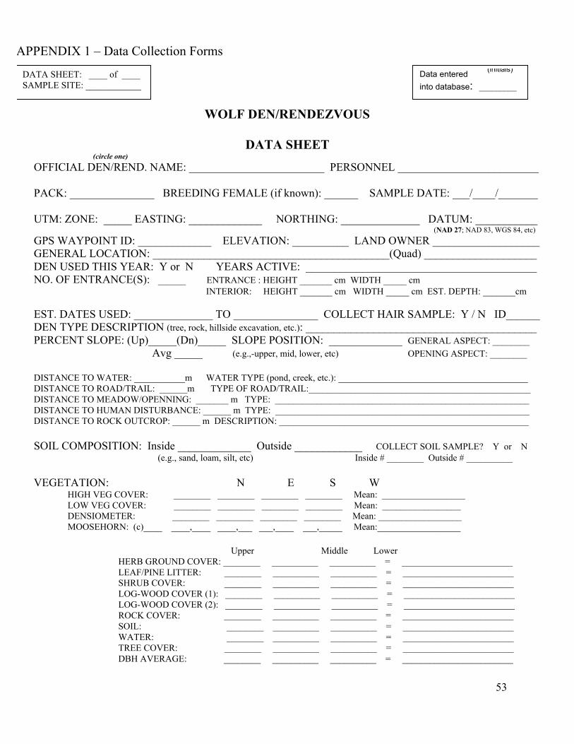
53

WOLF DEN/RENDEZVOUS

DATA SHEET (circle one)

OFFICIAL DEN/REND. NAME: ________________________ PERSONNEL _________________________

PACK: _______________ BREEDING FEMALE (if known): ______ SAMPLE DATE: ___/____/_______

UTM: ZONE: _____ EASTING: _____________ NORTHING: ______________ DATUM: ___________ (NAD 27; NAD 83, WGS 84, etc)

GPS WAYPOINT ID: _____________ ELEVATION: __________ LAND OWNER ___________________GENERAL LOCATION: __________________________________________(Quad) ____________________DEN USED THIS YEAR: Y or N YEARS ACTIVE: _________________________________________NO. OF ENTRANCE(S): ______ ENTRANCE : HEIGHT _______ cm WIDTH _____ cm

INTERIOR: HEIGHT _______ cm WIDTH _____ cm EST. DEPTH: _______cm

EST. DATES USED: ______________ TO _______________ COLLECT HAIR SAMPLE: Y / N ID______DEN TYPE DESCRIPTION (tree, rock, hillside excavation, etc.): _________________________________________PERCENT SLOPE: (Up)_____(Dn)_____ SLOPE POSITION: _____________ GENERAL ASPECT: ________ Avg _____ (e.g.,-upper, mid, lower, etc) OPENING ASPECT: ________

DISTANCE TO WATER: ___________m WATER TYPE (pond, creek, etc.): _________________________________________DISTANCE TO ROAD/TRAIL: ______m TYPE OF ROAD/TRAIL:________________________________________________DISTANCE TO MEADOW/OPENNING: _______ m TYPE: _______________________________________________________DISTANCE TO HUMAN DISTURBANCE: ______ m TYPE: _______________________________________________________DISTANCE TO ROCK OUTCROP: ______ m DESCRIPTION: ______________________________________________________

SOIL COMPOSITION: Inside _____________ Outside ____________ COLLECT SOIL SAMPLE? Y or N (e.g., sand, loam, silt, etc) Inside # ________ Outside # __________

VEGETATION: N E S WHIGH VEG COVER: ________ ________ ________ ________ Mean: __________________

LOW VEG COVER: ________ ________ ________ ________ Mean: _________________DENSIOMETER: ________ ________ ________ ________ Mean: __________________MOOSEHORN: (c)____ ____,____ ____,___ ___,____ ___,_____ Mean:__________________

Upper Middle LowerHERB GROUND COVER: ________ __________ __________ = ________________________LEAF/PINE LITTER: ________ __________ __________ = ________________________SHRUB COVER: ________ __________ __________ = ________________________LOG-WOOD COVER (1): ________ __________ __________ = ________________________LOG-WOOD COVER (2): ________ __________ __________ = ________________________ROCK COVER: ________ __________ __________ = ________________________SOIL: ________ __________ __________ = ________________________WATER: ________ __________ __________ = ________________________TREE COVER: ________ __________ __________ = ________________________DBH AVERAGE: ________ __________ __________ = ________________________

APPENDIX 1 – Data Collection Forms

Data entered(initials)

into database: _________

DATA SHEET: ____ of ____SAMPLE SITE: ____________

54

HABITAT TYPE: ___________________________ STRUCTURAL CLASS: _________________________________________MAJOR TREE SPP: __________________________ MAJOR SHRUB SPP: ____________________________________________DISTANCE TO EDGE: _______ m

PHOTOS TAKEN: Y or N EXPOSURE NUMBERS: FROM ____________ to __________________DIGITAL: Y or N

PREY OBSERVATIONS: ___________________________________________________________________

__________________________________________________________________________________________

ADDITIONAL OBSERVATIONS (Remains, scats, day beds, trails, etc): ______________________________

__________________________________________________________________________________________

__________________________________________________________________________________________

__________________________________________________________________________________________

DEN SITE SKETCH

55

DEN/CONTRAST CENTER PLOT CHECK SHEET

CHECK SHEET: Upper Middle Lower

HERB: __________________|________________________|_________________________LITTER: __________________|________________________|_________________________SHRUB: __________________|________________________|_________________________LOG (1): __________________|________________________|_________________________LOG (2): __________________|________________________|_________________________ROCK: __________________|________________________|_________________________SOIL: __________________|________________________|_________________________WATER: __________________|________________________|__________________________TREE: __________________|________________________|__________________________DBH: | |

ADDITIONAL COMMENTS (prey observations, remains, pup holes, trails, etc):________________________

__________________________________________________________________________________________

__________________________________________________________________________________________

__________________________________________________________________________________________

__________________________________________________________________________________________

__________________________________________________________________________________________

Data entered(initials)

into database: _________

DATA SHEET: ____ of ____SAMPLE SITE: ____________

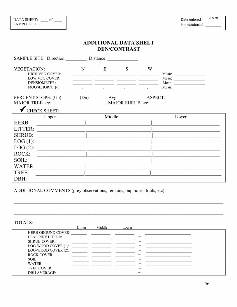
56

ADDITIONAL DATA SHEETDEN/CONTRAST

SAMPLE SITE: Direction _________ Distance _____________

VEGETATION: N E S WHIGH VEG COVER: __________ __________ __________ __________ Mean: _________________

LOW VEG COVER: __________ __________ __________ __________ Mean: ________________DENSIOMETER: __________ __________ __________ __________ Mean: ________________MOOSEHORN: (c)_____ _____,____ _____,_____ ____,_____ _____,_____ Mean: ________________

PERCENT SLOPE: (Up)________(Dn)________ Avg _______ ASPECT: ___________________MAJOR TREE SPP: ____________________________ MAJOR SHRUB SPP: _____________________________________

CHECK SHEET: Upper Middle Lower

HERB: __________________|________________________|_________________________LITTER: __________________|________________________|_________________________SHRUB: __________________|________________________|_________________________LOG (1): __________________|________________________|_________________________LOG (2): __________________|________________________|_________________________ROCK: __________________|________________________|_________________________SOIL: __________________|________________________|_________________________WATER: __________________|________________________|__________________________TREE: __________________|________________________|__________________________DBH: | |

ADDITIONAL COMMENTS (prey observations, remains, pup holes, trails, etc):________________________

__________________________________________________________________________________________

__________________________________________________________________________________________

TOTALS: Upper Middle Lower

HERB GROUND COVER: ________ __________ __________ = ________________________LEAF/PINE LITTER: ________ __________ __________ = ________________________SHRUB COVER: ________ __________ __________ = ________________________LOG-WOOD COVER (1): ________ __________ __________ = ________________________LOG-WOOD COVER (2): ________ __________ __________ = ________________________ROCK COVER: ________ __________ __________ = ________________________SOIL: ________ __________ __________ = ________________________WATER: ________ __________ __________ = ________________________TREE COVER: ________ __________ __________ = ________________________DBH AVERAGE: ________ __________ __________ = ________________________

Data entered(initials)

into database: _________

DATA SHEET: ____ of ____SAMPLE SITE: ____________

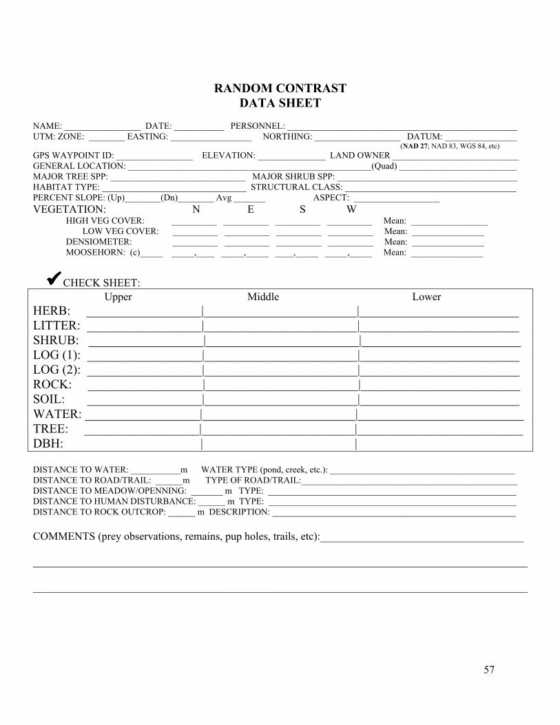
57

RANDOM CONTRASTDATA SHEET

NAME: _________________ DATE: ___________ PERSONNEL: ___________________________________________________UTM: ZONE: ________ EASTING: __________________ NORTHING: ___________________ DATUM: ________________

(NAD 27; NAD 83, WGS 84, etc)GPS WAYPOINT ID: _________________ ELEVATION: _______________ LAND OWNER ____________________________GENERAL LOCATION: ______________________________________________________(Quad) __________________________MAJOR TREE SPP: ______________________________ MAJOR SHRUB SPP: ________________________________________HABITAT TYPE: ________________________________ STRUCTURAL CLASS: ______________________________________PERCENT SLOPE: (Up)________(Dn)________ Avg _______ ASPECT: ___________________VEGETATION: N E S W

HIGH VEG COVER: __________ __________ __________ __________ Mean: _________________LOW VEG COVER: __________ __________ __________ __________ Mean: ________________

DENSIOMETER: __________ __________ __________ __________ Mean: ________________MOOSEHORN: (c)_____ _____,____ _____,_____ ____,_____ _____,_____ Mean: ________________

CHECK SHEET: Upper Middle Lower

HERB: __________________|________________________|_________________________LITTER: __________________|________________________|_________________________SHRUB: __________________|________________________|_________________________LOG (1): __________________|________________________|_________________________LOG (2): __________________|________________________|_________________________ROCK: __________________|________________________|_________________________SOIL: __________________|________________________|_________________________WATER: __________________|________________________|__________________________TREE: __________________|________________________|__________________________DBH: | |

DISTANCE TO WATER: ___________m WATER TYPE (pond, creek, etc.): _________________________________________DISTANCE TO ROAD/TRAIL: ______m TYPE OF ROAD/TRAIL:________________________________________________DISTANCE TO MEADOW/OPENNING: _______ m TYPE: _______________________________________________________DISTANCE TO HUMAN DISTURBANCE: ______ m TYPE: _______________________________________________________DISTANCE TO ROCK OUTCROP: ______ m DESCRIPTION: ______________________________________________________

COMMENTS (prey observations, remains, pup holes, trails, etc):_____________________________________

__________________________________________________________________________________________

__________________________________________________________________________________________

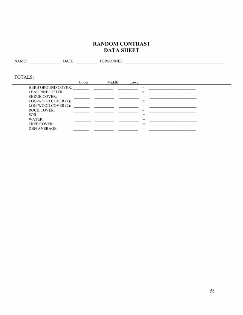
58

RANDOM CONTRASTDATA SHEET

NAME: _________________ DATE: ___________ PERSONNEL: ___________________________________________________

TOTALS: Upper Middle Lower

HERB GROUND COVER: ________ __________ __________ = ________________________LEAF/PINE LITTER: ________ __________ __________ = ________________________SHRUB COVER: ________ __________ __________ = ________________________LOG-WOOD COVER (1): ________ __________ __________ = ________________________LOG-WOOD COVER (2): ________ __________ __________ = ________________________ROCK COVER: ________ __________ __________ = ________________________SOIL: ________ __________ __________ = ________________________WATER: ________ __________ __________ = ________________________TREE COVER: ________ __________ __________ = ________________________DBH AVERAGE: ________ __________ __________ = ________________________

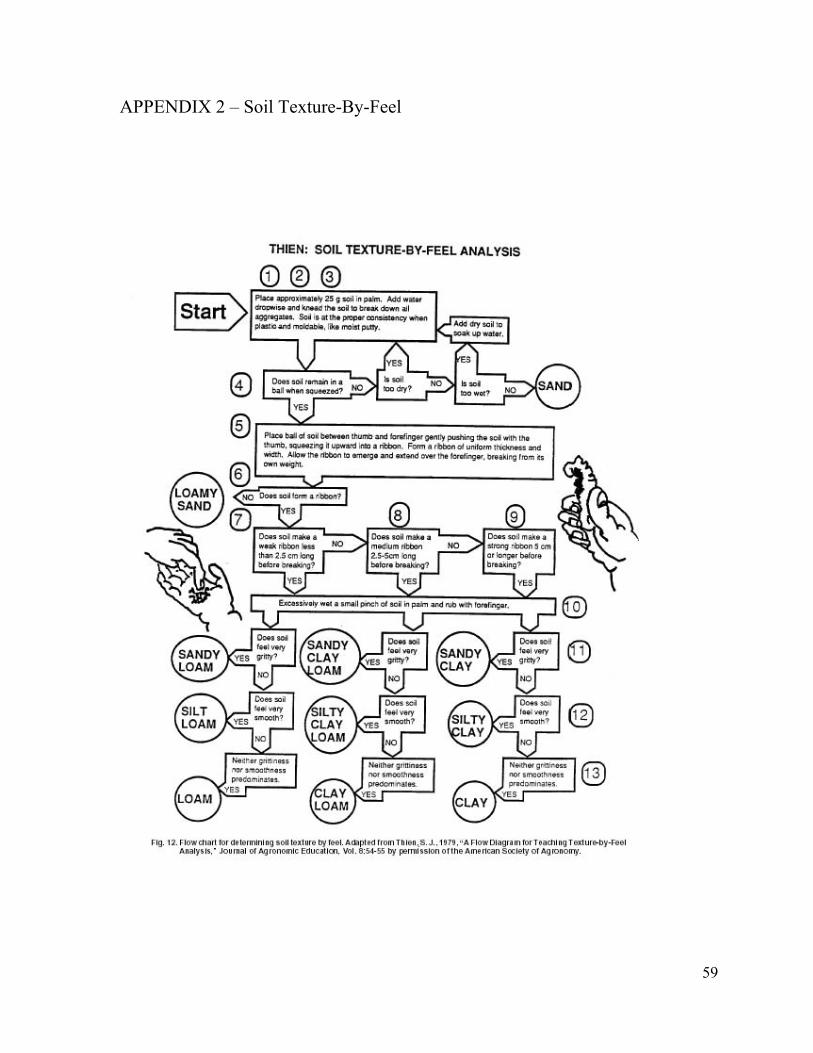
59

APPENDIX 2 – Soil Texture-By-Feel

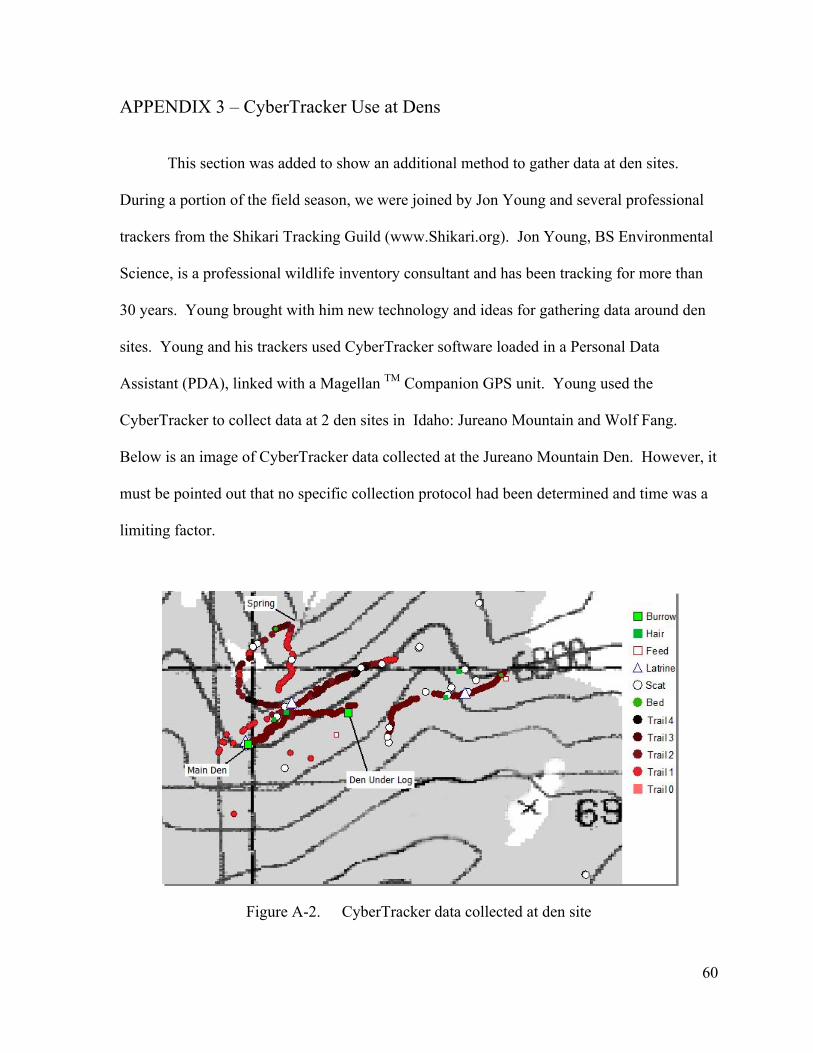
60

APPENDIX 3 – CyberTracker Use at Dens

This section was added to show an additional method to gather data at den sites.

During a portion of the field season, we were joined by Jon Young and several professional

trackers from the Shikari Tracking Guild (www.Shikari.org). Jon Young, BS Environmental

Science, is a professional wildlife inventory consultant and has been tracking for more than

30 years. Young brought with him new technology and ideas for gathering data around den

sites. Young and his trackers used CyberTracker software loaded in a Personal Data

Assistant (PDA), linked with a Magellan TM Companion GPS unit. Young used the

CyberTracker to collect data at 2 den sites in Idaho: Jureano Mountain and Wolf Fang.

Below is an image of CyberTracker data collected at the Jureano Mountain Den. However, it

must be pointed out that no specific collection protocol had been determined and time was a

limiting factor.

Figure A-2. CyberTracker data collected at den site

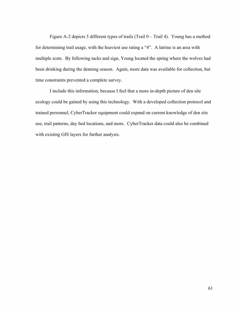
61

Figure A-2 depicts 5 different types of trails (Trail 0 – Trail 4). Young has a method

for determining trail usage, with the heaviest use rating a “4”. A latrine is an area with

multiple scats. By following tacks and sign, Young located the spring where the wolves had

been drinking during the denning season. Again, more data was available for collection, but

time constraints prevented a complete survey.

I include this information, because I feel that a more in-depth picture of den site

ecology could be gained by using this technology. With a developed collection protocol and

trained personnel, CyberTracker equipment could expand on current knowledge of den site

use, trail patterns, day bed locations, and more. CyberTracker data could also be combined

with existing GIS layers for further analysis.

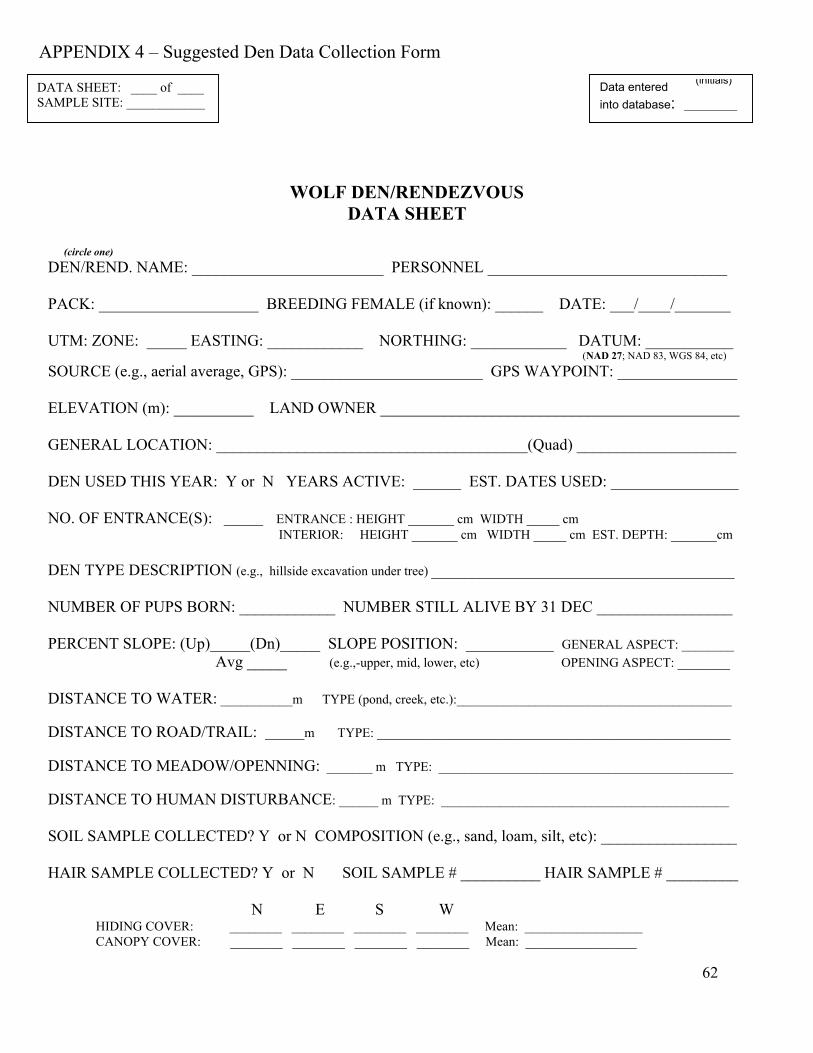
62

WOLF DEN/RENDEZVOUSDATA SHEET

(circle one)

DEN/REND. NAME: ________________________ PERSONNEL ______________________________

PACK: ____________________ BREEDING FEMALE (if known): ______ DATE: ___/____/_______

UTM: ZONE: _____ EASTING: ____________ NORTHING: ____________ DATUM: ___________ (NAD 27; NAD 83, WGS 84, etc)

SOURCE (e.g., aerial average, GPS): ________________________ GPS WAYPOINT: _______________

ELEVATION (m): __________ LAND OWNER _____________________________________________

GENERAL LOCATION: _______________________________________(Quad) ____________________

DEN USED THIS YEAR: Y or N YEARS ACTIVE: ______ EST. DATES USED: ________________

NO. OF ENTRANCE(S): ______ ENTRANCE : HEIGHT _______ cm WIDTH _____ cm INTERIOR: HEIGHT _______ cm WIDTH _____ cm EST. DEPTH: _______cm

DEN TYPE DESCRIPTION (e.g., hillside excavation under tree) ______________________________________

NUMBER OF PUPS BORN: ____________ NUMBER STILL ALIVE BY 31 DEC _________________

PERCENT SLOPE: (Up)_____(Dn)_____ SLOPE POSITION: ___________ GENERAL ASPECT: ________ Avg _____ (e.g.,-upper, mid, lower, etc) OPENING ASPECT: ________

DISTANCE TO WATER: ___________m TYPE (pond, creek, etc.):__________________________________________

DISTANCE TO ROAD/TRAIL: ______m TYPE: ______________________________________________________

DISTANCE TO MEADOW/OPENNING: _______ m TYPE: _____________________________________________

DISTANCE TO HUMAN DISTURBANCE: ______ m TYPE: ____________________________________________

SOIL SAMPLE COLLECTED? Y or N COMPOSITION (e.g., sand, loam, silt, etc): _________________

HAIR SAMPLE COLLECTED? Y or N SOIL SAMPLE # __________ HAIR SAMPLE # _________

N E S WHIDING COVER: ________ ________ ________ ________ Mean: __________________

CANOPY COVER: ________ ________ ________ ________ Mean: _________________

Data entered(initials)

into database: _________

DATA SHEET: ____ of ____SAMPLE SITE: ____________

APPENDIX 4 – Suggested Den Data Collection Form

63

HABITAT TYPE: ___________________________ STRUCTURAL CLASS: ______________________________________

MAJOR TREE SPP: _______________________________________________________________________________________

MAJOR SHRUB SPP: _____________________________________________________________________________________

PHOTOS TAKEN: Y or N EXPOSURE NUMBERS: _____ to ______ DIGITAL: Y or N

OBSERVATIONS (e.g., trails, day beds, bones, scats, ground cover):____________________________________________________________________________________________________________________________________________________________________________________________________________________________________________________________________________________________________________________________________________________________________________________________________________________________________________________________________________

DEN SITE SKETCH

Sketch interior shape (note measurements)