Please cite this paper as:

Balestra, C. and J. Sultan (2013), “Home Sweet Home: TheDeterminants of Residential Satisfaction and its Relation withWell-being”, OECD Statistics Working Papers, 2013/05,OECD Publishing, Paris.http://dx.doi.org/10.1787/5jzbcx0czc0x-en

OECD Statistics Working Papers2013/05

Home Sweet Home: TheDeterminants of ResidentialSatisfaction and its Relationwith Well-being

Carlotta Balestra, Joyce Sultan

Unclassified STD/DOC(2013)5 Organisation de Coopération et de Développement Économiques Organisation for Economic Co-operation and Development 23-Dec-2013 ___________________________________________________________________________________________

English - Or. English STATISTICS DIRECTORATE

HOME SWEET HOME: THE DETERMINANTS OF RESIDENTIAL SATISFACTION AND ITS RELATION WITH WELL-BEING WORKING PAPER No. 54.

This paper has been prepared by Carlotta Balestra, Policy Analyst in the OECD Statistics Directorate, and Joyce Sultan, who was a consultant in the OECD Statistics Directorate at the time of writing this report.

Contact: Carlotta Balestra (tel+33 1 45 24 94 36, email carlotta.balestra@oecd.org)

JT03350773

Complete document available on OLIS in its original format This document and any map included herein are without prejudice to the status of or sovereignty over any territory, to the delimitation of international frontiers and boundaries and to the name of any territory, city or area.

STD/D

OC

(2013)5 U

nclassified

English - O

r. English

STD/DOC(2013)5

2

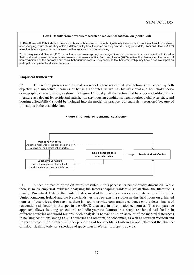
TABLE OF CONTENTS

HOME SWEET HOME: THE DETERMINANTS OF RESIDENTIAL SATISFACTION AND ITS RELATION WITH WELL-BEING ............................................................................................................... 4

OECD STATISTICS WORKING PAPER SERIES ...................................................................................... 5

ACKNOWLEDGMENTS .............................................................................................................................. 6

ABSTRACT .................................................................................................................................................... 7

RÉSUMÉ ........................................................................................................................................................ 7

Introduction ................................................................................................................................................. 8 From housing to neighbourhood: residential well-being ............................................................................. 8 Residential satisfaction .............................................................................................................................. 14 Empirical framework ................................................................................................................................. 17 Results ....................................................................................................................................................... 22 Conclusion ................................................................................................................................................. 28

REFERENCES ............................................................................................................................................. 36

ANNEX A: THE DETERMINANTS OF SATISFACTION WITH LOCAL ENVIRONMENTAL QUALITY ..................................................................................................................................................... 29

ANNEX B: THE DETERMINANTS OF SELF-REPORTED VICTIMISATION AND THE FEELING OF SECURITY ................................................................................................................................................... 31

Tables

Table 1. The scales of neighbourhood ................................................................................................ 11 Table 2. Differences in housing conditions ......................................................................................... 18 Table 3. Summary of explanatory variables available in EU-SILC .................................................... 20 Table 4. Summary of the explanatory variables available in the Gallup World Poll .......................... 21 Table 5. The determinants of housing satisfaction in EU-SILC ......................................................... 24 Table 6. The determinants of housing satisfaction in Gallup .............................................................. 27 Table A.1. The determinants of satisfaction with environmental quality ........................................... 30 Table B.1. The determinants of self-reported assault and the feeling of security ............................... 32

Figures

Figure 1. A model of residential satisfaction ........................................................................................ 17

STD/DOC(2013)5

3

Boxes

Box 1. The effects of housing conditions on people’s health ...................................................................... 9 Box 2. Defining the neighbourhood .......................................................................................................... 11 Box 3. Conceptualising and measuring housing affordability .................................................................. 13 Box 4. Results from previous research on residential satisfaction ............................................................ 16

STD/DOC(2013)5

4

HOME SWEET HOME: THE DETERMINANTS OF RESIDENTIAL SATISFACTION AND ITS RELATION WITH WELL-BEING

Carlotta Balestra and Joyce Sultan

STD/DOC(2013)5

5

OECD STATISTICS WORKING PAPER SERIES

The OECD Statistics Working Paper Series - managed by the OECD Statistics Directorate - is designed to make available in a timely fashion and to a wider readership selected studies prepared by OECD staff or by outside consultants working on OECD projects. The papers included are of a technical, methodological or statistical policy nature and relate to statistical work relevant to the Organisation. The Working Papers are generally available only in their original language - English or French - with a summary in the other.

Comments on the papers are welcome and should be communicated to the authors or to the OECD Statistics Directorate, 2 rue André Pascal, 75775 Paris Cedex 16, France.

The opinions expressed in these papers are the sole responsibility of the authors and do not necessarily reflect those of the OECD or of the governments of its Member countries.

http://www.oecd.org/std/research

STD/DOC(2013)5

6

ACKNOWLEDGMENTS

Earlier drafts of this paper have benefited from detailed comments and suggestions provided by Marco Mira d’Ercole, Anita Woelfl and Carrie Exton. The authors gratefully acknowledge Gallup Europe for the access to the micro-records from the Gallup World Poll. The analysis presented here has been carried out in the context of the preparation of the OECD report “How’s Life? Measuring well-being”. The usual disclaimer applies.

STD/DOC(2013)5

7

ABSTRACT

Housing is a core element of people’s material living standards. It is essential to meet basic needs, such as for shelter from weather conditions, and to offer a sense of personal security, privacy and personal space. Good housing conditions are also essential for people’s health and affect childhood development. Further, housing costs make up a large share of the household budget and constitute the main component of household wealth. Residential satisfaction is a broad concept, and is associated with multidimensional aspects including physical, social, and neighbourhood factors, as well as psychological and socio-demographic characteristics of the residents. By taking advantage of two household surveys (the EU-SILC ad hoc module on housing for European countries; and the Gallup World Poll for OECD countries and other major economies), this paper uses ordered probit analysis to explore the link between households’ residential satisfaction and a number of variables related to individuals, the households to which they belong, and the characteristics of the dwelling and neighbourhood where they live. The major findings of this analysis show a complex relationship between residential satisfaction and housing characteristics including neighbourhood’s features. Individual and household socio-demographic characteristics (e.g. age, gender, education) play a secondary role once dwelling and neighbourhood features are controlled for. Understanding the factors that lead to satisfaction with housing and residential environment is key for planning successful and effective housing policies.

Keywords: Housing satisfaction, Well-being, Household, Neighbourhood, Survey.

RÉSUMÉ

Le logement est un aspect essentiel des conditions de vie matérielles. Il doit à la fois répondre aux besoins fondamentaux, en offrant notamment un abri contre les intempéries, et donner aux individus un sentiment de sécurité et un espace d’intimité. Les conditions de logement jouent également un rôle capital dans la santé des individus et le développement des enfants. Par ailleurs, le coût du logement représente une part importante du budget des ménages et constitue leur principal patrimoine. La notion de satisfaction vis-à-vis du logement est un concept large, multidimensionnel, et incluant des facteurs physiques et sociaux ainsi que certaines caractéristiques psychologiques et sociodémographiques des résidents. Combinant deux enquêtes différentes sur les conditions de vie des ménages (le module EU-SILC sur le logement et l’enquête Gallup World Poll sur les pays de l’OCDE ainsi que sur les économies majeures), ce papier fait usage d’une analyse en probit ordonné afin d’explorer le lien entre la satisfaction des ménages vis-à-vis de leur logement et un ensemble de facteurs ayant attrait à la situation personnelle des individus ainsi que les caractéristiques de leur logement et de la zone de résidence. Cet article caractérise une relation complexe entre la satisfaction vis-à-vis du logement et ces caractéristiques ainsi que certains aspects du voisinage. Les caractéristiques sociodémographique du ménage (comme l’âge, le genre, le niveau d’éducation…) n’ont finalement qu’un rôle mineur dans l’explication de la satisfaction pour le logement. Une bonne compréhension des facteurs visant à un accroissement de la satisfaction vis-à-vis du logement est essentielle pour l’élaboration de politiques effectives sur le logement.

Mots clés: Satisfaction à l’égard du logement, Bien-être, Ménage, Zone de résidence, Enquête.

STD/DOC(2013)5

8

Introduction

1. Over the past few years, housing has been on the top of the political agenda. After having played an important role as a trigger of the crisis, the persistence of depressed conditions in the housing market risks today derailing prospects of a sustained a recovery of the global economy (OECD, 2011a). While housing is often perceived as a barometer for gauging the health or ill-health of a nation, it is also essential to people’s quality of life: not only because it represents the single largest item in households’ budgets and balance sheets (Bruning et al., 2004), but also because it greatly affects individual’s well-being through a range of economic, social and psychological channels.

2. Research conducted in various countries has provided evidence that having satisfactory accommodation is often at the top of people’s human needs (Kiel and Mieszkowski, 1990). Housing provides a shelter from extreme weather conditions and a place where to sleep and rest. But a house is also “the centre of family life, where children are born and raised, where socialisation takes place and family ties are nurtured” (Alber and Fahey 2004, p. 15). All these elements make a “house” a “home” and are intrinsically valuable to people.

3. Since housing is an important investment and a right of every individual, the ultimate goal of any housing programme should be to enhance people’s housing opportunities and to ensure equitable access to decent housing, in order to satisfy the needs of its occupants and increase their well-being. In order to design and implement any successful housing policy, it is fundamental to understand which factors and drivers determine people satisfaction with respect to their housing conditions.

4. The remainder of the paper is structured as follows. Section 2 spells out the impact of housing and neighbourhoods on people’s life. Section 3 reviews the literature on housing and residential satisfaction. Section 4 describes the empirical model as well as the data and the variables used in this paper, while Section 5 discusses the results of the model used to test the effects of housing and neighbourhood characteristics on residential satisfaction. Section 6 summarises and concludes.

From housing to neighbourhood: residential well-being

5. The appreciation that the place of living matters for people’s well-being is well acknowledged. Poor housing and neighbourhood conditions pose a threat to people’s quality of life, their physical and mental health and self-development. This section considers three important and inter-related aspects of residential housing, and their links to people’s well-being: the physical conditions within homes; the conditions in the neighbourhoods surrounding homes; and housing affordability, which shapes not only home and neighbourhood conditions but also the overall ability of individuals and families to make healthy choices.

Housing conditions and well-being

6. Housing conditions strongly influence people’s quality of life. First of all, adequate housing protects individuals and families from harmful exposures and provides them with a sense of privacy, security, stability, and control. Conversely, poor quality and inadequate housing (e.g. houses lacking access to basic sanitation and functional utilities, or characterised by overcrowding, etc.) contributes to health problems such as infectious and chronic diseases as well as injuries (see Box 1).

STD/DOC(2013)5

9

Box 1. The effects of housing conditions on people’s health

Recent research has provided evidence of sizeable and long-ranging effects of inadequate housing on people’s mental and physical health. For instance:

• Lead poisoning irreversibly affects the development of the brain and of the nervous system, resulting in lower IQ, reading disabilities and possibly leading to children’s low school performance (OECD, 2009). Most exposures occur in dwellings that contain lead-based paint and lead in the plumbing systems. Deteriorating paint in older homes is the primary source of lead exposure for children, who ingest paint chips and inhale lead-contaminated dust.

• Sub-standard housing conditions such as water leaks, poor ventilation, dirty carpets and pest infestation can lead to an increase in mould, mites and other allergens associated with poor health. Indoor allergens and damp housing conditions play an important role in the development and exacerbation of respiratory conditions including asthma. Approximately 40% of diagnosed asthma among U.S. children is believed to be attributable to residential exposures (Lanphear et al., 2001).

• Exposure to very high or very low indoor temperatures can be detrimental to health status. Cold indoor conditions have been associated with poorer health, including an increased risk of cardiovascular disease. Extreme low and high temperatures have been associated with higher mortality, especially among vulnerable populations such as the elderly (Shaw, 2004).

• Residential exposure to tobacco smoke, pollutants from heating and cooking with gas, volatile organic compounds and asbestos have been linked with respiratory illness and some types of cancer (Environmental Protection Agency, 2006; Landrigan et al., 1999; Weitzman et al. 1990). Poor ventilation may also increase exposure to harmful compounds.

• Injuries occurring at home represent a major cause of emergency-department visits and hospital admissions. Contributing factors include structural features of the home such as steep staircases and balconies; lack of safety devices such as window guards and smoke detectors; and sub-standard heating systems (Shaw, 2004).

• Overcrowding has been linked to both physical illness, including infectious diseases such as tuberculosis and respiratory infections (Krieger and Higgins, 2002), and to psychological distress among both adults and children. Children who live in crowded housing may have poorer cognitive and psychomotor development (OECD, 2009) or be more anxious, socially withdrawn, stressed or aggressive (Evans, 2006). Homelessness and living in temporary housing have also been related to behavioural problems among children (Zima et al., 1994).

• Preliminary research suggests that residents’ perceptions of their homes (e.g. satisfaction with their dwelling or concerns about indoor air quality) are associated with low self-rated health status (Dunn and Hayes, 2000).

Poor indoor air quality, lead paint, lack of home safety devices, and other housing hazards often cluster in the same homes, exposing families and especially children to greater risk of multiple health problems. As families with fewer financial resources are most likely to experience unhealthy and unsafe housing conditions, and to be the least able to remedy them, sub-standard housing contributes to spreading disparities in health conditions across socio-economic groups. Therefore, health problems originated in poor housing conditions can be considered as indicative of social inequalities (Dunn, 2000).

Source: Adapted from Mueller and Tighe, 2007.

STD/DOC(2013)5

10

7. Lack of appropriate accommodation may also threaten the functioning of a family. Crowded accommodation, in particular, is a potentially destructive force: it can lead to tensions among family members and even family breakdown and it is generally harmful to the development of community ties. Sub-standard housing conditions may also lead to social isolation because occupants are reluctant to invite guests into their homes. High-rise buildings may also inhibit social interaction because they lack common spaces (Giloran, 1968).

Neighbourhood conditions and well-being

8. Along with conditions in the home, conditions in the neighbourhoods where homes are located have been shown to affect people’s well-being and health quality. Neighbourhoods can be defined as the localities in which people live, and are an appropriate scale for analysis of how local conditions affect people’s life (for a more detailed definition of the concept of neighbourhood see Box 2). Neighbourhoods can affect people’s quality of life in several ways. First, through their physical characteristics: people’s well-being can be adversely affected by poor air and water quality or by proximity to facilities that produce hazardous substances. A neighbourhood’s physical characteristics may promote (or hamper) good health conditions by providing places for children to play and for adults to exercise that are free from litter, crime, violence and pollution. For instance, research has shown how a sub-standard built environment (i.e., the characteristics of the buildings, streets and other constructed features of the neighbourhoods) can be associated with a higher incidence of obesity, cardiovascular diseases, depression and smoking habits (Chuang et al., 2005; Diez Roux et al., 2001; Morland et al., 2006; Schulz et al., 2000).

9. Second, people’s well-being can also be shaped by the social environment of the neighbourhood, i.e. by the characteristics of the social relationships among its residents, including the degree of mutual trust and the feelings of connectedness among neighbours. Residents of “close-knit” neighbourhoods are more likely to work together to achieve common goals (e.g., cleaner and safer public spaces), to exchange information (e.g., regarding childcare or jobs), and to maintain informal social controls (e.g., discouraging crime or other undesirable behaviours such as drunkenness, littering and graffiti), all of which can directly or indirectly benefit well-being (Putman, 1993). Children in more closely-knit neighbourhoods are more likely to receive guidance from several adults and less likely to engage in health-damaging behaviours like smoking, drinking, drug use or gang involvement (Aneshensel and Sucoff, 1996). Neighbourhoods in which residents express mutual trust have also lower homicide rates (Morenoff et al., 2001).

10. The availability of services and opportunities in neighbourhoods is another pathway through which neighbourhoods can influence people’s well-being. Access to employment opportunities and public services – including efficient transportation, an effective police force, and good schools – directly affects people’s well-being.

11. However, not all neighbourhoods enjoy these opportunities and resources, and access to neighbourhoods with healthy conditions may depend on a household’s economic and social resources. Housing discrimination often limits the ability of many low-income and minority families to move to healthy neighbourhoods.

STD/DOC(2013)5

11

Box 2. Defining the neighbourhood

‘Neighbourhood’ is a vague, loosely defined concept. Scholars investigating the impact of neighbourhood on people’s behaviour and well-being often do not provide an explicit definition of the term. In the literature, the neighbourhood may be seen as a source of place-identity, an element of urban form, or a unit of decision making. This co-dependence between the spatial and social aspects of neighbourhood is arguably one of the main reasons why the concept is difficult to define at both the conceptual and the operational level. Moreover, research often uses multiple definitions of a neighbourhood simultaneously, to reflect the fact that neighbourhood is not a static concept but rather a dynamic one (Talen and Shah, 2007).

In his seminal work Park (1916) laid the foundation for urban sociology by defining a neighbourhood as a subsection of a larger community (or city), a collection of both people and institutions occupying a spatially defined area influenced by ecological, cultural, and sometimes political forces. Followers of this line of thought tend to consider neighbourhoods as discrete, non-overlapping communities, leading to the common use of census tracts or administratively-defined areas for analysing neighbourhood effects. Suttles (1972) argued that the local community is best thought of not as a single, segregated entity, but rather as a hierarchy of ecological units nested within successively larger communities. According to Suttles (1972), the neighbourhood exists at three different scales, which have different functions and whose effects operate through different mechanisms (Table 1).

Table 1. The scales of neighbourhood

Source: Suttles (1972).

Galster (2001) defined a neighbourhood as a ‘complex commodity’ that is produced and consumed by four different actors: households, businesses, property owners and local government. Households consume neighbourhood services through the act of occupying a residential unit and using the surrounding private and public spaces, thereby gaining some degree of satisfaction from the quality of their residential life. Businesses consume neighbourhood services through the act of occupying a non-residential structure (store, office, factory), thereby gaining a certain flow of net revenues or profits associated with that venue. Property owners consume neighbourhood services by extracting rents and/or capital gains from the land and buildings owned in that location. Finally, local governments rely on neighbourhood by extracting tax revenues, typically from owners, based on the assessed values of residential and non-residential properties.

While there is little agreement on the concept of neighbourhood, most researchers would agree that “neighbourhood is a function of the inter-relationships between people and the physical and social environments” (Knox and Pinch, 2000, p. 8). Brower (1996), for instance, explained that its form is derived from a particular pattern of activities, the presence of a common visual motif, an area with continuous boundaries or a network of often travelled streets.

Wilkenson (1989, p. 339) argued that “community is not a place, but it is a place-orientated process. It is not the sum of social relationships in a population but it contributes to the wholeness of local social life. A community is a process of interrelated actions through which residents express their shared interest in the local society”. Glass (1948, p. 18) similarly defined the neighbourhood as a “distinct territorial group, distinct by virtue of the specific physical characteristics of the area and the specific social characteristics of the inhabitants”.

Scale Predominant function MechanismPsycho-social benefits Familiarity

(i.e. identity, belonging) Community

Residential activities PlanningSocial status and position Social provision

Housing marketLansdcape of social and Employment connectionseconomic opportunities Leisure activities

Social networks

Home area

Locality

Urban district

STD/DOC(2013)5

12

Box 3. Defining the neighbourhood (continued)

Recently, urban sociology has also focused on people’s perception of neighbourhood. Motivated by the uncertainty about how to construct operational units for neighbourhoods, in view of the many factors influencing residents’ perception, Coulton et al. (2001) examined residents’ perception through ‘mental maps’. In their research, Coulton et al. asked 140 parents of minor children living in seven census-defined block groups in Cleveland to draw a map of what they consider as the boundaries of their neighbourhoods. The study identified large discrepancies between resident-defined neighbourhoods and census geography; this suggests that individuals residing in close proximity can differ markedly from one another in how they define the physical space of their neighbourhood depending on their race, age and gender.

Grannis (2003) also attempted to construct practical representations of neighbourhoods. Grannis modelled cities as multiple independent ‘islands’ consisting of discontinuous networks of pedestrian streets that are separated by major thoroughfares. By comparing these islands with residents’ cognitive maps of their neighbourhood, he showed that, while islands circumscribe residents’ perception of their neighbourhoods, residents typically perceive only a portion of their island as their neighbourhood.

Source: Adapted from Sampson et al. (2002) and Guo and Bhat (2007).

Housing affordability and well-being

12. Beyond its physical attributes, housing affects people’s well-being on account of its costs and affordability. There are many ways to define affordable housing.1 One possible way of making this concept operational, which is used by analysts in several OECD countries, is for a household to pay no more than 30 percent of its annual income on housing (Box 3). The lack of affordable housing represents a significant hardship for many low-income households and has clear implications for people’s well-being.2

13. The shortage of affordable housing limits households’ choices about where to live, often relegating lower-income families to sub-standard housing in unsafe neighbourhoods with higher rates of crime and poverty (Stegman, 1998) and fewer services and opportunities (e.g., parks, good schools, health-care centres, employment opportunities). Housing costs, when too high, can thus threaten households’ material well-being and economic security.

14. Moreover, when rents and housing loans or costs are unaffordable, it is difficult to cover other necessities such as food, thereby contributing directly to food insecurity. When families spend a too high percentage of their income to obtain adequate housing, the financial resources that can be spent on food, access to health care services and other determinants of health is significantly reduced (Burke and Ralston, 2003). This in turn places some households at risk of not being able to sustain their tenancy or home ownership, creating an increased potential for eviction and homelessness (Crowley, 2003). Unstable or unaffordable housing situations may force low-income families to move frequently to find affordable housing. Frequent moves in young childhood or adolescence can impair youth’s educational attainments as well as psychological and emotional development (Hartman and Franke, 2003; Mueller and Tighe, 2007; Rumberger, 2003).

STD/DOC(2013)5

13

Box 3. Conceptualising and measuring housing affordability

One of the major issues raised in the literature on housing is the ambiguity of the concept of affordability, and the way in which it is measured for specific policy purposes. Part of the difficulty in conceptualising housing affordability comes from the fact that it “jumbles together in a single term a number of disparate issues: the distribution of housing prices, the distribution of housing quality, the distribution of income, the ability of households to borrow, public policies affecting housing markets, conditions affecting the supply of new or refurbished housing, and the choices that people make about how much housing to consume relative to other goods. This mixture of issues raises difficulties in interpreting even basic facts about housing affordability.” (Quigley and Raphael, 2004, pp. 191-192).

To some extent, ambiguity in the conceptualisation of housing affordability is linked to different understandings of its causes and drivers (in particular, the degree to which the issue stems from inadequate household incomes or inadequate housing), to the nature of the housing system within nations, to inherited policy settings and the orientation of policy reforms. Despite the contested nature of the concept of housing affordability, working definitions and measures have been employed in various contexts. At large, housing affordability is a tenure-neutral term that denotes the relationship between household income and household expenditure relating to housing.

The Australian Bureau of Statistics measures ‘housing hardship’ by applying the “30/40 rule”. In this approach, housing affordability is compromised when households in the bottom 40 per cent of income distribution spend more than 30 per cent of their household income (adjusted for household size) on housing. Those who do not have affordable housing according to this criterion are said to be experiencing “housing stress”Error! Reference source not found., which may be measured in terms of people’s subjective experiences of managing housing costs (Yates and Milligan, 2007). Housing costs in Australia exclude electricity and other heating costs.

In the United States, housing affordability targets have been a key component of housing policy since the 1970s. Here, the conventional public policy indicator of affordability is the percentage of income spent on housing (Bogdon and Can, 1997). Typically, households that spend more than 30 per cent (raised from 25 per cent in 1981) of their income on housing are defined as being in “housing stress”, although the level at which this benchmark has been set has changed over time. Critics suggest that this type of indicator suffers from the fact that, for those on low incomes, an acceptable ratio (where, for example, one-third of income is spent on housing) may obscure the fact that the residual income is well below acceptable poverty thresholds. At the opposite, wealthy households (typically high – and to a lesser extent – middle income households) can decide to spend more than 30 per cent of their income without suffering from any material deprivation in terms of their everyday consumption. As for the affordability of owner-occupied housing, the Department of Housing and Urban Development (HUD) assumes that households should not spend more than 28 percent of their annual income to pay costs on the median-priced house. Costs include principal and interest payments, real estate taxes and homeowners’ insurance premiums.

STD/DOC(2013)5

14

Box 3. Conceptualising and measuring housing affordability (continued)

In contrast to the United States, housing affordability in the United Kingdom has been conceptualised more broadly to include housing supply, housing needs and housing costs. This broader approach reflects the considerable criticism of measures that focus only on the housing costs incurred by households, to the exclusion of other factors such as the ability of households to borrow and to the interaction of planning and social policies (Freeman et al., 2000). Accordingly, the UK Government’s Housing Green Paper (2007) does not provide a single definition of housing affordability but rather provides a framework for developing locally-determined targets. The Green Paper recommends that local authorities undertake assessments of affordable housing by taking into account prices and rents on the local house market, local incomes, the supply and suitability of existing affordable housing (including both subsidised and low cost market housing), the size and type of households, and the types of housing best suited to meet these local needs.

In Canada, policy makers have advocated a combined approach to housing affordability by applying a “norm rent income” value, which is used as the low-income cut-off. A household is said to be in housing need due to affordability problems if it spends more than 30% of its income on housing and its income falls below the ‘norm rent income’ required to rent an average dwelling suitable (in terms of number of bedrooms) and adequate for that household’s purpose. In this approach, “housing need” is assessed in relation to the three standards of adequacy, suitability and affordability. First, a household’s dwelling situation is evaluated against each of the standards. Then, if the household is found to have fallen below at least one of the standards, a means test is applied to determine whether or not the household in question could find an acceptable alternative for less than 30% of its before-tax income. If not, the household is said to have fallen into “core housing need”.

In some countries, an affordability limit is not set explicitly, but it is implicit in the policy that the government develops for its targeted housing allowance. Hills et al. (1990) noted that the idea behind the German model of the housing allowance is that rent for adequate housing should not exceed 25% of total household expenditures; though it may be as much as 30% for single-member households”.

In summary, there is growing recognition across OECD countries of the need for a broad and more encompassing understanding of housing affordability, which goes beyond the calculation of housing costs to income ratios. An analysis of housing expenditures and affordability, based only on household expenditures-to-income ratios, does not sufficiently take into account the quality of housing, the size of the housing inhabited, the protection of tenant rights, and other costs connected with housing (e.g. the costs of commuting). However, costs to income ratios continue to be viewed as an appropriate first step in calculating the cost component of housing affordability, with efforts underway to make such measures more sensitive to quality of housing, household composition and spatial variation.

1. Housing stress is a generic term used to denote the negative impact on households striving to secure adequate housing (for a review of the literature on the subject, see Gabriel et al., 2005).

Source: Adapted from Gabriel, M, et al. (2005),

Residential satisfaction

15. Mesch and Manor (1998) defined satisfaction as the evaluation by respondents of features of the physical and social environment. However, there is no consensus about the type of appraisal provided by respondents when questioned about their residential satisfaction. Some authors follow a purposive approach, where residents’ own goals are at the centre of the evaluation of residential satisfaction (Oseland, 1990). Canter and Rees (1982) define residential satisfaction as “a reflection of the degree to which the inhabitants feel their housing is helping them reach their goals”. This approach, rooted in a cognitive view, enables researchers to understand the extent to which different facets of housing and neighbourhood contribute to users’ satisfaction.

16. Other authors stressed that people are not only goal oriented, but also have affective relations with their surrounding environment. Moreover, evaluations of the environment usually involve

STD/DOC(2013)5

15

comparisons between what users have and what they would like to have. This is the premise of a second approach to residential satisfaction, called actual-aspirational gap approach (Galster, 1987).

17. Francescato et al. (1989) developed a more comprehensive approach to residential satisfaction. They noted that “the construct of residential satisfaction can be conceived as a complex, multidimensional, global appraisal combining cognitive, affective, and cognitive facets, thus fulfilling the criteria for defining it as an ‘attitude’”.

18. To complicate matters, it is important to recognise that a dwelling and its neighbourhood are more than just physical units. Most people chose to live in a house after careful considerations of many factors, some of which go beyond the physical and structural characteristics of the dwelling and of the surrounding area (e.g. local employment opportunities, efficiency of public transport, access to recreational areas, social networks). Onibokun (1974) notes that a dwelling that is adequate from the physical and design point of view may not necessarily be satisfactory from the household’s point of view. The concept of satisfactory housing conditions is therefore related not only to the physical, architectural and engineering components of the house, but also to the components of the surrounding environment. People’s residential satisfaction will also be influenced by the social, behavioural, cultural and demographic characteristics of the household.

19. The above considerations underscore the importance of combining objective indicators related to housing and the neighbourhood where people live with households’ subjective evaluations of residential attributes. Objective measures refer to the presence or lack of attributes, while subjective measures refer to the perceptions, feelings and attitudes towards the attributes of housing and neighbourhood.

20. Recent research in this field (Paris and Kangari, 2005; Mccrea, et al., 2005) has followed this integrating perspective and examined how residential satisfaction varies at different levels of analysis (e.g. dwelling, neighbourhood, metropolitan area and region). Although the way in which these levels are defined in these studies has depended on the context of the research and the interest of the researcher, the most common levels considered have been the housing unit and the neighbourhood (Amole, 2009), even though only few authors define neighbourhood precisely (Amerigo and Aragones, 1997).

21. In the last few decades, a growing body of literature has explored the determinants of satisfaction with the housing environment for a variety of population groups. The main findings of previous research on this topic are highlighted in Box 4.

STD/DOC(2013)5

16

Box 4. Results from previous research on residential satisfaction

Early empirical work on residential satisfaction used bivariate techniques to identify the correlates of residential satisfaction within particular demographic groups (e.g. the poor, the elderly, the disabled) or in particular types of cities. More recently, researchers have used multivariate techniques to test models of residential satisfaction with three sets of variables: i) individual and household socio-demographic characteristics, ii) objective characteristics and subjective perceptions of the dwelling, iii) objective features of, and subjective attitudes towards, the neighbourhood. Various characteristics of the residents as well as housing- and neighbourhood- related factors have been found to affect residential satisfaction in a complex way. For instance:

• Individuals who are less than 35 years of age are more likely to be dissatisfied with their dwelling than respondents who are aged 35 years or older (Van Praag et al., 2003). People aged 65 and over are usually the most satisfied with residential conditions, this being explained by their higher economic resources, smaller family size (Vera-Toscano and Ateca-Amestoy, 2008) and higher rates of home ownership among the elderly (Andrews and Caldera Sánchez, 2011).

• Similarly, women and married householders are more likely to be satisfied with housing conditions (Galster, 1987; Varady et al., 2001). Gender effects may be partly explained by a division of roles in the household, since housing activities are mostly allocated to women (Vera-Toscano and Ateca-Amestoy, 2008).

• Evidence is more inconsistent and conflicting for several socio-economic variables (income, education, employment, welfare). For example, one might assume that those with higher income have greater capacity to find a better home and neighbourhood, in which case income (and possibly education and employment) would be positively correlated with residential satisfaction (Freeman, 1998). On the other hand, however, high-income householders might have higher standards and aspirations, which might lead them to be more dissatisfied (Varady et al., 2001).

• Home owners are normally more satisfied with their homes and their neighbours than renters (Rohe and Basolo, 1997; Elsinga and Hoekstra, 2005; Shlay, 2006; Diaz-Serrano, 2009).0 Several authors have stated that home ownership also increases social capital, since home owners are more likely to invest in relationship with their neighbours, and to be concerned about the local amenities publicly provided (e.g., schooling or health care services).2 However, home ownership also limits mobility, which may impose costs in terms, for instance, of increased unemployment (Oswald, 1999; Parker et al., 2011). Moreover, for many households the mere fact of home ownership does not remove other housing burdens, such as high costs or inadequate quality.

• According to Diaz-Serrano (2005) individuals living in detached or semi-detached properties – rather than multiple occupancy dwellings (i.e. apartments, flats and bedsits) – tend to report higher levels of housing satisfaction in all European countries. With regard to accommodation type, Lane and Kinsey (1980) found that people living in different types of dwellings have different preferences for housing characteristics – possible reflecting differences in age, household composition, etc. – but that residents of single-family dwellings and duplexes had the highest levels of reported housing satisfaction compared to those living in other types of housing (i.e. multiple-occupancy dwellings).

• The structural features of the dwelling are also very influential. Diaz-Serrano (2006) observed that dwelling deficiencies – shortage of space, rot, leaky roofs, inadequate heating and insufficient light – exert a negative effect on housing satisfaction in all European countries. Research in the U.S. has confirmed such a relationship between actual features and physical amenities of the dwelling and the satisfaction of households (James, 2007). Length of residence is an important driver of residential satisfaction. The longer an individual lives in an area, the stronger their ties to that area tend to be and the higher the probability that they are residentially satisfied (Lu, 1999). At the neighbourhood-level, previous research identified a number of factors that are likely to lead to residential dissatisfaction, such as crime, noise, the presence of abandoned buildings or the lack of shared and natural spaces. Relatively few studies explicitly investigated the impact on residential satisfaction of other neighbourhood features such as location (e.g. distance from workplace and shopping sites) and availability and quality of public services (e.g. schools, childcare programs, medical care facilities, Grzeskowiak et al., 2003).

STD/DOC(2013)5

17

Box 4. Results from previous research on residential satisfaction (continued)

1. Diaz-Serrano (2009) finds that renters who become homeowners not only significantly increase their housing satisfaction, but also, after changing tenure status, they obtain a different utility from the same housing context. Using panel data, Clark and Oswald (2002) show that becoming a renter is associated with a significant drop in well-being.

2. Di Pasquale and Glaeser (1998) show that homeownership may encourage citizenship, as owners have an incentive to invest in their local environment because homeownership restrains mobility. Dietz and Haurin (2003) review the literature on the impact of homeownership on the economic and social behaviour of owners. They conclude that homeownership may have a positive impact on participation in political and social activities.

Empirical framework

22. This section presents and estimates a model where residential satisfaction is influenced by both objective and subjective measures of housing attributes, as well as by individual and household socio-demographic characteristics, as shown in Figure 1.3 Ideally, all the factors that have been identified in the literature as relevant for residential satisfaction (i.e. housing conditions, neighbourhood characteristics, and housing affordability) should be included into the model; in practice, our analysis is restricted because of limitations in the available data.

Figure 1. A model of residential satisfaction

23. A specific feature of the estimates presented in this paper is its multi-country dimension. While there is much empirical evidence analysing the factors shaping residential satisfaction, the literature is mainly US-centred. Outside the United States, most of the existing studies concentrate on localities in the United Kingdom, Ireland and the Netherlands. As the few existing studies in this field focus on a limited number of countries and/or regions, there is need to provide comparative evidence on the determinants of residential satisfaction in Europe, in the OECD area and in other major economies. This comparative approach allows focusing on cultural and idiosyncratic features that shape residential satisfaction in different countries and world regions. Such analysis is relevant also on account of the marked differences in housing conditions among OECD countries and other major economies, as well as between Western and Eastern Europe.4 For instance, a higher proportion of households in Eastern Europe self-report the absence of indoor flushing toilet or a shortage of space than in Western Europe (Table 2).

Subjective appraisal of structural, environmental and social attributes

Socio-demographic characteristics

Residential satisfaction

Objective variablesObjective measures of the presence or lack

of physical and structural attributes

Subjective variables

STD/DOC(2013)5

18

Table 2. Differences in housing conditions

Housing attributes Western Europe Eastern Europe Indoor flushing toilet 99.1% 93.1% Bath or shower 99.4% 93.6% Structural damages 15.3% 27.4% Adequate plumbing installations 92.1% 92.9% Adequate electrical installations 92.1% 95.3% Adequate heating installations 92.9% 99.7% Shortage of space 12.5% 21.2% Number of rooms per person 1.8 1.1

Note. The data show the share of respondents self-reporting the presence in the dwelling of: indoor flushing toilet; bath or shower; structural damages; adequate plumbing, electrical and heating installations; and lack of space, respectively. The variable “number of rooms per person” has been obtained by dividing the total number of rooms available to the household by the household size.

Source: OECD calculations based on EU-SILC 2007.

Sampling and sample characteristics

24. To analyse the relationship between objective measures of residential conditions, subjective appraisal and background variables, this study relies on data from two different surveys. In each survey, the same questionnaire was used in all countries included in the sample; this provides a good opportunity to make cross-country comparisons while, at the same time, ensuring enough data to permit within-country disaggregation, for example, by age, gender, income or education.

25. The first survey is the EU Statistics on Income and Living Conditions (EU-SILC). An ad hoc module on housing conditions was fielded in 2007, covering the 27 EU countries plus Iceland and Norway. The main advantage of the EU-SILC ad hoc module is that it is rich in measures on housing and neighbourhoods; these range from intrinsic features of the home to households’ perception of safety and environmental quality in the surrounding area. The sample is made up of 440,400 individuals over 16 years old nested in 207,000 household units. From these data, a sample was drawn of 174,186 respondents who provided complete information on the variables considered in the model. The final sample was split and separate analyses performed for Western-European and Eastern-European countries, so as to take into account differences in both objective housing conditions and in cultural backgrounds that characterise European citizens.

26. The second source of information is the Gallup World Poll, which includes several questions on residential satisfaction. Although being less detailed than the EU-SILC ad hoc module, this survey has the advantage of covering all the OECD countries and other major economies over the period 2005-2007.5 The sample comprises more than 117,000 individuals aged 15 and over. From these data, a sample of 15,713 questionnaire respondents for which complete information is available has been selected. The final sample was split and separate analyses performed for OECD countries and other major economies, in order to better take into account both different housing conditions and particular cultural values and preferences that make people attach different levels of importance to various attributes of housing and neighbourhood.

Dependent variable

27. For both data sets, the dependent variable is a measure of housing satisfaction. In the EU-SILC ad hoc module, respondents are asked to rate their satisfaction with the dwelling where they live on a Likert-type scale ranging from 0 (very dissatisfied) to 3 (very satisfied). As in Eastern Europe very few

STD/DOC(2013)5

19

people declare to be very satisfied with their housing conditions, this variable was re-coded into three categories: very dissatisfied (0), dissatisfied (1) and satisfied or very satisfied (2 and 3). The question related to housing satisfaction available in the Gallup World Poll reads as follows: “Are you satisfied or dissatisfied with your current housing, dwelling, or place you live?”, with answers taking the form of either “no” (0) or “yes” (1).6

Independent variables

28. The selection of independent variables for this study was guided by past research on housing satisfaction (see Box 4), the purpose of this research and data availability. Three groups of independent variables are considered.

• The first group includes variables representing individual and household attributes, such as age, gender, education attainment, income and self-reported health status. Household type (e.g. single-headed household, presence of children) is also considered to control for possible differences in the assessment of same housing conditions by respondents with different household background. Households are classified based on the presence or absence of spouse and children.7

• The second group of independent variables relates to basic characteristics and conditions of the home environment that may have direct adverse effects on people’s health and well-being. This set includes the following variables: presence of bath or shower in the dwelling; presence of indoor flushing toilets; presence of structural damages; adequate electrical installations; adequate plumbing installations; dwelling equipped with heating facilities; and house comfortably warm during winter time. A variable for “number of rooms for person” was also added as a proxy for overcrowding.8 As this metric does not take into account the dwelling overall size (e.g. the number of square meters per person), the information on housing overcrowding has been complemented by a variable on subjective perceptions of available space (“shortage of space”), which gives an idea of people’s perception of space and feeling of being cramped. Tenure and housing costs as a percentage of income were also considered.9

• The third set includes variables related to individuals’ perceptions of their neighbourhoods. These variables control for the presence of neighbourhood characteristics which are perceived as bothersome by respondents, such as the level of crime or noise. Equally, dummies to indicate the presence of certain amenities (e.g. health care services, primary school, access to roads and public transports) were included as a proxy for neighbourhood quality. Moreover, since the dwelling’s location also matters for well-being (e.g. due to differential exposure to specific hazards or the proximity of public services) a locational variable distinguishing between individuals residing in rural, semi-rural and urban settings was considered.

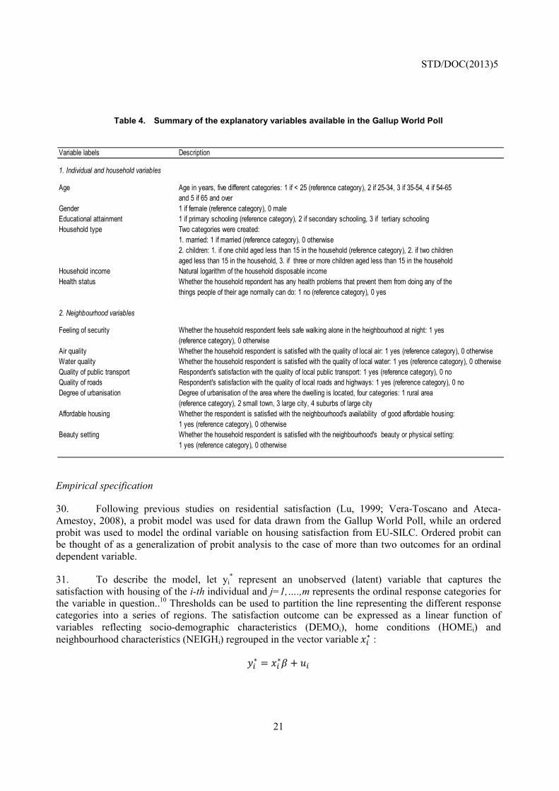
29. Table 3 and Table 4 describe the main features of the explanatory variables considered in the study, as available in the EU-SILC ad hoc module and in the Gallup World Poll respectively. Unfortunately, no information on housing conditions is available in the Gallup World Poll, which however includes a few variables on households’ perceptions of their neighbourhoods.

STD/DOC(2013)5

20

Table 3. Summary of explanatory variables available in EU-SILC

Variable labels Description

1. Individual and household variables

Age

Gender 0 if male, 1 if female (reference category)Educational attainment

Household type Four categories were created:1. married: 1 if married (reference category), 0 otherwise2. single: 1 if one person household (reference category), 0 otherwise3. lone parents: 1 if one single parent with one or more children (reference category), 0 otherwise

Household income Natural logarithm of the equivalised household disposable incomeHealth status

2. Housing variables

Tenure

Housing costs Ratio of total housing costs over equivalised household disposable incomeHousing burden

Dwelling type Four categories: 1 if detached house (reference category), 2 if semi-detached house, 3 if apartment in building with less than 10 dwellings, 4 if apartment in building with 10 or more dwellings

Rooms per person Number of rooms per personShortage of space Respondent's perceptions of shortage of space in dwelling: 1 if yes (reference category), 0 otherwiseBath or shower Bath or shower in dwelling: 1 if yes (reference category), 0 otherwiseFlushing toilets Indoor flushing toilets in dwelling: 1 if yes (reference category), 0 otherwiseStructural damages

Electrical installations

Plumbing installations

Too dark Whether the household respondent perceives the dwelling as being too dark: 1 yes (reference category), 0 otherwiseComfortably warm

Heating facilities

3. Neighbourhood variables

Crime

Noise

Environmental problems

Access to grocery services

Access to public transport

Access to health care services

Degree of urbanisation Degree of urbanisation of the area where the dwelling is located, three categories: 1 densely populated area (reference category), 2 intermediate area, 3 thinly populated area

Whether, in the judgement of the household respondent, the dwelling has a problem with a leaking roof, damp ceilings, dampness in the walls, floors or foundation or rot in windowframes and doors: 1 if yes (reference category), 0 otherwiseWhether, in the judgement of the household respondent, the dwelling has adequate electrical installations: 1 if yes (reference category), 0 otherwiseWhether, in the judgement of the household respondent, the dwelling has adequate plumbing/water installations: 1 if yes (reference category), 0 otherwise

Whether the household respondent perceives the dwelling as being comfortably warm during winter time: 1 yes (reference category), 0 otherwiseDwelling equipped with adequate heating facilities: 1 if yes (central or other fixed facilities) (reference category), 0 otherwise

Whether the household respondent perceives crime as a problem in the neighbourhood: 1 yes (reference category), 0 otherwiseWhether the household respondent perceives noise from neighbours or the street as a problem: 1 yes (reference category), 0 otherwiseWhether the household respondent perceives pollution, grime or other environmental problems to be a concern for the household: 1 yes (reference category), 0 otherwiseRespondent's assessment of accessability to grocery services: 1 easy or very easy (reference category), 0 difficult or very difficultRespondent's assessment of accessability to public transport: 1 easy or very easy (reference category), 0 difficult or very difficultRespondent's assessment of accessability to primary health care services: 1 easy or very easy (reference category), 0 difficult or very difficult

Self-reported assessment of the extent to which housing costs are a financial burden, three categories: 1 a heavy burden (reference category), 2 somewhat a burden, 3 not burden at all

1 if pre-primary or primary schooling (reference category), 2 if lower secondary and secondary schooling, 3 if post-secondary and tertiary schooling

Age in years, five different categories: 1 if < 25 (reference category), 2 if 25-34, 3 if 35-54, 4 if 54-65 and 5 if 65 and over

Self-reported health status, three different categories: 1 if very bad or bad (reference category), 2 if fair, 3 if good or very good

4. children: 1 if two adults and one dependent child (reference category), 2 if two adults and two dependent children, 3 if two adults and three or more dependent children

Four categories: 1 if owner (reference category), 2 if tenant paying rent at market rate, 3 if accomodation rented at a reduced rate, 4 if accomodation provided for free

STD/DOC(2013)5

21

Table 4. Summary of the explanatory variables available in the Gallup World Poll

Empirical specification

30. Following previous studies on residential satisfaction (Lu, 1999; Vera-Toscano and Ateca-Amestoy, 2008), a probit model was used for data drawn from the Gallup World Poll, while an ordered probit was used to model the ordinal variable on housing satisfaction from EU-SILC. Ordered probit can be thought of as a generalization of probit analysis to the case of more than two outcomes for an ordinal dependent variable.

31. To describe the model, let yi* represent an unobserved (latent) variable that captures the

satisfaction with housing of the i-th individual and j=1,….,m represents the ordinal response categories for the variable in question..10 Thresholds can be used to partition the line representing the different response categories into a series of regions. The satisfaction outcome can be expressed as a linear function of variables reflecting socio-demographic characteristics (DEMOi), home conditions (HOMEi) and neighbourhood characteristics (NEIGHi) regrouped in the vector variable ∗ : ∗ = ∗ +

Variable labels Description

1. Individual and household variables

Age

Gender 1 if female (reference category), 0 maleEducational attainment 1 if primary schooling (reference category), 2 if secondary schooling, 3 if tertiary schoolingHousehold type Two categories were created:

1. married: 1 if married (reference category), 0 otherwise

Household income Natural logarithm of the household disposable incomeHealth status

2. Neighbourhood variables

Feeling of security

Air quality Whether the household respondent is satisfied with the quality of local air: 1 yes (reference category), 0 otherwiseWater quality Whether the household respondent is satisfied with the quality of local water: 1 yes (reference category), 0 otherwiseQuality of public transport Respondent's satisfaction with the quality of local public transport: 1 yes (reference category), 0 noQuality of roads Respondent's satisfaction with the quality of local roads and highways: 1 yes (reference category), 0 noDegree of urbanisation

Affordable housing

Beauty setting

Degree of urbanisation of the area where the dwelling is located, four categories: 1 rural area (reference category), 2 small town, 3 large city, 4 suburbs of large cityWhether the respondent is satisfied with the neighbourhood's availability of good affordable housing: 1 yes (reference category), 0 otherwise

Whether the household respondent feels safe walking alone in the heighbourhood at night: 1 yes (reference category), 0 otherwise

Whether the household respondent is satisfied with the neighbourhood's beauty or physical setting: 1 yes (reference category), 0 otherwise

Age in years, five different categories: 1 if < 25 (reference category), 2 if 25-34, 3 if 35-54, 4 if 54-65 and 5 if 65 and over

2. children: 1. if one child aged less than 15 in the household (reference category), 2. if two children aged less than 15 in the household, 3. if three or more children aged less than 15 in the household

Whether the household repondent has any health problems that prevent them from doing any of the things people of their age normally can do: 1 no (reference category), 0 yes

STD/DOC(2013)5

22

where ~ (0, 1), ∀ = 1,… . , and β is a vector of unknown parameters. It is assumed that yi* is related

to the observable ordinal variable yi and that it takes values 0 through m (the highest ordinal category) according to the following scheme: = 0 [“very dissatisfied”] if -∞ < θ0 = 1 [“dissatisfied”] if θ0 ≤ ∗ < θ1 = 2 [“satisfied or very satisfied”] if ∗ ≥ θ1

or, more generally: = ⇔ < ∗ ≤

Ordered probits, like models for binary data, are meant to explain how changes in the predictors translate into changes in the probability of observing a particular ordinal outcome. In general terms, it is straightforward to see that: [ = ] = − − − for = 1,… . ,

where (. ) denotes the cumulative distribution function operator for the standard normal. As a maximum likelihood method is used to estimate the parameter vector, a general expression for the log-likelihood function needs to be specified:

ln = δ ln[ − − − ] where δ = 1if the i-th individual’s response fall within the j-th category and 0 otherwise. As it stands, optimization of this log-likelihood will not result in a unique solution. To get around this problem, an identification constraint is set on the parameter θ0, such that = 0. Moreover, as in the standard probit, the normalisation that = 1 is also imposed. This restriction, which is reflected in the assumption made for , arbitrarily fixes the scale of the latent dependent variable. To control for specific country-effects dummy variables for each country were also introduced.

Results

32. This section presents and discusses the results of a multivariate analysis aiming at gauging the effects of socio-demographic characteristics as well as house- and neighbourhood-related variables on people’s housing satisfaction. Results are described separately for the analysis based on the EU-SILC ad hoc module, limited to European countries; and for the analysis based on the Gallup World Poll, which refers to a broader range of countries but is based on a more narrow set of explanatory variables.

33. Table 5 shows estimates of the marginal effects of the independent variables on the probability of being satisfied or very satisfied with the dwelling where respondents live, based on the ordered probit analysis carried out on data drawn from the EU-SILC ad hoc module.11 Estimates, which are presented separately for Western- and Eastern-European countries, highlight a number of patterns.

• As for socio-economic and demographic characteristics, the coefficients on age mimic the findings of previous research, i.e. there is a U-shaped relationship between age and housing satisfaction (see Van Praag et al., 2003), at least in Western-European countries where people

STD/DOC(2013)5

23

aged 25-34 are less likely to be satisfied with housing than older cohorts. This difference in housing satisfaction between people of different ages is likely to be related to changes in family structure, as respondents aged between 25 and 34 are more likely than other people to envisage changes in their family composition. Housing needs – and hence satisfaction – are likely to change over the course of a household’s life-cycle, as during the child-rearing stage household size increases, and so does density in the house. The lower well-being for these households in Western-European countries implies that households that are entering the child-rearing stage are more likely to be dissatisfied with their dwelling than other population groups, while people aged 65 and over are more likely to be satisfied with their house than other cohorts, probably because of the smaller household size and higher home ownership rates in old age. There is no U-shaped relationship between age and housing satisfaction in Eastern-European countries.

• In regard to the effect of the household composition, single-parent headed households experience lower levels of housing satisfaction. The possible explanation behind this result is twofold. First, single-parent headed households often face tight budget constraints and economic hardship that force them into more crowded, less desirable housing that they would prefer. Second, single-parent households tend to express lower levels of subjective well-being, which might in turn translate into lower levels of housing satisfaction.12

• Couples with two dependent children or more are more dissatisfied with housing, which suggests that housing satisfaction declines as the number of people in the dwelling increases. This may be explained in terms of shortage of space: a couple with two or more children will have different needs in terms of available space than a couple with one child.

• Education does not have a significant role in shaping housing satisfaction across Europe. However, household income seems to have a significant, although small, effect on housing satisfaction, with high-income households being more satisfied with their dwelling than low-income ones.

• There are no significant differences in housing satisfaction by gender; however, marital status seems to play a role, with married individuals in Eastern-European countries more satisfied with their dwellings than their single counterparts.

STD/DOC(2013)5

24

Table 5. The determinants of housing satisfaction in European countries: analysis based on the EU-SILC ad hoc module on housing

Marginal effects of explanatory variable on the probability of being satisfied or very satisfied with housing

Note: *** Statistically significant at 1% confidence level, ** Statistically significant at 5% confidence level, * Statistically significant at 10% confidence level.

Source: OECD calculations based on data from EU-SILC, 2007.

Individual and houseold variables

Age 25-34 -0.0052* -0.0047Age 35-54 0.0038 0.0037Age 55-64 0.0049 0.0046Age 65 and over 0.0143* 0.0126

Female -0.0160 -0.0166

Married 0.0027 0.0444*

Secondary education -0.0111 -0.0087Tertiary education -0.0123 -0.0113

Household disposable income (ln) 0.0452** 0.0302*

Fair health status 0.0121 0.0118Good or very good health status 0.0281 0.0276

Single-headed households -0.0348 -0.0460Single-parent household -0.0613* -0.0619*2 parents - 1 child -0.0423 -0.0406*2 parents - 2 children -0.0718** -0.0669**2 parents- 3 or more children -0.0924** -0.0869**

Housing costs and characterisitcs

Tenant paying rent at market rate -0.3872*** -0.3806***Tenant paying rent at reduced rate -0.3990*** -0.3962***Tenant not paying any rent -0.1200*** -0.1179***

Total housing costs over income -0.0032*** 0.0007

Housing costs are slight burden 0.1563*** 0.1482***Housing costs are not a burden 0.1849*** 0.1691***

Semi-detached house -0.0729* -0.3806***Apartment in building with < 10 flats -0.0466* -0.3962***Apartment in building with > 10 flats 0.0135 -0.1179***

Number of rooms per person 0.0670*** 0.0701***

Shortage of space -0.4739*** -0.4761***

Indoor bath or shower 0.1699*** 0.1731***

Indoor flushing toilets -0.0564 -0.0537

Structural damages -0.1556*** -0.1551***

Adequate electricity installations 0.3250*** 0.3261***

Adequate plumbing installations 0.3044*** 0.3056***

Adequate heating facilities 0.1217*** 0.1258***

Comfortably warm 0.1432*** 0.1432***

Too dark -0.2937*** -0.2952***

Neighbourhood characteristics

Intermediate populated area -0.0734** -0.0752**Thinly populated area 0.0554** 0.0524**

Crime is a problem in the neighbourhood -0.1457*** -0.1449***

Environment is a problem in the neighbourhood -0.0831*** -0.0823***

Noise is a problem in the neighbourhood -0.0846*** -0.0843***

Access to grocery services 0.1125*** 0.1117***Access to public transport 0.0194 0.0201Access to health care services 0.1100*** 0.1113***

θ0 -0.4506** -0.5837***

θ1 0.4972*** 0.3637*

Observations 118,226 55,960

Western-European countries Eastern-European countries

STD/DOC(2013)5

25

• Home ownership appears to be one of the main drivers of housing satisfaction, a result that is in line with the previous literature. Home ownership is likely to boost housing satisfaction through direct and indirect channels. Owning a house is not only a way to store and build wealth and enjoy freedom and control over improvements and upgrades to the dwelling, but it also produces a set of positive externalities – ranging from investing in social relationships with the neighbours to being more active in local politics and neighbourhood organisations.

• Housing costs as a percentage of household disposable income, and household perceived burden, are also important factors: households who do not perceive housing costs as a heavy burden are more satisfied with their dwellings than households for whom these costs turn out to be heavy.

• Structural and qualitative features of the dwelling are very important in determining housing satisfaction. Living in a detached house, with adequate electricity and plumbing installations, equipped with heating facilities that keep the dwelling comfortably warm during winter time, are all requisites to enjoy higher levels of housing satisfaction. On the contrary, shortage of space, structural damages (e.g. leaking roofs, damp ceilings and dampness in the walls), the lack of indoor showers or flushing toilets and a dark home environment are all elements that have strong and negative effects on households’ satisfaction with their dwellings.

• Neighbourhood characteristics are strong determinants of housing satisfaction. Households who live in less populated areas, free from crime, environmental problems13 and noise, and that benefit from easy access to grocery services and primary health-care services are more likely to experience higher levels of housing satisfaction than their counterparts living in more populated or disadvantaged neighbourhoods.

• Country dummy variables (not reported in Table 6 due to space limitations) show large and significant differences in housing satisfaction across Eastern- and Western-European countries after controlling for a range of individual and residential characteristics. As for East European countries, the probability of experiencing high housing satisfaction is highest in the Czech Republic, while it is lowest in Lithuania and Estonia and in the medium range in Latvia and Poland. Among West European countries, the level of housing satisfaction is highest in Sweden, Luxembourg and Austria, while it is lowest in Germany and Ireland and exhibits intermediate values in France, Greece and Spain.14

34. Table 6 summarises the results from analysis based on the Gallup World Poll. Estimates are based on a probit model, and are shown separately for OECD countries and other major economies. Most of the patterns highlighted by these data mirror those for European countries, based on EU SILC, although some differences emerge:

• Women are more likely to express high levels of housing satisfaction than men, a result that holds only in OECD countries.

• Housing satisfaction increases with educational attainments in both OECD and other major economies, yet the effect is significant only for people with tertiary education in OECD countries and for people with secondary education in emerging economies.

• Housing satisfaction also increases with income, although this effect is weaker in OECD than in emerging countries.

STD/DOC(2013)5

26

• In emerging countries, households with one child or more are more likely to report lower levels of housing satisfaction than households without children, a result that does not hold in OECD countries.

• As for the neighbourhood characteristics, households living in a small city or in the suburbs of a big city are more likely to experience lower levels of housing satisfaction than their counterparts living in rural areas or villages.

• Availability of affordable dwellings in the neighbourhood increases the overall residential satisfaction in both OECD countries and other major economies.

• Households who feel safe when walking alone in the neighbourhood at night as well as those who are satisfied with the quality of the local environment are also more likely to be satisfied with their dwelling. Access to public transport and beauty settings are also strong determinants of housing satisfaction in OECD countries.

• Estimates of country fixed-effects (not shown in Table 6) confirm large and significant variation among OECD countries and other major economies. In the OECD area, households living in Belgium, Portugal, Sweden and Australia are more likely to report high levels of housing satisfaction, while in Chile, Japan and Estonia satisfaction with the conditions of dwellings and neighbourhoods appears to be significantly lower.

STD/DOC(2013)5

27

Table 6. The determinants of housing satisfaction in OECD and partner countries: analysis based on the Gallup World Poll

Marginal effects of the explanatory variables on the probability of being satisfied with housing

Note: *** Statistically significant at 1% confidence level, ** Statistically significant at 5% confidence level, * Statistically significant at 10% confidence level.

Source: OECD calculations based on data from the Gallup World Poll, 2005, 2006 and 2007.

Individual and household characteristics

Age 25-34 -0.0327* -0.0292Age 35-54 -0.0239 0.0079Age 55-64 0.0180 0.0789Age 65 and over 0.0645** -0.0013

Female 0.0322** 0.0051

Married 0.0002 -0.0281

Secondary education 0.0105 0.0368*Tertiary education 0.0719*** 0.0227

Household disposable income (ln) 0.0138** 0.0817***

Health problems -0.0144 -0.0300

One child -0.0079 -0.0755**Two children -0.0234 -0.0643**Three children or more -0.0348 -0.0174

Neighborhood characteristics

Small city -0.0432* 0.1132**Big city -0.0277 0.0005Suburbus of a big city -0.0562** 0.0126

Housing affordability 0.1471*** 0.1135***

Beauty setting 0.0571*** 0.0439

Feeling of security 0.0574*** 0.0783*

Satisfaction with local air quality 0.0216* 0.0207Satisfaction with local water quality 0.0072* 0.0632**

Access to roads 0.0084 -0.0020Access to public transport 0.0531*** -0.0180

Observations 11,061 4,652

OECD countries Other major economies

STD/DOC(2013)5

28

35. By and large, the results of the multivariate analysis based on both EU-SILC and the Gallup World Poll confirm that housing satisfaction responds to complex dynamics, influenced by both housing characteristics and neighbourhood’s features and mediated by individual and household characteristics.

Conclusion

36. By taking advantage of two household surveys (the EU-SILC ad hoc module on housing for European countries; and the Gallup World Poll for OECD countries and other major economies), this paper has explored the link between households’ residential satisfaction and a number of variables related to individuals, the households to which they belong, and the characteristics of the dwelling and neighbourhood where they live. The main result of this analysis is that residential satisfaction is shaped by both housing characteristics and neighbourhood’s features. Individual and household socio-demographic characteristics (e.g. age, gender, education) play a secondary role once dwelling and neighbourhood features are controlled for.

37. In European countries, four factors can be identified as major predictors for households’ residential satisfaction: tenure, specific dwelling features (i.e. shortage of space, inadequate electricity and plumbing installations and a dark home environment), the financial burden of housing costs, and perceived level of crime in the neighbourhood. In addition to these factors, the type of dwelling has a significant effect on residential satisfaction in Eastern-European countries.

38. In OECD countries, housing affordability is the main driver of residential satisfaction. Neighbourhood characteristics such as beauty setting, access to public transports and the feeling of security also exert a positive, significant effect. The strong effect of housing affordability is confirmed also by the analysis carried out on other major economies.

39. Another interesting pattern emerging from this study concerns the impact of household income on residential satisfaction. This effect (in the Gallup World Poll data) tends to be weaker in OECD countries than in other major economies. The aspiration-gap approach may partially account for the result: in other words, once basic needs (such as being sheltered) are fulfilled, households expect higher living standards (such as living in a ‘pleasant’ area). This may explain why some neighbourhoods’ characteristics play a more important role in OECD countries than in other major economies.

40. Residential satisfaction is thus the result of how individuals perceive salient attributes of their physical environment and their consequent evaluation according to certain standards of comparison. Understanding the levers of residential satisfaction is important for any public policy aiming at enhancing people’s housing opportunities. The results presented in this paper support a menu of policy options ranging from programmes that ameliorate the structural features of dwellings, to policies that promote homeownership and facilitate the access to affordable housing for low-income households.

41. However, caution is warranted in the interpretation of results. Most of the patterns described above hold only for European countries, as no core sets of comparable housing indicators (including the tenure status and the physical attributes of the dwelling) exist for non-European countries. Further research would benefit from the inclusion of questions on such variables into the surveys used in non-European countries.

42. Moreover, country dummy variables indicate large and significant variation in residential satisfaction across countries. This finding suggests the need to further investigate the levers of residential satisfaction at the country level by taking advantage of national datasets and surveys.

STD/DOC(2013)5

29

ANNEX A: THE DETERMINANTS OF SATISFACTION WITH LOCAL ENVIRONMENTAL QUALITY

43. The analysis in this paper suggests that people’s feeling with respect to the quality of the natural environment affect their residential satisfaction. However, satisfaction with environmental quality also reflects the impacts of a range of other characteristics. The analysis in this Annex provides evidence of the type of factors that are at work.

44. Pollution of air and other environmental media is not evenly distributed, and existing measures can be mapped to describe how this relates spatially to population characteristics (King and Stedman, 2000). Such techniques however tell little about how air pollution is experienced by people. Form both an analytic and policy perspective, it is important to know how social and geographical influences may impact on such perceptions and related concerns. Early works explored some possibilities, with mixed result; some authors suggested that habituation could occur following higher or longer exposure, though others did not; other authors reported that environmental concerns where higher among people from higher socio-economic status. For example, Bickerstaff and Walker (2001) report an inverse relationship between socio-economic status and concern for air quality, suggesting that this reflect differences in environmental quality, and a reluctance to recognise negative conditions in localities where satisfaction is high. Elliot et al. (1999) find that the presence of other social problems in the neighbourhood could lead to less importance being ascribed to air pollution.

45. Table A.1 below reports results of a multivariate analysis on the determinants of people’s satisfaction with air and water quality, based on a selection of socio-economic variables available in the Gallup World Poll. This analysis is related to the work of Silva et al. (2012), although it differs from that in some respects. First, this analysis is meant to explore the drivers of people’s satisfaction with both air and water quality. Second, the effect of environmental quality on subjective well-being is not investigated. However, most of the determinants of satisfaction with air quality shown below are in line with those in Silva et al. Results are shown separately for both OECD and major partner countries. Some of the main patterns include the following:

• The area where people live is the strongest predictor of perceptions of local environmental quality. In OECD countries, populations living in large cities or in their suburbs are significantly less satisfied than people living in rural areas or small towns. In major partner countries, this relation holds only for people living in big cities.

• More educated people are less satisfied with the quality of the local environment, a pattern that holds in both OECD and major partner countries. This result is in line with the existing research, which suggests that more educated people appreciate more the consequences of certain human effects on the environment, and that they can make a stronger connection between social welfare and the environment (Thalmann, 2004; Kahn and Matsusaka, 1997).

• Access to TV and the Internet (a proxy for media exposure) suggests that people who have access to a larger set of information on environmental hazards and their harmful effects on human health are less satisfied with the quality of local air and water.15

• Age also affects perceived environmental quality, although its effect is not strong: in OECD countries. Older people are less satisfied with air and water quality, possibly because they are likely to suffer from pre-existing respiratory or cardiovascular diseases, and to spend more time

STD/DOC(2013)5

30

outdoors. Similarly, gender seems to play a role in satisfaction with the local environment, with women significantly more dissatisfied than men, but only in OECD countries.

Table A.1. The determinants of satisfaction with environmental quality

Marginal effects of explanatory variables on satisfaction with air and water quality

Note: Probit analysis includes all OECD countries, Brazil, China, India, Indonesia, the Russian Federation and South Africa. * indicates that values are significant at the 10% confidence level; ** indicates that they are significant at the 5% confidence level; and *** indicates that they are significant at the 1% confidence level. A positive value means that the explanatory variable increases the propensity of satisfaction with an increase in its magnitude.

Source: OECD’s calculations based on Gallup World Poll, 2009 and 2010.

Satisfaction with air quality Satisfaction with water quality Explanatory variables OECD only BRICS only OECD only BRICS only Female -0.0282*** 0.0068 -0.0195** -0.0040 Age -0.0023* -0.0086 -0.0035*** -0.0021 Age squared 2.88 e-05* -3.82 e-06 0.0004*** 3 e-05 Log household income 0.0028 0.0023 0.0028 0.0070 Unemployed 0.0088 -0.1244*** -0.0292 -0.1004*** Secondary education -0.0311* -0.0586*** -0.0331*** -0.0457*** Tertiary education -0.0337* -0.0689*** -0.0184* -0.0642** Small town -0.0682*** -0.0404*** -0.0218 -0.0359 Big city -0.2066*** -0.1455*** -0.0622*** -0.0095** Suburb of a big city -0.1464*** -0.1217*** -0.0146 -0.0008 Number of children -0.0003 0.0004 -0.0010 0.0006 Access to TV 0.0207 -0.0699*** -0.0548** -0.0958*** Access to the Internet 0.0078 -0.0537*** -0.0326*** -0.0312*

STD/DOC(2013)5

31

ANNEX B: THE DETERMINANTS OF SELF-REPORTED VICTIMISATION AND THE FEELING OF SECURITY

46. People’s feelings with respect to the security of the local neighbourhood also shape their residential satisfaction. This annex provides evidence on the range of factors at work based on data from the Gallup World Poll.

47. Individuals have different exposures to risk of being victim of a crime. Victimisation surveys show that young people are at least as much at risk of victimisation as adults, and for some crimes even more at risk, irrespective of gender, class and location. Although it is generally assumed that the decline in physical resiliency that accompanies the ageing process increases vulnerability, the frequency of going out, which is related to age, is also relevant. Because of their lifestyle, younger people typically face a higher risk of being victims of criminal aggression. Moreover, official statistics and self-reported studies have consistently shown that men are at greater risk of being victims of assault and violent crimes than women, particularly with respect to offences by strangers and by other men (Carrabine et al., 2009). In the United States, minority groups also generally suffer from higher victimisation rates than whites. However, it is extremely difficult to isolate ethnicity as a single variable in explaining patterns of victimisation, as socio-economic factors may be at work as well. Ethnic minority groups are likely to live in socially disadvantaged areas, which place them at higher risk of victimisation (Modood et al., 1997).

48. Beyond demographic characteristics, research shows that some of the main socio-economic determinants of victimisation are: i) where people live; ii) whether they lead a risky lifestyle, including how much they go out at night; iii) how attractive they are as a target (e.g. whether they are perceived as vulnerable or they simply own valuable objects); iv) the extent of guardianship (e.g. the absence of a capable guardian or electronic security measures that can deter crime) (Carrabine et al., 2009). Survey data have highlighted the spatial concentration of crime victimisation in urban areas (as opposed to rural areas) and in poor areas (as opposed to wealthy areas): urban dwellers may live closer to high offending populations, and their daily routines tend to bring them into contact with each other in more anonymous settings (Lee, 2000; OECD, 2011c). Research also suggests that being married reduces the risk of being assaulted, a result that may reflect the effect of marriage in lowering risk-taking behaviour (e.g. going out at night, using public transport) and in strengthening social control (Umberson, 1987; Cheung; 1998). People with higher incomes and educational status usually face lower risks of crime (especially property crime), as they can afford better security and are less likely to associate with people from disadvantaged backgrounds, whose likelihood of being an offender is higher (Kelly, 2000). Finally, people with physical impairments or psychological distress are more likely to be victimised, as these conditions render them less capable of deterring crime and make them easier targets (Nosek et al., 2001; Marley and Buila, 2001).

49. People with different characteristics also report differentially in terms of fear of crime. Fear of crime varies according to gender and age of respondents, but also depends on their health, ethnicity, marital status and social class. Research has shown that women report lower feelings of security than men, which may reflect the effect of what researchers have called the “shadow of sexual assault” (Ferraro, 1995): women may be more fearful of being mugged than men because the incident may also lead to a sexual attack. Moreover, women may feel that they must protect not only themselves but also their children, or that they will be perceived as partially responsible (due to routine activities, clothing, etc.) if they are the victim of a personal crime (Schafer et al., 2006). While previous research highlighted elderly people as being the most fearful in society, recent studies have challenged this finding (Moore and Shepherd, 2007).16 People living in major cities or their suburbs are more concerned about crime than people living in small settlements or urban areas (Van Dijck and Smit, 2008). People in unskilled occupations are also more fearful than those in skilled occupations, while those who consider themselves

STD/DOC(2013)5

32

to be in poor health or with disability have higher concerns about crime (Stiles et al., 2003). Married people express lower fear of crime than their non-married counterparts, perhaps due to changes in lifestyle, as well as a decreased sense of vulnerability (Mesch, 2000). Similarly, social ties may reduce concerns about crime, as they provide a support structure for coping with crime and a sense of familiarity and control in the neighbourhood (Carrabine et al., 2009). Finally, several studies found an association between previous victimisation and fear of crime levels (Skogan, 1987).

50. Following the empirical approach taken by these various studies, an analysis of the main determinants of victimisation and feelings of security has been carried out based on the indicators from the Gallup World Poll (Table B.1.). The sample includes both OECD and major partner countries (Brazil, the Russian Federation, India, Indonesia and China). Most of the findings of this analysis are consistent with those from the research discussed above, although a few are not fully in line with the literature, thus suggesting the need for further research.

Table B.1. The determinants of self-reported assault and the feeling of security

Marginal effects of explanatory variables on self-reported victimisation and the feeling of security

Note: Probit analysis includes all OECD countries, Brazil, China, India, Indonesia, the Russian Federation and South Africa. * indicates that values are significant at 10% confidence level; ** indicates that they are significant at 5% confidence level; and *** that they are significant at 1% confidence level. A positive value in the left column means that the explanatory variable increases the likelihood of being victim of an assault, while a negative value in the right column means that the explanatory variable increases the likelihood of feeling safe when walking at night in the neighbourhood. The variable “household income” refers to the base-2 logarithm of the household disposable income.

Source: OECD Secretariat's calculations based on data from the Gallup World Poll.

51. The results shown in the left column of Table B.1 refer to self-reported assault and mugging victimisation. In line with previous research, people living in large conurbations and people reporting health problems (as measured by self-reports of poor health status17) experience higher levels of self-reported victimisation. Men and young people between the age of 16 and 24 face a higher risk of assault, while being married reduces that risk. Education does not seem to affect the risk of assault, unlike in previous studies where education was used as a proxy of the quality of neighbourhood where people live.18 Social ties are associated with lower victimization.19

52. The right column of Table B.1 shows the effect of different variables on the feeling of security. Previous victimisation is the strongest negative determinant. In line with previous research, women report lower feelings of security than man, despite being less likely to be victimised (see left column of Table

Explanatory variables Self-reported victimisation

Feeling of security

Female -0.0098*** -0.0135***Age 25-34 -0.0112*** 0.0280***Age 35-54 -0.0139*** 0.0342***Age 55-64 -0.0156*** 0.0385***Age 65+ -0.0196*** -0.0112Marital status -0.0042* 0.0100*Household income -0.0015* 0.0024Secondary education -0.0021 -0.0296***Tertiary education -0.0003 0.0191**Small town 0.0071** -0.0601***Big city 0.0199*** -0.1144***Suburb of a big city 0.0036 -0.0748***Poor health status 0.0194*** -0.0289***Perceived social network -0.0050* 0.0757***Previous victimisation -0.1878***

STD/DOC(2013)5

33

B.1.). One possible explanation of this relationship is that the fear of crime leads women to change their routines, thus avoiding certain areas and people. Young people are also more fearful (and more likely to be assaulted, see left column of Table B.1.) than those between 25 and 64 years old. Married people and those who have relatives or friends they can count on in case of trouble (as proxied by the variable “perceived social network”) feel safer when walking alone at night in their neighbourhood. People living in large cities are significantly more fearful than their counterparts living in rural or small settlements. Education has an ambiguous effect on fear of crime, as people with higher education report higher feelings of security than individuals with primary education; however, people with upper-secondary education report lower feelings of security than individuals with primary education. Contrary to previous research, income does not seem to influence people’s feeling of security; one possible explanation may be that the variable used in this analysis is measured at the level of the household rather than the individual, and that the latter is in principle a more powerful predictor of fear of crime. Living in cities or suburbs (as opposed to living in rural areas) increases fear of crime while a stronger perceived social network decreases it.

53. Given the methodological limitations outlined above and considering that some of the results contradict previous research, this analysis needs to be corroborated by further research. In addition, the analysis would benefit from the consideration of more detailed individual and risk-related variables (e.g. risky lifestyle, ethnicity, satisfaction with the neighbourhood and the police).

NOTES

1 . Financial affordability of housing “is concerned with securing some given standard of housing (or

different standards) at a price or a rent which does not impose, in the eyes of some third party (usually government), an unreasonable burden on household incomes” (Maclennan and Williams, 1990, as quoted in Hui, 2001). Based on the notion of financial affordability, the concept of housing availability refers to the number of housing units that are affordable to households within a certain income group.

2. There is an extensive literature devoted to the concept of affordability of both owner-occupied and rental housing (Whitehead et al., 2009). The starting point for affordability analysis is a normative judgement about the costs of living in an “adequate” dwelling and the income that needs to be left over to meet other non-housing requirements. There are two types of affordability measures used: the first is based on the ratio of housing costs to income; the second is based on the residual income remaining after meeting housing costs. The former approach allows the researcher to identify the proportion of income that should not be exceeded when paying for a home of adequate size and quality. The latter is tied to an assessment of whether the income left over after paying for a decent home is sufficient to allow a “reasonable” standard of living. In both approaches, measures of housing affordability may vary depending on how housing costs and household income are defined. Housing costs may be limited to outlays for rent (in the case of households renting their main residence), or include expenditures on energy or other services connected with housing (repair, utilities); in the case of households who own their main residence, these costs may include the repayment of loans secured to purchase or maintain housing. Household incomes can also be calculated as gross or net (i.e. after taxes and other mandatory insurance payments).

3 . The model presented in this section is similar to that proposed by Amole (2009).

4 . In the analysis presented in this paper, Eastern European countries include the Czech Republic, Estonia, Hungary, Latvia, Lithuania, Poland, Slovakia and Slovenia. Western European countries refer to: Austria, Belgium, Cyprus, Germany, Denmark, Spain, Finland, France, Greece, Ireland, Iceland, Italy, Luxembourg, the Netherlands, Norway, Portugal, Sweden and the United Kingdom.

STD/DOC(2013)5

34

5 . Other major economies are China, India, Indonesia, the Russian Federation and South Africa. Micro data

from the Gallup World Poll were made available courtesy of Gallup Europe.

6. To measure residential satisfaction, some authors have used several highly correlated items rather than a single-item variable. Francescato et al. (1989) suggested to measure residential satisfaction through a list of four questions: i) how satisfied are you with living here? ii) how long do you want to live in this housing development? iii) if you move again would you like to live in another place like this? iv) would you recommend this place to one of your friends if they were looking for a place to live? Based on the theoretical contribution by Francescato et al., Carvalho et al. (1997) used a similar list of variables and suggested that conceiving residential satisfaction as a multifaceted construct increases the reliability of the measure. However, other authors criticise the use of a composite indicator, as its construction is not straightforward and often involves a number of steps (e.g., aggregation, weighting) that need to be carefully examined. For these reasons and data availability constraints, this study relies on a single-item variable measuring housing satisfaction.

7 . As for the household composition, EU-SILC defines ‘dependent children’ as household members aged less that 18 and those aged between 18 and 24 who are economically inactive and living with at least one parent. The Gallup World Poll refers only to children under 15 years of age living in the household.

8. EU-SILC defines a room as a space of a housing unit of at least 4 square meters such as normal bedrooms, dining rooms, living rooms and habitable cellars and attics with height over 2 meters and accessible from inside the unit. Kitchens, bathrooms, toilets, corridors, utility rooms and lobbies are not counted as rooms. The variable “number of rooms per person” has been obtained by dividing the total number of rooms available to the household by the household size. A person is said to live in an overcrowded dwelling if the number of rooms available is less than: one room in the case of single-person household; one room per couple in the household; one room for each single person aged 18 or more; one room per pair of single people of the same gender between 12 and 17 years of age; one room per each single person between 12 and 17 years of age and not included in the previous category; one room per pair of children under 12 years of age (OECD, 2011).

9 . Total housing costs as a percentage of household disposable income (HCR) was calculated as the ratio of housing costs, net housing allowances received by households in the reference year, over the equivalised household disposable income, net housing allowances received in the same period. In order to adjust for the effect on the mean of extreme values, which may arise from unusual household circumstances or from errors in the data collected, in cases where housing costs exceed the equivalised household disposable income, HRC has been set equal to disposable income, net housing allowances; in cases where the housing costs are negative, the HRC has been set equal zero.

10. The binomial probit model can be viewed as a special case of the ordered probit where m=1.

11 . Marginal effects measure the impact of a unit change in each explanatory variable on the probability of being ‘satisfied or very satisfied’ with housing. The marginal impact of each independent variable is calculated while holding constant all other independent variables at their mean levels.

12 . Frey and Stutzer (2000), for instance, have shown that children generally affect well-being more negatively for single parents than for couples, while Schoon et al. (2005) have found a similar effect on the well-being of divorced mothers.

13 . As environmental problems and perceived levels of crime are among the determinants of residential satisfaction, it is important - from a policy perspective - to better understand what drives people’s satisfaction with the local environment and perceptions of crime. For a detailed analysis of the determinants of satisfaction with the local environmental quality, see Annex A. Annex B shows the results of a multivariate analysis on the determinants of self-reported victimisation and the feeling of security.

14 . The full set of results is available from the authors upon request.

STD/DOC(2013)5

35

15 . The variable “access to TV” is based on the following question in the Gallop World Poll: “Does your home

have a television?” Similarly, the variable “access to the Internet” is based on the following question: “Does your home have access to the Internet?”

16 . As fear of crime is a complex construct, recent research has recognised that relative levels of fear of crime may differ depending on different types of crime. Specifically, fear of personal victimisation appears to be related to being younger. According to Moore and Shepherd (2007), fear of personal victimisation was highest among those aged 16 to 25. By contrast, fear of property victimisation was associated with the middle-age years and was highest among those aged 40 to 60.

17. The variable “poor health status” is based on the following Gallup question: “Do you have any health problems that prevent you from doing any of the things people your age normally can do?

18 . Education may perform as a poor proxy of neighbourhood in the analysis shown here, or its effects may be captured by income, which controls in principle for similar factors.

19. The variable “perceived social network” is built upon the following Gallup question: “If you were in trouble, do you have relatives or friends you can count on to help you whenever you need them, or not?”

STD/DOC(2013)5

36

REFERENCES

Alber, J. and T. Fahey (2004), Perceptions of living conditions in an enlarged Europe (consolidated report), European Foundation for the Improvement of Living and Working Conditions, Dublin.

Amerigo, M. and J. I. Aragones (1997), “A theoretical and methodological approach to the study of residential satisfaction”, Journal of Environmental Psychology, 17/1, pp. 47-57.

Amole, D. (2009), “Residential satisfaction in students’ housing”, Journal of Environmental Psychology, Vol. 29, pp. 76-85.

Andrews, D. and A. Caldera Sánchez, (2011), “Drivers of Homeownership Rates in Selected OECD Countries”, OECD Economics Department Working Papers, No. 849, OECD Publishing, Paris.

Aneshensel, C. S. and C. A. Sucoff (1996), “The neighbourhood context of adolescent mental health”, Journal of Health and Social Behavior, Vol. 37, No.4, pp. 293-310.

Bickerstaff, K. and G. Walker (2001), “Public understandings of air pollution: The ‘localisation’ of environmental risk”, Global Environmental Change, Vol. 11, pp. 133-145.

Bogdon, A. and A. Can (1997), “Indicators of local housing affordability: Comparative and spatial approaches”, Real Estate Economics, 25/1, pp. 43-80.

Brower, S. (1996), Good Neighborhoods: A Study of In-Town and Suburban Residential Environments, Praeger, Westport, CT.

Bruning, S. D., A. Langehop and K. A. Green (2004), “Examining city-resident relationships: linking community relations, relationship building activities, and satisfaction evaluations”, Public Relations Review, Vol. 30, pp. 335-345.

Burke, T. and L. Ralston (2003), Analysis of Expenditure Patterns and Levels of Household Indebtedness of Public and Private Rental Households, 1975 to 1999, Final Report, Australian Housing and Urban Research Institute, Melbourne.

Canter, D. and K. Rees (1982), “A multivariate model of housing satisfaction”, Applied Psychology, Vol. 31, No. 2, pp. 185-207.

Carrabine, E., P. Iganski, L. Maggy, K. Plummer and N. South (2009), Criminology: A Sociological Introduction, Routledge, New York.

Carvalho, M., V. R. Goerge and K. H. Anthony (1997), “Residential satisfaction in conominos exclusivos (gate-guarded neighborhoods) in Brazil”, Environment and Behavior, No. 29, pp. 734-768.

Cheung, Y. B. (1998), “Accidents, Assaults, and Marital Status”, Social Science & Medicine., Vol. 47, No. 9, pp. 1325-1329.

Chuang, Y., C. Cubbin, D. Ahn and M. A. Winkleby (2005), “Effects of neighbourhood socioeconomic status and convenience store concentration on individual level smoking”, Journal of Epidemiology and Community Health. Vol. 59, pp. 568–573.

STD/DOC(2013)5

37

Clark, A. E. and A. J. Oswald (2002), “Well-being in panels”, mimeo, DELTA, Paris, France.

Coulton, C. J., J. Korbin, T. Chan and M. Su (2001), “Mapping residents’ perceptions of neighborhood boundaries: A methodological note”, American Journal of Community Psychology, Vol. 29, No. 2, pp. 371-383.

Crowley, S. (2003), “The affordable housing crisis: Residential mobility of poor families and school mobility of poor children”, Journal of Negro Education, 72/1, pp. 22-38.

Day, R. (2007), “Place and the experience of air quality”, Health & Place, Vol. 13, pp. 249-260.

Department for Communities and Local Government (2007), Homes for the future: more affordable, more sustainable, Green Paper Presented to Parliament by The Secretary of State for Communities and Local Government by Command of Her Majesty, London: The Stationery Office.

Diaz-Serrano, L. (2009), “Disentangling the housing satisfaction puzzle: Does homeownership really matter?”, Journal of Economic Psychology, 30/5, pp. 745-755.

Dietz, R. D. and D. R. Haurin (2003), “The Social and Private micro-level consequences of homeownership”, Journal of Urban Economics, Vol. 54, pp. 401-450.

Diez Roux, A. V., S. S. Merkin, D. Arnett, L. Chambless, M. Massing, F. Nieto, P. Sorlie, M. Szklo, H. Tyroler, and R. Watson (2001), “Neighborhood of residence and incidence of coronary heart disease”, New England Journal of Medicine, Vol. 345, pp. 99-106.

DiPasquale D. and E. L. Glaeser (1999), “Incentives and Social Capital: Are Homeowners Better Citizens?”, Journal of Urban Economics, Vol. 45, pp. 354-384.

Dolan, P., T. Peasgood and M. White (2008), “Do we really know what makes us happy? A review of the economic literature on the factors associate with subjective well-being”, Journal of Economic Psychology, Vol. 29, No.1, pp. 94-122.

Dunn, J. R. (2000), “Housing and health inequalities: Review and prospects for research”, Housing Studies, Vol. 15, No. 3, pp. 341-366.

Dunn, J. R. and M. V. Hayes (2000), “Social inequality, population health, and housing: a study of two Vancouver neighbourhoods”, Social Science and Medicine, Vol.51, No. 4, pp. 563-87.

Elliot, S., D. Cole, P. Krueger, N. Voorberg and S. Wakefield (1999), “The power of perception: Health risk attributed to air pollution in an urban industrial neighbourhood”, Risk analysis, Vol. 19, pp. 621-634.

Elsinga, M. and J. Hoekstra (2005), “Homeownership and housing satisfaction”, Journal of Housing and the Built Environment, Vol. 20, No. 4, pp. 401-424.

Environmental Protection Agency (2006), Healthy Homes, www.epa.gov/region1/healthyhomes/pdfs/healthyhomes.pdf.

Evans, G.W. (2006), “Child Development and the Physical Environment”, Annual Review of Psychology, No. 57, pp. 423-451.

STD/DOC(2013)5

38

Ferraro, K. F. (1995), Fear of Crime: Interpreting Victimisation Risk, State University of New York Press, Albany.

Freeman, L. (1998), “Interpreting the Dynamics of Public Housing: Cultural and Rational Choice Explanations”, Housing Policy Debate, Vol. 9, No. 2, pp. 323–353.

Freeman, A., C. Kiddle, and C. Whitehead (2000), “Defining affordability” in Monk, S. and Whitehead, C. (eds.) Restructuring Housing Systems: From Social to Affordable Housing?, York Publishing Services, York, pp. 42-49.

Frey, B. S., and A. Stutzer (2000), “Happiness, economy and institutions”, The Economic Journal, Vol. 110, pp. 918-938.

Francescato, G., S. Weidemann and J. R. Anderson (1989), “Evaluating the built environment from the users point of view: An attitudinal model of residential satisfaction” in W.F.E. Preiser (Ed.), Building evaluation, pp. 181-198, Plenum Press, New York.

Gabriel, M, et al. (2005), “Conceptualising and measuring the housing affordability problem”, Research Paper 1 for National Research Venture 3: Housing affordability for Lower Income Australians, Melbourne, Australian Housing and Urban Research Institute.

Galster, G. (1987). “Identifying the correlates of dwelling satisfaction: an empirical critique”, Environment and Behavior, Vol. 19, pp. 539-568.

Galster, G. (2001), “On the nature of neighborhood”, Urban Studies, 38/12, pp. 2111-2124.

Glass, R. (1948), The Social Background of a Plan: A Study of Middlesbrough, Routledge and Kegan Paul, London.

Grannis, R. (2003), “Islands in the city: Social networks and street networks”, Working paper, Department of Sociology, University of California, Los Angeles.

Guo, J. Y. and Ch. R. Bhat (2007), “Operationalizing the Concept of Neighborhood: Application to Residential Location Choice Analysis”, Journal of Transport Geography, 15/1, pp. 31-45.

Grzeskowiak, S., M. J. Sirgy and R. Widger (2003), “Residents’ Satisfaction with Community Services: Predictors and Outcomes”, Journal of Regional Analysis and Policy, Vol. 33, No. 2, pp. 1-36.

Hartman, C., and T. M. Franke (2003), “Student mobility: How some children get left behind”, Journal of Negro Education, Vol. 72, No. 1, pp.1-5.

Healy, J. D. (2004), Housing, Fuel Poverty and Health: A Pan-European Analysis, Ashgate Publishing Limited, Aldershot, England.

Hills, J., F. Hubert, H. Tomann and C. Whitehead (1990), “Shifting subsidy from bricks and mortar to people: Experiences in Britain and West Germany”, Housing Studies, Vol.5, No.3, pp. 147-167.

Hui, C. M. E. (2001), “Measuring Affordability in Public Housing from Economic Principles: Case Study of Hong Kong”, Journal of Urban Planning and Development, Vol. 127, No. 1, pp. 34-49.

Hur, M. and H. Morrow-Jones (2008), “Factors that Influence Residents’ Satisfaction with Neighbourhoods”, Environment and Behavior, Vol. 40, pp. 619-635.

STD/DOC(2013)5

39

James, R. N. (2007), “Multifamily housing characteristics and tenant satisfaction”, Journal of Performance of Constructed Facilities, 21/6, pp. 472-480.

Kahn, M. E. and J. G. Matsusaka (1997), “Demand for Environmental Goods: Evidence from Voting Patterns on California Initiatives” Journal of Law & Economics, 40/1, pp. 137–173.

Kelly, M. (2000), “Inequality and crime”, The Review of Economics and Statistics, Vol. 82, No. 4, pp. 530-539.

Kiel, K. A. and P. Mieszkowski, (1990), “An examination of systemic differences in the appreciation of individual housing units”, Journal of Real Estate Research, Vol. 5, pp. 301–318.

King, K. and J. Stedman (2000), Analysis of air pollution and social deprivation, AEA Technology Environment report AEAT/R/ENV/0241.

Krieger, J. and D. L. Higgins (2002), “Housing and Health: Time Again for Public Health Action”, American Journal of Public Health, 92/5, pp. 758-768.

Knox, P. and S. Pinch (2000), Urban Social Geography: An Introduction (4th ed.), Pearson Education, Harlow, United Kingdom.

Landrigan, P. J., L. Claudio, S. B. Markowitz, G. S. Berkowitz, B. L. Brenner, H. Romero, J. G. Wetmur, T. D. Matte, A. C. Gore, J. H. Godbold and M. S. Wolff (1999), “Pesticides and inner-city children: exposures, risks, and prevention”, Environmental Health Perspectives, Vol. 107, pp. 431-437.

Lanphear, B. P., R. S. Kahn, O. Berger, P. Auinger, S. M Bortnick and R. W. Nahhas (2001), “Contribution of Residential Exposures to Asthma in U.S. Children and Adolescents”, Paediatrics, Vol. 107, No. 6,e98.

Lee, M. R. (2000), “Community Cohesion and Violent Preparatory Victimization: A Theoretical Extension and Cross-National Test of Opportunity Theory”, Social Forces, Vol. 79, pp. 683-706.

Lu, M. (1999), “Determinants of residential satisfaction: ordered logit vs. regression models”, Growth and Change, Vol. 30, No. 2, pp. 264-287.

Marley, J. A. and S. Buila (2001), “Crimes against people with mental illness: Types, perpetrators, and influencing factors”, Social Work, 46/2, pp. 115-124.

Mccrea, R., R. Stimson and J. Western (2005), “Testing a moderated model of satisfaction with urban living using data from Brisbane-South East Queensland, Australia”, Social Indicators Research, Vol. 72, pp. 121-152.

Mesch, G. S. and O. Manor (1998), “Social ties, environmental perception and local attachment”, Environment and behaviour, 30/4, pp 504-519.

Mesch, G. S. (2000), “Perceptions of risk, lifestyle activities, and fear of crime”, Deviant Behavior, Vol. 21, pp. 47-62.

Modood, T., R. Berthoud, J. Lakey, J. Nazroo, P. Smith, S. Virdee and S. Beishon (1997), Ethnic Minorities in Britain: Diversity and Disadvantage - Fourth National Survey of Ethnic Minorities, Policy Studies Institute, London.

STD/DOC(2013)5

40

Moore, S. and J. Shepherd (2007), “The Elements and Prevalence of Fear”, The British Journal of Criminology, Vol. 47, No. 1, pp. 154-162.

Morenoff, J. D., R. J. Sampson and S. W. Raudenbush (2001), “Neighborhood inequality, collective efficacy, and the spatial dynamics of urban violence”, Criminology, 39/3, pp. 517-558.

Morland, K., A.V. Diez Roux and S.Wing (2006), “Supermarkets, other food stores, and obesity: The Atherosclerosis Risk in Communities Study”, American Journal of Preventive Medicine, 30/4, pp. 333-339.

Mueller, E. J., and J. R. Tighe (2007), “Making the Case for Affordable Housing: Connecting Housing with Health and Education Outcomes”, Journal of Planning Literature, 21/4, pp. 371-384.

Nosek, M., C. Clubb Foley, R. B. Hughes and C. A. Howland (2001), “Vulnerabilities for abuse among women with disabilities”, Sexuality and Disability, 19/3, pp. 177-189.

OECD (2009), “Comparative Child Well-being across the OECD”, in Doing Better for Children, OECD Publishing, http://dx.doi.org/10.1787/9789264059344-4-en.

OECD (20011a), Economic Policy Reforms: Going for Growth, OECD Publishing, http://dx.doi.org/10.1787/growth-2011-en.

OECD (2011b), How’s Life?: Measuring well-being, OECD Publishing, http://dx.doi.org/10.1787/9789264121164-en.

OECD (2011c), Preventing and Reducing Armed Violence in Urban Areas: Programming Note, Conflict and Fragility, OECD Publishing, http://dx.doi.org/10.1787/growth-2011-en.

Onibokun, A. G. (1974), “Evaluating Consumers’ Satisfaction with Housing: An Application of a System Approach”, Journal of American Institute of Planners, 40/3, pp. 189-200

Oseland, N. A. (1990), An evaluation of space in new homes, Proceedings of the IAPS Conference, pp. 322–331, Ankara.

Oswald, A. J. (1999), “The Housing Market and Europe’s Unemployment: A Nontechnical Paper”, mimeo, University of Warwick.

Paris, D. E. and R. Kangari (2005), “Multifamily affordable housing: residential satisfaction”, Journal of Performance and Constructed Facilities, Vol. 19, pp. 138-145.

Park, R. (1916), Suggestions for the investigations of human behaviour in the urban environment. American Journal of Sociology, Vol. 20, No. 5, pp. 577-612.

Parker, L., D. Watson and R. Webb (2011), “Family fortunes: Gender-based differences in the impact of employment and home characteristics on satisfaction levels”, Journal of Socio-Economics, Vol. 40, No. 3, pp. 259-264.

Putnam R. D. (1993), “The prosperous community: Social capital and public life”, The American Prospect, Vol. 4, No. 13, pp. 35-42.

Quigley, J. M. and S. Raphael (2004), “Is housing unaffordable? Why isn’t it more affordable?”, Journal of Economic Perspectives, Vol. 18, No. 1, pp. 191-214.

STD/DOC(2013)5

41

Rohe, W. M. and V. Basolo (1997), “Long-term effects of homeownership on the self-perceptions and social interaction of low-income persons”, Environment and Behavior, Vol. 29, No. 6, pp. 793-819.

Rumberger, R. W. (2003), “The causes and consequences of student mobility”, Journal of Negro Education, Vol. 72, No.1, pp. 6-21.

Sampson, R. J., J. D. Morenoff and Th. Gannon-Rowley (2002), “Assessing ‘Neighbourhood Effects’: Social Processes and New Directions in Research”, Annual Review of Sociology, No. 28, pp. 443-478.

Schafer, J.A., B.M. Huebner and T.S. Bynum (2006), “Fear of crime and criminal victimisation: Gender-based contrasts”, Journal of Criminal Justice, Vol. 34, pp. 285-301.

Schoon, I., L. Hansson, and K. Salmela-Aro (2005), “Combining work and family life: life satisfaction among married and divorced men and women in Estonia, Finland and the UK”, European Psychologist, Vol. 10, pp. 309-319.

Schulz, A., D. William, B. Israel, A. Becker, E. Parker, S. James and J. Jackson (2000), “Unfair treatment, neighborhood effects, and mental health in the Detroit metropolitan area”, Journal of Health and Social Behavior, Vol.41, pp. 314-332.

Shaw, M. (2004), “Housing and Public Health”, Annual Review of Public Health, Vol. 25, pp. 397-418.

Shlay, A. B. (2006), “Low-income homeownership: American dream or delusion?”, Urban Studies, Vol. 43, No. 3, pp. 511–531.

Silva, J., F. de Keulenaer and N. Johnstone (2012), “Environmental Quality and Life Satisfaction: Evidence Based on Micro-Data”, OECD Environment Working Papers, No. 44, OECD Publishing.

Stegman, M. (1998) “The challenge of revitalising social housing in the United States” in Badcock, B. and Harris, K. (eds) Proceedings of the 1998 National Urban Renewal Seminar, AHURI, Melbourne.

Stiles, B. L., S. Halim and H. B. Kaplan (2003), “Fear of Crime among Individuals with Physical Limitations”, Criminal Justice Review, Vol. 28, pp. 232-253.

Suttles, G. D. (1972), The Social Construction of Communities, University of Chicago Press, Chicago.

Talen, E. and S. Shah (2007), “Neighborhood Evaluation Using GIS: An Exploratory Study”, Environment and Behaviour, Vol. 39, No. 5, pp. 583-615.

Thalmann, P. (2004), “The Public Acceptance of Green Taxes: 2 Million Voters Express Their Opinion”, Public Choice, Vol. 119, No. 4, pp. 179–217.

Umberson, D. (1987), “Family status and health behaviors: Social control as a dimension of social integration”, Journal of Health and Social Behavior, Vol. 28, pp. 306-319.

Van Djik, J., J. van Kesteren and P. Smit (2008), “Criminal Victimisation in International Perspective: Key Findings from the 2004-2005 International Crime Victims Survey and European Survey on Crime and Safety”, WODC Publication, No. 257.

Van Praag, B. M. S., P. Frijters and A. Ferrer-i-Carbonell (2003), “The anatomy of subjective well-being”, Journal of Economic Behaviour & Organization, 51/1, pp. 29-49.

STD/DOC(2013)5

42

Varady, D. P., C. C. Walker, and X. Wang (2001), “Voucher Recipient Achievement of Improved Housing Conditions in the US: Do Moving Distance and Relocation Services Matter?”, Urban Studies, 38/8, pp. 1273-1304.

Vera-Toscano, E. and V. Ateca-Amestoy (2008), “The relevance of social interactions on housing satisfaction”, Social Indicators Research, 86/2, pp. 257-274.

Yates, J. and V. Milligan (2007), Housing affordability: A 21st century problem, Final Report No. 105, Australian Housing and Urban Research Institute, Melbourne.

Weitzman, M., S. Gortmaker, D. K. Walker and A. Sobol (1990), “Maternal smoking and childhood asthma”, Pediatrics, 85/4, pp. 505-511.

Whitehead, C., S. Monk, A. Clarke, A. Holmans and S. Markkanen (2009), Measuring Housing Affordability: A Review of Data Sources, University of Cambridge.

Wilkenson, K. P. (1989), “The future for community development”, in: J. A. Chistenson and J. W. Robinson (Eds.), Community Development in Perspective, Iowa State University Press.

Zima, B., K. Wells and H. Freeman (1994), “Emotional and behavioral problems and sever academic delays among sheltered homeless children in Los Angeles County”, American Journal of Public Health, 84/2, pp. 260-264.