winkler curved beam theory

8/11/2019 Winkler Curved Beam Theory

http://slidepdf.com/reader/full/winkler-curved-beam-theory 1/21

Bending of Curved Beams – Strength of Materials Approach

N

M

V

r

θ

cross-section must besymmetric but does not have

to be rectangular

assume plane sections remain plane and just rotate about the

neutral axis, as for a straight beam, and that the only significant

stress is the hoop stress

θθ σ

θθ σ



N

M

centroidneutral axis

n R R

r

R = radius to centroid

Rn = radius to neutral axis

r = radius to general fiber in the beam

N, M = normal force and bending momentcomputed from centroid

θ ∆

A

B

A

B

P

P

n R r −

φ ∆

( )1

n n R r Rl

el r r

θθ

φ ω

θ

φ ω

θ

− ∆∆ ⎛ ⎞= = = −⎜ ⎟∆ ⎝ ⎠

∆=∆

Let ∆φ = rotation of the

cross-section

Reference: Advanced Mechanics of Materials : Boresi, Schmidt, and

Sidebottom



( )

( )

n m

n m

M E R RA A

N E R A A

ω

ω

= −

= −

from (1)

(1)

(2)

n

m

M E R

RA Aω =

−

from (2) ( )n m

m

m

N E R A E A

MA E A

RA A

ω ω

ω

= −

= −−

so solving for E ω ( )

m

m

MA N E RA A A

ω = −−

1

n

n

R

Ee E r

E R E

r

θθ θθ σ ω

ω ω

⎛ ⎞

= = −⎜ ⎟⎝ ⎠

= −

Recall, the stress is given by

so using expressions for ,n E R E ω ω



we obtain the hoop stress in the form

( )( )

m

m

M A rA N

Ar RA Aθθ σ

−= +−

axial

stress

bending

stress

nr R=

setting the total stress = 0 gives

0 N ≠

( )0

m m

AM r

A M N A RAθθ σ = =

+ −

0 N =setting the bending stress = 0 and gives n

m

A R

A=

which in general is not at the centroid

location of the

neutral axis



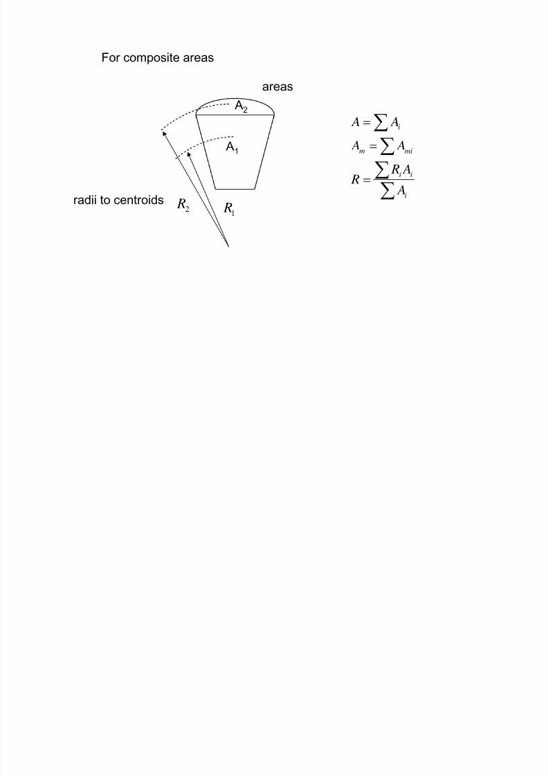
For composite areas

A1

A2

1 R2

R

i

m mi

i i

i

A A

A A

R A R

A

=

=

=

∑

∑∑∑

radii to centroids

areas



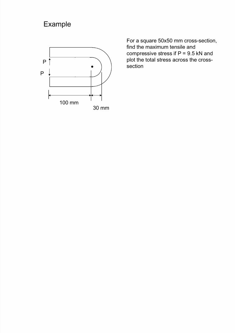
Example

P

P

100 mm30 mm

For a square 50x50 mm cross-section,

find the maximum tensile and

compressive stress if P = 9.5 kN and

plot the total stress across the cross-

section



P = 9500 N

M

N

155 mm

a

c

b

( )

2

lnm

A b c a

a c R

c A b

a

= −

+=

⎛ ⎞= ⎜ ⎟⎝ ⎠

a = 30 mm

b = 50 mm

c = 80 mm

so we have

( ) ( ) 250 50 2500

8050ln 49.04

30

80 30 552

m

A mm

A mm

R mm

= =

⎛ ⎞= =⎜ ⎟⎝ ⎠

+= =

250051

49.04n R mm= =

T C



max tensile stress is at r = 30 mm

( )

( )

( ) ( ) ( ) ( )( )( ) ( )( )155 9500 2500 30 49.049500

2500 2500 30 55 49.04 2500

106.2

m

m

M A rA N

A Ar RA A

MPa

θθ σ

−= +

−

−⎡ ⎤⎣ ⎦= +−⎡ ⎤⎣ ⎦

=

max compressive stress is at r = 80 mm

( )

( )( ) ( ) ( ) ( )

( ) ( ) ( ) ( )

155 9500 2500 80 49.049500

2500 2500 80 55 49.04 2500

49.3

m

m

M A rA N

A Ar RA A

MPa

θθ σ −

= +

−−⎡ ⎤⎣ ⎦= +

−⎡ ⎤⎣ ⎦= −



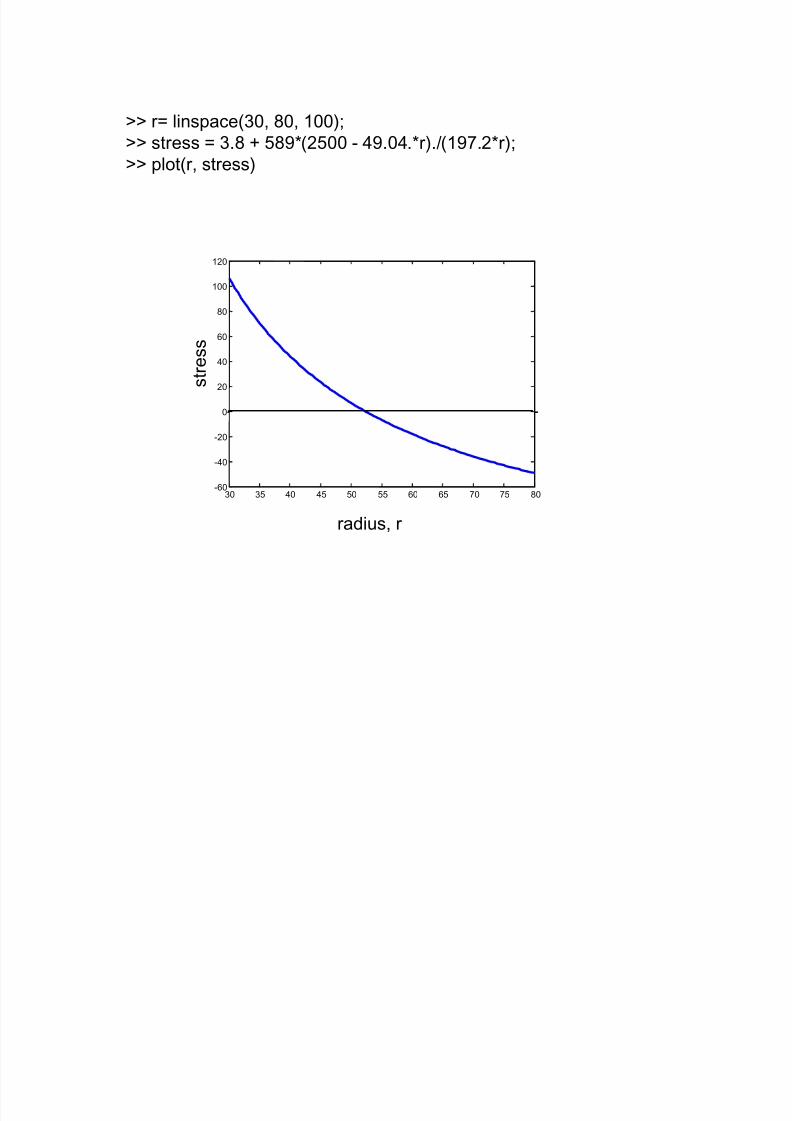
>> r= linspace(30, 80, 100);

>> stress = 3.8 + 589*(2500 - 49.04.*r)./(197.2*r);

>> plot(r, stress)

30 35 40 45 50 55 60 65 70 75 80-60

-40

-20

0

20

40

60

80

100

120

radius, r

s t r e s s



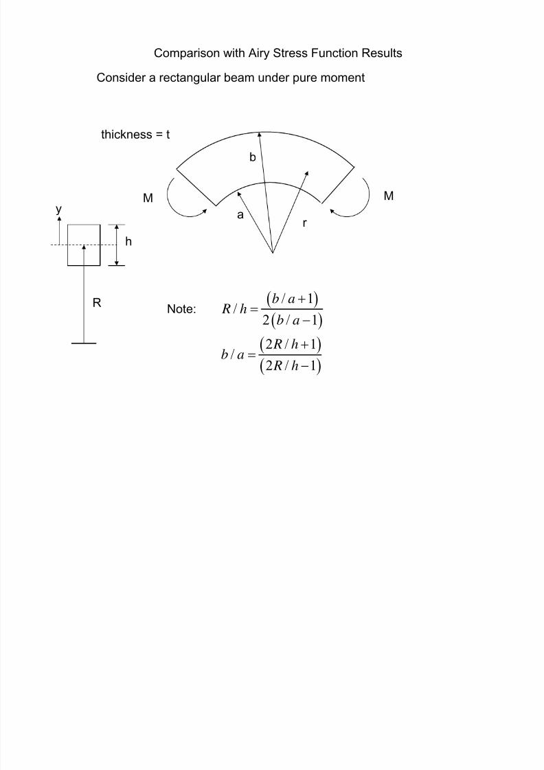
Comparison with Airy Stress Function Results

Consider a rectangular beam under pure moment

a

b

r

MM

thickness = t

R

h

Note: ( )( )

( )

( )

/ 1/

2 / 1

2 / 1/

2 / 1

b a R h

b a

R hb a

R h

+=−

+=

−

y



2 2 2

2

4ln ln ln 1

M a b b b r a r b

Nta r a a a a b a a

θθ σ ⎡ ⎤⎛ ⎞ ⎛ ⎞ ⎛ ⎞ ⎛ ⎞ ⎛ ⎞ ⎛ ⎞= − + − + −⎢ ⎥⎜ ⎟ ⎜ ⎟ ⎜ ⎟ ⎜ ⎟ ⎜ ⎟ ⎜ ⎟

⎝ ⎠ ⎝ ⎠ ⎝ ⎠ ⎝ ⎠ ⎝ ⎠ ⎝ ⎠⎢ ⎥⎣ ⎦

From Airy Stress Function

2 22 2

1 4 lnb b b

N a a a

⎡ ⎤ ⎡ ⎤⎛ ⎞ ⎛ ⎞ ⎛ ⎞= − −⎢ ⎥⎜ ⎟ ⎜ ⎟ ⎜ ⎟⎢ ⎥⎝ ⎠ ⎝ ⎠ ⎝ ⎠⎣ ⎦⎢ ⎥⎣ ⎦

Strength Approach

( )

( )

ln

/ 2

m

b A t

a

A t b a

R a b

⎛ ⎞= ⎜ ⎟⎝ ⎠

= −

= +



( )

( )( )

( ) ( )

( )

2

ln

ln

2

2 1 ln

1 2 1 1 ln

m

m

M A rA

Ar RA Ab

M b a r a

a b bt r b a b a

a

b r b M

a a a

r b b b bt a

a a a a a

θθ σ − −

=

−⎡ ⎤⎛ ⎞− − − ⎜ ⎟⎢ ⎥⎝ ⎠⎣ ⎦=

+⎡ ⎤⎛ ⎞− − −⎜ ⎟⎢ ⎥⎝ ⎠⎣ ⎦

⎡ ⎤⎛ ⎞ ⎛ ⎞− −⎜ ⎟ ⎜ ⎟⎢ ⎥⎝ ⎠ ⎝ ⎠⎣ ⎦=⎡ ⎤⎛ ⎞⎛ ⎞ ⎛ ⎞ ⎛ ⎞ ⎛ ⎞− − − +

⎜ ⎟⎜ ⎟ ⎜ ⎟ ⎜ ⎟ ⎜ ⎟⎢ ⎥⎝ ⎠⎝ ⎠ ⎝ ⎠ ⎝ ⎠ ⎝ ⎠⎣ ⎦

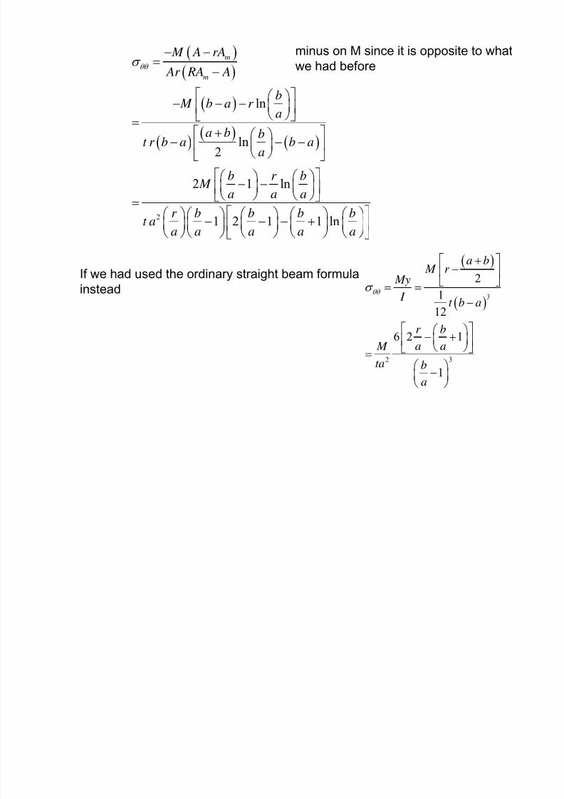
If we had used the ordinary straight beam formula

instead

( )

( )

3

32

2

1

12

6 2 1

1

a b M r

My

I

t b a

r b

a a M

ta b

a

θθ σ

+⎡ ⎤−⎢ ⎥

⎣ ⎦= =

−⎡ ⎤⎛ ⎞− +⎜ ⎟⎢ ⎥⎝ ⎠⎣ ⎦=

⎛ ⎞−⎜ ⎟⎝ ⎠

minus on M since it is opposite to what

we had before



Comparison of the ratio of the max bending stresses

0.93310.99945.0

0.88810.99863.0

0.83130.99732.0

0.77370.99611.5

0.65450.99701.0

0.52621.01240.75

0.43901.04550.65

Strength/elasticity

Straight beam

formula My/I

Strength/elasticity

Curved beam

formula

R/h

R

h

y



Compare bending stress distributions at the smallest R/h value

1 2 3 4 5 6 7 8-0.35

-0.3

-0.25

-0.2

-0.15

-0.1

-0.05

0

0.05

0.1

0.15

r/a

n o r m

a l i z e d s t r e s s

solid curve – Airy stress function (elasticity)

dashed blue – Curved Strength formula

dashed red – Straight beam formula

R/h = 0.65 (b/a = 7.667)



% beam_compare.m

m=1;

Rhvals = [0.65 0.75 1.0 1.5 2.0 3.0 5.0]; % R/h ratios to consider

for Rh = Rhvalsba = (1+2*Rh)/(2*Rh -1); %corresponding b/a values

ra= linspace(1, ba, 100); % r/a values

N=(ba^2-1)^2 -4*ba^2*(log(ba))^2;

% Airy function flexure stress expression

pa =4*(-(ba./ra).^2.*log(ba)+(ba)^2.*log(ra./ba) - log(ra) +(ba)^2 -1)./N;

% Curved beam strength expression for flexure stress

ps = 2*((ba-1)-ra.*log(ba))./(ra.*(ba-1).*(2.*(ba-1) -(ba+1).*log(ba)));% Straight beam flexure formula My/I

pb = 6*(2*ra-(ba+1))./((ba-1)^3);

%obtain ratio of max stresses Curved beam Strength formula/Airy

ratio1(m) = max(abs(ps))/max(abs(pa));

%obtain ratio of max stresses: Straight beam strength formula/Airy

ratio2(m) = max(abs(pb))/max(abs(pa));

m=m+1;

end% Now plot stress distributions for smallest R/h value

Rh=0.65

ba = (1+2*Rh)/(2*Rh -1); %corresponding b/a values

ra= linspace(1, ba, 100);

N=(ba^2-1)^2 -4*ba^2*(log(ba))^2;

pa =4*(-(ba./ra).^2.*log(ba)+(ba)^2.*log(ra./ba) - log(ra) +(ba)^2 -1)./N;

ps = 2*((ba-1)-ra.*log(ba))./(ra.*(ba-1).*(2.*(ba-1) -(ba+1).*log(ba)));pb = 6*(2*ra-(ba+1))./((ba-1)^3);

plot(ra, pa)

hold on

plot(ra, ps, '--b')

plot(ra, pb, '--r')

xlabel('r/a')

ylabel( 'normalized stress')

hold off



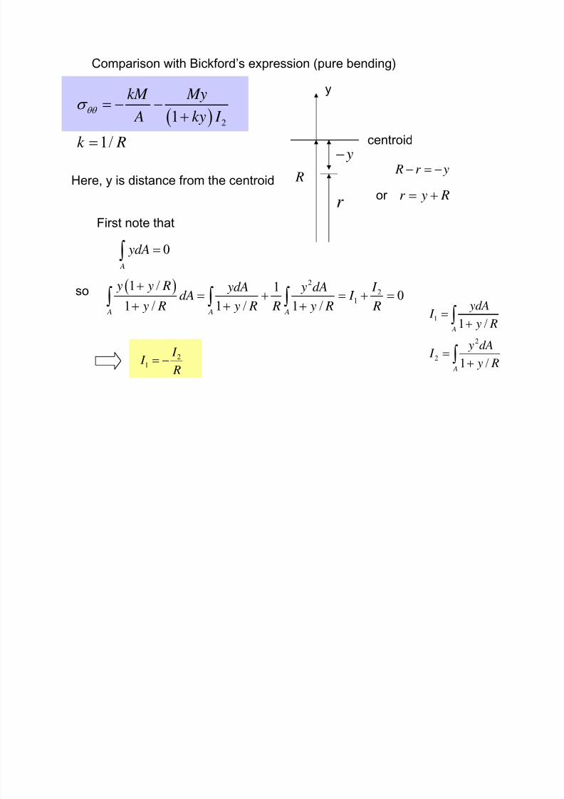
Comparison with Bickford’s expression (pure bending)

( ) 21

1/

kM My

A ky I

k R

θθ σ = − −+

=

R

r

centroid

y

y−

First note that

0

A

ydA =∫

Here, y is distance from the centroid

so ( ) 2

2

1

1 / 10

1 / 1 / 1 / A A A

y y R I ydA y dAdA I

y R y R R y R R

+= + = + =

+ + +∫ ∫ ∫ 1

2

2

1 /

1 /

A

A

ydA I y R

y dA I

y R

=+

=+

∫

∫2

1

I I

R= −

R r y− = −

or r y R= +



m A A

dA dA RA R R

r y R= =

+∫ ∫( )

( )

1

A A A A

m

y R y dA A dA dA dA R

y R y R y R

I RA R

+= = = +

+ + +

= +

∫ ∫ ∫ ∫

1 / I R

Thus,( ) 1 2

/m R RA A I I R− = − =



( ) 21

1/

kM My

A ky I

k R

θθ σ = − −+

=

Now, start with Bickford’s expression

( )

( )

( )

( ) ( )

( ) ( )

( )

( )

( ) ( )

( )

2

2

2

2

2 32

2 2

2 2

2

2 2

222

2 2

2 3

2

2

2

1

/

/

yR M

AR y R I

y R I yAR M

y R ARI

y R I y R AR AR

M y R ARI y R ARI

I AR R M

ARI y R I

I AR R M

y R I ARI

A y R I AR R M

y R AI R

θθ σ ⎡ ⎤

= − +⎢ ⎥+⎣ ⎦

⎡ ⎤+ += − ⎢ ⎥

+⎣ ⎦

⎡ ⎤+ + +

= − −⎢ ⎥+ +⎣ ⎦

⎡ ⎤+= − −⎢ ⎥

+⎣ ⎦

⎡ ⎤+= −⎢ ⎥+⎣ ⎦

⎡ ⎤− + +⎢ ⎥=

+⎢ ⎥⎣ ⎦

same terms added in and subtracted out



( ) ( )( )

2 3

2

2

2

/

/

A y R I AR R

M y R AI Rθθ σ

⎡ ⎤− + +

⎢ ⎥= +⎢ ⎥⎣ ⎦

but 2

2 /m RA A I R− = so ( )2 3

2 /m A I AR R= +

and we find

y R r + =

( )m

m

A rA

r RA A Aθθ σ

⎡ ⎤−= ⎢ ⎥

−⎣ ⎦

which agrees with our previous expression



from Bickford’s expression

( ) 21

1/

kM My

A ky I

k R

θθ σ = − −+

=

it is easy to see, as , R → ∞ 0k →

and 2

2

2

1 / A A

y dA I y dA I

y R

= → =

+∫ ∫

and we recover the straight beam flexure expression

My

I θθ σ = −

winkler curved beam theory

Documents