wind tunnel based anemometer testing facility
TRANSCRIPT

i
Wind Tunnel Based Anemometer Testing Facility
By
BENSON LUTHER GILBERT B.S. (University of California, Davis) 2006
THESIS
Submitted in partial satisfaction of the requirements for the degree of
MASTER OF SCIENCE
in
MECHANICAL AND AERONAUTICAL ENGINEERING
in the
OFFICE OF GRADUATE STUDIES
of the
UNIVERSITY OF CALIFORNIA
DAVIS
Approved:
______________________________________ C.P. van Dam, Chair
______________________________________
Bruce R. White
______________________________________ Paul Erickson
Committee in Charge
2010

UMI Number: 1489374
All rights reserved
INFORMATION TO ALL USERS The quality of this reproduction is dependent upon the quality of the copy submitted.
In the unlikely event that the author did not send a complete manuscript
and there are missing pages, these will be noted. Also, if material had to be removed, a note will indicate the deletion.
UMI 1489374
Copyright 2011 by ProQuest LLC. All rights reserved. This edition of the work is protected against
unauthorized copying under Title 17, United States Code.
ProQuest LLC 789 East Eisenhower Parkway
P.O. Box 1346 Ann Arbor, MI 48106-1346

ii
ABSTRACT
Measured estimates of the wind resource available at a site are performed with the use of
an anemometer. The accuracy of the wind measurements is vital to determining the wind
resource of wind farms, which is why great care must be taken in calibrating
anemometers. The purpose of this project was to prepare the University of California,
Davis (UCD) Aeronautical Wind Tunnel (AWT) for automatically calibrating
anemometers with the use of a virtual instrument (VI) created in LabVIEW that measures
the wind tunnel and anemometer quantities and controls the wind tunnel speed. The
initial calibration was conducted using an RM Young propeller type anemometer that has
been benchmarked by National Institute of Standards and Technology (NIST) and is used
by the industry to compare anemometer calibration facilities. A second verification of
the wind tunnel’s readiness to calibrate anemometers was performed using a pitot-static
probe manufactured by United Senor Corporation.

iii
To my wife, Jennifer, for always being my life, love and inspiration!

iv
ACKNOWLEDGEMENTS
I would like to thank OTECH Engineering Inc., particularly Rachael Coquilla and John
Obermeier, for their assistance with calibration and their advisement on anemometer
calibration.
I cannot leave out Mike Akahori and Sean Malone at the University of California (UC),
Davis machine shop for assisting me with machining the parts I needed for the wind
tunnel. Thank you, Ray Chow, for helping me with computer problems that cropped up
during my research, and for helping to reformat the wind tunnel computer. I’d like to
thank Henry Shiu for his advice and direction on this thesis. Jon Baker was a key partner
in my research, as it was he that taught me the ropes at the wind tunnel, instructed me in
LabVIEW and provided guidance along each step of the way.
A big thank you is definitely in order for Professor C.P. “Case” van Dam, for his overall
direction on my thesis, for his support and assistance along every step of this research.
Thank you to Professor Bruce White and Professor Paul Erickson for reviewing my thesis
and offering your suggestions.
I would like to thank my family for their continual support during my education. They
have put up with me being tardy, preoccupied and unavailable as I plowed through UC
Davis in pursuit of my Masters. Thank you for your patience with me and your
understanding during this busy and trying time. I’m finally free now, which means that I

v
can finally get around to fixing those watches, upgrading your computers and helping you
with all those projects that I’ve been promising to get to for years.
I would like to thank my mom, Linda, for her support and assistance with my high school
science fair projects. Without her support and encouragement, I might not have pursed
aeronautics past those small-scale projects.
Thank you, Dad, for teaching me persistence and determination and for bringing me up to
be comfortable working around tools and machinery. Those skills have not only proved
valuable in completing my research, but in my career as well.
Above all I would like to thank my wife who has supported me every inch of the way in
performing my research and completing this thesis. She has been and continues to be my
inspiration and sanity! Without her there is no doubt that I would have lost my mind in
pursuit of completing this thesis.

vi
TABLE OF CONTENTS
ABSTRACT ........................................................................................................................ ii
ACKNOWLEDGEMENTS ............................................................................................... iv
TABLE OF CONTENTS ................................................................................................... vi
LIST OF TABLES ............................................................................................................ xii
LIST OF FIGURES ......................................................................................................... xiii
NOMENCLATURE ..........................................................................................................xv
1. INTRODUCTION ......................................................................................................1
1.1: BACKGROUND .................................................................................................1
1.2: PROJECT OVERVIEW ....................................................................................4
2. UCD AWT FACILITY WITH UPGRADES FOR ANEMOMETER CALIBRATION .........................................................................................................8
2.1: WIND TUNNEL ......................................................................................................8
2.1.1: Contraction Section ..................................................................................9
2.1.2: Test Section .............................................................................................10
2.1.3: Top of Test Section/Plenum ...................................................................11
2.1.4: Diffusion Section .....................................................................................11
2.1.5: Wind Tunnel Fan ...................................................................................12
2.2: DATA ACQUISITION AND MEASUREMENT SYSTEM ........................12
2.2.1: Wind Tunnel Computer ........................................................................12
2.2.2: NI SCB-100 DAQ Box ............................................................................13
2.2.3: Pressure Taps and Differential Pressure Transducers .......................13
2.2.4: TRH Transmitter ...................................................................................15
2.2.5: Transducer #5 .........................................................................................17

vii
2.2.6: RM Young Anemometer ........................................................................18
2.2.7: Pitot-Static Probe and Traversing Mechanism ...................................19
3. CALIBRATION METHOD ....................................................................................19
3.1: CALIBRATION REQUIREMENTS .............................................................19
3.2: CALIBRATION PROGRAM .........................................................................23
3.2.1: Functional Block Diagram ....................................................................23
3.2.1.1: Inputs ..............................................................................................24
3.2.1.2: Outputs (Data) ...............................................................................24
3.2.1.3: Outputs (Results) ............................................................................25
3.2.2: Computer Running LabVIEW 8.5 VI ..................................................25
3.3: CALIBRATION PROCEDURE .....................................................................30
3.3.1: Anemometer or Pitot-Static Probe Setup ............................................30
3.3.2: Automated Fan Control Manual Test Voltages ..................................33
3.3.3: Run Calibration Test .............................................................................34
3.4: UNCERTAINTY ANALYSIS .........................................................................36
3.4.1: Reason for Uncertainty Analysis ..........................................................37
3.4.2: Uncertainty Analysis Background ........................................................37
3.4.3: Bias Error ...............................................................................................38
3.4.3.1: Calibration Errors .........................................................................40
3.4.3.2: Digitizing Error .............................................................................41
3.4.3.3: DAQ Error .....................................................................................42
3.4.3.4: Data Reduction Error ....................................................................42
3.4.3.5: Installation Error ...........................................................................43
3.4.3.6: Conceptual Errors .........................................................................44
3.4.4: Precision Error .......................................................................................45

viii
3.4.5: Uncertainty Analysis for the Anemometer ..........................................46
3.4.6: Uncertainty Analysis for the Wind Tunnel System ............................47
3.4.6.1: Absolute Sensitivity Coefficients (for Wind Tunnel System) ..........47
3.4.6.1.1: Absolute Sensitivity Coefficients for Uncalibrated Wind Tunnel Air Speed with Engineering Units ................51
3.4.6.1.2: Absolute Sensitivity Coefficients for Uncalibrated Wind Tunnel Air Speed with Voltage Units .......................52
3.4.6.2: Total Uncertainty Analysis for Wind Tunnel System .....................53
3.4.7: Uncertainty Analysis for the Pitot-Static Probe ..................................54
3.4.7.1: Absolute Sensitivity Coefficients for the Pitot-Static Probe ..........55
3.4.7.2: Total Uncertainty Analysis for the Pitot-Static Probe ...................57
3.4.8: Uncertainty Analysis Results ................................................................58
3.4.8.1: Wind Tunnel System .......................................................................58
3.4.8.2: Pitot-Static Probe: .........................................................................62
3.4.9: Uncertainty Analysis Discussion ...........................................................65
4. ANEMOMETER CALIBRATION RESULTS .....................................................68
4.1: REGULAR CALIBRATION TEST RESULTS ............................................68
4.2: HYSTERESIS CALIBRATION TEST RESULTS .......................................81
5. DISCUSSION ............................................................................................................82
6. CONCLUSIONS AND RECOMMENDATIONS .................................................90
7. REFERENCES .........................................................................................................91
8. APPENDIX A: CALIBRATED RM YOUNG PROPELLER ANEMOMETER ......................................................................................................95
Figure A-1: NIST Traceable anemometer calibration certificate provided by OTECH Engineering Incorporated[20]. .................................................95
Figure A-2: User’s manual for the RM Young anemometer (Model Number 27106DR), page 1 of 5[21]. ...................................................................96

ix
Figure A-3: User’s manual for the RM Young anemometer (Model Number 27106DR), page 2 of 5[21]. ...................................................................97
Figure A-4: User’s manual for the RM Young anemometer (Model Number 27106DR), page 3 of 5[21]. ...................................................................98
Figure A-5: User’s manual for the RM Young anemometer (Model Number 27106DR), page 4 of 5[21]. ...................................................................99
Figure A-6: User’s manual for the RM Young anemometer (Model Number 27106DR), page 5 of 5[21]. .................................................................100
9. APPENDIX B: PITOT-STATIC PROBE ...........................................................101
Figure B-1: Original dimensioned drawing of the pitot-static probe[22]. ...............101
10. APPENDIX C: WIND TUNNEL INSTRUMENT SPECIFICATIONS ..........102
Table C-1: Current setup of all data cables wired to the SCB-100 connector box. ....................................................................................102
Figure C-1: Current setup notes regarding all data cables wired to the SCB-100 connector box. .............................................................................103
Figure C-2: Calibration details for Transducer #1[37]. ...........................................104
Figure C-3: Calibration details for Transducer #2[29]. ...........................................105
Figure C-4: Calibration details for Transducer #4[38]. ...........................................106
Figure C-5: Calibration details for the Temperature Transmitter[39]. ....................107
Figure C-6: Calibration details for the Relative Humidity Transmitter[39]. ...........108
Figure C-7: Calibration details for Transducer #5[40]. ...........................................109
11. APPENDIX D: WIND TUNNEL BOUNDARY-LAYER ANALYSIS .............110
Figure D-1: Boundary-layer thickness graph for laminar flow in the UCD AWT test section using the flat plate assumption. .............................110
Table D-1: Boundary-layer thickness calculations for laminar flow in the AWT test section using the flat plate assumption[26]. ........................111
Figure D-2: Boundary-layer thickness graph for turbulent flow in the UCD AWT test section using the flat plate assumption. .............................112

x
Table D-2: Boundary-layer thickness calculations for turbulent flow in the AWT test section using the flat plate assumption[26]. ........................113
12. APPENDIX E: ANEMOMETER SUPPORT STRUCTURE ...........................114
Figure E-1: Bridgeport three and a half axis milling machine set up to machine the slot cover for the anemometer leveling support structure (left). Close up of the slot cover partially completed on the milling machine (right). ..........................................................114
Figure E-2: Exploded view of the “L” shaped pipe assembly (also known as the support pipe) that is composed of a 3/4 in. diameter schedule 40 galvanized steel pipe, elbow fitting, extension fitting and an anemometer female 4-pin (7 hole) connector, all of which is used in the anemometer leveling support structure. ........114
Figure E-3: Top view of the following anemometer leveling support structure components that are responsible for leveling the anemometer: the pipe clamp (top left), leveling plate (top center), base plate (top right), and slot cover (bottom). .....................115
Figure E-4: Top view of the pipe clamp (top left), leveling plate (top center), and the base plate (top right). Bottom view of the slot cover (bottom). ...................................................................................115
Figure E-5: Top close-up view of the pipe clamp (top left). Note that the slot on the pipe clamp (located at the bottom is this picture) will point in the direction of the air flow in the UCD AWT test section when the anemometer leveling support structure is properly installed. ..............................................................................116
Figure E-6: The fully assembled support pipe (top), and the fully assembled leveling structure (bottom) that when combined make up the anemometer leveling support structure. .............................................116
Figure E-7: Bottom view of the anemometer leveling support structure, minus the support pipe, shown as properly installed in a slot. ..........117
Figure E-8: Top left view of the anemometer leveling support structure installed in a slot on the roof of the UCD AWT test section. ............117
Figure E-9: Top view of the anemometer leveling support structure installed in a slot on the roof of the UCD AWT test section. ............118

xi
Figure E-10: Top close-up view focused on the base plate, leveling plate, pipe clamp, and support pipe when the anemometer leveling support structure is installed in a slot on the roof of the UCD AWT test section................................................................................118
Figure E-11: Top close-up view (left) and top right close-up view (right) focused on the leveling plate, pipe clamp, and support pipe when the anemometer leveling support structure is installed in a slot on the roof of the UCD AWT test section. ...............................119
Figure E-12: Top left close-up view (left) and top close-up view (right) focused on the leveling plate, pipe clamp, and support pipe when the anemometer leveling support structure is installed in a slot on the roof of the UCD AWT test section. ...............................119
Figure E-13: Left side view of the anemometer leveling support structure installed in a slot on the roof of the UCD AWT test section, without an anemometer installed on the support pipe. ......................120
13. APPENDIX F: ANEMOMETER CALIBRATION PROGRAM .....................121
Figure F-1: Front panel of the calibration program, showing the “Real Time Data and Results” tab which displays all data and results used in anemometer calibration. ........................................................121
Figure F-2: Front panel of the calibration program, showing the “Fan Control” tab with the “Manual Fan Control” sub-tab which together display all the inputs and outputs required to successfully operate the wind tunnel fan manually. ..........................122
Figure F-3: Front panel of the calibration program, showing the “Fan Control” tab with the “Automated Fan Control” sub-tab which together display all the inputs and outputs required to successfully operate the wind tunnel fan automatically. Note that the wind tunnel fan was operated automatically for both the anemometer and pitot-static tests. ................................................123

xii
LIST OF TABLES
Table 3.4.3-1: Bias error values for the following measured variables used in the anemometer and pitot-static probe calibration tests: barometric pressure, temperature and relative humidity[25, 27, 28]. ..........39
Table 3.4.3-2: Bias error values for the following measured variables used in the anemometer and pitot-static probe calibration tests: differential pressure T1 (∆PT1) and differential pressure T3 (∆PT3)[23, 25]. ...........................................................................................40
Table 3.4.4-1: Minimum and maximum precision error limit values for each measured variable in both the anemometer and pitot-static probe calibration tests (for the desired air speed range of 4 to 26 m/s). ..........46
Table 3.4.8.1-1: Uncertainty results of the middle position anemometer calibration tests for uncalibrated wind tunnel air speed. .......................59
Table 3.4.8.1-2: Uncertainty results of the middle position anemometer calibration tests for calibrated wind tunnel air speed. ...........................61
Table 3.4.8.2-1: Uncertainty results of the middle position pitot-static probe calibration tests for corrected pitot-static air speed. ..............................64
Table 4.1-1: Anemometer position location compared with anemometer calibration coefficients (slope and intercept) obtained from the wind tunnel linear calibration equations in Figures 4.1-1 to 4.1-3, (where VREF = MVUC + I, is the general equation form). ..................72
Table 4.1-2: Pitot-Static probe position location compared with pitot-static probe calibration coefficients (slope and intercept) obtained from the wind tunnel linear calibration equations in Figures 4.1-1 to 4.1-3. ...............................................................................................73
xiii
LIST OF FIGURES
Figure 1.1-1: Sketch of a cup anemometer[14]. .............................................................3
Figure 1.1-2: Picture of a windmill anemometer (left)[17] and three propeller anemometers setup to measure the three velocity components of wind (right)[18]. ...................................................................................4
Figure 1.2-1: RM Young propeller anemometer installed in the UCD AWT at the front position. ...............................................................................7
Figure 1.2-2: United Senor Corporation pitot-static probe installed in the UCD AWT at the front position.............................................................8
Figure 2.1-1: UCD AWT System Diagram .................................................................9
Figure 3.2.2-1: VI Functional Block Diagram for the calibration program .................27
Figure 3.4.6.1-1: Illustration of how the wind tunnel calibration slope, M, and intercept, I, coefficients were determined and the calibrated air speed equation formed. ........................................................................49
Figure 3.4.8.1-1: Uncertainty results of the middle position anemometer calibration tests for uncalibrated wind tunnel air speed and calibrated wind tunnel air speed. .........................................................62
Figure 3.4.8.2-1: Uncertainty results of the middle position pitot-static probe calibration tests for corrected pitot-static air speed. ............................65
Figure 4.1-1: Anemometer and pitot-static probe measurements versus uncalibrated wind tunnel air speed in the front of the wind tunnel test section. ................................................................................69
Figure 4.1-2: Anemometer and pitot-static probe measurements versus uncalibrated wind tunnel air speed in the middle of the wind tunnel test section. ................................................................................70
Figure 4.1-3: Anemometer and pitot-static probe measurements versus uncalibrated wind tunnel air speed in the back of the wind tunnel test section. ................................................................................71
xiv
Figure 4.1-4: Anemometer and pitot-static probe linear calibration equation slopes for the front, middle and back wind tunnel test section positions. ..............................................................................................74
Figure 4.1-5: Anemometer and pitot-static probe linear calibration equation intercepts for the front, middle and back wind tunnel test section positions. ..................................................................................75
Figure 4.1-6: Anemometer and pitot-static probe measurements versus calibrated wind tunnel air speed in the front of the wind tunnel test section. ...........................................................................................76
Figure 4.1-7: Anemometer and pitot-static probe measurements versus calibrated wind tunnel air speed in the middle of the wind tunnel test section. ................................................................................77
Figure 4.1-8: Anemometer and pitot-static probe measurements versus calibrated wind tunnel air speed in the back of the wind-tunnel test section. ...........................................................................................78
Figure 4.1-9: Uncalibrated and calibrated wind tunnel air speed versus anemometer frequency for tests in the front of the wind-tunnel test section (with the OTECH Engineering calibration curve displayed for comparison)....................................................................79
Figure 4.1-10: Uncalibrated and calibrated wind tunnel air speed versus anemometer frequency for tests in the middle of the wind tunnel test section (with the OTECH Engineering calibration curve displayed for comparison). .........................................................80
Figure 4.1-11: Uncalibrated and calibrated wind tunnel air speed versus anemometer frequency for tests in the back of the wind tunnel test section (with the OTECH Engineering calibration curve displayed for comparison)....................................................................81
xv
NOMENCLATURE
Term/Acronym Definition
° Degree (unit of measure for angles)
% RH Percent relative humidity
A or amp Ampere (unit of electrical current)
ASTM American Society for Testing and Materials
AWT Aeronautical Wind Tunnel
DAQ Data acquisition
Frac % Fractional percent [range 0 to 1, unitless] unit used for relative humidity values
FSR or FS Full scale range, usually in reference to the output voltage range of an instrument. This is also known as full scale (FS).
GB Gigabyte (quantity unit for RAM or hard drive capacity)
IEC International Electrotechnical Commission
INWC Inches of water, is a unit of pressure
I/O Input or output communication channels in a computer system
LabVIEW National Instruments program that utilizes a graphic oriented programming language
NI National Instruments
NIST National Institute of Standards and Technology
NRG #40 Common cup anemometer made by NRG Systems
PID Proportional-integral-derivative (such as a PID controller)
R Correlation coefficient
R2 Coefficient of determination
RAM Random-access memory
RC Resistor capacitor (such as an RC Filter)
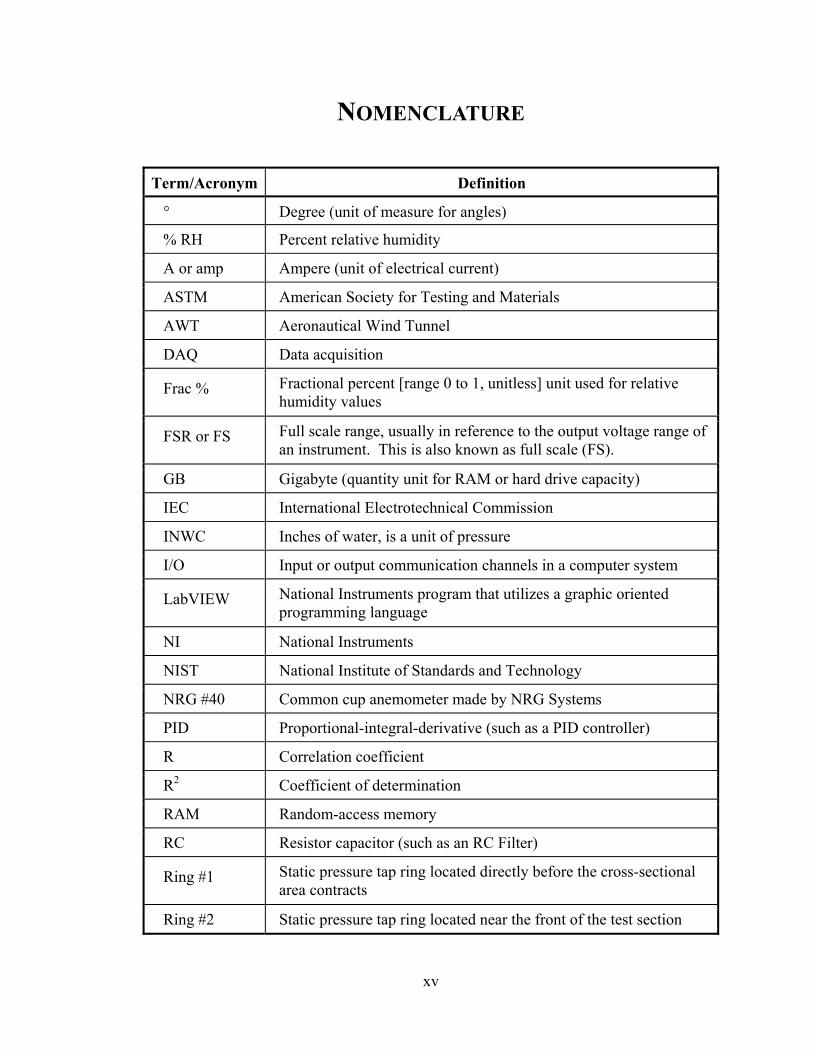
Ring #1 Static pressure tap ring located directly before the cross-sectional area contracts
Ring #2 Static pressure tap ring located near the front of the test section
xvi
Term/Acronym Definition
RSS Root-sum-square method
SI International System of Units
S/s Samples per second (unit of measure for data acquisition card speed)
subVI A virtual instrument program embedded within a virtual instrument program
T1 Differential pressure transducer #1 (Transducer #1)
T2 Differential pressure transducer #4 (Transducer #4)
T3 Differential pressure transducer #2 (Transducer #2)
TRH Temperature/relative humidity
UC University of California
UCD University of California, Davis
V Volt (unit of electrical voltage)
VDC Direct current voltage
VI Virtual instrument program
Symbol Definition Constant Value
Units Source
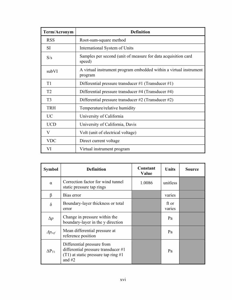
α Correction factor for wind tunnel static pressure tap rings
1.0086 unitless
β Bias error varies
δ Boundary-layer thickness or total error
ft or varies
∆p Change in pressure within the boundary-layer in the y direction
Pa
∆pref Mean differential pressure at reference position
Pa
∆PT1 Differential pressure from differential pressure transducer #1 (T1) at static pressure tap ring #1 and #2
Pa

xvii
Symbol Definition Constant Value
Units Source
∆PT3
Differential pressure from differential pressure transducer #2 (T3) that measures the pressure difference between the total pressure port and the static pressure ports on the pitot-static probe
Pa
∆y Distance from the wall to the edge of the boundary-layer
m
ε Precision error varies
µ Dynamic viscosity for air Pa·s
µo Reference dynamic viscosity for air at reference absolute temperature
1.716×10⁻⁵ Pa·s [1]
ρ Air density kg/m3
φ Relative humidity Frac %
b Bits or bit b
B Barometric pressure Pa
BE Bias error limit varies
b∆PT1 Differential pressure calibration equation intercept constant
1.0066 Pa
b∆PT3 Differential pressure calibration equation intercept constant
6.7976×10⁻² Pa
bφ Relative humidity calibration equation intercept constant
6.48×10⁻³ Frac %
bB Barometric pressure calibration equation intercept constant
80001.740 Pa
( )DiB Digitizing bias error varies
bT Absolute temperature calibration equation intercept constant
264 K
c1 Constant in vapour pressure equation
0.0000205 unitless [2]

xviii
Symbol Definition Constant Value
Units Source
c2 Constant in vapour pressure equation
0.0631846 unitless [2]
Ch Pitot tube head coefficient for a Reynolds number greater than 2000
1 unitless [3]
i Given instrument
I Wind tunnel calibration intercept coefficient for the front, middle or back test section position
m/s
j Individual measurement or sample unitless
kb Blockage correction factor 1 unitless
kc Wind tunnel calibration factor 1 unitless
ℓ Characteristic length ft
M Wind tunnel calibration slope coefficient for the front, middle or back test section position
unitless
m∆PT1 Differential pressure calibration equation slope constant
746.92 Pa/V
m∆PT3 Differential pressure calibration equation slope constant
124.53 Pa/V
mφ Relative humidity calibration equation slope constant
0.959 1/V
mB Barometric pressure calibration equation slope constant
5998.7640 Pa/V
mT Absolute temperature calibration equation slope constant
1.50×10² K/V
n Number of samples per interval 1 unitless
N Number of samples in the sample population
27000 unitless
O Boundary-layer’s order of magnitude
unitless
PE Precision error limit varies

xix
Symbol Definition Constant Value
Units Source
Pw Vapor pressure Pa
Re Reynolds number for the pitot-static probe
unitless
Ro Specific gas constant of dry air 287.0553 J/kg·K [4, 5, 6]
Rw Specific gas constant of water vapor 461.5232 J/kg·K [4, 5, 6]
S Sutherland's constant for air 110.4 K [7, 8]
SEE Standard error varies
SX Standard deviation for the data population
varies
t Value for the t-distribution at a confidence level of 95%
1.9601 unitless
T Absolute temperature of air in the test section
K
To Reference absolute temperature 273.15 K [5]
U Total uncertainty varies
U∆PT1 Total differential pressure
uncertainty for differential pressure transducer #1 (T1)
Pa
U∆PT3 Total differential pressure
uncertainty for differential pressure transducer #2 (T3)
Pa
Uφ Total relative humidity uncertainty Frac %
UB Total barometric pressure uncertainty
Pa
UT Total absolute temperature uncertainty
K
UV∆PT1 Total differential pressure uncertainty for differential pressure transducer #1 (T1)
V

xx
Symbol Definition Constant Value
Units Source
UV∆PT3 Total differential pressure voltage output uncertainty for differential pressure transducer #2 (T3)
V
UVφ Total relative humidity voltage output uncertainty
V
UVB Total barometric pressure voltage output uncertainty
V
UVC Total calibrated wind tunnel air speed uncertainty
m/s
UVCPS Total corrected pitot-static air speed uncertainty
m/s
UVT Total absolute temperature voltage output uncertainty
V
UVUC Total uncalibrated wind tunnel air speed uncertainty
m/s
Ux Total uncertainty for a measured variable
varies
v Mean air speed m/s
Var Variance = SX2 varies
V∆PT1 Differential pressure voltage output from differential pressure transducer #1 (T1) at static pressure tap ring #1 and #2
V
V∆PT3
Differential pressure voltage output from differential pressure transducer #2 (T3) that measures the pressure difference between the total pressure port and the static pressure ports on the pitot-static probe
V
Vφ Relative humidity voltage output V
VB Barometric pressure voltage output V
VC Calibrated wind tunnel air speed m/s

xxi
Symbol Definition Constant Value
Units Source
VCPS Corrected pitot-static air speed m/s
VREF Reference air speed (such as the calibrated air speed measured by the anemometer)
m/s
VT Absolute temperature voltage output V
VUC Uncalibrated wind tunnel air speed m/s
xy Specific Cartesian plane
x Individual x value varies
x Average x value varies
X Measured variable
y Individual y value varies
y Average y value varies
Y Horizontal direction in the test section
Z Vertical direction in the test section
Units Systems: Throughout this thesis there are two main units of measurement systems: the International System of Units (SI) and the United States system of units (also known as English units). Since the wind tunnel and the parts that were manufactured for anemometer calibration were built to English units, all measurements regarding the wind tunnel and the manufacturing of parts were done using English units. However, with regards to both the ASTM (American Society for Testing and Materials) and IEC (International Electrotechnical Commission) anemometer calibration requirements and all other related measurements, the SI units were employed.

1
1. INTRODUCTION
1.1: BACKGROUND
In the wind energy industry, before a possible wind turbine farm site can be developed,
an estimate of the wind resource available at that site must be made in order to determine
if the site is a viable location for a wind energy farm. This estimate is based on
measurements conducted at the site using anemometers. Anemometers must be
accurately calibrated for determining the wind resource of a site; a measurement that is
off by as much as 1 m/s could mean a wind farm’s success or failure. Wind farm
economics are sensitive to the accuracy of the wind speed measurement because the
change in kinetic energy is proportional to the wind speed cubed. For example, if a wind
resource is measured at 11 m/s but is actually 10 m/s, this nominally 10% change in the
wind speed results in an approximately 33% drop in generated wind power[9]. This
example clearly demonstrates how crucial it is to accurately calibrate an anemometer.
The most commonly used anemometers today are the cup anemometer and the propeller
anemometer (or windmill type anemometer).
Thomas Romney Robinson was credited, in 1846, as the first to create a cup
anemometer[10], which is most praised for being the simplest instrument that measures
wind speed using the relationship between the rotational rate of the axis (that the cups
spin around) and the speed of the wind. Do to the simplicity of the cup anemometer and
its robust design; it has become one of the most widely used wind measurement devices
today. The NRG #40 is among the most universally used cup anemometers today[11],

2
which starts at about $160 (US dollars) and can go up to several hundred dollars
depending on the model and whether or not it is calibrated[12]. However, other more
complex cup anemometers can range up around $1500 depending upon its specific
functions[13].
An extensive review of the cup anemometer was recently presented by L. Kirstensen,
who points out that the cup anemometer possesses a near linear calibration curve, and
thus is able to achieve highly accurate wind speed measurements[14]. Kirstensen calls
attention to the work of C. E. Brazier, who discovered that the shorter the radius of the
arms that attach the cups to the axis, the more linear the calibration curve will be[14]. It is
for this reason that most cup anemometers have very short attachment arms, which in
turn help improve the accuracy of the calibration curve by making it more linear.
Cup anemometers are calibrated by relating known flow speeds to the rotational rate of
the axis. Unfortunately, because of the simplistic design, the cup anemometer is prone to
error in measuring the average wind speed in the horizontal plane (the xy plane when
referencing all three vector components of the wind in a Cartesian coordinate system).
This error shows up as a positive bias, or “overspeeding”, of the measured wind speed,
which is caused by the “asymmetric response to changes in wind speed”[14]. This means
that the air speed measurement by a cup anemometer will tend to be more accurate if the
air speed being observed is increasing rather than decreasing. It should be noted that all
anemometers should be calibrated at least once a year in order to ensure the accuracy of
the wind speed results[11]. A sketch of a cup anemometer is displayed in Figure 1.1-1.

3
Figure 1.1-1: Sketch of a cup anemometer[14].
Propeller anemometers are a type of windmill anemometer, with the exception that they
do not use wind vanes to force the propeller anemometer into the wind, but operate in a
fixed direction. Thus a plain propeller anemometer does not have the ability to measure
wind direction along with wind speed. The theory behind how windmill anemometers
operate is the same as the cup anemometers with the exception that the rotating axis is
horizontal instead of vertical and it is directly attached to the wind vane. The rotation of
the axis produces an alternating current sine wave with a frequency that is directly
proportional to the measured wind speed[15, 16]. Windmill anemometers are calibrated by
relating known flow speeds to the rotational rate of the axis, or the output frequency. The
advantage of the windmill anemometer is that it is able to determine both wind speed and
direction, unlike the cup anemometer. However, it does have the disadvantage of being
more expensive than the cup anemometer because it has two instruments instead of one
on the same device. A picture of both a windmill anemometer and a set of propeller
anemometers are displayed in Figure 1.1-2.

4
Figure 1.1-2: Picture of a windmill anemometer (left)[17] and three propeller anemometers setup to measure the three velocity components of wind (right)[18].
The anemometer used in this project is a propeller anemometer. The propeller
anemometer is very similar to a cup anemometer in both function and form, with the
exceptions that it operates on a horizontal axis instead of a vertical axis and it uses
propeller blades instead of cups to catch the air flow going past the anemometer. A
propeller anemometer is most sensitive to measuring wind parallel to its rotating axis,
whereas wind perpendicular to its axis of rotation is not measured at all[9]. The average
design accuracy for both the cup and propeller anemometer is approximately ± 2%[9].
1.2: PROJECT OVERVIEW
The purpose of this project is to upgrade and prepare the University of California, Davis
(UCD) Aeronautical Wind Tunnel (AWT) so that it can accurately perform calibration

5
tests for non-calibrated anemometers according to the requirements set forth in the
following two standards: “Standard Test Method for Determining the Performance of a
Cup Anemometer or Propeller Anemometer” (ASTM D 5096-02)[19] and in “Power
Performance Measurements of Electricity Producing Wind Turbines” (IEC 61400-12-
1)[2]. Anemometers are usually calibrated in a wind tunnel by relating a known wind
speed to the frequency produced by a given anemometer at the specific wind speed.
However, for this project, the first step was to prepare the UCD AWT for calibrating
anemometers. This was accomplished by installing the following additional instruments
to the tunnel: a temperature/relative humidity (TRH) transmitter, and a barometric
pressure transducer #5 (Transducer #5). These instruments coupled with the existing
pressure transducers make it possible to calculate the following using the inputs of the
instruments mentioned above: the air density, the wind tunnel air speed (in real time), and
the Reynolds number (in real time). These calculations were accomplished by creating a
virtual instrument program (VI) in LabVIEW. The VI was created with the ability to
manually input temperature, relative humidity and barometric pressure values in order to
test the program without the use of the aforementioned sensors and for troubleshooting
the program.
Once the VI was able to measure the wind speed in the tunnel in real time, a relationship
could be made between the wind speed of the wind tunnel and the voltage required by the
frequency controller of the wind tunnel’s fan. This relationship was used to automate the
calibration tests for anemometers by using the VI to control the frequency of the wind

6
tunnel fan. Hence, the wind speed of the tunnel could be controlled for specific durations
of time at specific wind speeds.
Once all of this was completed, an RM Young propeller anemometer (shown in Figure
1.2-1) that was benchmarked by OTECH Engineering to be NIST (National Institute of
Standards and Technology) traceable was tested in the UCD AWT in order to determine
the tunnel’s readiness to calibrate anemometers. This would be confirmed if the wind
tunnel is able to comply with the requirements of both of the following anemometer
calibration standards: the “Standard Test Method for Determining the Performance of a
Cup Anemometer or Propeller Anemometer” (ASTM D 5096-02)[19] or the “Power
Performance Measurements of Electricity Producing Wind Turbines” (IEC 61400-12-
1)[2]. The RM Young anemometer puts out a square wave signal that is directly related to
the wind speed that it measures. The frequency from this square wave and the NIST
traceable calibration curve is what is used by the VI to calculate the wind speed based on
the anemometer measurements. The NIST traceable calibration for the RM Young
anemometer was provided by OTECH Engineering. The calibration certificate[20]
provided by OTECH Engineering is shown in Figure A-1 in Appendix A. A copy of the
user’s manual for the RM Young anemometer (Model 27106DR)[21] is in Appendix A in
Figures A-2 to A-6.

7
Figure 1.2-1: RM Young propeller anemometer installed in the UCD AWT at the front position.
A second verification of the wind tunnel’s readiness to calibrate anemometers was
performed using a pitot-static probe (shown in Figure 1.2-2) manufactured by United
Senor Corporation (Model Number PDD-24-G-21-KL Straight). A copy of the original
dimensioned drawing of the pitot-static probe[22] is in Appendix B in Figure B-1. The
pressure differential of the total and static ports on the pitot-static probe were measured
by a differential pressure transducer manufactured by Setra Systems, Inc. with a range of
0 to 2.5 INWC (Model Number 239)[23].

8
Figure 1.2-2: United Senor Corporation pitot-static probe installed in the UCD AWT at the front position.
2. UCD AWT FACILITY WITH UPGRADES FOR ANEMOMETER CALIBRATION
2.1: WIND TUNNEL
The following information which describes the wind tunnel, its main sections and
components solely was based on information obtained from the UCD AWT Facility
website[24] and direct observations. The UCD AWT, which was installed in May 1997, is
primarily used for academic and research purposes. The UCD AWT is an open circuit
wind tunnel with an enclosed test section that is 33.6 in. by 48 in. and 12 ft. in length.
The UCD AWT is outfitted with a fan that is operated by a 125 horsepower motor that
produces a maximum velocity of approximately 165 mph (depending on the current air
density) through the test section. Turbulence levels in the test section have been
established to be less than or equal to 0.1% for the initial 80% of the test section

9
throughout the wind tunnel’s velocity range. The UCD AWT is composed of five main
sections: the contraction section, the test section, the plenum, the diffusion section, and
the wind tunnel fan. A simplified diagram of the UCD AWT is provided in Figure 2.1-1.
Figure 2.1-1: UCD AWT System Diagram
2.1.1: Contraction Section
The contraction section was designed to have a contraction ratio of 7.5 to 1; however, the
measured contraction ratio is actually 7.679 to 1. This contraction ratio was determined
by measuring the cross-sectional area of the contraction section both before and after
contraction, at the pressure taps for the two static pressure rings. These static pressure
tap rings are used to determine the air speed in the test section. The ring located directly
before the cross-sectional area contracts is designated as static pressure tap ring #1 (Ring
#1), and the ring located near the front of the test section is static pressure tap ring #2
(Ring #2). The measurements were performed with the use of a tape measure (with a
resolution of 1/16 in.), a height gauge (with a resolution of 0.001 in.), a pair of calipers

10
(with a resolution of 0.0005 in.) and a precision square that was used to help measure the
size of the fillets in the contraction section.
The flow straightener is located at the front of the contraction section. The first part of the
flow straightener is the trash screen, a coarse steel screen composed of 1 in. squares. The
second part is composed of an aluminum honeycomb filter that is 6 in. thick with 0.25 in.
cells. The cells have an aspect ratio of 24. The four anti-turbulence screens make up the
third part of the contraction section flow straightener. These 20 by 20 mesh screens
(0.009 in. diameter) are made of stainless steel. There is space for one more screen, if
ever needed.
The contraction chamber itself is composed of four identically curved sides that provide
equal pressure on each adjoining side. This helps to guard against the formation of corner
vortices.
2.1.2: Test Section
The test section of the wind tunnel contains two fairing turntables on the floor, each 36
in. in diameter. The front fairing table is synchronized with the pyramidal force balance
table to move to given angles of yaw. The back turntable moves independently in angles
of yaw. Instead of the usual diverging sides, the UCD AWT has parallel sides with four
tapered fillets to allow for boundary-layer growth and thus provide a constant static
pressure. The doors on the sides of the test section are made of Plexiglas and are
centered on the turntables. The doors are hinged at the top and can be removed and

11
replaced with glass if necessary. The ceiling and floor of the test section are made of
aluminum. For flow visualization, there is an 18 in. ultraviolet light (F18T8-BLB) on one
of the lower fillets centered on the front turntable. To provide a working light on the test
section, there are two 96 in. fluorescent lights (F96T8-SSCW) on the upper fillet panels.
2.1.3: Top of Test Section/Plenum
The Plenum contains the pyramidal force balance that is able to measure all six
components of force and moments (lift, drag, side force, pitching moment, rolling
moment and yawing moment) for an installed model. The force balance also moves the
model to a given angle of yaw (for two-dimensional models) and angle of attack (three-
dimensional models). On top of the test section there is a two dimension traversing
mechanism that can move a probe (such as the pitot-static probe used during this
research) horizontally and vertically within the cross-sectional plane of the test section.
2.1.4: Diffusion Section
The diffusion section is designed to slow down the airflow before crossing the path of the
fan. The diffusing section joins the test section to the fan. At the end of the diffuser,
there is a trash screen with 0.5 in. stainless steel mesh to protect the fan.
12
2.1.5: Wind Tunnel Fan
The wind tunnel fan is a Joy size 84-26-FB-1000 Arrangement 4 direct drive Axivane
vane-axial fan that has aluminum blades whose pitch can be manually adjusted. The fan
is run by a Reliance Electric premium efficient motor that operates on 3 phase, 460 V, 60
Hz power. The motor speed is controlled by a Mitsubishi Meltrac A-100 variable
frequency drive. The drive is designated MT-A140E-110K-02UL and is designed for 216
amp variable torque. The controller has a 1000:1 speed-ratio capability and can hold the
fan speed constant with a maximum variation of ±0.2%. The wind tunnel fan, which is
wired to the NI SCB-100 data acquisition (DAQ) box, is controlled by a subVI
(embedded virtual instrument) in the main VI that changes the voltage frequency and thus
the desired air speed that the wind tunnel fan produces. Downstream of the fan a sound
absorbing diffuser (silencer) was installed to suppress noise. To further reduce noise, the
central fan has a sound absorbent tail section.
2.2: DATA ACQUISITION AND MEASUREMENT SYSTEM
2.2.1: Wind Tunnel Computer
The DAQ computer has an AMD Athlon(tm) XP 2500+ processor, 1.00 GB of RAM at a
speed of 1.83 GHz, a partitioned hard drive that has the following two hard disk drives:
“Local Disk (C:)” with a total capacity of 29.9 GB and “Data (D:)” with a total capacity of
44.5 GB, and an Antec case. The computer’s operating system is Microsoft Windows XP
Professional Version 2002 with Service Pack 3. The computer is equipped with a PCI-
6071E DAQ card manufactured by National Instruments, which has the following

13
specifications: ±10 V range for analog input/output channels, 0 to 5 V range for digital
I/O and counter/timer channels, 1.25 MS/s for input channels, 1 MS/s for output
channels, 12-bit resolution for 64 single-ended analog input channels or 32 differential
input channels, 12-bit resolution for two analog output channels, eight digital I/O
channels and 24-bit resolution for two 20 MHz counter/timers[25]. The computer
currently has LabVIEW Professional Development System versions 6i, 8.2.1 and 8.5
installed.
2.2.2: NI SCB-100 DAQ Box
The NI SCB-100 DAQ connector box is used as the main hub for connecting the various
sensors and devices in the system to the computer that operates the VI. The DAQ box
has 100 connection ports that are composed of both digital and analog ports. All of these
ports are connect to the computer through a cable that is in turn connected to the PCI-
6071E DAQ card in the computer that processes the data. The current setup and notes
regarding all data cables wired to the SCB-100 connector box can be found in Appendix
C in Table C-1 and Figure C-1, respectively.
2.2.3: Pressure Taps and Differential Pressure Transducers
In the UCD AWT, there are two sets of static pressure tap rings in the contraction section.
Each pressure tap ring has four pressure taps, one in each of the four walls, in order to
obtain an average and thus a more accurate representation of the pressure in the
contraction section of the wind tunnel. These pressure taps are connected to a differential

14
pressure transducer #1 (Transducer #1), which is the component responsible for taking
pressure measurements and readings while there is flow in the wind tunnel. It sends a
voltage signal relative to the pressure in the wind tunnel. The specifications[23] and linear
calibration equation of Transducer #1 are listed below:
• Transducer #1 (Model 239)
• Range: 0 to 15 INWC (Maximum air speed ≈ 174 mph ≈ 77.9 m/s)
• Power: +24 V (excitation)
• Output: 0 to 5 V (Full Scale Output)
Linear Calibration Equation for Transducer #1: (details of calibration in Figure C-2 of
Appendix C)
Pressure [INWC] = 2.9986 (Output [VDC]) + 0.0040410, with R2 = 1.00000
For the verification tests using the pitot-static probe, two additional differential pressure
transducers were used. Differential pressure transducer #2 (Transducer #2) was used to
measure the differential pressure between the static ports and total port on the pitot-static
probe. This differential pressure is used to determine the air speed in the test section at
the tip of the pitot-static probe. Differential pressure transducer #4 (Transducer #4) was
used to measure the differential pressure between the static pressure ports on the pitot-
static probe and the static pressure taps in Ring #2. This differential pressure is used to
determine if there is an increase or decrease in pressure from Ring #2 to the tip of the
pitot-static probe. The specifications[23] and linear calibration equation of Transducer #2
and Transducer #4 are listed below:

15
• Transducer #2 (Model 239)
• Range: 0 to 2.5 INWC (Maximum air speed ≈ 71.2 mph ≈ 31.8 m/s)
• Power: +24 V (excitation)
• Output: 0 to 5 V (Full Scale Output)
Linear Calibration Equation for Transducer #2: (details of calibration in Figure C-3 of
Appendix C)
Pressure [INWC] = 0.49995 (Output [VDC]) + 0.00027290, with R2 = 1.00000
• Transducer #4 (Model 239)
• Range: -2.5 to 2.5 INWC (Maximum air speed ≈ 71.2 mph ≈ 31.8 m/s)
• Power: +24 V (excitation)
• Output: -2.5 to 2.5 V (Full Scale Output)
Linear Calibration Equation for Transducer #4: (details of calibration in Figure C-4 of
Appendix C)
Pressure [INWC] = 1.0001 (Output [VDC]) + 0.0014703, with R2 = 1.00000
2.2.4: TRH Transmitter
The TRH transmitter is placed at the back of the test section, in ceiling slot #13. The
casing of the TRH transmitter will protrude 2 in. into the test section. This protrusion has
a negligible effect on the air flow because it is near the end of the test section (in the last

16
20% of the test section where turbulence levels increase past 0.1%), and depending on
what is being testing in the wind tunnel, the TRH transmitter could be inside a turbulent
wake. Boundary-layer thickness (δ) calculations for laminar and turbulent flow, using a
flat plate assumption, also were made to determine how far beyond the bounder layer the
TRH transmitter might stick out at given airflow speeds. The equations and values used
in the boundary-layer thickness calculations (displayed in Appendix D in Table D-1 and
Table D-2) are found in the book “Fundamentals of Fluid Mechanics” by Munson, Young
and Okiishi[26]. It is important to note that in these calculations the characteristic length,
ℓ, is defined as zero at Ring #2, that is located just in front of the test section, and
increases in value along the length of the test section (going from front to back). The
results of the boundary-layer thickness calculations, found in Appendix D in Table D-1
and Table D-2, were used to help decide on an appropriate distance for the TRH
transmitter to protrude into the flow without significantly affecting the airflow in the test
section. The TRH transmitter, similar to the pressure transducer, will take measurements
and provide analog voltages as an output. The signals for the TRH transmitter were
filtered through a low-pass RC filter in order to reduce significant amounts of electrical
noise that were coming from inside the TRH transmitter unit itself. Temperature and
relative humidity measurements are important for calculating the air density inside the
wind tunnel, which is needed to obtain both the velocity of airflow measured from the
wind tunnel and the Reynolds number of the airflow. The specifications[27] and linear
calibration equation of the TRH transmitter are listed below:
• TRH Transmitter (Model HX94AV)
• Range: -20 to 100°C (253 to 373 K or -4 to 212°F)

17
• Range: 3 to 95% RH (non-condensing)
• Power: +24 V (excitation)
• Output: 0 to 1 V (Full Scale Output)
Linear Calibration Equation for Temperature: (details of calibration in Figure C-5 of
Appendix C)
Temperature [°C] = 150.0 (Output [VDC]) - 9.075, with R2 = 0.98901
Linear Calibration Equation for Relative Humidity: (details of calibration in Figure C-6
of Appendix C)
Relative Humidity [% RH] = 95.90 (Output [VDC]) + 0.6476, with R2 = 0.99951
2.2.5: Transducer #5
The Transducer #5 is physically connected to Ring #2, which is near the front of the test
section. The barometric pressure transducer, similar to the differential pressure
transducers, will take measurements in the form of a voltage signal. Barometric pressure
measurements, like the temperature and relative humidity measurements, are vital to
calculate the air density inside the wind tunnel, which is needed to obtain both the
velocity of airflow measured from the wind tunnel and the Reynolds number of the
airflow. The specifications[28] of Transducer #5 are listed below:
• Transducer #5 (Model 270)

18
• Range: 800 to 1100 mbar (Maximum air speed is dependent on atmospheric
conditions)
• Power: +24 V (excitation)
• Output: 0 to 5 V (Full Scale Output)
Linear Calibration Equation Transducer #5: (details of calibration in Figure C-7 of
Appendix C)
Pressure [mbar] = 59.987640 (Output [VDC]) + 800.01740, with R2 = 0.99999996
2.2.6: RM Young Anemometer
The RM Young anemometer was secured in the test section of the wind tunnel with a
leveling support structure. This leveling support structure was machined out of 6061 T6
Aluminum Alloy and assembled with standard black-oxide socket cap screws, standard
black-oxide set screws, hardened washers, and 3/4 in. diameter schedule 40 galvanized
steel pipe and fittings. For more detail on the manufacturing and assembly of the
anemometer support structure, please refer to the pictures in Appendix E. Since the RM
Young anemometer has a NIST traceable calibration[20] (full details of this calibration are
in Figure A-1 in Appendix A), this calibration curve was used to determine how accurate
the UCD AWT is and thus determine its readiness for calibrating other anemometers.
The calibration curve relates the frequency of the anemometer’s square wave signal to
that of the air speed in the wind tunnel.

19
2.2.7: Pitot-Static Probe and Traversing Mechanism
The pitot-static probe that was used in the second verification of the wind tunnel’s
readiness to calibrate anemometers, was secured in the test section of the wind tunnel
with the two-dimensional traversing mechanism. The traversing mechanism, like the
anemometer leveling support structure, was used to center the pitot-static probe in the test
section in a level position. The pitot-static probe has a NIST traceable calibration by way
of Transducer #2, which also has a NIST traceable calibration[29], we can use this
calibration curve to determine how accurate our wind tunnel is and thus determine its
capability for calibrating other anemometers. The calibration curve indirectly translates
the analog signal of Transducer #2 to a specific air speed at the tip of the pitot-static
probe, which in turn relates to the air speed in the wind tunnel.
3. CALIBRATION METHOD
3.1: CALIBRATION REQUIREMENTS
The UCD AWT’s capability to calibrate anemometers will be determined if it is able to
comply with the requirements of both of the following anemometer calibration standards:
the “Standard Test Method for Determining the Performance of a Cup Anemometer or
Propeller Anemometer” (ASTM D 5096-02)[19] and the “Power Performance
Measurements of Electricity Producing Wind Turbines” (IEC 61400-12-1)[2].

20
The following are the anemometer calibration requirements selected from the “Standard
Test Method for Determining the Performance of a Cup Anemometer or Propeller
Anemometer” (ASTM D 5096-02)[19]:
ASTM Requirement I. A linear transfer function is determined for the anemometer
being calibrated by measuring both the wind tunnel’s air speed and the anemometer’s
frequency of rotation for a sequence of air speeds that fall within the anemometers
working air speed range. The linear transfer function is calculated using the linear
regression method.
ASTM Requirement II. The resolution of both the wind tunnel and anemometer
measured air speeds must be at least at a minimum of 0.02 m/s.
ASTM Requirement III. The resolution of measuring the anemometer’s angle of
attack with respect to being parallel with the wind tunnel’s air flow has to be at least
0.5°. This is for angles of attack that deviate from parallel to the air flow.
ASTM Requirement IV. The DAQ system must have a sampling rate of at least 100
samples per second (S/s) for a given data channel.
ASTM Requirement V. The frontal area of the anemometer and its mounting
structure inside the test section must be less than 5% of the cross-sectional area of the
test section.
ASTM Requirement VI. The wind tunnel used for the anemometer calibration test
must be able to operate from zero to 50% of the anemometers working air speed
range, while being able to maintain a given air speed within ±0.2 m/s.
ASTM Requirement VII. Calibration speeds must be verified with a NIST traceable
device, such as a calibrated anemometer.

21
ASTM Requirement VIII. The wind tunnel being used for anemometer calibration
must have turbulence levels less than 1% throughout the test section, while
maintaining a relatively constant air flow profile.
ASTM Requirement IX. The air density within the test section must be measured for
each independent air speed measurement. Thus the temperature, relative humidity
and barometric pressure need to measured inside the test section of the wind tunnel.
ASTM Requirement X. Measurements must be taken of the wind tunnel’s air speed
and the anemometer’s rotational frequency at the same desired air speeds both in and
ascending and in a descending sequence.
ASTM Requirement XI. Once the wind tunnel’s air speed has reached equilibrium at
a given desired air speed, measure and record for 30 to 100 seconds.
ASTM Requirement XII. A required relative accuracy of 0.1 m/s for the anemometer
that is dependent on the accuracies of the wind tunnel and its measurement system.
Note that this requirement is heavily subjective since the term “relative accuracy” was
not clearly defined.
The following are the anemometer calibration requirements selected from the “Power
Performance Measurements of Electricity Producing Wind Turbines” (IEC 61400-12-
1)[2]:
IEC Requirement I. The frontal area of the anemometer and its mounting structure
inside the test section must be less than 5% of the cross-sectional area of the test
section for a closed test section.

22
IEC Requirement II. The wind tunnel’s anemometer calibration results must agree
with another testing facilities’ average calibration results within 1% over the range of
4 to 16 m/s.
IEC Requirement III. The maximum deviation from parallel to the air flow that the
anemometer is allowed is 1°.
IEC Requirement IV. The calibration speed range shall be from 4 to 16 m/s and
performed in both an ascending and descending sequence of air speeds, in intervals of
1 m/s or less. Note that the 1 m/s intervals can be achieved with 2 m/s intervals that
are offset by 1 m/s from the ascending to the descending sequence of air speeds.
IEC Requirement V. Stable air flow can be determined if two consecutive 30 second
averages at the same air speed vary a maximum of 0.05 m/s from each other.
IEC Requirement VI. Calibration data should be considered invalid if the correlation
coefficient, R, is less than 0.99995 or R2 is less than 0.99990.
From the above stated requirements, it is clear that the ASTM D 5096-02 requirements
are more strict than the IEC 61400-12-1 calibration requirements. The ASTM D 5096-02
calibration procedure and result requirements apply to anemometers used in general
meterological applications, which includes wind resource assessment. On the other hand,
the IEC 61400-12-1 calibration procedures are for anemometers used to evaluate wind
turbine power performance[30]. It should also be noted that the reason why the ASTM D
5096-02 is more strict is that it is concerned with having results that are consistent and
high in accuracy, whereas the IEC 61400-12-1 is concerned with having consistent and
comparable results. However, the one requirement in the ASTM D 5096-02 that makes it

23
more strict than the IEC 61400-12-1 standard is subjective, because the term “relative
accuracy” was not clearly defined. Due to the subjective nature of this requirement, it
will not be included as part of the anemometer calibration requirements for the UCD
AWT.
3.2: CALIBRATION PROGRAM
3.2.1: Functional Block Diagram
The anemometer calibration system is composed of nine main parts that when integrated,
perform the system tasks described below in each subsystem section. The eight main
parts in the system are as follows: (1) the computer that runs the LabVIEW 8.5 VI
(virtual instrument), (2) the NI SCB-100 DAQ box, (3) the wind tunnel fan, (4) the
pressure taps in the tunnel inlet, (5) the differential pressure transducers, (6) the TRH
transmitter, (7) Transducer #5, (8) the RM Young anemometer or the pitot-static probe
coupled with the traversing mechanism and (9) the wind tunnel. The entire system
(shown in Figure 2.1-1), which is controlled by a customized VI made in LabVIEW 8.5,
is wired to the NI SCB-100 DAQ box from which the input from the following system
devices are received: the differential pressure transducers, the TRH transmitter,
Transducer #5, and the RM Young anemometer or the pitot-static probe coupled with the
traversing mechanism. The wind tunnel fan, which also is wired to the NI SCB-100 DAQ
box, is controlled by a subVI in the main VI that changes the output voltage and thus the
desired air speed that the wind tunnel fan produces. The main VI that controls the wind

24
speed of the tunnel and acquires inputs from the above mentioned instruments has the
following inputs and outputs that aided in accomplishing this project:
3.2.1.1: Inputs
1. Analog voltage signal from the TRH transmitter (which has two output signals, one
for temperature and the other for relative humidity)
2. Analog voltage signal from the Transducer #5
3. Analog voltage signal from Transducer #1 (used to measure wind tunnel air speed),
which takes the difference in pressure from the two static rings at the front of the
wind tunnel
4. Analog voltage signal from Transducer #2 (used to measure wind tunnel air speed at
the tip of the pitot-static probe), which takes the difference in pressure from the total
pressure port and the static pressure ports
5. Analog voltage signal from Transducer #4 (used to determine if there is an increase or
decrease in pressure, and in air speed indirectly, from Ring #2 to the tip of the pitot-
static probe), which takes the difference in pressure from the static pressure ports on
the pitot-static probe and the static pressure taps in Ring #2
6. Square wave signal from the anemometer
3.2.1.2: Outputs (Data)
1. Barometric pressure
2. Relative humidity

25
3. Temperature
4. Differential pressure for Transducer #1, #2 and #4
5. Anemometer square wave
3.2.1.3: Outputs (Results)
1. Air density
2. Reynolds number
3. Anemometer frequency
4. Uncalibrated air speed measured by the wind tunnel (using Transducer #1)
5. Corrected air speed measured by the wind tunnel (only calculated during the pitot-
static probe tests, with the use of Transducer #4)
6. Velocity of air flow measured by the anemometer (or pitot-static probe)
7. Velocity residual [uncalibrated wind tunnel air speed minus anemometer measured air
speed (or pitot-static probe measured air speed) versus anemometer frequency (or
desired air speed)] graph
8. Air velocity in wind tunnel versus time
9. Voltage signal output for wind tunnel fan control
3.2.2: Computer Running LabVIEW 8.5 VI
A PC running LabVIEW 8.5 is used to coordinate the instruments and wind tunnel. A
custom VI displays the outputs of all the instruments in real time. The VI also uses the
instrument outputs to calculate secondary results needed for anemometer calibration,

26
such as air density, Reynolds number, anemometer frequency, wind tunnel velocity based
on pressure measurements, wind tunnel velocity based on anemometer frequency, and
velocity residual. In order to automate the calibration procedure, the VI also controls the
voltage to the wind tunnel fan. The VI sends the fan a test sequence to change the speed
in steps and will record the velocity results over time as the wind speed changes. The VI
was first intended to use feedback control based off the wind tunnel instruments in order
to achieve and keep the wind tunnel at a constant desired velocity. Unfortunately, both
the PID and the Iterative Automated Controller proved to be too unreliable to
successfully run the calibration tests. Therefore, the Iterative Automated Controller was
further programmed to accept a table of manual test voltages that it uses to operate the
wind tunnel fan during tests. These manual test voltages were obtained by manually
operating the wind tunnel and observing the test voltages corresponding to desired air
speeds. Manually entered sensor outputs were used during VI development and testing
so that it was not necessary to have access to the wind tunnel hardware in the early
developmental stages. The VI has the ability to switch between using live sensor data and
manually entered sensor data in order to trouble shoot given sections of the VI and/or
wind tunnel system. Front panel screen shots of the three main tabs in the calibration
program are displayed in Appendix F. Note that these three tabs used for the anemometer
calibration test are exactly the same for the pitot-static tests, except in that the values and
labels specific to the anemometer tests are replaced with pitot-static values and labels. A
block diagram of the VI is shown in Figure 3.2.2-1.

27
Figure 3.2.2-1: VI Functional Block Diagram for the calibration program
The following are descriptions for the VI Functional Block Diagram steps:
Start program – Executes the main VI (after the “Run” button is pressed).
Initialize – This section of the program (main VI) initializes the DAQ hardware with
physical device locations, buffer sizes, and sampling rates.
Create data file name – The anemometer calibration test operator (hence forth called
user) is walked through a predetermined file naming system or allows the user to input a
custom file name.

28
Setup data file header – The main VI generates the file header that is displayed at the top
of the data file, which is saved when the anemometer calibration test is completed.
Scan sensors – The main program performs a buffered scan of all the wind tunnel
instruments over a small sampling period.
Time average inputs –This section of the program determines average values for a given
sampling period for the TRH transmitter, barometric pressure, differential pressure
transducers, and propeller anemometer or pitot-static probe.
Display averaged inputs and calculated results – The main VI displays the average
instrument values, as well as calculated values such as air density, using indicators and
plots (charts and graphs).
Zero differential pressure transducers – This section of the program takes averaged
values of the differential pressure transducer measurements (when the wind tunnel fan is
off) and subtracts these values from the differential pressure measurements during the
calibration test, which effectively removes the electrical noise in the differential pressure
transducer signals.
Set fan to current desired air speed – In this section, the program uses a previously
selected sequence of test air speeds, combined with a table of predetermined voltages that
it uses to operate the wind tunnel fan at the current desired air speed in the selected
sequence of test air speeds.
Is air speed stable at the desired speed? – The main VI waits until measured air speed in
the test section is stable and at the current desired air speed before recording any
measurements.

29
Append results to data file – For a given desired air speed and a predetermined period of
time, the program saves (appends) the measurements and results of the calibration test to
the current data file (whose name was determined after the main VI initialized the DAQ
hardware). However, the program appends the measurements and results one set at a
time during the entire duration an anemometer or pitot-static probe is being tested at a
given desired air speed. Therefore, there are numerous sets of data and results per
desired air speed in a given calibration test.
Has the last desired air speed been tested? – The main VI checks to determine whether
or not the last desired air speed was tested. If the last desired air speed was tested, the
program commences to the “Close/clear channels” section of the program. However, if
the last desired air speed has not yet been tested, the main VI will progress to testing at
the next desired air speed.
Close/clear channels – This section of the program stops the main program from reading
in any signals or from sending out any signals to the wind tunnel instruments (DAQ
hardware), and returns the main VI to the state is was in before the “Initialize” section of
the program. Next, the program clears the buffers designated for all of instrument signals
used by the program and releases any addition resources that were used in the sending or
receiving of data by the main VI.
Stop program – Terminates the main VI after the program either finished its calibration
test or the “STOP PROGRAM” button was pressed.

30
3.3: CALIBRATION PROCEDURE
The calibration procedure is composed of the following three steps: (1) setup of the
anemometer with its leveling support structure or setup of the pitot-static probe with the
two-dimensional traversing mechanism, (2) obtain table of predetermined voltages for
automated fan control and (3) finally run the calibration test.
3.3.1: Anemometer or Pitot-Static Probe Setup
The following instructions are for setting up the anemometer (and pitot-static probe,
when mentioned). The main goal of setting up the anemometer or pitot-static probe is to
align it with the center of the test section. Note that in order to safely and successfully
complete the setup process, with regards to both the people and equipment involved, two
people are required to perform this task. To accomplish this, first, replace the appropriate
slot cover on the top of the test section with the anemometer leveling support structure, or
the two-dimensional traversing mechanism. The slot covers are numbered one to thirteen
starting at the front of the test section in ascending order. The anemometer leveling
support structure fits snug into a slot (just like the slot covers) and is secured to the top of
the test section with two button head screws. The two-dimensional traversing mechanism
fits over a slot and is secured to the top of the test section with four stainless steel socket
cap screws. Great care must be taken to ensure that the worm gear on the traversing
mechanism is perpendicular to the air flow of the wind tunnel so that it does not bind
when traversing from side to side in the test section. Great care also must be taken to

31
ensure that the 1 inch diameter steel tube does not strike the walls of the slot when
traversing in the Y direction (horizontal direction).
Once the anemometer leveling support structure, or the two-dimensional traversing
mechanism, has been properly installed, the anemometer, or pitot-static probe, must be
connected to its respective support structure. For the anemometer, feed the “L” shaped
pipe assembly (also known as the support pipe) through the center hole in the support
structure and loosely tighten down the pipe clamp. Then secure the anemometer (with
propeller) to the connector on the “L” shaped pipe assembly. For the pitot-static probe,
move the steel tube three quarters of the way toward the floor of the test section (using
the manual controls) and then attached the pitot-static probe to the tube with the tube
clamp that is a part of the pitot-static probe unit. To do this properly, first connect the
appropriate vinyl tubes (that fit through the center of the steel tube) to the total port and
static port. Next, feed the extra length of vinyl tubing back up the steel tube, and hold the
pitot-static unit so that the steel tube is nested as far as it can go into the provided groove
in pitot-static unit. After that, secure the tube clamping plate, with the two socket cap
screws, onto the pitot-static unit and over the steel tube so that the slot in the steel tube
lines up with the slot on the tube clamping plate. Then, check to make sure that the pitot-
static probe unit is level with respect to the floor of the test section using an appropriate
level.
The next part in the setup process is to set up the plumb bob, with line attached, to hang
through a slot in front of the anemometer, or the pitot-static probe. Position the plum bob

32
so that it hangs directly over a center mark on the floor of the test section. The most
noticeable center marks that run the length of the test section are on or next to the front
fairing turntable. Make sure that either the anemometer, or the pitot-static probe, is
raised about three quarters of the way toward the ceiling of the test section. After this, set
up the laser level (with its tripod) so that the laser unit is level and the laser successfully
passes through both the line of the plum bob and strikes the center of the wind tunnel fan.
Then lower the anemometer, or pitot-static probe, so that the laser strikes the center of the
anemometer’s vertical supporting pipe, or the pitot-static probe’s supporting steel tube. If
this is not achieved, adjust the anemometer’s leveling support structure, or move the
pitot-static probe’s support tube (in the Y direction, horizontal direction), so that the laser
does strike the center.
After either the support pipe or tube is properly centered, raise the anemometer (or pitot-
static probe in the Z direction, vertical direction) until the laser lines up with the tip of the
anemometer (or pitot-static probe). If the laser does not line up with the tip of the
anemometer, both the leveling plate and the pipe clamp on the anemometer leveling
support structure will need to be readjusted until the anemometer is level (with respect to
the test section floor), and the laser level is able to line up with the center of the vertical
support pipe and the tip of the anemometer. Once all of the above is accomplished, all of
the necessary fasteners on the anemometer’s leveling support structure should be tightly
secured. Note that tightening the fasteners on the anemometer’s support structure can
cause the anemometer to shift out of alignment with the center of the test section. It is for
this reason that one should always check with the laser level and regular level to confirm

33
that the anemometer is aligned with the center of the test section and is level (with respect
to the test section floor), after tightening the fasteners on the support structure. If the
laser does not line up with the tip of the pitot-static probe, it is an indication that the slot
in the steel tube is not perfectly lined up with the slot on the tube clamping plate of the
pitot-static probe unit. In such a case, one must realign the slot in the steel tube with the
slot on the tube clamping plate until the laser is able to successfully line up with the tip of
the pitot-static probe. As with the anemometer, one should always check with the laser
level and regular level to confirm that the pitot-static probe is aligned with the center of
the test section and is level (with respect to the test section floor), after making alignment
adjustments to the pitot-static probe unit.
Next, the data cable that runs through the anemometer’s support structure needs to be
connected to the anemometer data cable, which connects to the Power/Data Station Box.
Note that these cables (which are connected with 4-pin audio connectors) and most other
cables in the wind tunnel system are labeled with regards to their specific purpose. Once
all of the above is successfully completed, the anemometer (or pitot-static probe) is ready
for calibration testing.
3.3.2: Automated Fan Control Manual Test Voltages
Before running a calibration test, the manual test voltages, located in the Iterative
Automated Controller, should be checked by manually operating the fan (using the above
mentioned VI) at these voltages to determine if the desired air speeds are achieved.
These predetermined voltages were obtained by manually setting the wind tunnel fan’s

34
voltage at a given value that would achieve the desired air speed with a manual fan
control VI. The predetermined voltages should be obtained on the same day that a
calibration test is being performed, unless the previous voltages were obtained on a day
with similar atmospheric conditions. Once the desired air speeds are achieved using the
manual test voltages in the Iterative Automated Controller, the main calibration program
is ready to run calibration tests.
3.3.3: Run Calibration Test
In order to allow the instruments enough time to reach a state of equilibrium, the power
to the wind tunnel fan, all three differential pressure transducers, Transducer #5, and the
TRH transmitter must be powered on a minimum of ten minutes before running the
calibration program. Note that if an anemometer calibration test is being performed, both
Transducer #2 and #4 (used in the pitot-static probe calibration test) need to have their
pressure ports sealed off so that they are not over pressurized during the calibration test.
The first step in running a calibration test is to run the main calibration program by
pressing the “Run” button in the LabVIEW tool bar. Henceforth, when asked to press a
button, assume that it is located on the front panel of the main program, unless otherwise
stated (such as physically pressing a button on a physical box). Once the program is
running, a prompt will ask if a custom or standard calibration test will be performed.
Both the anemometer and pitot-static probe being tested use the standard calibration test.
Once the standard option is chosen, the program walks the user through a standard file
naming convention for the calibration data file used for both anemometer and pitot-static

35
calibration tests. Next, go to the “Fan Control” tab on the front panel of the main
calibration program and press the “Wind Tunnel Control Button”. This gives the
computer control over the wind tunnel fan. Then, after all of the instruments have
reached a state of equilibrium, and the wind tunnel fan is not running, press the “Zeroing
Differential Pressure” button. This records the current voltage and pressure values for
Transducer #1, as well as Transducer #2 and #4 (for the pitot-static probe calibration
tests), and then subtracts these values from the current real-time differential pressures that
are continuously calculated throughout the calibration test. The differential pressure
transducers are zeroed in order to reduce the effects of electrical noise. Once the
differential pressures are zeroed, physically press the green button (which turns the fan
on) for the wind tunnel fan (located next to the computer and next to the front-left
window of the test section). Doing this will turn on the green “Running” indicator light
on the “Fan Control” tab. Once the wind tunnel fan has reached idle speed, the yellow
“Up To Speed” indicator light will turn on. At this point, the wind tunnel is ready to start
the calibration tests. Commence by pressing the “Wind Tunnel Fan Control Button”,
which will activate the automated fan control that will run the fan at the predetermined
automated fan control manual test voltages.
Both the anemometer and the pitot-static probe were tested at the following three slot
positions in the test section: the front position or slot #1, the middle position or slot #7,
and the back position or slot #12. Each slot position was tested a total of four times:
three times using a regular calibration test sequence of desired air speeds, and tested one
time using a hysteresis calibration test sequence of desired air speeds. A regular

36
calibration test is based on the following air speeds: 4 m/s, 8 m/s, 12 m/s, 16 m/s, 20 m/s,
24 m/s, 26 m/s, 22 m/s, 18 m/s, 14 m/s, 10 m/s, and 6 m/s[30]. A hysteresis calibration test
is based on the following air speeds: 4 m/s, 6 m/s, 8 m/s, 10 m/s, 12 m/s, 14 m/s, 16 m/s,
18 m/s, 20 m/s, 22 m/s, 24 m/s, 26 m/s, 26 m/s, 24 m/s, 22 m/s, 20 m/s, 18 m/s, 16 m/s,
14 m/s, 12 m/s, 10 m/s, 8 m/s, 6 m/s, and 4 m/s. When a desired air speed was reached,
regardless of the type of testing sequence, the program pauses until the uncorrected wind
tunnel air speed varied no more than 0.05 m/s[2], and once this criteria is met, the program
waits an additional 30 seconds before recording (saving to the data file) all of the
programs required inputs and outputs. When testing, it is very important to keep a log
book of everything that happens during the test in case something goes wrong. These
observations can later be used for troubleshooting.
3.4: UNCERTAINTY ANALYSIS
In this section the uncertainty of the measurements obtained with the anemometer, wind
tunnel system, and pitot-static probe are discussed. The anemometer is used as reference
for the UCD AWT, because it has been previously calibrated and its total uncertainty has
been determined. The wind tunnel system’s total uncertainty, that was determined using
the following analysis, will be applied to future air speed measurement devices calibrated
in the UCD AWT. The pitot-static probe’s total uncertainty was determined as a means
to verify the uncertainty results of the wind tunnel system, because both the wind tunnel
system and the pitot-static probe used all the same instruments except for the pressure
transducer. The wind tunnel system used Transducer #1 (with a pressure range of 0 to 15

37
INWC), and the pitot-static probe used Transducer #2 (with a pressure range of 0 to 2.5
INWC)[23].
3.4.1: Reason for Uncertainty Analysis
Uncertainty was used both in the planning process for selecting appropriate instruments
for the upgrade of the UCD AWT as well as verifying that the wind tunnel has
successfully met all of the requirements and as such is ready to perform anemometer
calibration tests.
3.4.2: Uncertainty Analysis Background
Uncertainty is the amount of inaccuracy, or total error, that a given measured value
deviates from the true value. Since all measurements have an inherent amount of error
attributed to them, the uncertainty of these measurements must be determined in order to
conclude whether or not an instrument has sufficient accuracy to complete its intended
purpose. The background information and methods used to perform the uncertainty
analysis were, unless otherwise stated, solely based on the information found in the book
“Experimentation and Uncertainty Analysis for Engineers” by Coleman and Steele[31].
The total error (δ) of a measured value is the sum of both the bias and precision error.
The bias error (β) is the fixed or constant element in the total error, whereas the precision
error (ε) is the random part of the total error that fluctuates from measurement to
measurement. Thus the total error for an individual measurement (j) is:

38
(3.4.2-1) δ j = β + εj
It should be noted that both the bias and precision errors are finite, and only when the
limits of both the bias error and the precision error are determined, can an overall
uncertainty be obtained. Note that the bias error limit (BE) and the precision error limit
(PE) are by definition greater than or equal to the individual bias error or precision error,
respectively. The overall uncertainty (U) in a measured variable (X) is determined by the
root-sum-square (RSS) method that uses both the bias and precision error limits as shown
below:
(3.4.2-2) Ux = (BEx2 + PEx
2)1/2
In the above equation, the bias error limit and the precision error limit for a measured
variable are represented by BEx and PEx, respectively. It is important to note that overall
(or total) uncertainty (Ux) for a measured variable forms a band (or interval) wherein lies
the true value of X. Thus, when describing the measured variable with the total
uncertainty, one could write X ± Ux.
3.4.3: Bias Error
The bias error, explained above, is the constant error ever present in the UCD AWT
measured variables. However, the magnitude of this error is unique to each system under
investigation and as such needs to be determined either through estimation or calculation.
For the UCD AWT, the sources of bias error have been divided into the following six

39
different types: (1) calibration, (2) digitizing, (3) data acquisition, (4) data reduction, (5)
installation, and (6) conceptual errors. The different types of bias errors and their relation
to the measured variables (differential pressure, temperature, relative humidity, and
barometric pressure) is discussed below. A set of summary tables of the bias error values
with respect to each measured variable is listed in Tables 3.4.3-1 and 3.4.3-2.
Table 3.4.3-1: Bias error values for the following measured variables used in the anemometer and pitot-static probe calibration tests: barometric pressure, temperature and relative humidity[25, 27, 28].
Measured Variable Instrument Bias Errors
Bias Error Source Transducer #5, B Temperature
Transmitter, T Relative Humidity
Transmitter, φ
Calibration 0.05% FS 0.6°C 2.5% RH Calibration 2.500 × 10⁻³ V 0.600°K 2.50 × 10⁻² Frac % Calibration 15.00 Pa 0.600°K 2.50 × 10⁻² Frac % Digitizing Error 6.104 × 10⁻⁴ V 1.22 × 10⁻⁴ V 1.22 × 10⁻⁴ V Digitizing Error 3.661 Pa 1.83 × 10⁻²°K 1.17 × 10⁻⁴ Frac % Data Acquisition 5.391 × 10⁻³ V 1.092 × 10⁻³ V 1.092 × 10⁻³ V Data Acquisition 32.34 Pa 0.164°K 1.05 × 10⁻³ Frac % Data Reduction 5.920 × 10⁻² mbar 7.07 × 10⁻²°C 1.25% RH Data Reduction 5.920 Pa 7.07 × 10⁻²°K 1.25 × 10⁻² Frac % Installation 0.0000% 0.000% 0.000% RH Installation 0.0000 Pa 0.000°K 0.000 Frac % Conceptual 0.0000% 0.000% 0.000% RH Conceptual 0.0000 Pa 0.000°K 0.000 Frac % Total Bias Error 36.32 Pa 0.626°K 2.80 × 10⁻² Frac %

40
Table 3.4.3-2: Bias error values for the following measured variables used in the anemometer and pitot-static probe calibration tests: differential pressure T1 (∆PT1) and differential pressure T3 (∆PT3)[23, 25].
Measured Variable Instrument Bias Errors
Bias Error Source Transducer #1, ∆PT1 Transducer #2, ∆PT3 Calibration 0.073% FS 0.073% FS Calibration 3.650 × 10⁻³ V 3.650 × 10⁻³ V Calibration 2.726 Pa 0.4545 Pa Digitizing Error 6.104 × 10⁻⁴ V 6.104 × 10⁻⁴ V Digitizing Error 0.4559 Pa 7.601 × 10⁻² Pa Data Acquisition 5.391 × 10⁻³ V 3.605 × 10⁻³ V Data Acquisition 4.027 Pa 0.4489 Pa Data Reduction 8.575 × 10⁻³ INWC 9.502 × 10⁻⁴ INWC Data Reduction 2.136 Pa 0.2367 Pa Installation 0.0000% 0.0000% Installation 0.0000 Pa 0.0000 Pa Conceptual 0.0000% 0.0000% Conceptual 0.0000 Pa 0.0000 Pa Total Bias Error 5.331 Pa 0.6855 Pa
3.4.3.1: Calibration Errors
Calibration errors in the measured variables are the result of the total uncertainty
attributed to the calibration system and procedure used to calibrate a given instrument for
a given measured variable. The measured variable calibration of an instrument is
performed by the manufacturer, a third party calibration facility or by the personnel who
intend to use the instrument. The following are the calibration bias errors attributed to
each measured variable instrument: Transducer #5 has a calibration bias error of 0.05%
FS[28], Transducer #1 has a calibration bias error of 0.073% FS[23], Transducer #2 has a
calibration bias error of 0.073% FS[23], the temperature transmitter has a calibration bias

41
error of 0.6°C[27], and the relative humidity transmitter has a calibration bias error of
2.5% RH[27].
3.4.3.2: Digitizing Error
Digitizing error in the measured variables takes place during the analog to digital
conversion process of the instrument’s analog output signal. The amount of digitizing
error associated with a signal is determined by how many bits a DAQ system has. The
more bits a DAQ system has, the higher the resolution of a given signal will be, and thus
the lower the digitizing bias error will be. The digitizing bias error, ( )DiB , is determine
using the following formula,
(3.4.3.2-1) ( ) ⎟⎠
⎞⎜⎝
⎛⎟⎠⎞
⎜⎝⎛= b
iDi
FSRB
221
where FSRi is the full scale voltage range of a given instrument, i, and b is the number of
bits that the DAQ system in question possesses. Even though the UCD AWT has a set
number of bits (12 bits)[25], because the FSRi varies among the UCD AWT instruments,
their digitizing bias errors vary as well. The following are the digitizing bias errors
attributed to each measured variable instrument: Transducer #5 has a digitizing bias error
of 6.104 × 10⁻⁴ V, Transducer #1 has a digitizing bias error of 6.104 × 10⁻⁴ V, Transducer
#2 has a digitizing bias error of 6.104 × 10⁻⁴ V, the temperature transmitter has a
digitizing bias error of 1.22 × 10⁻⁴ V, and the relative humidity transmitter has a
digitizing bias error of 1.22 × 10⁻⁴ V[25].

42
3.4.3.3: DAQ Error
The DAQ error is the innate error of the DAQ system (specifically the DAQ card) used
by the UCD AWT. This error is generally provided by the manufacturer, and can be
obtained from the DAQ cards specification sheet. However, the DAQ error is related to
the full scale voltage range of a given signal. The following are the DAQ bias errors
attributed to each measured variable instrument: the Transducer #5 has a DAQ bias error
of 5.391 mV, Transducer #1 has a DAQ bias error of 5.391 mV, Transducer #2 has a
DAQ bias error of 3.605 mV, the temperature transmitter has a DAQ bias error of 1.092
mV, and the relative humidity transmitter has a DAQ bias error of 1.092 mV[25].
3.4.3.4: Data Reduction Error
The data reduction error is the error associated with the linear calibration equation
obtained through linear regression of the measured variables calibration data. The data
reduction errors occur when the calibration data does not exactly line up with the linear
calibration equation. The data reduction error is quantified by the standard error (SEE) of
the linear calibration equation. Standard error is calculated as follows,
(3.4.3.4-1) ( ) ( )( )[ ]( ) ⎥
⎥⎦
⎤
⎢⎢⎣
⎡
−Σ
−−Σ−−Σ
−= 2
22
21
xx
yyxxyyn
SEE
Here, n equals the number of data points, y is the individual y value, y is the average y
value, x is the individual x value, and x is the average x value. A band of ±2 (SEE),

43
which is the total data reduction error, around the linear calibration equation will contain
approximately 95% of the data points. The following are the data reduction bias errors
attributed to each measured variable instrument: Transducer #5 has a data reduction bias
error of 5.920 × 10⁻² mbar, Transducer #1 has a data reduction bias error of 8.575 × 10⁻³
INWC, Transducer #2 has a data reduction bias error of 9.502 × 10⁻⁴ INWC, the
temperature transmitter has a data reduction bias error of 7.07 × 10⁻²°C, and the relative
humidity transmitter has a data reduction bias error of 1.25% RH.
3.4.3.5: Installation Error
An instrument within the entire UCD AWT DAQ system might be incorrectly installed,
which in turn can lead to installation bias errors that will negatively impact a given
variables measurements. With regards to the anemometer calibration system (and the
pitot-static probe verification tests), the only source of installation error would be
whether or not the anemometer support structure (or the traversing mechanism) holds the
anemometer (or the pitot-static probe) within ±1° (with regards to IEC 61400-12-1) of
parallel to the air flow in the test section[2]. Using the laser level method mentioned in
the “3.3.1: Anemometer or Pitot-Static Probe Setup” section, the anemometer at its
worst case could only be off by as much as ±0.5° from parallel to the air flow[19]. Since
the worst case scenario is considerably less than the allowed deviation from parallel to
the flow, it can be assumed that the installation error is insignificant and can be assumed
to equal zero for all of the measured variables.

44
3.4.3.6: Conceptual Errors
The last sources of bias errors are conceptual errors. Conceptual errors are among the
most difficult to recognize and quantify because these errors are created from incorrect
assumptions (either in test setup, equipment installation and/or data analysis equations)
and or misconceptions. For the purpose of anemometer calibration, only one potential
conceptual error source was determined.
This conceptual error source relates to the static pressure measurements obtained from
Ring #1, Ring #2, and from the static pressure ports on the pitot-static probe. When
making the static pressure measurements, the assumption is made that the pressure
measured at the static pressure ports is the average pressure of the free-stream air flow
throughout the cross-sectional area (radial direction) of which the static pressure rings,
and the static ports of the pitot-static probe, belong.
With respect to the two static rings, even though there are four static pressure ports per
static pressure ring, which ensures a physically averaged static pressure, the static
pressure ports are centered on the walls inside the contraction camber of the UCD AWT.
Because the static pressure ports are flush with the wall surface, the ports are exposed to
the boundary-layer that forms on the wall. In order to assume that the pressure ports are
able to measure the average free-stream pressure, the assumption must be made that there
is a zero pressure gradient from perpendicular to the wall to the center of the flow.
According to Baker[32], performing an order of magnitude analysis on the momentum
equation for the UCD AWT and writing it in a non-dimensional form, one may find that,

45
( )δOyp
=∆∆ , where ∆p is the change in pressure within the boundary-layer in the y
direction, ∆y is the distance from the wall to the edge of the boundary-layer, O is the
boundary-layer’s order of magnitude, and δ is the boundary-layer thickness. Making the
assumption that the pressure outside of the boundary-layer is constant, one can also
conclude that ∆y is within the same order of magnitude as δ. Using the order of
magnitude argument, ( )2δOp =∆ , and knowing that the wind tunnel test section, and by
extension the contraction chamber, has a very small bounder layer, then the change in
pressure also must be small. Therefore, the assumption that the static pressure ports for
Ring #1 and Ring #2 sense the average flow pressure is justifiable[32].
With regards to static ports of the pitot-static probe, using the above argument and the
fact that the pitot-static probe is located in the cross-sectional (radial) center of the test
section, where the pressure is assumed constant. One can also justify the assumption that
the pitot-static probe static pressure ports sense the average flow of pressure.
3.4.4: Precision Error
The precision error, as explained above, is the random error that fluctuates from
measurement to measurement. Unlike the bias errors, the precision errors require data in
order to be determined. The precision error limit, is calculated using the following
formula,
(3.4.4-1) NtSPE X=

46
where t is the value for the t-distribution at a confidence level of 95%, SX is the standard
deviation for the data population, and N is the number of samples in the sample
population.
A summary table of the minimum and maximum precision error limit values for each
measured variable (for the desired air speed range of 4 to 26 m/s) is shown below in
Table 3.4.4-1.
Table 3.4.4-1: Minimum and maximum precision error limit values for each measured variable in both the anemometer and pitot-static probe calibration tests (for the desired air speed range of 4 to 26 m/s).
Minimum and Maximum Precision Error Limit for Measured Variables
Minimum Precision Error Limit
Maximum Precision Error Limit
Barometric Pressure, B [Pa] 4.148 × 10⁻³ 2.357 × 10⁻² Relative Humidity, φ [Frac %] 1.35 × 10⁻⁶ 1.16 × 10⁻⁵ Absolute Temperature, T [K] 1.49 × 10⁻⁴ 5.53 × 10⁻⁴ Differential Pressure, ∆PT1 [Pa] 1.099 × 10⁻³ 1.590 × 10⁻² Differential Pressure, ∆PT3 [Pa] 4.445 × 10⁻⁴ 1.259 × 10⁻²
3.4.5: Uncertainty Analysis for the Anemometer
Due to the fact that the anemometer has already been calibrated (which is why it is being
used as a reference for the UCD AWT) and its total uncertainty determined (which was
calculated from the anemometer’s bias and precision error limits using the root-sum-
square (RSS) method), the total uncertainty (called “Ref. Speed Uncertainty” in the

47
calibration certificate) of the anemometer will be referenced from its calibration
certificate[20] provided by OTECH Engineering as shown in Figure A-1 in Appendix A.
3.4.6: Uncertainty Analysis for the Wind Tunnel System
In order to select appropriate instruments for the upgrade of the UCD AWT, the
uncertainty of both the preexisting wind tunnel instruments as well as the uncertainty of
instruments used in the upgrade had to be determined. First, all of the calculated results
required for the calibration tests had to be determined. The data reduction equation of
these required results is used to form relationships between the measured variables in the
data reduction equation and the required result itself. These relationships, coupled with
the total uncertainties of the individual variables, are used to calculate the uncertainties
for the required results shown in Table 3.4.8.1-1, Table 3.4.8.1-2, and Figure 3.4.8.1-1.
The same calculated uncertainties in Table 3.4.8.1-1, Table 3.4.8.1-2, and Figure 3.4.8.1-
1 were used to verify that the wind tunnel has successfully met all of the calibration
requirements and as such is ready to perform calibration tests on non-calibrated
anemometers.
3.4.6.1: Absolute Sensitivity Coefficients (for Wind Tunnel System)
The first step in performing uncertainty analysis upon the anemometer calibration results
is to analytically derive the sensitivity coefficients from the data reduction equation for
each of the measured variables used to calculate the wind tunnel air speed. The
sensitivity coefficients are partial derivatives of the data reduction equation made with

48
respect to the measured variables. For the purpose of preparing the UCD AWT to
calibrate non-calibrated anemometers, two different data reduction equations were
formed. However, both data reduction equations were formed using the air density (ρ),
vapor pressure (Pw) and air speed ( v ) formulas (shown below in respective order) found
in the IEC 61400-12-1 “Calibration procedure” for anemometers[2].
(3.4.6.1-1) ⎟⎟⎠
⎞⎜⎜⎝
⎛⎟⎟⎠
⎞⎜⎜⎝
⎛−−=
wow
o RRP
RB
T111 φρ
(3.4.6.1-2) ( )TccPw 21 exp=
(3.4.6.1-3) ∑=
∆=
n
j
jref
h
cb
pCk
nkv
1
,21ρ
Note that when Equation 3.4.6.1-3 is used to calculate air speed for a time averaged
sample, Equation 3.4.6.1-3 becomes Equation 3.4.6.1-4 shown below, where v is the
general mean air speed and ∆pref is the time averaged (mean) differential pressure at a
referenced position.
(3.4.6.1-4) ρ
ref
h
cb
pCk
kv∆
=2

49
The first data reduction equation shown below, is for the uncalibrated wind tunnel air
speed, VUC (where v becomes VUC). This data reduction equation was derived from
Equations 3.4.6.1-1, 3.4.6.1-2 and 3.4.6.1-4, where kb (blockage correction factor), kc
(wind tunnel calibration factor) and Ch (pitot tube head coefficient) are all equal to unity.
It is important to note that Ch equals unity because the wind tunnel system does not use a
pitot-static probe to measure air speed, but instead used pressure taps.
(3.4.6.1-5) ( ) ( )2
1
21
1
exp2
⎥⎦
⎤⎢⎣
⎡+−
∆=
wwo
woTUC BRTccRR
TRRPVφ
The uncalibrated wind tunnel air speed, VUC, is the calculated air speed that is determined
without the wind tunnel calibration slope, M, and intercept, I, coefficients (displayed in
Table 4.1-1). These coefficients were determined by relating the pre-calibrated NIST
traceable RM Young anemometer (provided by OTECH Engineering) air speed results,
VC, to that of the wind tunnel air speed results, VUC, as illustrated in Figure 3.4.6.1-1.
Figure 3.4.6.1-1: Illustration of how the wind tunnel calibration slope, M, and intercept,
I, coefficients were determined and the calibrated air speed equation formed.
VC
I VUC
M
VC = MVUC + I

50
The calibration slope and intercept coefficients are combined with the uncalibrated wind
tunnel air speed data reduction equation to form the calibrated wind tunnel air speed, VC,
data reduction equation shown below.
(3.4.6.1-6) ( ) ( ) IBRTccRR
TRRPMVwwo
woTC +⎥
⎦
⎤⎢⎣
⎡+−
∆=
21
21
1
exp2
φ
In order to accommodate bias errors with voltage units as well as bias errors with
engineering units, the following data reduction equations were determined for both
uncalibrated and calibrated speeds based on voltage units, respectively.
(3.4.6.1-7) { } { }
( ){ } { } { }( )2
1
21 exp2
111
⎥⎥⎦
⎤
⎢⎢⎣
⎡
++++−
++= ∆∆∆
wBBBTTTwo
TTTwoPPPUC RbVmbVmccbVmRR
bVmRRbVmV TTT
φφφ
(3.4.6.1-8) { } { }
( ){ } { } { }( ) IRbVmbVmccbVmRR
bVmRRbVmMV
wBBBTTTwo
TTTwoPPPC
TTT +⎥⎥⎦
⎤
⎢⎢⎣
⎡
++++−
++= ∆∆∆
21
21 exp2
111
φφφ
The data reduction equations for bias errors with units of volts are the same as Equations
3.4.6.1-5 and 3.4.6.1-6, with the exception that the linear calibration equations for
differential pressure, temperature, relative humidity, and barometric pressure were
substituted for their respective measured variables.

51
It is important to note that the only difference between the uncalibrated and calibrated
wind tunnel air speed absolute sensitivity coefficients is the wind tunnel calibration slope,
M, coefficient that is near unity for all of the calibration tests and is included in the
calibrated wind tunnel air speed absolute sensitivity coefficients. Therefore, due to this
similarity, only the uncalibrated wind tunnel air speed absolute sensitivity coefficients
need to be displayed. Using data reduction Equations 3.4.6.1-5 and 3.4.6.1-7, the
following absolute sensitivity coefficients were derived for measured variables used to
calculate uncalibrated wind tunnel air speeds.
3.4.6.1.1: Absolute Sensitivity Coefficients for Uncalibrated Wind Tunnel Air Speed with Engineering Units
For Transducer #1 (∆PT1 in units of Pa) that measures the pressure difference between
Rings #1 and #2:
(3.4.6.1.1-1)
( ) ( )[ ] ( ) ( )2
1
21
121
1
expexp2
2
⎥⎦
⎤⎢⎣
⎡+−
∆+−
=∆∂
∂
wwo
woTwwo
wo
T
UC
BRTccRRTRRPBRTccRR
TRRP
V
φφ
For temperature (T in units of K) that measures the temperature in the test section:
(3.4.6.1.1-2) ( ) ( ) ( )[ ]
( ) ( )[ ] ( ) ( )2
1
21
1221
2211
expexp2
exp12
⎥⎦
⎤⎢⎣
⎡+−
∆+−
+−−∆=
∂∂
wwo
woTwwo
wwowoTUC
BRTccRRTRRPBRTccRR
BRTcTccRRRRPT
V
φφ
φ

52
For barometric pressure (B in units of Pa) that measures the barometric pressure in the
test section by directly measuring the pressure in Ring #2:
(3.4.6.1.1-3)
( ) ( )[ ] ( ) ( )2
1
21
1221
21
expexp2
2
⎥⎦
⎤⎢⎣
⎡+−
∆+−
∆−=
∂∂
wwo
woTwwo
woTUC
BRTccRRTRRPBRTccRR
TRRPB
V
φφ
For relative humidity (φ in units of a fractional percentage ranging from 0 to 1 {Frac %})
that measures the relative humidity in the test section:
(3.4.6.1.1-4) ( ) ( )
( ) ( )[ ] ( ) ( )2
1
21
1221
211
expexp2
exp2
⎥⎦
⎤⎢⎣
⎡+−
∆+−
−∆−=
∂∂
wwo
woTwwo
wowoTUC
BRTccRRTRRPBRTccRR
TccRRTRRPV
φφ
φ
3.4.6.1.2: Absolute Sensitivity Coefficients for Uncalibrated Wind Tunnel Air Speed with Voltage Units
For Transducer #1 (V∆PT1 in units of V {volts}) that measures the pressure difference
between Rings #1 and #2:
(3.4.6.1.2-1)
( ) ( )[ ] ( ) ( )2
1
21
121 exp
exp2
21
1
⎥⎦
⎤⎢⎣
⎡+−
∆+−
=∂∂ ∆
∆
wwo
woTwwo
woP
P
UC
BRTccRRTRRPBRTccRR
TRRmVV T
T
φφ
For temperature (VT in units of V) that measures the temperature in the test section:

53
(3.4.6.1.2-2) ( ) ( ) ( )[ ]
( ) ( )[ ] ( ) ( )2
1
21
1221
2211
expexp2
exp12
⎥⎦
⎤⎢⎣
⎡+−
∆+−
+−−∆=
∂∂
wwo
woTwwo
wwowoTT
T
UC
BRTccRRTRRPBRTccRR
BRTcTccRRRRPmVV
φφ
φ
For barometric pressure (VB in units of V) that measures the barometric pressure in the
test section by directly measuring the pressure in Ring #2:
(3.4.6.1.2-3)
( ) ( )[ ] ( ) ( )2
1
21
1221
21
expexp2
2
⎥⎦
⎤⎢⎣
⎡+−
∆+−
∆−=
∂∂
wwo
woTwwo
woTB
B
UC
BRTccRRTRRPBRTccRR
TRRPmVV
φφ
For relative humidity (Vφ in units of V) that measures the relative humidity in the test
section:
(3.4.6.1.2-4) ( ) ( )
( ) ( )[ ] ( ) ( )2
1
21
1221
211
expexp2
exp2
⎥⎦
⎤⎢⎣
⎡+−
∆+−
−∆−=
∂∂
wwo
woTwwo
wowoTUC
BRTccRRTRRPBRTccRR
TccRRTRRPmVV
φφ
φ
φ
3.4.6.2: Total Uncertainty Analysis for Wind Tunnel System
The last step in performing uncertainty analysis upon the anemometer calibration results
was to total the bias and precision error limits using the RSS method as shown in
Equation 3.4.2-2. Once completed, bring together the absolute sensitivity coefficients for
each measured variable with their respective total uncertainty to calculate the total
uncertainty for the uncalibrated and calibrated wind tunnel air speeds. The total

54
uncertainty equations for both the uncalibrated and calibrated wind tunnel air speeds
share the same measured variables and have virtually identical absolute sensitivity
coefficients, as mentioned previously. Therefore, only the uncalibrated wind-tunnel air
speed total uncertainty equations need to be displayed.
Uncalibrated wind tunnel air speed total uncertainty (with measured variable
uncertainties in engineering units):
(3.4.6.2-1) 2222
11 ⎟⎟
⎠
⎞⎜⎜⎝
⎛∂
∂+⎟
⎠⎞
⎜⎝⎛
∂∂
+⎟⎠⎞
⎜⎝⎛
∂∂
+⎟⎟⎠
⎞⎜⎜⎝
⎛∆∂
∂= ∆ φφ
UVUB
VUT
VUP
VU UCB
UCT
UCP
T
UCV TUC
Uncalibrated wind tunnel air speed total uncertainty (with measured variable
uncertainties in units of volts):
(3.4.6.2-2) 2222
11
⎟⎟⎠
⎞⎜⎜⎝
⎛
∂∂
+⎟⎟⎠
⎞⎜⎜⎝
⎛∂∂
+⎟⎟⎠
⎞⎜⎜⎝
⎛∂∂
+⎟⎟⎠
⎞⎜⎜⎝
⎛
∂∂
=∆
∆φ
φV
UCV
B
UCV
T
UCV
P
UCV U
VVU
VVU
VVU
VVU
BTTP
T
UC
3.4.7: Uncertainty Analysis for the Pitot-Static Probe
In order to add further validity to the uncertainty results of the wind tunnel system,
additional uncertainty analysis was performed on the pitot-static probe. This additional
analysis was then compared to the uncertainty results of the wind tunnel system in order
to verify that the wind tunnel system’s uncertainty results make sense, as both the wind
tunnel system and the pitot-static probe use the same type and brand of NIST traceable

55
differential pressure transducer (used for calculated air speed) which is the main
contributor to the uncertainty. Before the pitot-static probe’s uncertainty could be
calculated, all of the calculated results required for the calibration tests had to be
determined. The data reduction equation of these required results is used to form
relationships between the measured variables in the data reduction equation and the
required result itself (as with the wind tunnel system uncertainty analysis). These
relationships, coupled with the total uncertainties of the individual variables, are used to
calculate the uncertainties for the required results shown in Table 3.4.8.2-1 and Figure
3.4.8.2-1.
3.4.7.1: Absolute Sensitivity Coefficients for the Pitot-Static Probe
The first step in performing uncertainty analysis upon the pitot-static probe calibration
results is to analytically derive the sensitivity coefficients from the data reduction
equation for each of the measured variables used to calculate the corrected pitot-static air
speed. The sensitivity coefficients are partial derivatives of the data reduction equation
made with respect to the measured variables. Since the purpose behind determining the
uncertainty analysis for the pitot-static probe was merely to verify that the uncertainty
results for the UCD AWT made sense, only the corrected pitot-static air speed data
reduction equation was formed. It is important to note that the wind tunnel air speed data
reduction equations and the corrected pitot-static air speed data reduction equation were
all formed using the same air density (Equation 3.4.6.1-1), vapor pressure (Equation
3.4.6.1-2) and air speed (Equation 3.4.6.1-3) formulas found in the IEC 61400-12-1
“Calibration procedure” for anemometers[2]. Note that the air speed Equation 3.4.6.1-4

56
also applies to the corrected pitot-static air speed data reduction equation. The data
reduction equation shown below, is for the corrected pitot-static air speed, VCPS.
(3.4.7.1-1) ( ) ( )[ ]2
1
21
3
exp2
⎥⎦
⎤⎢⎣
⎡+−
∆=
wwoh
woTCPS BRTccRRC
TRRPVφ
Note that the reason the pitot-static air speed is called the “corrected pitot-static air
speed” is because the pitot tube head coefficient, Ch, does not always equal unity. For a
pitot-static probe with a hemispherical tip, Ch is equal to unity when the Reynolds
number, Re, for the pitot-static probe is greater than 2000. On the other hand, Ch = 1 +
6/Re, when Re is less than or equal to 2000[3]. However, it should be noted that for 4 m/s
(where Re is the smallest), Ch is still close to unity.
In order to accommodate bias errors with voltage units as well as bias errors with
engineering units, the following data reduction equation was determined for the corrected
pitot-static air speed:
(3.4.7.1-2) { } { }
( ){ } { } { }( )[ ]2
1
21 exp2
333
⎥⎥⎦
⎤
⎢⎢⎣
⎡
++++−
++= ∆∆∆
wBBBTTTwoh
TTTwoPPPCPS RbVmbVmccbVmRRC
bVmRRbVmV TTT
φφφ
The data reduction equation for bias errors with units of volts is the same as Equation
3.4.7.1-1, with the exception that the linear calibration equations for differential pressure,
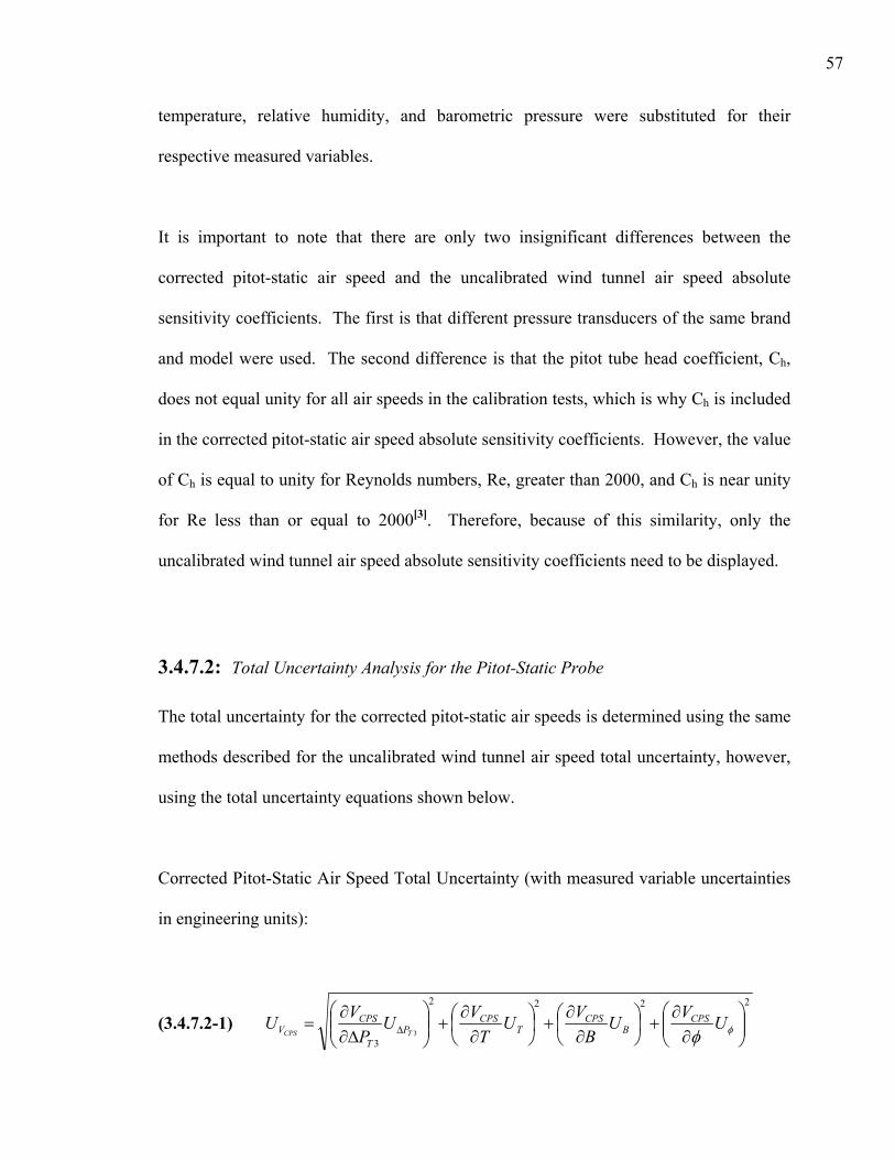
57
temperature, relative humidity, and barometric pressure were substituted for their
respective measured variables.
It is important to note that there are only two insignificant differences between the
corrected pitot-static air speed and the uncalibrated wind tunnel air speed absolute
sensitivity coefficients. The first is that different pressure transducers of the same brand
and model were used. The second difference is that the pitot tube head coefficient, Ch,
does not equal unity for all air speeds in the calibration tests, which is why Ch is included
in the corrected pitot-static air speed absolute sensitivity coefficients. However, the value
of Ch is equal to unity for Reynolds numbers, Re, greater than 2000, and Ch is near unity
for Re less than or equal to 2000[3]. Therefore, because of this similarity, only the
uncalibrated wind tunnel air speed absolute sensitivity coefficients need to be displayed.
3.4.7.2: Total Uncertainty Analysis for the Pitot-Static Probe
The total uncertainty for the corrected pitot-static air speeds is determined using the same
methods described for the uncalibrated wind tunnel air speed total uncertainty, however,
using the total uncertainty equations shown below.
Corrected Pitot-Static Air Speed Total Uncertainty (with measured variable uncertainties
in engineering units):
(3.4.7.2-1) 2222
33 ⎟⎟
⎠
⎞⎜⎜⎝
⎛∂
∂+⎟
⎠⎞
⎜⎝⎛
∂∂
+⎟⎠⎞
⎜⎝⎛
∂∂
+⎟⎟⎠
⎞⎜⎜⎝
⎛∆∂
∂= ∆ φφ
UVUB
VUT
VUP
VU CPSB
CPST
CPSP
T
CPSV TCPS

58
Corrected Pitot-Static Air Speed Total Uncertainty (with measured variable uncertainties
in units of volts):
(3.4.7.2-2) 2222
33
⎟⎟⎠
⎞⎜⎜⎝
⎛
∂∂
+⎟⎟⎠
⎞⎜⎜⎝
⎛∂
∂+⎟⎟
⎠
⎞⎜⎜⎝
⎛∂
∂+⎟
⎟⎠
⎞⎜⎜⎝
⎛
∂∂
=∆
∆φ
φV
CPSV
B
CPSV
T
CPSV
P
CPSV U
VVU
VVU
VVU
VVU
BTTP
T
CPS
3.4.8: Uncertainty Analysis Results
3.4.8.1: Wind Tunnel System
The total uncertainty results for the average uncalibrated wind tunnel air speeds in the
front, middle and back position anemometer calibration tests varied at most by 4.86 ×
10-2 m/s from each other at any given wind speed, and the results for the middle tests
always fell between that of the front and back tests. Looking at the standard deviation,
which was directly used to calculate the precision error limit of the average uncalibrated
wind tunnel air speeds, note that the maximum standard deviation for the average
uncalibrated wind tunnel air speeds in the front, middle and back position anemometer
calibration tests at any given wind speed is 4.46 × 10⁻² m/s. Taking into account that
variance (Var) is the square of the standard deviation, the maximum variance at any
given wind speed is 1.99 × 10⁻³ m2/s2. Also, even though the anemometer moved to
different positions for the front, middle and back position tests, everything regarding the
uncalibrated wind tunnel air speed remained the same. Using the fact that the setup for
all three sets of tests was the same, as well as the uncertainty calculations themselves,
only the uncertainty results for the middle position tests need to be displayed as a

59
representative of all the uncalibrated wind tunnel air speed uncertainty results. The
uncalibrated wind tunnel air speed uncertainty results for the middle position tests include
the standard deviation, variance, bias error limit, precision error limit, and total
uncertainty that are displayed below in Table 3.4.8.1-1.
Table 3.4.8.1-1: Uncertainty results of the middle position anemometer calibration tests for uncalibrated wind tunnel air speed.
Uncalibrated Wind Tunnel Air Speed, VUC, in Middle Position
VUC [m/s]
SxVUC [m/s]
VarVUC [m2/s2]
BEVUC
[m/s] PEVUC
[m/s] UVUC
[m/s] UVUC /VUC
[%]
4.25 1.89 × 10⁻² 3.56 × 10⁻⁴ 1.07 2.23 × 10-
41.07 25.1
6.15 1.51 × 10⁻² 2.28 × 10⁻⁴ 0.734 1.79 × 10-
40.734 11.9
8.24 9.99 × 10⁻³ 9.98 × 10⁻⁵ 0.549 1.19 × 10-
40.549 6.66
10.2 1.32 × 10⁻² 1.74 × 10⁻⁴ 0.442 1.54 × 10-
40.442 4.32
12.4 1.98 × 10⁻² 3.92 × 10⁻⁴ 0.366 2.34 × 10-
40.366 2.96
14.2 2.71 × 10⁻² 7.32 × 10⁻⁴ 0.318 3.21 × 10-
40.318 2.24
16.2 2.42 × 10⁻² 5.85 × 10⁻⁴ 0.280 2.83 × 10-
40.280 1.73
18.3 1.91 × 10⁻² 3.67 × 10⁻⁴ 0.248 2.26 × 10-
40.248 1.36
20.3 3.05 × 10⁻² 9.33 × 10⁻⁴ 0.224 3.58 × 10-
40.224 1.10
22.3 3.10 × 10⁻² 9.62 × 10⁻⁴ 0.205 3.66 × 10-
40.205 0.918
24.3 2.74 × 10⁻² 7.52 × 10⁻⁴ 0.189 3.22 × 10-
40.189 0.777
26.2 3.00 × 10⁻² 9.02 × 10⁻⁴ 0.175 3.55 × 10-
40.175 0.667
The total uncertainty results for the average calibrated wind tunnel air speeds in the front,
middle and back position anemometer calibration tests varied at most by 2.11 × 10⁻² m/s
from each other at any given wind speed, and the results for the middle tests always fell
between that of the front and back tests. Both the standard deviation and variance for the
average calibrated wind tunnel air speeds are equal to that of the average uncalibrated
wind tunnel air speeds, because both the average uncalibrated and calibrated wind tunnel

60
air speeds share the same raw test data. Even though the anemometer moved to different
positions for the front, middle and back position tests, which caused the wind tunnel
linear calibration equations found in Figures 4.1-1 to 4.1-3 to be significantly different,
this difference was not significant with regards to uncertainty as demonstrated above.
Also, the only difference between the front, middle and back position test uncertainty
calculations is the wind tunnel calibration slope, M, coefficient that is near unity for all of
the calibration tests. Therefore, only the uncertainty results for the middle position tests
need to be displayed as a representative of all the calibrated wind tunnel air speed
uncertainty results. The calibrated wind tunnel air speed uncertainty results for the
middle position tests include the standard deviation, variance, bias error limit, precision
error limit, and total uncertainty that are displayed below in Table 3.4.8.1-2.

61
Table 3.4.8.1-2: Uncertainty results of the middle position anemometer calibration tests for calibrated wind tunnel air speed.
Calibrated Wind Tunnel Air Speed, VC, in Middle Position
VC [m/s]
SxVC [m/s]
VarVC [m2/s2]
BEVC [m/s]
PEVC [m/s]
UVC [m/s]
UVC /VC [%]
3.99 1.89 × 10⁻² 3.56 × 10⁻⁴ 1.06 2.23 × 10⁻⁴ 1.06 26.7 5.88 1.51 × 10⁻² 2.28 × 10⁻⁴ 0.733 1.79 × 10⁻⁴ 0.733 12.5 7.98 9.99 × 10⁻³ 9.98 × 10⁻⁵ 0.548 1.19 × 10⁻⁴ 0.548 6.88 10.0 1.32 × 10⁻² 1.74 × 10⁻⁴ 0.442 1.54 × 10⁻⁴ 0.442 4.44 12.1 1.98 × 10⁻² 3.92 × 10⁻⁴ 0.366 2.33 × 10⁻⁴ 0.366 3.02 13.9 2.71 × 10⁻² 7.32 × 10⁻⁴ 0.318 3.21 × 10⁻⁴ 0.318 2.28 15.9 2.42 × 10⁻² 5.85 × 10⁻⁴ 0.279 2.83 × 10⁻⁴ 0.279 1.75 18.0 1.91 × 10⁻² 3.67 × 10⁻⁴ 0.248 2.26 × 10⁻⁴ 0.248 1.38 20.0 3.05 × 10⁻² 9.33 × 10⁻⁴ 0.224 3.58 × 10⁻⁴ 0.224 1.12 22.0 3.10 × 10⁻² 9.62 × 10⁻⁴ 0.204 3.66 × 10⁻⁴ 0.204 0.929 24.0 2.74 × 10⁻² 7.52 × 10⁻⁴ 0.188 3.22 × 10⁻⁴ 0.188 0.785 26.0 3.00 × 10⁻² 9.02 × 10⁻⁴ 0.175 3.54 × 10⁻⁴ 0.175 0.674
For comparison purposes, the uncalibrated wind tunnel air speed uncertainty and the
calibrated wind tunnel air speed uncertainty results for the middle position tests are
displayed in graphical form in Figure 3.4.8.1-1.

62
Total Uncertainty for Uncalibrated and Calibrated Wind Tunnel Air Speeds versus Uncalibrated and Calibration Wind Tunnel Air Speeds, Respectively,
for the Middle Test Position
0.00
0.20
0.40
0.60
0.80
1.00
1.20
2.0 4.0 6.0 8.0 10.0 12.0 14.0 16.0 18.0 20.0 22.0 24.0 26.0 28.0
Air Speed [m/s]
Tota
l Unc
erta
inty
[m/s
]
Uncalibrated Wind Tunnel Air Speed Middle Test Calibrated Wind Tunnel Air Speed Middle Test
Figure 3.4.8.1-1: Uncertainty results of the middle position anemometer calibration tests
for uncalibrated wind tunnel air speed and calibrated wind tunnel air speed.
3.4.8.2: Pitot-Static Probe:
The total uncertainty results for the average corrected pitot-static air speeds in the front,
middle and back position pitot-static probe calibration tests varied at most by 3.64 × 10⁻³
m/s from each other at any given wind speed, and the results for the middle tests always
fell between that of the front and back tests. Looking at the standard deviation, which
was directly used to calculate the precision error limit of the average corrected pitot-static
air speeds, note that the maximum standard deviation for the average corrected pitot-
static air speeds in the front, middle and back position anemometer calibration tests at
any given wind speed is 3.46 × 10⁻² m/s. Taking into account that variance is the square
63
of the standard deviation, the maximum variance at any given wind speed is 1.20 × 10⁻³
m2/s2. Even though the pitot-static probe moved to different positions for the front,
middle and back position tests, this difference was not significant with regards to
uncertainty as demonstrated above. Also, the only difference between the front, middle
and back position test uncertainty calculations is the pitot tube head coefficient, Ch,
which is equal to unity for Reynolds numbers, Re, greater than 2000, and Ch is near unity
for Re less than or equal to 2000[3]. Therefore, only the uncertainty results for the middle
position tests need to be displayed as a representative of all the corrected pitot-static air
speed uncertainty results. The corrected pitot-static air speed uncertainty results for the
middle position tests include the standard deviation, variance, bias error limit, precision
error limit, and total uncertainty that are displayed below in Table 3.4.8.2-1.

64
Table 3.4.8.2-1: Uncertainty results of the middle position pitot-static probe calibration tests for corrected pitot-static air speed.
Corrected Pitot-Static Air Speed, VCPS, in Middle Position
VCPS [m/s]
SxVCPS [m/s]
VarVCPS [m2/s2]
BEVCPS [m/s]
PEVCPS [m/s]
UVCPS [m/s]
UVCPS / VCPS [%]
4.00 7.77 × 10⁻³ 6.03 × 10⁻⁵ 1.41 × 10⁻¹ 9.28 × 10⁻⁵ 1.41 × 10⁻¹ 3.52 5.90 5.19 × 10⁻³ 2.69 × 10⁻⁵ 9.55 × 10⁻² 6.18 × 10⁻⁵ 9.55 × 10⁻² 1.62 7.96 1.36 × 10⁻² 1.85 × 10⁻⁴ 7.15 × 10⁻² 1.65 × 10⁻⁴ 7.15 × 10⁻² 0.899 10.0 1.36 × 10⁻² 1.84 × 10⁻⁴ 5.75 × 10⁻² 1.62 × 10⁻⁴ 5.75 × 10⁻² 0.575 12.1 1.22 × 10⁻² 1.49 × 10⁻⁴ 4.87 × 10⁻² 1.45 × 10⁻⁴ 4.87 × 10⁻² 0.402 14.0 1.55 × 10⁻² 2.41 × 10⁻⁴ 4.33 × 10⁻² 1.85 × 10⁻⁴ 4.33 × 10⁻² 0.309 16.0 1.43 × 10⁻² 2.05 × 10⁻⁴ 3.98 × 10⁻² 1.67 × 10⁻⁴ 3.98 × 10⁻² 0.249 18.0 2.15 × 10⁻² 4.63 × 10⁻⁴ 3.76 × 10⁻² 2.57 × 10⁻⁴ 3.76 × 10⁻² 0.208 20.0 2.12 × 10⁻² 4.50 × 10⁻⁴ 3.65 × 10⁻² 2.52 × 10⁻⁴ 3.65 × 10⁻² 0.182 22.1 2.71 × 10⁻² 7.35 × 10⁻⁴ 3.61 × 10⁻² 3.23 × 10⁻⁴ 3.61 × 10⁻² 0.164 24.0 1.92 × 10⁻² 3.70 × 10⁻⁴ 3.64 × 10⁻² 2.26 × 10⁻⁴ 3.64 × 10⁻² 0.151 26.0 2.55 × 10⁻² 6.53 × 10⁻⁴ 3.71 × 10⁻² 3.02 × 10⁻⁴ 3.71 × 10⁻² 0.143
In order to visualize the uncertainty trend more easily, the corrected pitot-static air speed
uncertainty results for the middle position tests are displayed in graphical form in Figure
3.4.8.2-1.

65
Corrected Pitot-Static Air Speed Total Uncertainty versus Corrected Pitot-Static Air Speed for the Middle Test Position
0.000
0.020
0.040
0.060
0.080
0.100
0.120
0.140
0.160
2.0 4.0 6.0 8.0 10.0 12.0 14.0 16.0 18.0 20.0 22.0 24.0 26.0 28.0
Air Speed [m/s]
Tota
l Unc
erta
inty
[m/s
]
Corrected Pitot-Stastic Air Speed Middle Test
Figure 3.4.8.2-1: Uncertainty results of the middle position pitot-static probe calibration
tests for corrected pitot-static air speed.
3.4.9: Uncertainty Analysis Discussion
The uncertainty analysis results for both the uncalibrated and calibrated wind tunnel air
speed were very consistent with each other. This consistency was illustrated by the fact
that the uncalibrated wind tunnel air speed total uncertainty varied at any given air speed
by no more than 4.86 × 10⁻² m/s, which is only 4.57% of UVUC or 1.14% of VUC. The
calibrated wind tunnel air speed total uncertainty, which was even more consistent, varied
at any given air speed by no more than 2.11 × 10⁻² m/s, which is only 1.99% of UVC or
0.529% of VC. The total uncertainty for the uncalibrated and calibrated wind tunnel air
speeds ranged from 0.174 m/s to 1.09 m/s. The standard deviation and variance for the

66
uncalibrated and calibrated wind tunnel air speeds ranged from 9.13 × 10⁻³ m/s to 4.46 ×
10-2 m/s and from 8.34 × 10⁻⁵ m2/s2 to 1.99 × 10⁻³ m2/s2, respectively. The uncalibrated
and calibrated wind tunnel air speeds ranged from 3.91 m/s to 26.3 m/s. Like the
uncalibrated and calibrated wind tunnel air speed total uncertainty, the total uncertainty
for the corrected pitot-static air speed tests was consistent. This consistency was
illustrated by the fact that the front, middle and back pitot-static air speed test total
uncertainties did not vary from each other at any given air speed more than 3.64 × 10⁻³
m/s, which is only 2.57% of UVCPS or 9.17 × 10⁻²% of VCPS. The total uncertainty for the
corrected pitot-static air speeds ranged from 3.69 × 10⁻² m/s to 0.144 m/s. The standard
deviation and variance for the corrected pitot-static air speeds ranged from 5.19 × 10⁻³
m/s to 3.46 × 10⁻² m/s and from 2.69 × 10⁻⁵ m2/s2 to 1.20 × 10⁻³ m2/s2, respectively. The
corrected pitot-static air speeds ranged from 3.94 m/s to 26.0 m/s. A review of the above
results shows that the factor that makes the corrected pitot-static air speed more accurate
is the range for the differential pressure transducer. Transducer #1, used to measure wind
tunnel air speed, has a range of 0 to 15 INWC, whereas Transducer #2, used to measure
pitot-static air speed, has a range of 0 to 2.5 INWC[23]. The smaller total air speed range
of Transducer #2 allows it to have greater sensitivity over the air speed range of 4 to 26
m/s than does that of Transducer #1. This greater sensitivity is the main reason why the
corrected pitot-static air speed has less uncertainty than that of the uncalibrated and
calibrated wind tunnel air speed. Therefore, for future wind tunnel air speed calibration
tests conducted over an air speed range of 4 to 26 m/s, Transducer #2 should be used in
order to achieve greater accuracy in the measured result. Besides the pressure range of
differential pressure transducers, that is a larger contributor to its overall bias error, the

67
largest contributor is the full scale range (FSR) voltage that determines the magnitude of
the DAQ error based on a given DAQ card. Therefore, the more accurate the DAQ card
is, the smaller the DAQ error will be.
FSR voltage, with respect to determining bias error for uncertainty analysis, is regarded
in industry as the most conservative value used in average error estimates and thus may
be safely substituted with the actual reading in order to get a more realistic error estimate.
This methodology applies to such error estimates as the least significant bit bias error, as
well as the calibration bias error. Using this more aggressive approach to bias error
determination would decrease the total bias error for air speed by 9 percent if Transducer
#1 (wind tunnel air speed) is used, or by 15 to 25% if Transducer #2 is used (pitot-static
air speed).
As mentioned above, the total uncertainty of the wind tunnel air speed is chiefly affected
by the differential pressure transducer calibration bias error and its DAQ error associated
with the DAQ card. Therefore, if calibration tests were needed outside of the 0 to 2.5
INWC pressure range (Transducer #2)[23], however requiring the same total uncertainty of
0.1 m/s (ASTM Requirement XII, assuming “relative uncertainty” means total
uncertainty), then both the pressure transducer and the DAQ card would have to be
replaced. A possible replacement for the pressure transducer would be the MKS Baratron
220D differential pressure transducer (0 to 15 INWC pressure range) with a calibration
uncertainty of 0.15% of the output voltage reading and a FSR output of 10 V[33, 34]. This
compares to the currently used pressure transducer (model number 239) made by Setra
68
Systems Inc. with a 0 to 15 INWC pressure range and a calibration uncertainty of 0.073%
FSR and a FSR output of 5 V[23]. A possible replacement for the DAQ card would be
the NI 9205 DAQ card with an uncertainty of 6.230 mV at a FSR of -10 to 10 V, or 3.230
mV at a FSR of -5 to 5 V[35, 36]. This compares to the currently used DAQ card (NI PCI-
6071E) made by National Instruments (NI) with an uncertainty of 14.369 mV at a FSR of
-10 to 10 V, or 5.193 mV at a FSR of -5 to 5 V[25].
4. ANEMOMETER CALIBRATION RESULTS
4.1: REGULAR CALIBRATION TEST RESULTS
The results for all eighteen regular anemometer and pitot-static probe calibration tests,
were averaged for the front, middle and back position and are shown in Figures 4.1-1 to
4.1-3.

69
Anemometer and Corrected Pitot-Static Air Speed (Reference Air Speed) versus Uncalibrated Wind Tunnel Air Speed for Tests in the Front of the Test Section
Wind Tunnel Linear Calibration Equation using the Anemometer
VREF [m/s] = ( 0.977 ) VUC [m/s] - 0.208 m/sR2 = 0.99998
Wind Tunnel Linear Calibration Equation using the Pitot-Static Tube
VREF [m/s] = ( 0.982 ) VUC [m/s] - 0.227 m/sR2 = 0.99999
0
5
10
15
20
25
30
0 5 10 15 20 25 30
Uncalibrated Wind Tunnel Air Speed, VUC (m/s)
Ref
eren
ce A
ir Sp
eed,
VR
EF (m
/s)
Anemometer Air Speed Corrected Pitot-Static Air SpeedLinear (Anemometer Air Speed) Linear (Corrected Pitot-Static Air Speed)
Figure 4.1-1: Anemometer and pitot-static probe measurements versus uncalibrated wind tunnel air speed in the front of the wind tunnel test section.

70
Anemometer and Corrected Pitot-Static Air Speed (Reference Air Speed) versus Uncalibrated Wind Tunnel Air Speed for Tests in the Middle of the Test Section
Wind Tunnel Linear Calibration Equation using the Anemometer
VREF [m/s] = ( 1.00 ) VUC [m/s] - 0.260 m/sR2 = 0.99998
Wind Tunnel Linear Calibration Equation using the Pitot-Static Tube
VREF [m/s] = ( 0.999 ) VUC [m/s] - 0.236 m/sR2 = 0.99999
0
5
10
15
20
25
30
0 5 10 15 20 25 30
Uncalibrated Wind Tunnel Air Speed, VUC (m/s)
Ref
eren
ce A
ir Sp
eed,
VR
EF (m
/s)
Anemometer Air Speed Corrected Pitot-Static Air SpeedLinear (Anemometer Air Speed) Linear (Corrected Pitot-Static Air Speed)
Figure 4.1-2: Anemometer and pitot-static probe measurements versus uncalibrated wind tunnel air speed in the middle of the wind tunnel test section.

71
Anemometer and Corrected Pitot-Static Air Speed (Reference Air Speed) versus Uncalibrated Wind Tunnel Air Speed for Tests in the Back of the Test Section
Wind Tunnel Linear Calibration Equation using the Anemometer
VREF [m/s] = ( 1.00 ) VUC [m/s] - 0.297 m/sR2 = 0.99996
Wind Tunnel Linear Calibration Equation using the Pitot-Static Tube
VREF [m/s] = ( 1.00 ) VUC [m/s] - 0.216 m/sR2 = 0.99999
0
5
10
15
20
25
30
0 5 10 15 20 25 30
Uncalibrated Wind Tunnel Air Speed, VUC (m/s)
Ref
eren
ce A
ir Sp
eed,
VR
EF (m
/s)
Anemometer Air Speed Corrected Pitot-Static Air SpeedLinear (Anemometer Air Speed) Linear (Corrected Pitot-Static Air Speed)
Figure 4.1-3: Anemometer and pitot-static probe measurements versus uncalibrated
wind tunnel air speed in the back of the wind tunnel test section.
The results of both the anemometer and pitot-static probe tests clearly show how
consistently the wind tunnel is able to measure air speed in the test section, as
demonstrated in the R2 (coefficient of determination) values in Figures 4.1-1 to 4.1-3.
However, the results also show that calibration coefficients will have to be employed
when measuring air speed at specific locations (such as the front, middle and back
position) in the test section, since the wind tunnel linear calibration equations (shown in
Figures 4.1-1 to 4.1-3), obtained by using either the anemometer or the pitot-static probe
as the reference air speed, were neither approximately equal in value nor were the slopes
equal to unity and the intercept values equal to zero. If the wind tunnel linear calibration
equations had slopes equal to unity and the intercept values were zero, the values for
wind-tunnel air speed, anemometer air speed, and pitot-static probe air speed would be in

72
agreement, and therefore the wind tunnel air speed would not require calibration
coefficients in order to satisfy the requirements for calibrating anemometers. However,
since calibration coefficients are required, the wind tunnel linear calibration equations
obtained using the anemometer in the front, middle and back test section positions will be
used to supply the calibration coefficients for anemometer calibration tests (displayed in
Table 4.1-1). For verification purposes only, the calibration coefficients from the wind
tunnel linear calibration equations obtained using the pitot-static probe in the front,
middle and back test section positions are displayed in Table 4.1-2.
Table 4.1-1: Anemometer position location compared with anemometer calibration coefficients (slope and intercept) obtained from the wind tunnel linear calibration equations in Figures 4.1-1 to 4.1-3, (where VREF = MVUC + I, is the general equation form).
Calibration Coefficients Obtained from the Wind Tunnel Linear Calibration Equations
Using the Anemometer
Position Description
Slot Number
Wind Tunnel Test Section
Position (inches)
Slope, M [unitless] Intercept, I [m/s]
Front 1 6.227 0.977 -0.208Middle 7 55.743 1.00 -0.260 Back 12 96.946 1.00 -0.297

73
Table 4.1-2: Pitot-Static probe position location compared with pitot-static probe calibration coefficients (slope and intercept) obtained from the wind tunnel linear calibration equations in Figures 4.1-1 to 4.1-3.
Calibration Coefficients Obtained from the Wind Tunnel Linear Calibration Equation
Using the Pitot-Static Tube
Position Description
Slot Number
Wind Tunnel Test Section
Position (inches)
Slope, M [unitless] Intercept, I [m/s]
Front 1 6.221 0.982 -0.227Middle 7 55.712 0.999 -0.236 Back 12 96.951 1.00 -0.216
In order to determine a possible trend for the anemometer calibration coefficients, the
length-wise position (from the front to the back of the wind tunnel test section) of the
anemometer would need to be compared against its respective calibration coefficients.
Again, for verification purposes, position measurements were taken of the pitot-static
probe as well. The positions of both the anemometer and the pitot-static probe are
referenced from Ring #2 (displayed in Figure 2.1-1) that is located just in front of the test
section. The anemometer’s position in the test section was measured from Ring #2 to the
leading edge of the anemometers propeller. The front, middle and back position for the
anemometer were at 6.227 in., 55.743 in. and 96.946 in., respectively (also displayed in
Table 4.1-1). The pitot-static probe’s position in the test section was measured from Ring
#2 to the total pressure port on the very tip of the pitot-static probe. The front, middle
and back position for the pitot-static probe were at 6.221 in., 55.712 in. and 96.951 in.,
respectively (also displayed in Table 4.1-2). With calibration coefficients coupled with
their respective position, a trend can be determined that would enable calibration

74
coefficients to be calculated for calibrating anemometers at an infinite number of test
section positions (other than at the front, middle and back positions) depending on the
particular requirements of the anemometer being calibrated. The slope calibration
coefficient trends for both the anemometer and the pitot-static probe (for verification
purposes only) are displayed below in Figure 4.1-4. The intercept calibration coefficient
trends for both the anemometer and the pitot-static probe (for verification purposes only)
are displayed below in Figure 4.1-5.
Wind Tunnel Linear Calibration Equation Slopes using Anemometer and Corrected Pitot-Static Air Speeds versus Test Section Position
0.975
0.980
0.985
0.990
0.995
1.000
1.005
0 10 20 30 40 50 60 70 80 90 100
Position (inches)
Slop
e [u
nitle
ss]
Wind Tunnel Linear Calibration Equation Slopes using Anemometer Air SpeedWind Tunnel Linear Calibration Equation Slopes using Corrected Pitot-Static Air Speed
Figure 4.1-4: Anemometer and pitot-static probe linear calibration equation slopes for the front, middle and back wind tunnel test section positions.

75
Wind Tunnel Linear Calibration Equation Intercepts using Anemometer and Corrected Pitot-Static Air Speeds versus Test Section Position
-0.300
-0.275
-0.250
-0.225
-0.200
-0.175
-0.150
0 10 20 30 40 50 60 70 80 90 100
Position (inches)
Inte
rcep
t [m
/s]
Wind Tunnel Linear Calibration Equation Intercepts using Anemometer Air SpeedWind Tunnel Linear Calibration Equation Intercepts using Corrected Pitot-Static Air Speed
Figure 4.1-5: Anemometer and pitot-static probe linear calibration equation intercepts for the front, middle and back wind tunnel test section positions.
Unfortunately, as illustrated in Figures 4.1-4 and 4.1-5, future calibration tests would
need to be conducted at several more positions, at least, along the length of the test
section in order to determine the exact nature of the trends outlined in Figures 4.1-4 and
4.1-5. Only after these future tests, will it be possible to determine, by means of an
empirical formula, the calibration coefficients related to test section position. However,
once the empirical calibration coefficient formulas (for both slope and intercept) are
determined, anemometer calibrations will be able to be performed at any position (along
the length of the test section) with the same accuracy that is afforded to the front, middle
and back positions because of their calibration coefficients. Note that when the
calibration coefficients are applied to the uncalibrated wind tunnel air speed, the now

76
calibrated wind tunnel air speed values are in agreement with the anemometer air speed
values and pitot-static probe air speed values (for verification purposes only) as
illustrated in Figures 4.1-6 to 4.1-8. The agreement between the calibrated wind tunnel
air speed with the anemometer and pitot-static probe air speeds is further displayed by the
fact that the wind tunnel linear calibration verification equations have slopes equal to
unity and intercept values equal to zero (as shown in Figures 4.1-6 to 4.1-8).
Anemometer and Corrected Pitot-Static Air Speed (Reference Air Speed) versus Calibrated Wind Tunnel Air Speed for Tests in the Front of the Test Section
Wind Tunnel Linear Calibration Verification Equation using the Anemometer
VREF [m/s] = ( 1.00 ) VC [m/s] - 0.00 m/sR2 = 0.99998
Wind Tunnel Linear Calibration Verification Equation using the Pitot-Static Tube
VREF [m/s] = ( 1.00 ) VC [m/s] + 0.00 m/sR2 = 0.99999
0
5
10
15
20
25
30
0 5 10 15 20 25 30
Calibrated Wind Tunnel Air Speed, VC (m/s)
Ref
eren
ce A
ir Sp
eed,
VR
EF (m
/s)
Anemometer Air Speed Corrected Pitot-Static Air SpeedLinear (Anemometer Air Speed) Linear (Corrected Pitot-Static Air Speed)
Figure 4.1-6: Anemometer and pitot-static probe measurements versus calibrated wind tunnel air speed in the front of the wind tunnel test section.

77
Anemometer and Corrected Pitot-Static Air Speed (Reference Air Speed) versus Calibrated Wind Tunnel Air Speed for Tests in the Middle of the Test Section
Wind Tunnel Linear Calibration Verification Equation using the Anemometer
VREF [m/s] = ( 1.00 ) VC [m/s] + 0.00 m/sR2 = 0.99998
Wind Tunnel Linear Calibration Verification Equation using the Pitot-Static Tube
VREF [m/s] = ( 1.00 ) VC [m/s] - 0.00 m/sR2 = 0.99999
0
5
10
15
20
25
30
0 5 10 15 20 25 30
Calibrated Wind Tunnel Air Speed, VC (m/s)
Ref
eren
ce A
ir Sp
eed,
VR
EF (m
/s)
Anemometer Air Speed Corrected Pitot-Static Air SpeedLinear (Anemometer Air Speed) Linear (Corrected Pitot-Static Air Speed)
Figure 4.1-7: Anemometer and pitot-static probe measurements versus calibrated wind
tunnel air speed in the middle of the wind tunnel test section.

78
Anemometer and Corrected Pitot-Static Air Speed (Reference Air Speed) versus Calibrated Wind Tunnel Air Speed for Tests in the Back of the Test Section
Wind Tunnel Linear Calibration Verification Equation using the Anemometer
VREF [m/s] = ( 1.00 ) VC [m/s] + 0.00 m/sR2 = 0.99996
Wind Tunnel Linear Calibration Verification Equation using the Pitot-Static Tube
VREF [m/s] = ( 1.00 ) VC [m/s] - 0.00 m/sR2 = 0.99999
0
5
10
15
20
25
30
0 5 10 15 20 25 30
Calibrated Wind Tunnel Air Speed, VC (m/s)
Ref
eren
ce A
ir Sp
eed,
VR
EF (m
/s)
Anemometer Air Speed Corrected Pitot-Static Air SpeedLinear (Anemometer Air Speed) Linear (Corrected Pitot-Static Air Speed)
Figure 4.1-8: Anemometer and pitot-static probe measurements versus calibrated wind
tunnel air speed in the back of the wind-tunnel test section.
In order to further confirm the success of the calibration test, linear transfer functions
where determined for the anemometer at the front, middle and back test positions using
both the uncalibrated and calibrated wind tunnel air speeds as shown in Figures 4.1-9 to
4.1-11. The standard for comparison against the linear transfer functions determined for
the front, middle and back position tests is the linear transfer function, VREF [m/s] = (
2.93 × 10⁻² m/(s·Hz) ) f [Hz] + 3.89 × 10⁻² m/s, obtained from the anemometer calibration
data listed in the calibration certificate[20] (provided by OTECH Engineering) that is
shown in Figure A-1 in Appendix A. When comparing the calibrated linear transfer
functions (found in Figures 4.1-9 to 4.1-11) to the OTECH Engineering anemometer

79
linear transfer function, the slopes are off by at most -0.341%, and the intercepts are off
by 1.89 × 10⁻² m/s.
Uncalibrated and Calibrated Wind Tunnel Air Speed (Reference Air Speed) versus Anemometer Frequency for Tests in the Front of the Test Section
(with the OTECH Engineering calibration curve displayed)
Uncalibrated VREF Linear Transfer Function
VREF [m/s] = ( 2.99 x 10⁻² m/(s·Hz) ) f [Hz] + 0.269 m/sR2 = 1.00000
Calibrated VREF Linear Transfer Function
VREF [m/s] = ( 2.92 x 10⁻² m/(s·Hz) ) f [Hz] + ( 5.43 x 10⁻² ) m/sR2 = 1.00000
OTECH Engineering VREF Linear Transfer Function
VREF [m/s] = ( 2.93 x 10⁻² m/(s·Hz) ) f [Hz] + ( 3.89 x 10⁻² ) m/sR2 = 0.99998
0
5
10
15
20
25
30
0 100 200 300 400 500 600 700 800 900 1000
Anemometer Frequency, f (Hz)
Ref
eren
ce A
ir Sp
eed,
VR
EF (m
/s)
Uncalibrated Wind Tunnel Air Speed Calibrated Wind Tunnel Air SpeedOTECH Engineering Reference Air Speed Linear (Uncalibrated Wind Tunnel Air Speed)Linear (Calibrated Wind Tunnel Air Speed) Linear (OTECH Engineering Reference Air Speed)
Figure 4.1-9: Uncalibrated and calibrated wind tunnel air speed versus anemometer frequency for tests in the front of the wind-tunnel test section (with the OTECH Engineering calibration curve displayed for comparison).

80
Uncalibrated and Calibrated Wind Tunnel Air Speed (Reference Air Speed) versus Anemometer Frequency for Tests in the Middle of the Test Section
(with the OTECH Engineering calibration curve displayed)
Uncalibrated VREF Linear Transfer Function
VREF [m/s] = ( 2.92 x 10⁻² m/(s·Hz) ) f [Hz] + 0.318 m/sR2 = 1.00000
Calibrated VREF Linear Transfer Function
VREF [m/s] = ( 2.92 x 10⁻² m/(s·Hz) ) f [Hz] + ( 5.78 x 10⁻² ) m/sR2 = 1.00000
OTECH Engineering VREF Linear Transfer Function
VREF [m/s] = ( 2.93 x 10⁻² m/(s·Hz) ) f [Hz] + ( 3.89 x 10⁻² ) m/sR2 = 0.99998
0
5
10
15
20
25
30
0 100 200 300 400 500 600 700 800 900 1000
Anemometer Frequency, f (Hz)
Ref
eren
ce A
ir Sp
eed,
VR
EF (m
/s)
Uncalibrated Wind Tunnel Air Speed Calibrated Wind Tunnel Air SpeedOTECH Engineering Reference Air Speed Linear (Uncalibrated Wind Tunnel Air Speed)Linear (Calibrated Wind Tunnel Air Speed) Linear (OTECH Engineering Reference Air Speed)
Figure 4.1-10: Uncalibrated and calibrated wind tunnel air speed versus anemometer frequency for tests in the middle of the wind tunnel test section (with the OTECH Engineering calibration curve displayed for comparison).

81
Uncalibrated and Calibrated Wind Tunnel Air Speed (Reference Air Speed) versus Anemometer Frequency for Tests in the Back of the Test Section
(with the OTECH Engineering calibration curve displayed)
Uncalibrated VREF Linear Transfer Function
VREF [m/s] = ( 2.91 x 10⁻² m/(s·Hz) ) f [Hz] + 0.351 m/sR2 = 0.99999
Calibrated VREF Linear Transfer Function
VREF [m/s] = ( 2.92 x 10⁻² m/(s·Hz) ) f [Hz] + ( 5.52 x 10⁻² ) m/sR2 = 0.99999
OTECH Engineering VREF Linear Transfer Function
VREF [m/s] = ( 2.93 x 10⁻² m/(s·Hz) ) f [Hz] + ( 3.89 x 10⁻² ) m/sR2 = 0.99998
0
5
10
15
20
25
30
0 100 200 300 400 500 600 700 800 900 1000
Anemometer Frequency, f (Hz)
Ref
eren
ce A
ir Sp
eed,
VR
EF (m
/s)
Uncalibrated Wind Tunnel Air Speed Calibrated Wind Tunnel Air SpeedOTECH Engineering Reference Air Speed Linear (Uncalibrated Wind Tunnel Air Speed)Linear (Calibrated Wind Tunnel Air Speed) Linear (OTECH Engineering Reference Air Speed)
Figure 4.1-11: Uncalibrated and calibrated wind tunnel air speed versus anemometer frequency for tests in the back of the wind tunnel test section (with the OTECH Engineering calibration curve displayed for comparison).
4.2: HYSTERESIS CALIBRATION TEST RESULTS
The six hysteresis calibration tests for the anemometer and pitot-static probe were used to
determine how consistently the UCD AWT can reach a desired air speed when either
increasing air speed or decreasing air speed in order to achieve the desired air speed. The
hysteresis tests determined that the maximum difference for a desired air speed is 8.55 ×
10-2 m/s for wind tunnel air speed (uncalibrated and calibrated), 9.50 × 10⁻² m/s for
anemometer air speed, and 4.95 × 10⁻² m/s for pitot-static probe air speed. The desired
air speeds used to calculate the maximum difference for a desired air speed were
achieved by first increasing air speed to the desired air speed, then passing the desired air

82
speed and then decreasing air speed to the desired air speed within a given hysteresis
calibration test. The maximum difference for a desired air speed was calculated by
subtracting the value of the desired air speed measured after decreasing air speed from
the desired air speed measured after increasing air speed.
The results for the hysteresis tests also showed that the difference between a given
desired air speed achieved when the air speed is increasing and again when it is
decreasing is random in nature. In other words, the desired air speed achieved when the
air speed is increasing is not always greater (positive in sign) in value than the exact same
desired air speed achieved when the air speed is decreasing. Taking into consideration
that the maximum difference values for wind tunnel air speed, anemometer air speed, and
pitot-static probe air speed are significantly less than the requirement that the wind tunnel
maintain a given air speed within ±0.2 m/s, as well as the random nature of the sign on
the difference values, suggests that the wind tunnel air speed, anemometer air speed, and
pitot-static probe air speed measurements have a negligible hysteresis.
5. DISCUSSION
The wind-tunnel calibration results mentioned in the previous section bring up an
important point that the tests were consistent enough to determine coefficients that have
been applied to the main calibration program, and thus enabling the program to meet the
calibration requirements.

83
The UCD AWT’s ability to calibrate anemometers was determined by its ability to satisfy
previously mentioned requirements in the following previously mentioned anemometer
calibration standards: the “Standard Test Method for Determining the Performance of a
Cup Anemometer or Propeller Anemometer” (ASTM D 5096-02)[19] and the “Power
Performance Measurements of Electricity Producing Wind Turbines” (IEC 61400-12-
1)[2].
The following are explanations of how the anemometer calibration requirements
(displayed below in italics) selected from the “Standard Test Method for Determining the
Performance of a Cup Anemometer or Propeller Anemometer” (ASTM D 5096-02)[19]
were met:
ASTM Requirement I. A linear transfer function is determined for the anemometer
being calibrated by measuring both the wind tunnel’s air speed and the anemometer’s
frequency of rotation for a sequence of air speeds that fall within the anemometers
working air speed range. The linear transfer function is calculated using the linear
regression method.
In order to further confirm the success of the calibration test, linear transfer functions
where determined for the anemometer at the front, middle and back test positions
using both the uncalibrated and calibrated wind tunnel air speeds as shown in Figures
4.1-9 to 4.1-11. The standard for comparison against the linear transfer functions
determined for the front, middle and back position tests is the linear transfer function,
VREF [m/s] = ( 2.93 × 10⁻² m/(s·Hz) ) f [Hz] + 3.89 × 10⁻² m/s, obtained from the
anemometer calibration data found in the calibration certificate[20] (provided by

84
OTECH Engineering) that is shown in Figure A-1 in Appendix A. The calibrated
linear transfer functions for anemometer tested at the front, middle and back test
positions are as follows, respectively: VREF [m/s] = ( 2.92 × 10⁻² m/(s·Hz) ) f [Hz] +
5.43 × 10⁻² m/s, VREF [m/s] = ( 2.92 × 10⁻² m/(s·Hz) ) f [Hz] + 5.78 × 10⁻² m/s, VREF
[m/s] = ( 2.92 × 10⁻² m/(s·Hz) ) f [Hz] + 5.52 × 10⁻² m/s. All of the above mentioned
linear transfer functions were determined for the NIST traceable anemometer, by
measuring both the wind tunnel’s air speed and the anemometer’s frequency of
rotation for a sequence of air speeds that fall within the anemometer’s working air
speed range. The linear transfer functions were all calculated using the linear
regression method.
ASTM Requirement II. The resolution of both the wind tunnel and anemometer
measured air speeds must be at least at a minimum of 0.02 m/s.
The resolution of both the wind tunnel and anemometer measured air speeds were at
0.001 m/s, which is far better than the minimum of 0.02 m/s.
ASTM Requirement III. The resolution of measuring the anemometer’s angle of
attack with respect to being parallel with the wind tunnel’s air flow has to be at least
0.5°. This is for angles of attack that deviate from parallel to the air flow.
The anemometer was aligned using the laser level method mentioned in the “3.3.1:
Anemometer or Pitot-Static Probe Setup” section. This method has a resolution of
0.01° which exceeds the minimum required resolution of 0.5°. However, the 0.5°
resolution is only a requirement if calibration tests are perform that deviate from
parallel to the air flow. At the UCD AWT, calibration tests were only performed
parallel to the air flow.

85
ASTM Requirement IV. The DAQ system must have a sampling rate of at least 100
samples per second (S/s) for a given data channel.
The wind tunnel DAQ system acquired 3,000 samples per second per channel for the
main calibration program which far exceeds the minimum sampling rate of at least
100 samples per second for a given data channel.
ASTM Requirement V. The frontal area of the anemometer and its mounting
structure inside the test section must be less than 5% of the cross-sectional area of
the test section.
The frontal area of the anemometer and its mounting structure inside the test section
was 3.5% (which is less than the required 5%) of the cross-sectional area of the test
section.
ASTM Requirement VI. The wind tunnel used for the anemometer calibration test
must be able to operate from zero to 50% of the anemometers working air speed
range, while being able to maintain a given air speed within ±0.2 m/s.
The UCD AWT has a near zero mph idle speed and a maximum speed of 165 mph in
the test section[24], whereas the anemometer used in the calibration test has a
maximum operational speed of 100 mph. Thus, the wind tunnel far exceeds the
minimum top speed of 50% of the anemometer’s working air speed range, and the
wind tunnel is able to maintain speeds within ±0.05 m/s, which is more accurate than
the minimum requirement of ±0.2 m/s.
ASTM Requirement VII. Calibration speeds must be verified with a NIST traceable
device, such as a calibrated anemometer.

86
The calibration tests were performed with a pre-calibrated NIST traceable
anemometer (provided by OTECH Engineering), which was used to verify the wind
tunnels readiness to calibrate anemometers.
ASTM Requirement VIII. The wind tunnel being used for anemometer calibration
must have turbulence levels less than 1% throughout the test section, while
maintaining a relatively constant air flow profile.
The wind tunnel being used for anemometer calibration has turbulence levels in the
test section established to be less than or equal to 0.1% for the initial 80% of the test
section throughout the wind tunnel’s velocity range, which exceeds the required 1%
of turbulence levels[24]. Note that the initial 80% of the test section includes all of the
three anemometer test positions (front, middle, and back slot position).
ASTM Requirement IX. The air density within the test section must be measured for
each independent air speed measurement. Thus the temperature, relative humidity
and barometric pressure need to measured inside the test section of the wind tunnel.
The UCD AWT has an operational temperature transmitter, relative humidity
transmitter and barometric pressure transducer installed that when coupled with the
calibration program in LabVIEW is able to calculate the air density within the test
section for each independent air speed measurement.
ASTM Requirement X. Measurements must be taken of the wind tunnel’s air speed
and the anemometer’s rotational frequency at the same desired air speeds both in and
ascending and in a descending sequence.
Regular calibration tests were performed that measure the wind tunnel’s air speed and
the anemometer’s rotational frequency at the same desired air speeds both in an

87
ascending and in a descending sequence, thus satisfying the requirement. It should be
clear that only the measurements need to be taken at the same desired air speed, and
that the desired air speeds do not need to be the same in the ascending and descending
sequence.
ASTM Requirement XI. Once the wind tunnel’s air speed has reached equilibrium
at a given desired air speed, measure and record for 30 to 100 seconds.
Once the wind tunnel’s air speed had reached equilibrium at a given desired air speed,
measurements were recorded for 30 seconds which meets the minimum requirement.
ASTM Requirement XII. A required relative accuracy of 0.1 m/s for the anemometer
that is dependent on the accuracies of the wind tunnel and its measurement system.
Note that this requirement is heavily subjective since the term “relative accuracy”
was not clearly defined.
Sense the term “relative accuracy” was not clearly defined, the requirement of
meeting a relative accuracy of 0.1 m/s for the anemometer could neither be
qualitatively nor quantitatively satisfied, and thus this requirement could not be
included as part of the anemometer calibration requirements for the UCD AWT.
The following are explanations of how the anemometer calibration requirements
(displayed below in italics) selected from the “Power Performance Measurements of
Electricity Producing Wind Turbines” (IEC 61400-12-1)[2] were met:
IEC Requirement I. The frontal area of the anemometer and its mounting structure
inside the test section must be less than 5% of the cross-sectional area of the test
section for a closed test section.
88
Just as for the ASTM Requirement V, the frontal area of the anemometer and its
mounting structure inside the test section was 3.5% (which is less than the required
5%) of the cross-sectional area of the test section.
IEC Requirement II. The wind tunnel’s anemometer calibration results must agree
with another testing facilities’ average calibration results within 1% over the range
of 4 to 16 m/s.
The UCD AWT anemometer calibration test results agree with OTECH
Engineering’s test results within 1% over a range of 4 to 26 m/s, which exceeds the
required range and meets the required percentage of agreement. However, the UCD
AWT is only able to meet this requirement with regards to the front and middle
calibrated anemometer calibration tests. The back test results agree with OTECH
Engineering’s test results within 1.71% over a range of 4 to 26 m/s, which falls just
outside of the required agreement to be within 1% over a range of 4 to 16 m/s.
However, if Transducer #1 were switched with Transducer #2, the front, middle and
back test results would all agree with OTECH Engineering’s test results within 1%
over a range of 4 to 26 m/s. It should be noted that the percent difference between the
UCD AWT and the OTECH Engineering test results is highest between 4 to 12 m/s
and then drops off significantly thereafter.
IEC Requirement III. The maximum deviation from parallel to the air flow that the
anemometer is allowed is 1°.
Taking into account the worst case for measurement, the maximum deviation would
be about 0.5° from parallel to the air flow, which exceeds the requirement of only 1°
of deviation from parallel.

89
IEC Requirement IV. The calibration speed range shall be from 4 to 16 m/s and
performed in both an ascending and descending sequence of air speeds, in intervals
of 1 m/s or less. Note that the 1 m/s intervals can be achieved with 2 m/s intervals
that are offset by 1 m/s from the ascending to the descending sequence of air speeds.
The calibration speed range sequence went from 4 to 26 m/s in 2 m/s intervals, which
exceeds the overall speed range of 4 to 16 m/s. However, the 2 m/s intervals were
used instead of the 1 m/s intervals because the linearity of the results was checked
against IEC Requirement VI. Under IEC Requirement VI, calibration results are only
considered valid if they obtain an R2 value of more than 0.99990 (or R greater than
0.99995).
IEC Requirement V. Stable air flow can be determined if two consecutive 30 second
averages at the same air speed vary a maximum of 0.05 m/s from each other.
The air flow in the test section stabilized to a maximum variance of 0.05 m/s and then
the program waited 30 seconds before recording measurements, which meets the
minimum requirement for air flow stability.
IEC Requirement VI. Calibration data should be considered invalid if the correlation
coefficient, R, is less than 0.99995 or R2 is less than 0.99990.
All calibration test results maintained a linear correlation coefficient, R, greater than
0.99995 (the minimum requirement).

90
6. CONCLUSIONS AND RECOMMENDATIONS
Do to the fact that the anemometer tests met all of the calibration requirements mentioned
in the “5. Discussion” section, the UCD AWT is ready to accurately perform calibration
tests for non-calibrated anemometers according to the requirements set forth in “Standard
Test Method for Determining the Performance of a Cup Anemometer or Propeller
Anemometer” (ASTM D 5096-02)[19] and in “Power Performance Measurements of
Electricity Producing Wind Turbines” (IEC 61400-12-1)[2]. However, note that the UCD
AWT’s ability to calibrate anemometers is conditional in that all calibrations must be
performed in the front or middle test position, as the requirements were not fully met by
the calibration tests performed in the back position. However, if Transducer #1 were
exchanged with Transducer #2, calibration tests could be performed at any position in the
wind tunnel test section. Therefore, it is recommended for future calibration tests that
Transducer #2 be used in place of Transducer #1 when conducting tests in the 4 to 26 m/s
range. By making this modification to the wind tunnel system, the ASTM Requirement
XII (assuming “relative uncertainty” means total uncertainty) of maintaining a total
uncertainty of 0.1 m/s or below, would be met, thus making the UCD AWT
unconditionally ready to calibrate anemometers with regards to all requirements.
Future calibration tests would also need to be conducted at several more positions along
the length of the test section in order to determine the exact nature of the trends outlined
in Figures 4.1-4 and 4.1-5. Only after these future tests, will it be possible to determine,
by means of an empirical formula, the calibration coefficients related to test section
position.
91
7. REFERENCES
[1] White, Frank M. “Viscous Fluid Flow”, Third Edition. New York, New York: The McGraw-Hill Companies, Inc., 2006.
[2] IEC [International Electrotechnical Commission]. IEC 61400-12-1 first edition
2005-12: Wind turbines – Part 12-1: Power performance measurements of electricity producing wind turbines. Geneva, Switzerland: International Electrotechnical Commission, 2005.
[3] Barlow, Jewel B., William H. Rae, Jr., and Alan Pope. “Low-Speed Wind Tunnel
Testing”, Third Edition. New York, New York: John Wiley & Sons, Inc., 1999. [4] Serway, Raymond A., and John W. Jewett, Jr. "Physics for Scientists and
Engineers", 6th edition. Belmont, California: Brooks/Cole--Thomson Learning, 2004.
[5] Silberberg, Martin S. "Chemistry-The Molecular Nature of Matter and Change",
Second edition. Boston, Massachusetts: The McGraw-Hill Companies, Inc., 2000.
[6] Blevins, Robert D. "Applied Fluid Dynamics Handbook". New York, New
York: Van Nostrand Reinhold Company Inc., 1984. [7] White, Frank M. “Fluid Mechanics”, Third Edition. New York, New York:
McGraw-Hill, Inc., 1994. [8] Hilsenrath, Joseph, et al. “Tables of Thermodynamic and Transport Properties of
Air, Argon, Carbon Dioxide, Carbon Monoxide, Hydrogen, Nitrogen, Oxygen, and Steam”. New York, New York: Pergamon Press, 1960.
[9] Manwell, J.F., J.G. McGowan, and A.L. Rogers. “Wind Energy Explained:
Theory, Design and Application”. West Sussex, England: John Wiley & Sons, Ltd., 2002.
[10] Dines, William Henry. “Anemometer”. EBook of Encyclopaedia Britannica,
11th Edition, Volume 2, Part 1, Slice 1. Released: October 8, 2004. Updated: February 22, 2005. Retrieved: August 30, 2009 <http://www.gutenberg.org/files/13600/13600-h/13600-h.htm>.
[11] Coquilla, Rachael. “Anemometers for Wind Energy Applications”. Wind Power
Engineering course lecture, University of California, Davis. October 19, 2006.

92
[12] Standard Sensors. NRG Systems. Retrieved: August 30, 2009 <http://www.nrgsystems.com/AllProducts/SensorsandTurbineControl/StandardSensors.aspx>.
[13] Turbine Control Sensors. NRG Systems. Retrieved: August 30, 2009
<http://www.nrgsystems.com/AllProducts/SensorsandTurbineControl/TurbineControlSensors.aspx>.
[14] Kristensen, L. “The Perennial Cup Anemometer”. Wind Energy, Volume 2,
Issue 1 (1999): 59-75. Retrieved from <http://www3.interscience.wiley.com/cgi-bin/fulltext/63001720/PDFSTART?CRETRY=1&SRETRY=0>.
[15] 05103, 05103-45, 05106, and 05305 R.M. Young Wind Monitors Instruction
Manual. Logan, Utah: Campbell Scientific, Inc., 2009. Retrieved: September 6, 2009 <http://www.campbellsci.com/documents/manuals/05103.pdf>.
[16] Model 05103 Wind Monitor, Rev: H080905, Manual PN 05103-90. Traverse
City, Michigan: R.M. Young Company. Received via email from Dennis F. Sanderson <[email protected]> on May 13, 2009.
[17] Wind Monitor. R. M. Young Company. Retrieved: September 6, 2009
<http://www.youngusa.com/products/7/5.html>. [18] Gill UVW Anemometer. R. M. Young Company. Retrieved: September 6, 2009
< http://www.youngusa.com/products/7/50.html>. [19] ASTM [American Society for Testing and Materials]. ASTM D 5096-02:
Standard Test Method for Determining the Performance of a Cup Anemometer or Propeller Anemometer. West Conshohocken, Pennsylvania: American Society for Testing and Materials, 2002.
[20] Coquilla, Rachael. “Anemometer Calibration Report”. Davis, California:
OTECH Engineering Inc., January 16, 2009.
[21] “Model 27106DR Gill Propeller Anemometer Manual PN 27106DR-90”. Traverse City, Michigan: R.M. Young Company, 2003.
[22] “Model Number PDD-24-G-21-KL Straight Dimension Drawing”. Amherst,
New Hampshire: United Sensor Corporation, Faxed November 6, 1998. [23] Test & Measurement: Model 239/C239: data sheet. Setra Systems, Inc.
Retrieved: May 16, 2009 <http://www.setra.com/tra/pro/pdf/239.pdf>.
[24] UC Davis Aeronautical Wind Tunnel Facility. Mechanical and Aeronautical Engineering Department, University of California, Davis. Retrieved: March 28, 2009 <http://windtunnel.engr.ucdavis.edu/>.

93
[25] NI PCI-6071E: Data Sheet. National Instruments. Retrieved: May 16, 2009 <http://www.ni.com/pdf/products/us/4daqsc199-201_ETC_212-213.pdf>.
[26] Munson, Bruce R., Donald F. Young, and Theodore H. Okiishi. “Fundamentals
of Fluid Mechanics”, Fourth Edition. Hoboken, New Jersey: John Wiley & Sons, Inc., 2002.
[27] Relative Humidity/Temperature Transmitters for Duct or Wall Mounting:
HX94AC and HX94AV Series: Specs. Omega Engineering, Inc. Retrieved: September 7, 2009 <http://www.omega.com/Temperature/pdf/HX94AC_HX94AV.pdf>.
[28] Barometric Pressure Measurement: Model 270: data sheet. Setra Systems, Inc.
Retrieved: May 16, 2009 <http://www.setra.com/tra/pro/pdf/270.pdf>. [29] “Calibration Certificate” Serial No. 973205. Boxborough, Massachusetts: Setra
Systems, Inc., October 22, 1998. [30] Coquilla, Rachael V., John Obermeier, and Bruce R. White. “Calibration
Procedures and Uncertainty in Wind Power Anemometers”. Wind Engineering, Volume 31, Number 5 (2007): 303-316.
[31] Coleman, Hugh W., and W. Glenn Steele, Jr. “Experimentation and Uncertainty
Analysis for Engineers”. New York: John Wiley and Sons, 1989. [32] Baker, Jonathon Paul. “Experimental Investigation into the Effectiveness of a
Microtab Aerodynamic Load Control System”. Master of Science Thesis. University of California, Davis, 2005.
[33] 220DD Baratron Differential Capacitance Manometer (0.1-1000 Torr) NEMA1
Housing, Temperature Controlled to 45 degrees C: 220DD data sheet. MKS Instruments. Retrieved: July 19, 2009 <http://www.mksinst.com/docs/UR/220dif.pdf>.
[34] 220DD Baratron Differential Capacitance Manometer (0.1-1000 Torr) NEMA1
Housing, Temperature Controlled to 45 degrees C: Baratron General Purpose & High Accuracy selection guide. MKS Instruments. Retrieved: July 19, 2009 <http://www.mksinst.com/docs/UR/barselec.pdf>.
[35] NI 9205: Data Sheet. National Instruments. Retrieved: February 21, 2010
<http://sine.ni.com/ds/app/doc/p/id/ds-190/lang/en>. [36] NI 9205: Detailed Specifications: NI 9205 Operating Instructions and
Specifications. National Instruments. Retrieved: February 21, 2010 <http://www.ni.com/pdf/manuals/374188d.pdf>.
94
[37] “Calibration Certificate” Serial No. 972923. Boxborough, Massachusetts: Setra Systems, Inc., October 20, 1998.
[38] “Calibration Certificate” Serial No. 3231233. Boxborough, Massachusetts: Setra
Systems, Inc., May 20, 2007. [39] “Certificate of Calibration for UC Davis” Serial #0701004. Bridgeport, New
Jersey: Omega Engineering, Inc., March 13, 2009. [40] “Calibration Certificate” Serial No. 3271298. Boxborough, Massachusetts: Setra
Systems, Inc., May 30, 2007.

95
8. APPENDIX A: CALIBRATED RM YOUNG PROPELLER ANEMOMETER
Figure A-1: NIST Traceable anemometer calibration certificate provided by OTECH Engineering Incorporated[20].

96
Figure A-2: User’s manual for the RM Young anemometer (Model Number 27106DR), page 1 of 5[21].

97
Figure A-3: User’s manual for the RM Young anemometer (Model Number 27106DR), page 2 of 5[21].
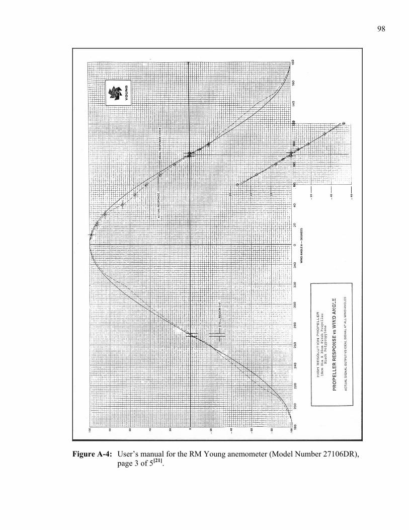
98
Figure A-4: User’s manual for the RM Young anemometer (Model Number 27106DR), page 3 of 5[21].

99
Figure A-5: User’s manual for the RM Young anemometer (Model Number 27106DR), page 4 of 5[21].

100
Figure A-6: User’s manual for the RM Young anemometer (Model Number 27106DR), page 5 of 5[21].

101
9. APPENDIX B: PITOT-STATIC PROBE
Figure B-1: Original dimensioned drawing of the pitot-static probe[22].

102
10. APPENDIX C: WIND TUNNEL INSTRUMENT SPECIFICATIONS
Table C-1: Current setup of all data cables wired to the SCB-100 connector box.
Bundle Channel DAQ Pin
(Computer Assigned)
DAQ Pin (Location in SCB-100
Connector Box)Wire Color/Description Channel Name Type Input/Output Voltage
Range
1 AOGND N/A 23 Black AO Ground Ground N/A 01 +5V N/A 34 Orange Positive 5 Volt Signal Analog N/A 5 V1 DAC0OUT N/A 20 Brown Motor Velocity Analog Output ± 5 V1 DIO0 N/A 25 Green Select 1 Binary Output N/A1 DIO1 N/A 27 White Select 2 Binary Output N/A1 DIO2 N/A 29 Red Motor On Binary Output N/A1 DGND N/A 33 Grey Digital Ground Ground N/A 02 ACH16(PC7) 51 51 White Delta P-P Differential (+) Input 0 to 5 V2 ACH24(GND) 52 52 Green Delta P-P Differential (-) Input 02 ACH16(PC7) 51 51 White T3 15 inchH2O Differential (+) Input -1 to 5 V2 ACH24(GND) 52 52 Green T3 15 inchH2O Differential (-) Input 02 ACH17(PC6) 53 53 Black Delta P-T = T1 15 inchH2O Differential (+) Input 0 to 5 V2 ACH25(GND) 54 54 Red Delta P-T = T1 15 inchH2O Differential (-) Input 03 ACH22(PC1) 63 63 Black Delta P-3 = T2 2_5 inchH2O Differential (+) Input ± 2.5 V3 ACH30(GND) 64 64 Red Delta P-3 = T2 2_5 inchH2O Differential (-) Input 03 ACH23(PC0) 65 65 White Barometric Pressure Differential (+) Input 0 to 5 V3 ACH31(GND) 66 66 Green Barometric Pressure Differential (-) Input 04 AIGND 76 [AIGND(GND)] 2 [AIGND] Black AI Ground Ground N/A 04 ACH18(PC5) 55 55 Green Psi Single Ended Input ± 5 V4 ACH19(PC4) 57 57 White Alpha Single Ended Input ± 5 V4 ACH20(PC3) 59 59 Blue Y Single Ended Input 0 to 4 V4 ACH21(PC2) 61 61 Red Z Single Ended Input 0 to 4 V5 AIGND 2 [AIGND] 1 [AIGND] Dark Grey AI Ground Ground N/A 05 ACH6 15 15 Yellow Lift-BIC Single Ended Input ± 5 V5 ACH0 3 3 Brown Lift-AIC Single Ended Input ± 5 V5 ACH7 17 17 Light Purple Drag-BIC Single Ended Input ± 5 V5 ACH1 5 5 Green Drag-AIC Single Ended Input ± 5 V5 ACH8 4 4 Beige Side Force-BIC Single Ended Input ± 5 V5 ACH2 7 7 Brown with White Stripe Side Force-AIC Single Ended Input ± 5 V5 ACH10 8 8 Light Grey M-Yaw-BIC Single Ended Input ± 5 V5 ACH4 11 11 Light Red M-Yaw-AIC Single Ended Input ± 5 V5 ACH9 6 6 White with Brown Stripe M-Roll-BIC Single Ended Input ± 5 V5 ACH3 9 9 White M-Roll-AIC Single Ended Input ± 5 V5 ACH5 13 13 Light Orange M-Pitch-BIC Single Ended Input ± 5 V5 ACH11 10 10 Blue M-Pitch-AIC Single Ended Input ± 5 V6 DGND N/A 24 Black Digital Ground Ground N/A 06 DIO4 N/A 26 Blue Fan CPU Takeover Digital Output N/A6 DIO5 N/A 28 Green with Black Stripe Fan Running Digital Input N/A6 DIO6 N/A 30 Orange with Black Stripe Fan Up To Speed Digital Input N/A6 DGND N/A 24 Thick Green Wire (Shielding) Digital Ground Ground N/A 07 DAC1OUT N/A 21 Green Fan Speed Output Analog Output 0 to 10 V7 AOGND N/A 23 Black AO Ground N/A 07 AOGND N/A 23 Non-insulated wire (Shielding) AO Ground N/A 07 ACH33(PB6) 69 69 White Fan Speed Return Differential (+) Input -1 to 10 V7 ACH41(GND) 70 70 Black Fan Speed Return Differential (-) Input 08 ACH34(PB5) 71 71 Black Temperature Differential (+) Input 0 to 1 V8 ACH42(GND) 72 72 Green Temperature Differential (-) Input 08 ACH35(PB4) 73 73 Red Percent Humidity Differential (+) Input 0 to 1 V8 ACH43(GND) 74 74 White Percent Humidity Differential (-) Input 09 ACH36(PB2) 77 77 Black Anemometer Differential (+) Input 0 to 10 V9 ACH44(GND) 78 78 Red Anemometer Differential (-) Input 09 N/A N/A N/A Green (unattached) N/A N/A N/A N/A9 N/A N/A N/A White (unattached) N/A N/A N/A N/A
10 ACH38(PB0) 81 81 Unwired pin Blank Channel Differential (+) Input 0 to 0.1 V10 ACH46(GND) 82 82 Unwired pin Blank Channel Differential (-) Input 0
Scanner DIO3 N/A 31 Brown Scanner Home Digital Output N/AScanner DGND N/A 33 Black Digital Ground Ground N/A 0Scanner ACH32(PB7) 67 67 Green Scanner Pressure Signal Differential (+) Input ± 5 VScanner ACH40(GND) 68 68 Black Scanner Pressure Signal Differential (-) Input 0Scanner DIO7 N/A 32 Pink Scanner Step Digital Output N/AScanner DGND N/A 33 Black Digital Ground Ground N/A 0

103
10. The following channels have been temporarily connected to a single ended low-pass RC filter: Alpha, Lift (BIC) and Lift (AIC).
The Alpha input wire (White wire), from the secondary Alpha data cable, is connected to the unfiltered input wire (Blue wire) and the filter input signal wire (Brown wire) connects to pin 57 in the SCB-100 connector box. The Alpha ground wire (Black wire), from the secondary Alpha data cable, is connected to pin 76 and the ground wire (Black wire) from the filter is connected to pin 2 in the SCB-100 connector box. Note that only the ground wire (Black wire) for the primary Alpha data cable is currently being used and is connected to pin 2 in the SCB-100 connector box. The primary Alpha input wire (White wire) has been disconnected since February 18, 2009, because of an unresolved ground loop issue that causes the Alpha input voltage to be unreliable.
The Lift-BIC input wire (Yellow wire) is connected to the unfiltered input wire (Purple wire) and the filter input signal wire (Orange wire) connects to pin 15 in the SCB-100 connector box. The Lift-BIC ground wire (Dark Gray wire) is connected to pin 1 and the ground wire (Black wire) from the filter is connected to pin 2 in the SCB-100 connector box.
The Lift-AIC input wire (Brown wire) is connected to the unfiltered input wire (Yellow wire) and the filter input signal wire (Green wire) connects to pin 3 in the SCB-100 connector box. The Lift-BIC ground wire (Dark Gray wire) is connected to pin 1 and the ground wire (Black wire) from the filter is connected to pin 2 in the SCB-100 connector box.
11. It is extremely important to have all of the data cables properly shielded in order to reduce electrical noise in the data signals as much as possible. Each bundle of data input(s)/output(s) has been investigated and its shielding status has been noted below. The Shielding wire on some bundles is not attached to the SCB-100 Connector Box external case for grounding with the computer. These bundles need to be investigated to make sure they are properly ground, and if they are not, properly ground them.
Bundle 2, 3, 8, 9 and the secondary Alpha data cable all have their cable shielding attached to the SCB-100 connector box case.
Channel Connection Notes: Last update by Benson Gilbert on March 24, 2009 1. N/A ≡ not applicable (not found or not used)
2. DAQ Pin (Computer Assigned) ≡ DAQ pins assigned by the "Measurement & Automation Explorer" for each named channel, such as channel named "Barometric Pressure" was assigned pins 65 and 66.
3. DAQ Pin (Location in SCB-100 Connector Box) ≡ Current physical DAQ pin location (number) for a given named channel, such as channel named "Barometric Pressure" is physically wired to pins 65 and 66.
4. DAQ pins 1, 2 and 76 all share a common analog ground input voltage, thus they are all at the exact same voltage potential. Pin 1 is for channel AIGND, pin 2 is for channel AIGND and pin 76 is for channel AIGND(GND).
Bundle 6 has its cable shielding (thick green wire) attached to pin 24, and channel named "Fan Speed Output" in bundle 7 has its cable shielding attached to pin 23.
6. The channels "Delta P-P" and "T3 15 inchH2O" are the same exact channel, just with different voltage input ranges. These channels are intended to be used with Transducer #3.
7. The channels "Delta P-3" and "T2 2_5 inchH2O" are the same exact channel. These channels are intended to be used with Transducer #2 or Transducer #4. These channels are currently being used with Transducer #4. The input voltage range for Transducer #2 is 0 to 5 volts, for a pressure range of 0 to 2.5 inches of water. The input voltage range for Transducer #4 is -2.5 to 2.5 volts, for a pressure range of -2.5 to 2.5 inches of water.
8. The channels "Delta P-T" and "T1 15 inchH2O" are the same exact channel. These channels are intended to be used with Transducer #1.
9. Diagram of the physical pin locations on the National Instruments SCB-100 Connector Box.
Bundle 1, channel named "Fan Speed Return", and bundle named "Scanner" all have an unattached shielding wire.
5. The purpose of the channel named "Blank Channel" is to provide a buffer channel between live channels in "LabVIEW", in order to reduce electrical noise interference (cross-talk) in the live channels.
Figure C-1: Current setup notes regarding all data cables wired to the SCB-100 connector box.

104
Applied Pressure (INWC)
Pressure Transducer
Output (VDC)
Nonlinearity Errors (% FS)
Extrapolated Errors (% FS)
0.0007 0.0007 0.027 Zero: +00.0101.6216 0.5382 -0.0333.0794 1.0245 -0.028 FS Out: -00.0304.6353 1.5433 -0.0296.2119 2.0694 -0.0207.5922 2.5309 0.0049.1976 3.0675 0.031
10.5668 3.5241 0.03312.1545 4.0532 0.02713.5068 4.5029 0.00215.1557 5.0509 -0.033
Calibration Table with Graph and Curve-Fit Equation for Transducer #1
Power Supply Requirements =
Calibration Data
2399729230 to 15 inches of water (INWC)0 to 5 VDC24 VDC, 10 mA
Voltage Output Range =
Model Number =
Specific Curve-Fit Equation: Pressure [INWC] = 2.9986(Output [VDC]) + 0.0040410, with R2 = 1.00000
Calibration Date = October 20, 1998
Serial Number =
General Curve-Fit Equation: y = 2.9986x + 0.0040410, with R2 = 1.00000
Pressure Range =
Transducer #1 Voltage Output verses Applied Pressure
y = 2.9986x + 0.0040410R2 = 1.00000
0.00002.00004.00006.00008.0000
10.000012.000014.000016.0000
-0.1000 0.9400 1.9800 3.0200 4.0600 5.1000
Pressure Transducer Output (VDC)
App
lied
Pres
sure
(IN
WC
)
Figure C-2: Calibration details for Transducer #1[37].

105
Applied Pressure (INWC)
Pressure Transducer
Output (VDC)
Nonlinearity Errors (% FS)
Extrapolated Errors (% FS)
-0.0015 -0.0041 -0.016 Zero: -0.0210.2399 0.4782 -0.0250.4934 0.9860 -0.011 Span: 0.0090.7443 1.4897 0.0250.9947 1.9902 0.0211.2411 2.4824 0.0091.4924 2.9850 0.0101.7448 3.4880 -0.0251.9942 3.9882 0.0012.2414 4.4830 0.0102.4878 4.9749 -0.007
Specific Curve-Fit Equation: Pressure [INWC] = 0.49995(Output [VDC]) + 0.00027290, with R2 = 1.00000
Model Number =Serial Number =
General Curve-Fit Equation: y = 0.49995x + 0.00027290, with R2 = 1.00000
Pressure Range =
October 22, 1998
Calibration Table with Graph and Curve-Fit Equation for Transducer #2
Power Supply Requirements =
Calibration Data
2399732050 to 2.5 inches of water (INWC)0 to 5 VDC24 VDC, 10 mA
Voltage Output Range =
Calibration Date =
Transducer #2 Voltage Output verses Applied Pressure
y = 0.49995x + 0.00027290R2 = 1.00000
-0.1000
0.4200
0.9400
1.4600
1.9800
2.5000
-0.1000 0.9400 1.9800 3.0200 4.0600 5.1000
Pressure Transducer Output (VDC)
App
lied
Pres
sure
(IN
WC
)
Figure C-3: Calibration details for Transducer #2[29].

106
Applied Pressure (INWC)
Pressure Transducer
Output (VDC)
Nonlinearity Errors (% FS)
Extrapolated Errors (% FS)
-2.4098 -2.4103 0.019 Zero: -0.040-1.9667 -1.9671 0.022-1.4904 -1.4923 -0.006 Span: 0.015-0.9234 -0.9249 0.003-0.4624 -0.4639 0.0040.0028 0.0008 -0.0040.5173 0.5143 -0.0221.0025 1.0006 0.0021.5083 1.5069 0.0122.0111 2.0102 0.0222.4603 2.4591 0.017
Calibration Table with Graph and Curve-Fit Equation for Transducer #42393231233-2.5 to 2.5 inches of water (INWC)
Voltage Output Range = -2.5 to 2.5 VDC
Model Number =Serial Number =
Pressure Range =
Specific Curve-Fit Equation: Pressure [INWC] = 1.0001(Output [VDC]) + 0.0014703, with R2 = 1.00000
Power Supply Requirements =
Calibration Data
General Curve-Fit Equation: y = 1.0001x + 0.0014703, with R2 = 1.00000
24 VDC, 10 mACalibration Date = May 20, 2007
Transducer #4 Voltage Output verses Applied Pressure
y = 1.0001x + 0.0014703R2 = 1.00000
-2.5000
-1.5000
-0.5000
0.5000
1.5000
2.5000
-2.5000 -1.5000 -0.5000 0.5000 1.5000 2.5000
Pressure Transducer Output (VDC)
App
lied
Pres
sure
(IN
WC
)
Figure C-4: Calibration details for Transducer #4[38].
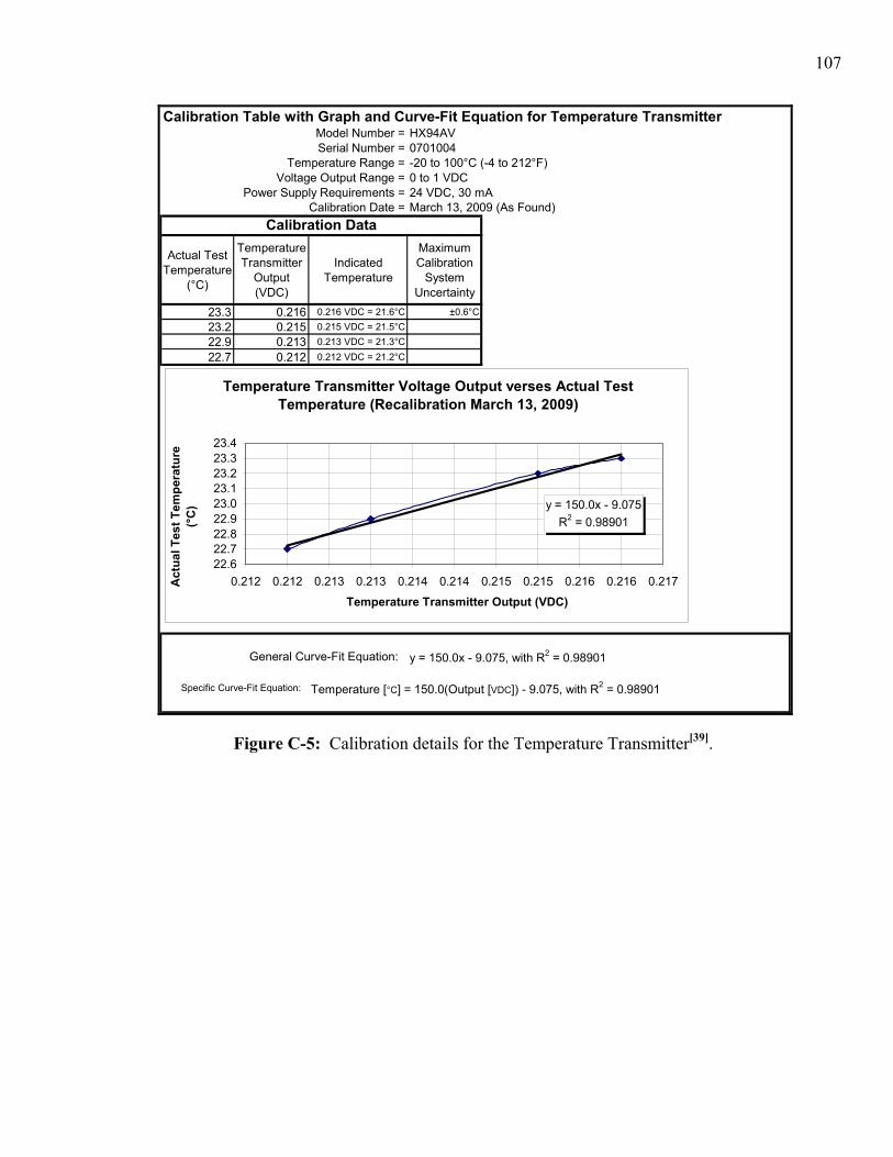
107
Actual Test Temperature
(°C)
Temperature Transmitter
Output (VDC)
Indicated Temperature
Maximum Calibration
System Uncertainty
23.3 0.216 0.216 VDC = 21.6°C ±0.6°C23.2 0.215 0.215 VDC = 21.5°C22.9 0.213 0.213 VDC = 21.3°C
22.7 0.212 0.212 VDC = 21.2°C
0701004
y = 150.0x - 9.075, with R2 = 0.98901General Curve-Fit Equation:
-20 to 100°C (-4 to 212°F)0 to 1 VDC24 VDC, 30 mA
Voltage Output Range =
Calibration Date = March 13, 2009 (As Found)
Specific Curve-Fit Equation: Temperature [°C] = 150.0(Output [VDC]) - 9.075, with R2 = 0.98901
Calibration Table with Graph and Curve-Fit Equation for Temperature TransmitterModel Number =Serial Number =
Temperature Range =
Power Supply Requirements =
Calibration Data
HX94AV
Temperature Transmitter Voltage Output verses Actual Test Temperature (Recalibration March 13, 2009)
y = 150.0x - 9.075R2 = 0.98901
22.622.722.822.923.023.123.223.323.4
0.212 0.212 0.213 0.213 0.214 0.214 0.215 0.215 0.216 0.216 0.217
Temperature Transmitter Output (VDC)
Act
ual T
est T
empe
ratu
re
(°C
)
Figure C-5: Calibration details for the Temperature Transmitter[39].

108
Actual Test Humidity (% RH)
Relative Humidity
Transmitter Output (VDC)
Indicated Humidity
Maximum Calibration
System Uncertainty
22.0 0.217 0.217 VDC = 21.7% ±2.5% RH32.9 0.341 0.341 VDC = 34.1%49.9 0.518 0.518 VDC = 51.8%
75.2 0.774 0.774 VDC = 77.4%
y = 95.90x + 0.6476, with R2 = 0.99951General Curve-Fit Equation:
3 to 95% (non-condensing)0 to 1 VDC24 VDC, 20 mA
Voltage Output Range =
Calibration Date = March 13, 2009 (As Found)
Calibration Table with Graph and Curve-Fit Equation for Relative Humidity Transmitter
Specific Curve-Fit Equation: Relative Humidity [% RH] = 95.90(Output [VDC]) + 0.6476, with R2 = 0.99951
Model Number =Serial Number =
Relative Percent Humidity Range =
Power Supply Requirements =
Calibration Data
HX94AV0701004
Relative Humidity Transmitter Voltage Output verses Actual Test Humidity (Recalibration March 13, 2009)
y = 95.90x + 0.6476R2 = 0.99951
20.0
30.0
40.0
50.0
60.0
70.0
80.0
0.200 0.300 0.400 0.500 0.600 0.700 0.800 0.900
Relative Humidity Transmitter Output (VDC)
Act
ual T
est H
umid
ity
(% R
H)
Figure C-6: Calibration details for the Relative Humidity Transmitter[39].

109
Applied Pressure (mbar)
Pressure Transducer
Output (VDC)
Nonlinearity Errors (% FS)
Extrapolated Errors (% FS)
800.0000 -0.0006 0.000 Zero -0.012900.0000 1.6673 0.015
1000.0000 3.3335 -0.003 Span 0.0271100.0000 5.0007 0.000
Calibration Table with Graph and Curve-Fit Equation for Transducer #5Model Number =Serial Number =
Pressure Range =
270
Specific Curve-Fit Equation: Pressure [mbar] = 59.987640(Output [VDC]) + 800.01740, with R2 = 0.99999996
Power Supply Requirements =
Calibration Data
Voltage Output Range =
y = 59.987640x + 800.01740, with R2 = 0.99999996General Curve-Fit Equation:
Calibration Date = May 30, 2007
3271298800 to 1100 mbar0 to 5 VDC24 VDC, 10 mA
Transducer #5 Voltage Output verses Applied Pressure
y = 59.987640x + 800.01740R2 = 0.99999996
0.0000
200.0000
400.0000
600.0000
800.0000
1000.0000
1200.0000
-0.1000 0.9400 1.9800 3.0200 4.0600 5.1000
Pressure Transducer Output (VDC)
App
lied
Pres
sure
(mba
r)
Figure C-7: Calibration details for Transducer #5[40].

110
11. APPENDIX D: WIND TUNNEL BOUNDARY-LAYER ANALYSIS
5
15 25 35 45 55 65 75 85 95
105
115
125
135
145
155
165
175
δ (ft) at x = 1 ftδ (ft) at x = 3 ftδ (ft) at x = 5 ftδ (ft) at x = 7 ftδ (ft) at x = 9 ftδ (ft) at x = 11 ftδ (ft) at x = 13 ft0.00
0.01
0.02
0.03
0.04
0.05
0.06
0.07
0.08
0.09
Bou
ndar
y-La
yer T
hick
ness
(ft)
Air Flow Velocity (mph)
Boundary-Layer Thickness for Laminar Flow
Figure D-1: Boundary-layer thickness graph for laminar flow in the UCD AWT test section using the flat plate assumption.

111
Table D-1: Boundary-layer thickness calculations for laminar flow in the AWT test section using the flat plate assumption[26].
T
able
D-1
: B
ound
ary-
laye
r thi
ckne
ss c
alcu
latio
ns fo
r lam
inar
flow
in th
e A
WT
test
sect
ion
usin
g th
e fla
t pla
te a
ssum
ptio
n[26]
.

112
5
15 25 35 45 55 65 75 85 95
105
115
125
135
145
155
165
175
δ (ft) at x = 1 ftδ (ft) at x = 3 ftδ (ft) at x = 5 ftδ (ft) at x = 7 ftδ (ft) at x = 9 ftδ (ft) at x = 11 ftδ (ft) at x = 13 ft0.00
0.05
0.10
0.15
0.20
0.25
0.30
0.35
Bou
ndar
y-La
yer T
hick
ness
(ft)
Air Flow Velocity (mph)
Boundary-Layer Thickness for Turbulent Flow
Figure D-2: Boundary-layer thickness graph for turbulent flow in the UCD AWT test section using the flat plate assumption.

113
Table D-2: Boundary-layer thickness calculations for turbulent flow in the AWT test section using the flat plate assumption[26].
T
able
D-2
: B
ound
ary-
laye
r thi
ckne
ss c
alcu
latio
ns fo
r tur
bule
nt fl
ow in
the
AW
T te
st se
ctio
n us
ing
the
flat p
late
ass
umpt
ion[2
6].

114
12. APPENDIX E: ANEMOMETER SUPPORT STRUCTURE
Figure E-1: Bridgeport three and a half axis milling machine set up to machine the slot cover for the anemometer leveling support structure (left). Close up of the slot cover partially completed on the milling machine (right).
Figure E-2: Exploded view of the “L” shaped pipe assembly (also known as the support pipe) that is composed of a 3/4 in. diameter schedule 40 galvanized steel pipe, elbow fitting, extension fitting and an anemometer female 4-pin (7 hole) connector, all of which is used in the anemometer leveling support structure.

115
Figure E-3: Top view of the following anemometer leveling support structure components that are responsible for leveling the anemometer: the pipe clamp (top left), leveling plate (top center), base plate (top right), and slot cover (bottom).
Figure E-4: Top view of the pipe clamp (top left), leveling plate (top center), and the
base plate (top right). Bottom view of the slot cover (bottom).

116
Figure E-5: Top close-up view of the pipe clamp (top left). Note that the slot on the pipe clamp (located at the bottom is this picture) will point in the direction of the air flow in the UCD AWT test section when the anemometer leveling support structure is properly installed.
Figure E-6: The fully assembled support pipe (top), and the fully assembled leveling structure (bottom) that when combined make up the anemometer leveling support structure.

117
Figure E-7: Bottom view of the anemometer leveling support structure, minus the support pipe, shown as properly installed in a slot.
Figure E-8: Top left view of the anemometer leveling support structure installed in a slot on the roof of the UCD AWT test section.

118
Figure E-9: Top view of the anemometer leveling support structure installed in a slot on the roof of the UCD AWT test section.
Figure E-10: Top close-up view focused on the base plate, leveling plate, pipe clamp, and support pipe when the anemometer leveling support structure is installed in a slot on the roof of the UCD AWT test section.

119
Figure E-11: Top close-up view (left) and top right close-up view (right) focused on the leveling plate, pipe clamp, and support pipe when the anemometer leveling support structure is installed in a slot on the roof of the UCD AWT test section.
Figure E-12: Top left close-up view (left) and top close-up view (right) focused on the leveling plate, pipe clamp, and support pipe when the anemometer leveling support structure is installed in a slot on the roof of the UCD AWT test section.

120
Figure E-13: Left side view of the anemometer leveling support structure installed in a slot on the roof of the UCD AWT test section, without an anemometer installed on the support pipe.

121
13. APPENDIX F: ANEMOMETER CALIBRATION PROGRAM
Figure F-1: Front panel of the calibration program, showing the “Real Time Data and Results” tab which displays all data and results used in anemometer calibration.

122
Figure F-2: Front panel of the calibration program, showing the “Fan Control” tab with the “Manual Fan Control” sub-tab which together display all the inputs and outputs required to successfully operate the wind tunnel fan manually.

123
Figure F-3: Front panel of the calibration program, showing the “Fan Control” tab with the “Automated Fan Control” sub-tab which together display all the inputs and outputs required to successfully operate the wind tunnel fan automatically. Note that the wind tunnel fan was operated automatically for both the anemometer and pitot-static tests.