General rights Copyright and moral rights for the publications made accessible in the public portal are retained by the authors and/or other copyright owners and it is a condition of accessing publications that users recognise and abide by the legal requirements associated with these rights.

Users may download and print one copy of any publication from the public portal for the purpose of private study or research.

You may not further distribute the material or use it for any profit-making activity or commercial gain

You may freely distribute the URL identifying the publication in the public portal If you believe that this document breaches copyright please contact us providing details, and we will remove access to the work immediately and investigate your claim.

Downloaded from orbit.dtu.dk on: Apr 06, 2022

Validation of a wind tunnel testing facility for blade surface pressure measurements

Fuglsang, P.; Antoniou, Ioannis; Sørensen, Niels N.; Aagaard Madsen, Helge

Publication date:1998

Document VersionPublisher's PDF, also known as Version of record

Link back to DTU Orbit

Citation (APA):Fuglsang, P., Antoniou, I., Sørensen, N. N., & Aagaard Madsen, H. (1998). Validation of a wind tunnel testingfacility for blade surface pressure measurements. Denmark. Forskningscenter Risoe. Risoe-R No. 981(EN)

Risø-R-981(EN)

Validation of a Wind Tunnel TestingFacility for Blade Surface PressureMeasurements

Peter Fuglsang, Ioannis Antoniou, Niels N. Sørensen,Helge Aa. Madsen

Risø National Laboratory, RoskildeApril 1998

AbstractThis report concerns development and validation of a 2d testing facility forairfoil pressure measurements. The VELUX open jet wind tunnel was usedwith a test stand inserted. Reynolds Numbers until 1.3 million were achievedwith an airfoil chord of 0.45 m. The aerodynamic load coefficients were foundfrom pressure distribution measurements and the total drag coefficient wascalculated from wake rake measurements. Stationary inflow as well as dynamicinflow through pitching motion was possible. Wind tunnel corrections wereapplied for streamline curvature and down-wash. Even though the wind tunnelis not ideal for 2d testing, the overall quality of the flow was acceptable with auniform flow field at the test stand position and a turbulence intensity of 1% atthe inlet of the test section. Reference values for free stream static and totalpressure were found upstream of the test stand. The NACA 63-215 airfoil wastested and the results were compared with measurements from FFA and NACA.The measurements agreed well except for lift coefficient values at high anglesof attack and the drag coefficient values at low angles of attack, that wereslightly high. Comparisons of the measured results with numerical predictionsfrom the XFOIL code and the EllipSys2D code showed good agreement.Measurements with the airfoil in pitching motion were carried out to study thedynamic aerodynamic coefficients. Steady inflow measurements at high anglesof attack were used to investigate the double stall phenomenon.

The Danish Energy Agency funded the present work in the contracts,ENS-1363/94-0001, ENS-1363/95-0001 and ENS-1363/97-0002.

ISBN 87-550-2300-2ISSN 0106-2840

Information Service Department, Risø, 1998

Risø-R-981(EN) 3

Contents

1 Introduction 5

2 Experimental set-up 7

2.1 The wind tunnel 72.2 The test stand 82.3 The airfoil section 102.4 The wake rake 112.5 The data acquisition system 132.6 Aerodynamic devices 14

3 Wind tunnel boundary corrections 15

3.1 Down-wash 163.2 Streamline curvature 17Method of Garner et al. 18Method of Brooks et al. 18Navier-Stokes calculation 19Comparison 213.3 Comparison and practical use 21

4 Wind tunnel flow conditions 23

4.1 Mean velocity and turbulence 244.2 Test stand vibration 264.3 Nozzle outlet flow 284.4 Tunnel centerline flow 29Velocity 29Static pressure 314.5 Test stand 32Velocity profile 32Static pressure 334.6 Wake rake 33Velocity profile 34Static pressure 34Angle of attack dependency 354.7 Wind tunnel reference 37

5 Calculation methods 38

5.1 Density, pressures and velocity 385.2 Airfoil forces from pressure distribution 395.3 Airfoil drag from wake rake 40

Risø-R-981(EN)4

6 Results 41

6.1 Pressure distributions 416.2 Polar results 46Lift coefficient 46Drag coefficient 48Moment coefficient 506.3 Leading edge roughness 51Pressure distributions 51Polar results 526.4 Dynamic stall 54Dynamic hysteresis loops 56Reduced frequency k = 0.044 57Reduced frequency k = 0.022 626.5 Double stall 67Area 1 70Area 2 71Area 3 72

7 Conclusions 74

References 76

A1 Measurement survey 76

A1.1 Measurement types 76A1.2 Data file naming convention 77A1.3 Data file format 78A1.4 Performed measurements 79

Risø-R-981(EN) 5

1 Introduction

The development of modern airfoils for use on wind turbines was initiated inthe 1980’s. The requirements for such airfoils differ from standard aviationairfoils, because of structural reasons and extensive aerodynamic off-designoperation conditions. Wind turbine airfoils operate frequently under fullyseparated flow when stall is used for power regulation at high wind speeds.Even in the case where traditional aviation airfoils are used on wind turbines,their performance needs to be verified in the entire operational range and atsuitable Reynolds numbers. Eventually these airfoils are modified for improvedperformance by aerodynamic devices, such as vortex generators and gurneyflaps. Thus there is a need for continuos testing of new airfoil configurations.

Modern airfoils are to a large extent developed from numerical calculations andoptimization studies. Flow conditions such as separation at high angles ofattack, laminar separation bubbles and transition from laminar to turbulent floware difficult to predict accurately. Hence, testing of airfoils is an importantissue in airfoil design. Tests of subsonic airfoils for wind turbines are carriedout by a number of different research institutes, among these NationalRenewable Energy Laboratory, NREL, USA [2], Delft University, NL [3] FFA,S [4] and The University of Southampton, UK [6]. Such tests demand theavailability of suitable wind tunnels that are often available from the generalaviation industry and research. So far, testing of airfoils under typical windturbine operation conditions was not possible in Denmark and was insteadcarried out by foreign cooperation partners, such as [4], [5] and [6].

In the autumn of 1993, a newly build wind tunnel became available inDenmark. The tunnel is of the closed return type with a 3.4x3.4 m open jetblowing into a test section with a cross section of 7.5x7.5 m, which is 10.5 mlong. The tunnel was in 1994 used for 3d tests of a full-scale non-rotating LM8.2 blade [14]. These tests show promising results, and confirm that the flowquality allows the use of the tunnel for tests of 2d airfoil sections, though it isobvious, that the tunnel test section is not ideal for obtaining 2d flows.

This report presents the developed facility for the experimental testing of 2dairfoil sections for use on wind turbine blades. The aim is to document thetesting facility by reporting both static and dynamic pressure distributionmeasurements for the well known, NACA 63-215 airfoil [1]. The measurementsinclude static and dynamic measurements up to angles of attack around 30°.The airfoil section was mounted horizontally in a test stand with endplates toensure 2d flow conditions. The flow was free to expand in the verticaldirection, but bound by the test section floor at a distance of 3.5 chords belowthe airfoil.

Risø-R-981(EN)6

Overall requirements to the test method were:• To become able to carry out both static measurements and dynamic

measurements with the airfoil in pitching motion.• To allow testing of Reynolds numbers until 1.5×106, achieved by a flow

velocity of 40 m/s and airfoil chord up to 0.60 m.• To limit the period from airfoil design to airfoil test, involving molding of

the airfoil section, mounting of the pressure tubes, testing and evaluation ofresults.

• To accomplish a cost effective testing by intensive use of the tunnel time,which is rented on an hourly basis. The intensive use of the tunnel is alsodictated from geographic reasons, since the tunnel is located away fromRisø.

The report was structured in the following chapters:

Chapter 2 describes the experimental setup, the wind tunnel and the dataacquisition system.

Chapter 3 describes the implementation of wind tunnel corrections to measuredraw data.

Chapter 4 evaluates the wind tunnel flow conditions for calibration of staticpressure and velocity and a proper wind tunnel reference is established for thenon-dimensional reporting of airfoil aerodynamic forces.

Chapter 5 describes the methods used to calculate velocities, pressures andairfoil lift, drag and moment coefficients, including the total drag coefficientfrom the wake rake.

Chapter 6 contains the measured static and dynamic results together with ananalysis of ‘double stall’ measurements.

Chapter 7 is the report conclusions

Appendix 1 is a more detailed description of the performed measurements foruse in future exploitation of the results.

Risø-R-981(EN) 7

2 Experimental set-up

The present chapter describes the experimental setup. The description includesthe wind tunnel test section, the test stand, the airfoil section, the wake rake andthe data acquisition system.

2.1 The wind tunnelThe VELUX wind tunnel is of the closed return type with a practically opentest section. The test section has a cross section of 7.5x7.5 m and a length of10.5 m and the dimensions of the ‘active’ test section are determined by a jetnozzle of adjustable dimensions (maximum 4.0x4.0 m, minimum 3.4x.3.4 m).For the needs of the present tests the small jet nozzle of 3.4x3.4 m is used. Thejet nozzle protrudes 1.75 m into the test section and blows the air towards theexit, which is a nozzle of dimensions 4.0x4.0 m. The maximum flow velocityachieved in the tunnel depends on the nozzle dimensions and when the smallnozzle is used the maximum velocity is around 45 m/s. A perspective drawingof the tunnel test section is shown in Figure 2-1. In Figure 2-2 and Figure 2-3the tunnel test section is shown with the test stand installed from different viewangles, in order to give the reader a feeling of the tunnel’s size relative to thetest stand and the airfoil section. The test section floor is equipped with aturntable of 2 m in diameter on which the test stand is fastened. The test standand the airfoil section are assumed perpendicular to the tunnel flow once theleading edge of the airfoil section is adjusted parallel to the nozzle exit.

10.50

7.504.00

3.40

2.50

1.702.651.75

4.00

Turn table

Figure 2-1 A schematic drawing of the wind tunnel test section with the teststand.

Risø-R-981(EN)8

Figure 2-2 The test section when looking upwind. The adjustable jet nozzle canbe seen behind the test stand

Figure 2-3 The test section when looking downwind.

2.2 The test standThe tunnel in itself is not well suited for 2d airfoil section testing, and a teststand was built for that purpose. It consists of three metal U-profiles assembledtogether to form an inverse Π. To reduce flow disturbances, the stand is given asmooth aerodynamic shape, achieved by the use of ferrying surfaces with gentleslopes around the metal profiles. Airfoil sections of approximately 1.9 m width,mounted approximately at 1.7 m from the tunnel floor and 2.8 m from thenozzle inlet, can be tested with this stand. The airfoil section used in the presenttests has a chord of 0.45 m, which means that the aspect ration of the airfoilsection is 4.25.

The airfoil section must either span the width of the test section or be confinedbetween vertical walls placed inside the tunnel. In the absence of end walls 3dflow effects will occur. A consequence of this would be a non-uniformdistribution of the circulation along the airfoil and because of this a non-uniform distribution of the angle of attack. To avoid end effects in the presenttests, endplates are used. The endplates are fixed to the test stand and do not

Risø-R-981(EN) 9

turn with the angle of attack. The endplates have to be placed as close to theairfoil as possible, to limit 3d effects. At the same time they should not come incontact with the airfoil and influence its motion during operation. In order tominimize the clearance between the endplates and the airfoil section, thehorizontal position of the endplates is adjustable by a few millimeters with thehelp of a set of bolts. The combination of these adjustments with the use offillers between the airfoil and the endplates during mounting ensures that theclearance during operation does not exceed one millimeter in the worst case. Toallow quick interchange of airfoils during the tests each endplate is split into anupper and a lower part.

Lineartranslationmotor

Pitching motionmechanism

Control systemand

asynchronousmotor

Slide rule

Gear box

Figure 2-4 The mechanism that allows static and dynamic measurements to bemade.

Figure 2-4 shows the instruments embedded to the side of the test stand. Bothstatic and dynamic measurements are possible with this stand. Static testscomprise measurements at different angles of attack that can be adjustedcontinuously. They take place with the help of a linear translation motor thatmoves a steel rod in the vertical direction. The dynamic measurements involvepitching of the airfoil section at different amplitudes and different reducedfrequencies. A pitching motion mechanism, driven by an asynchronous motor,can pitch the airfoil section at pre-defined amplitudes and frequencies. This isachieved by introducing a perforated circular plate between the steel rod and

Risø-R-981(EN)10

the gearbox. The plate has holes at different radial positions that correspond toamplitudes from 2° to 5°. Different amplitudes can be achieved by selecting theproper radial distance. A control and feed back electronic system together witha suitable gearbox (gear ratio) makes possible a wide range of reducedfrequencies. If different frequencies are wanted then the gearbox isinterchanged. The pitching mechanism is suspended from the linear translationmotor, which slides the mechanism in the vertical direction. Thereby it is usedto control the angle of attack during static tests. To achieve a continuous slowpitching of the blade, a regulating power supply unit is used.

2.3 The airfoil sectionThe airfoil section model tested is the NACA 63-215. The span of the model is1.9 m and the chord is 0.45 m. Originally it was manufactured and tested byFFA in a Danish funded project [4]. FFA borrowed the model to Risø andprovided both the airfoil cross section coordinates and the locations of the taps.

The airfoil section is equipped with 64 pressure taps. Of these taps 57 aresituated along the chord at the centerline. The location of the pressure tabs canbe seen in Figure 2-5 where the FFA model is compared with the theoreticalcoordinates from [1]. The distribution of the tubes in the chordwise direction isnon uniform, with more tubes situated around the leading edge where the flowis accelerated. The overall agreement between the actual FFA model and thetheoretical coordinates is good in the leading edge region. However at thetrailing edge, due to manufacturing reasons, the FFA model thickness isincreased compared to the theoretical coordinates.

0

0.2

0 0.2 0.4 0.6 0.8 1

y/c

x/c

NACA 63-215 FFA ModelNACA 63-215 Coordinates from [1]

-0.05

-0.025

0

0.025

0.05

0 0.02 0.04

y/c

x/c

-0.025

0

0.025

0.05

0.75 0.8 0.85 0.9 0.95 1

y/c

x/c

Figure 2-5 NACA 63-215 airfoil section where each symbol is a pressure tab.The FFA model is compared with the theoretical coordinates from [1]. Theleading edge and the trailing edge regions are shown enlarged.

Risø-R-981(EN) 11

Holes are drilled on the surface and metal tubes are fitted to the holes andmounted flash with the surface. Flexible plastic tubes are mounted at the endsof the metal tubes. The tubes exit assembled from the airfoil section through ahollow suspension axis, Figure 2-6. To minimize flow disturbances, which mayinfluence the flow and lead to premature transition, the holes are in a staggeredarrangement along the span of the airfoil section.

Figure 2-6 The pneumatic plastic tubes exit from the suspension axis of theairfoil section.

The airfoil section is suspended on two vertical metal profiles of the test standby two metal axis fitted on two bearings, Figure 2-6 and Figure 2-7. A winddirection resolver is fastened on the opposite side axis to measure the changesof the angle of attack, Figure 2-7.

Figure 2-7 The wind direction resolver used for measurement of the airfoilsection angle of attack.

2.4 The wake rakeThe wake rake can be seen in Figure 2-8 and Figure 2-9. It consists of 54 totalpressure probes of 1 mm inner diameter and five 4 mm inner diameter statictubes. The span width covered by the static tubes is 0.456 m. The distribution

Risø-R-981(EN)12

of the total pressure tubes in the rake is non uniform and towards the middle ofthe rake, see Figure 2-9, the tube spacing is more dense compared to the rakeends. The five static tubes are spaced equidistant.

Figure 2-8 The wake rake behind the test stand.

Figure 2-9 The wake rake seen from the side.

The rake is rigidly mounted on a metal mast behind the airfoil section, Figure2-9. The metal mast is fastened both to the test stand and on a rectangular baseby four supporting wires to avoid vibrations due to excitation of theconstruction. During the tests the distance from the head of the static tubes tothe airfoil section trailing edge is 0.7 chords and the middle of the wake rake isplaced at the height of the trailing edge at 0° inclination. The rake cannot betraversed in either the horizontal or the vertical direction. Hence, its center doesnot follow the translation of the minimum of the pressure deficit due to thechange in the angle of attack and the streamline curvature. At higher angles ofattack the deficit is not as accurately described as in the case of the smallerangles due to the larger distance between the total pressure holes. Anotherreason for the failure of the wake rake at higher angles of attack is that the flowaround the airfoil separates and becomes highly unstable and the measuredwake drag cannot be considered as representative of the airfoil drag.

Risø-R-981(EN) 13

The measurement of both the total and static pressures takes place by using a10´´ H20 pressure module. When the static pressure is needed between the staticpressure tubes at the location of the corresponding total pressure holes, thestatic pressure is found by linear interpolation.

2.5 The data acquisition systemThe data acquisition system used in the present tests is the HyScan 2000 systemof Scanivalve Corp. It is a combination of both hardware and software andconsists of two ZOC33 pressure-scanning modules used to record the pressuresignals and a ZOCEIM16 module used for the rest of the electrical signals.

The ZOC33 consists of an electronic pressure scanner that accepts 64pneumatic inputs that are directed to 64 silicon pressure sensors. The sensorsconvert the pressure signals to electrical output that can be read by a computer.Each module is equipped with a calibration valve, a high speed (50 kHz)multiplexer and an instrumentation amplifier. By multiplexing the inputs of thethree modules, the total sampling speed can thus reach 100 kHz. The pressuresensors are collected in groups of eight, which allows incorporation of variouspressure ranges within the same module.

The calibration valve can be operated in four different modes:• operate• calibrate• purge• leak test.

Applying the appropriate pneumatic control activates these modes. As a resultthe pressure modules can be calibrated/checked during a measurement session.The architecture of the pressure scanner is seen in Figure 2-10. As the siliconpressure sensors are known to be temperature dependent, the modules areplaced inside thermal control units (TCU). The TCU is designed to provide aconstant temperature environment for the pressure scanners while beingequipped with electrical and pneumatic connections, thus functioning as anintermediate between the ZOC and the rest of the system.

Figure 2-10 The architecture of the pressure module.

In the present tests the module used to record the blade pressures consists of 401 psi and 24 2.5 psi sensors. The latter ones are used to record the pressures

Risø-R-981(EN)14

around the leading edge. The module used for the measurement of the wakerake pressures is a 10´´ H20.

Besides the ZOC modules, the HyScan 2000 system comprises the following:• The IFM 2000 ZOC module, interface to the module units containing line

drivers and addressing circuitry.• The CSM 2000 unit (cable service module) used to service the ZOC

modules. It can support up to eight ZOC modules. Its function is to providethe modules with DC power. It receives address information from the IFM2000 and sends the analogue signals from the ZOC modules to theIFM2000.

• The CPM 3000 (control pressure module) which contains the valvesnecessary to switch the ZOC calibration valves in one four modes ofoperation.

• The SPC 3000 (secondary pressure standard) which is used to calibrate thepressure modules since it can provide known calibration pressures.

• A data acquisition board plugged inside the computer, which can sample upto 100 kHz.

At normal operation, a total of 134 signals are measured by the data acquisitionsystem:

• 64 Airfoil surface static pressures• 5 wake rake static pressures• 53 wake rake total pressures• 3 Pitot tube static pressures• 3 Pitot tube total pressures• Angle of attack• Air temperature• Air density• 2 strain gauges for recording shaft bending• Electric motor frequency

The latter six signals are those sampled via the ZOEIM16.

2.6 Aerodynamic devicesIn some of the measurements, leading edge roughness was simulated bysandpaper mounted on the airfoil suction side from the leading edge to 5%chord. The type NAXOS, grain size 120, width 32 mm was used. Leading edgeroughness was not applied to the pressure side.

Risø-R-981(EN) 15

3 Wind tunnel boundary corrections

The flow conditions in the wind tunnel test section are not the same as those infree flow. Both closed jet as well as open jet boundaries produces extraneousforces, that must be taken into account. Additionally a longitudinal staticpressure gradient is also present in the test section. There is a large amount ofliterature available on closed jets and ventilated wall wind tunnels, as, e.g., [7].However, open jet test sections are rarely used for 2d testing, and only a fewreferences were available to the present study, [6 - 8], [15].

Because the cross section of the test section is larger than the inlet nozzle crosssection, the jet flow is free to expand and the tunnel is an open jet tunnel. Sincethe airfoil section does not span the width of the jet, endplates have to bemounted to the ends of the airfoil section to approximate 2d flow. The smallclearances between the airfoil section and the endplates, the finite size of theendplates and the presence of the floor and the ceiling introduce uncertaintieson the wind tunnel corrections.

The wind tunnel corrections do not take into account additional effects fromcustomary failings of the wind tunnel, such as non-horizontal flow in the testsection, local variations in velocity and pressure and interference anddisturbances. The variation in velocity and pressure will be dealt with inchapter 4. The remaining effects are assumed to be negligible.

The following wind tunnel corrections were considered:

• Solid and wake blockage• Horizontal buoyancy• Down-wash• Streamline curvature

Solid and wake blockages are constraints to the flow pattern that increase withwake size and blocking of the tunnel cross section. These are important for aclosed jet tunnel, but are usually negligible for open jet flows, since the flow isfree to expand [7].

In the case of tunnels with closed test sections horizontal buoyancy results fromthe thickening of the boundary layer as it develops in the downstream directionwithin the test section. The free flow area is reduced, the flow accelerates andas a result the density of the streamlines is increased and there is a drop in thestatic pressure along the test section. This pressure-drop results in a drag forceon the airfoil section. In the case of tunnels with open test sections, the pressuredrop is very limited and so is the influence of horizontal buoyancy [7].

For an open jet flow, the remaining two corrections, down-wash and streamlinecurvature, are significant and they are explained in the following. Thesecorrections are applied directly on the lift coefficient, CL, the drag coefficient,CD and the moment coefficient, CM, but not on the airfoil pressure distribution.

Risø-R-981(EN)16

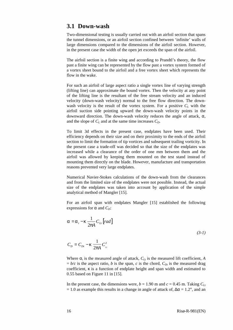
3.1 Down-washTwo-dimensional testing is usually carried out with an airfoil section that spansthe tunnel dimensions, or an airfoil section confined between ‘infinite’ walls oflarge dimensions compared to the dimensions of the airfoil section. However,in the present case the width of the open jet exceeds the span of the airfoil.

The airfoil section is a finite wing and according to Prandtl’s theory, the flowpast a finite wing can be represented by the flow past a vortex system formed ofa vortex sheet bound to the airfoil and a free vortex sheet which represents theflow in the wake.

For such an airfoil of large aspect ratio a single vortex line of varying strength(lifting line) can approximate the bound vortex. Then the velocity at any pointof the lifting line is the resultant of the free stream velocity and an inducedvelocity (down-wash velocity) normal to the free flow direction. The down-wash velocity is the result of the vortex system. For a positive CL with theairfoil suction side pointing upward the down-wash velocity points in thedownward direction. The down-wash velocity reduces the angle of attack, α,and the slope of CL and at the same time increases CD.

To limit 3d effects in the present case, endplates have been used. Theirefficiency depends on their size and on their proximity to the ends of the airfoilsection to limit the formation of tip vortices and subsequent trailing vorticity. Inthe present case a trade-off was decided so that the size of the endplates wasincreased while a clearance of the order of one mm between them and theairfoil was allowed by keeping them mounted on the test stand instead ofmounting them directly on the blade. However, manufacture and transportationreasons prevented very large endplates.

Numerical Navier-Stokes calculations of the down-wash from the clearancesand from the limited size of the endplates were not possible. Instead, the actualsize of the endplates was taken into account by application of the simpleanalytical method of Mangler [15].

For an airfoil span with endplates Mangler [15] established the followingexpressions for α and CD:

[ ]radCA Ltt π

καα2

1−=

(3-1)

C CA

CD Dt Lt= − κ

π1

22

Where αt is the measured angle of attack, CLt is the measured lift coefficient, A= b/c is the aspect ratio, b is the span, c is the chord, CDt is the measured dragcoefficient, κ is a function of endplate height and span width and estimated to0.55 based on Figure 11 in [15].

In the present case, the dimensions were, b = 1.90 m and c = 0.45 m. Taking CLt

= 1.0 as example this results in a change in angle of attack of, ∆α = 1.2°, and an

Risø-R-981(EN) 17

induced drag of, ∆CD = -0.021. Compared to an airfoil section withoutendplates, down-wash was reduced by 45%.

3.2 Streamline curvatureStreamline curvature is introduced to the jet flow when the flow is free todiverge from its original direction downstream of the airfoil section. In openjets, this effect is usually large because the tunnel walls do not bound the jetflow. The curvature of the tunnel flow induces both drag and changes of theeffective angle of attack. As a result the measured CD is too large and the slopeof the CL curve is too small.

In the following, the results of two analytical correction methods from Garneret al. [8] and Brooks et al. [9] are compared to results of numerical Navier-Stokes calculations of the flow field. It is assumed that in this flow field theairfoil is placed in an open jet flow with open top and bottom boundaries. Solidwalls or large endplates are present to preserve the two-dimensionality of theflow. It is also assumed that the airfoil is placed in the middle of the open jet ath/2, where h is the jet height.

Both analytical methods use the method of images where the airfoil is replacedeither by a single vortex or a distribution of vortices along the chord and theflow field is approximated by a series of image vortices with respect to thevertical dimensions of the jet. Figure 3-1 shows the model of the 2d tunnelflow, where the airfoil chord, c, the upstream distance to the nozzle, d, and hare the important dimensions. The airfoil is replaced by a single vortex whilethe flow is approximated by the image system seen in Figure 3-1. Thiscorresponds to a cascade flow.

Figure 3-1 Airfoil and image system employed for derivation of 2d open jetwind tunnel correction (ref. [9]).

Risø-R-981(EN)18

Method of Garner et al.

The method of Garner et al. [8] is first order accurate. A balance of momentumis used together with the vortex image system. The results are obtained by usinga flat plate of chord, c, placed midway between the boundaries of the simulatedopen test section of a wind tunnel and at an angle of, αt = 10°. To simulate thecirculation around the plate, a single vortex at x = ¼ c is used. It is assumed,that the interference down-wash at the plate is half that in the distant wake.

The free flow angle of attack, α, is found from:

(3-2)

Where CLt is the measured lift coefficient and αt is the measured angle of attack.The 2d lift divided by the total lift, L0 /L, is found from Figure 3-2. (c/h =0.4/3.4 ≈ 0.11 ⇒ L/L0 ≈ 0.88).

The free flow drag, CD, is found from:

(3-3)

Where CDt is the measured drag.

Figure 3-2 L/L0 shown as function of chord to tunnel height ratio, c/h (ref. [8]).

Method of Brooks et al.

The method of Brooks et al. [9] is of higher order accuracy compared to Garneret al. [8]. It involves additional terms on the correction of the angle of attackand a correction of the moment coefficient. Compared to Garner et al. [8], thecirculation around the airfoil is not replaced by a single vortex, but by vorticesdistributed along the airfoil chord.

[ ]radCL

LLt

ot

−−= 1

2

1

παα

212

1Lt

oDtD C

L

LCC

−−=

π

Risø-R-981(EN) 19

The free flow moment coefficient, CM, is obtained:

(3-4)

Where CMt is the measured moment coefficient, CLt is the measured liftcoefficient and σ is defined as:

22

48

⋅=

h

cπσ

(3-5)

The free flow angle of attack, α, is found from:

(3-6)

The drag, CD, is calculated from the correction due to the induced down-wash:

(3-7)

Where CDt is the measured drag coefficient.

Navier-Stokes calculation

To confirm the results of the analytical methods, Navier-Stokes calculationswere performed with the EllipSys2D code [12] on a cascade type flow, similarto the arrangement shown in Figure 3-1. The chord was in this case, c = 0.60and the jet height, h = 3.4. The airfoil was the NACA 63-215 airfoil.

The cascade flow was compared to 2d free flow calculations to reveal thedifference in α and CD for equal CL. Figure 3-3 shows the CL curve for the freeflow and for the cascade flow. The CL curve slope was clearly lower for thecascade flow due to a change in angle of attack. A correction to the cascadeflow was applied on basis of eq. (3-2) by adjusting the cascade flow angle ofattack so that the corrected cascade flow CL was in agreement with CL at 8o forthe free flow:

(3-8)

Where α and αt are given in degrees.

It appears from the corrected cascade flow CL curve in Figure 3-3, that there isgood agreement between the corrected cascade flow CL curve and the free flowCL. This is further supported by comparing the pressure distributions for thefree flow at α = 7.5o with results from the cascade flow at α = 10.0o shown inFigure 3-4. It can be seen that the two pressure distributions coincide, whichconfirms the results of the lift distribution and the validity of the analyticalcalculation.

LtMtM CCC2

σ−=

( )[ ]radCCC MtLtLtt 423

πσ

πσ

πσαα −−−=

LtLtDtD CCCC

−+=

πσ3

Ltt C⋅−= 7.2αα

Risø-R-981(EN)20

0

0.2

0.4

0.6

0.8

1

1.2

1.4

0 5 10 15 20

CL

α

2-d free flow2-d cascade flow

corrected cascade flow

Figure 3-3 Calculated CL curves for 2d free flow and 2d cascade flowcompared to corrected cascade flow, EllipSys2D, NACA 63-215, Re = 1.3×106.

-4

-3

-2

-1

0

10 0.2 0.4 0.6 0.8 1

CP

x/c

2-d free flow, α = 7.5o

2-d cascade flow, α = 10.0o

Figure 3-4 Calculated CP curves for 2d free flow at 7.5° compared with 2dcascade flow at 10.0°, EllipSys2D, NACA 63-215, Re = 1.3×106.

The difference in CD is shown in Figure 3-5. A correction to the cascade flowwas applied on basis of eq. (3-3) by adjusting the induced drag so that thecorrected cascade flow CD was in agreement with CD at 8o for the free flow:

(3-9)

The corrected cascade flow CD is seen to fit the free flow CD well.

2045.0 LtDtD CCC ⋅−=

Risø-R-981(EN) 21

0

0.02

0.04

0.06

0.08

0.1

0.12

0.14

0 5 10 15 20

CD

α

2-d free flow2-d cascade flow

corrected cascade flow

Figure 3-5 Calculated CD curves for 2d free flow and 2d cascade flowcompared to corrected cascade flow, EllipSys2D, NACA 63-215, Re = 1.3×106.

Comparison

The Navier-Stokes calculations have been compared with the results of twoanalytical methods. The dimensions are in this case, c = 0.45 and h = 3.4corresponding to the wind tunnel and the actual airfoil section. The threemethods are compared in Table 3-1 with CLt = 1.0 and CMt = 0.0. CM is of minorimportance to the correction.

We find L/L0 = 0.82 in Figure 3-2 and σ = 3.6⋅10-3 from eq. (3-3). The resultingcorrections are in very good agreement and either of the methods can bechosen. In the following the method of Brooks et al. [9] is applied.

Table 3-1 Comparison of the different analytic correction methods from [8]and [9] with Navier-Stokes calculations at c = 0.45m, h = 3.4m, CL = 1.0.

∆∆αα (o) ∆∆CD ∆∆CM

Method of Garner et al. [8] -2.00 -0.036 -

Method of Brooks et al. [9] -2.04 -0.033 0.0018

CFD Calculations -2.0 -0.03 -

3.3 Comparison and practical useBoth down-wash and streamline curvature result in a change in the angle ofattack due to the appearance of an induced velocity normal to the flow directionand the airfoil section.

The combination of corrections for down-wash and streamline curvature isproblematic. Because of different assumptions the corrections can not directly

Risø-R-981(EN)22

be combined. Comparing the example calculation in Chapter 3.1 with Table 3-1it can be seen that streamline curvature is more important than down-wash.

The streamline curvature correction assumes 2d flow with absent boundaries inthe vertical direction, where the flow is free to expand. The floor is near to thejet in the present case and this will reduce the deviation of the flow. It istherefore chosen to apply the streamline curvature correction of Brooks et al.[9] and to neglect down-wash. The results in Chapter 6 support the validity ofthis.

Risø-R-981(EN) 23

4 Wind tunnel flow conditions

This chapter concerns measurements of the wind tunnel flow conditions. Weinvestigate the quality of the undisturbed flow and establish the proper tunnelreference velocity and static pressure at the test stand. The wind tunnelreference is important for the proper normalization of the aerodynamic forces.Possible reference measurement positions are the Pitot tubes 1-3, see Figure4-1. Pitot 1 and 2 are located near to the nozzle outlet at airfoil section heightwhereas Pitot 3 is placed above the wake rake. The reference measurementsshould be independent of the airfoil section flow field.

10.50

7.504.00

3.40

4.00

.50

.50

.75

.75

2.651.75

Pitot 2

Pitot 1Pitot 3

Pitot 1

.85

Airfoil section

Wake rake

Figure 4-1 Sketch of the wind tunnel with Pitot 1-3 together with the test standwith the airfoil section and the wake rake behind the airfoil section.

To overall evaluate the quality of the flow field, the following investigationswere carried out:• To determine the mean velocity and the turbulence intensity at different

locations long time series were measured at the different Pitot tubepositions.

• To investigate the vibration of the test stand from the interaction with theflow field long time series were measured at the test stand with the airfoilsection present.

• To determine the uniformity of the flow field at the nozzle outlet,measurements were taken on a line perpendicular to the flow direction atthe airfoil section height.

• To take into account speed up effects and the static pressure loss, thedevelopment of the flow downstream towards the test stand was measuredat several positions between the nozzle outlet and the test stand.

• To investigate the uniformity of the flow at the airfoil section, the flow atthe test stand was measured in the cross-flow plane in the downstreamdirection at the airfoil section position in the test stand.

Risø-R-981(EN)24

• To calculate total drag and to investigate the uniformity of the flow field atthe wake rake, possible disturbances from the test stand and the blockingfrom the airfoil section wake rake measurements were taken with andwithout the airfoil section.

• Based on the different measurements reference values for velocity andstatic pressure were found from the pitot tubes 1-3.

The measurements refer to the coordinate system defined in Figure 4-2. Theorigin is on the centerline of the airfoil section at the position of the shaft,which is at 40% chord. The positive x-axis direction is downstream and thepositive z-axis is toward the tunnel ceiling.

All measurements were taken at flow velocities of around 40 m/s. The resultswere compiled from different measurement runs and there were smalldifferences in the velocities due to the starting and stopping of the wind tunneland to the change in temperature. All measurements were corrected to standardtemperature and pressure conditions. To be able to compare measurementsfrom different runs, the measured velocities were given relative to the Pitot 1velocity. Correspondingly, the static pressures were shown as the differentialpressure relative to Pitot 1. Each measurement is explained in Appendix A1.

4.1 Mean velocity and turbulenceTo determine the mean velocity and the turbulence intensity at differentlocations long time series were measured at the Pitot tube positions.

Figure 4-3 shows a part of a time series of the velocity at the Pitot 1 positionfrom a 180 s record, sampled at 100 Hz. The airfoil section was mounted on thetest stand. The mean velocity and turbulence intensity were found at differenttunnel locations, Table 4-1. The turbulence intensity at the inlet was 1.0%. Thiswas increased to 1.1% downstream at the Pitot 3 position. Comparisons ofmeasurements with and without the airfoil section present showed that theturbulence intensity was not affected by its presence, Table 4-1.

x

y

z

Figure 4-2 Coordinate system definition for the flow measurements in thischapter.

Risø-R-981(EN) 25

38.5

39

39.5

40

40.5

41

0 2 4 6 8 10

v pit

ot1

t

Figure 4-3 The velocity measured by Pitot 1 with the airfoil section mounted.Part of a time series from a 180 s record (NA63215STAT221196V1).

The Pitot tubes can not resolve the presence of high frequencies correctlybecause the pressures are measured through long tubes. Figure 4-4 shows thePSD spectrum corresponding to the time series in Figure 4-3.

0

0.005

0.01

0.015

0.02

0.025

0.03

0.035

0.04

0.045

0.05

0 2 4 6 8 10

PSD

f

Figure 4-4 PSD spectrum of a velocity time series measured by Pitot 1 shownin Figure 4-3 (NA63215STAT221196V1).

Table 4-1 Mean velocity and turbulence intensity at different wind tunnellocations. Values in brackets correspond to measurements without the airfoilsection mounted. (NA63215STAT221196V2)

Velocity (m/s) Velocity relative toPitot 1

Turbulence intensity,I, (%)

Pitot 1 39.65 - 1.0Pitot 2 40.00 1.0088 0.85Pitot 3 42.18 1.064 1.1 (1.2)Wake rake 41.75 1.053 0.77 (0.73)

Risø-R-981(EN)26

There was a peak of energy at 3.4 Hz. This peak was also found for Pitot 2. Itcould not be determined whether this peak came from the jet itself, the inletgeometry or from vibrations of the Pitot stands. We did not find peaks at higherfrequencies.

Figure 4-5 shows the PSD spectrum for a velocity time series from a 180 srecord measured by Pitot 3. The 3.4 Hz peak was present, but was reduced inmagnitude, while a harmonic at 6.6 Hz appeared.

0

0.05

0.1

0.15

0.2

0.25

0.3

0.35

0.4

0 2 4 6 8 10

PSD

f

Figure 4-5 PSD spectrum of a velocity time series from a 180 s recordmeasured by Pitot 3 (NA63215STAT221196V1).

4.2 Test stand vibrationTo investigate the he vibration of the test stand from the interaction with theflow field long time series were measured at the test stand with the airfoilsection present. Time series of the angle of attack, α, and the correspondingcalculated lift coefficient, CL, were analyzed.

Figure 4-6 shows a part of a 30 s long time series, sampled at 100 Hz. Theangle of attack around α = 12.8o and was not changed.

Risø-R-981(EN) 27

12.2

12.4

12.6

12.8

13

13.2

13.4

0 2 4 6 8 10

α

t

Figure 4-6 Part of a 30 s long time series, sampled with 100 Hz, of the angle ofattack with the airfoil section mounted (NA63215STAT221196V1).

The corresponding PSD spectrum is shown in Figure 4-7. There were frequencypeaks at 3.4, 6.6, 7.8, 13.9 and 15 Hz. The peaks at 3.4 and 6.6 Hz were alsopresent in the flow, Figure 4-4 and Figure 4-5, whereas the higher frequenciesoriginated from resonance from the test stand itself or from noise.

0

0.001

0.002

0.003

0.004

0.005

0.006

0.007

0.008

0.009

0 5 10 15 20

PSD

f

Figure 4-7 PSD spectrum of the angle of attack time series from Figure 4-6.

Figure 4-8 shows the PSD of CL corresponding to the time series of α in Figure4-6. The peak at 6.6 Hz was also present in the flow. Except for lowfrequencies there were no significant frequency peaks.

Risø-R-981(EN)28

0

5e-005

0.0001

0.00015

0.0002

0.00025

0.0003

0.00035

0.0004

0.00045

0.0005

0 2 4 6 8 10

PSD

f

Figure 4-8 PSD spectrum of the CL time series corresponding to the angle ofattack from Figure 4-6.

From both Figure 4-7 and Figure 4-8, it is obvious that the energy contents ofthe spectra were limited and there were no severe resonance related to the teststand and the airfoil static pressure distribution measurements.

4.3 Nozzle outlet flowTo determine the uniformity of the flow field at the nozzle outlet,measurements were taken on a line perpendicular to the flow direction at theairfoil section height without the presence of the airfoil section.

Figure 4-9 shows the horizontal velocity profile at the inlet at the airfoil sectionheight where, z = 0.

Only three measurement points were available. The velocity profile presented aminimum at the tunnel centerline, while it was increased away from the

0.985

0.99

0.995

1

1.005

1.01

1.015

-0.6 -0.4 -0.2 0 0.2 0.4 0.6

v/v p

itot

1

y

Figure 4-9 The horizontal velocity profile at the inlet at x = -3.00 m, z = 0.0.

Risø-R-981(EN) 29

centerline toward the nozzle walls. The velocity profile was asymmetric andhigher velocities were observed towards negative y-values. This was caused bythe jet inlet geometry, where the flow was bend before the jet inlet.

The velocity can be expected to increase towards the nozzle walls because ofthe contraction of the jet. This is also found at lower velocities in earlierinvestigations by VELUX [10] and Risø [11]. The latter based on both Navier-Stokes calculations and measurements in the tunnel. The overall differencebetween the velocities was however small.

The velocity profile at the nozzle outlet vertical centerline can be seen in Figure4-10, Section 4.4. At the inlet where, x = -3.0, the flow was accelerated towardthe tunnel floor because of the jet contraction. The minimum velocity wasobserved at the airfoil section height at z = 0. Above z = 0 the velocity wasagain increased. Even though the horizontal centerline of the jet was located atz = 0.3, and minimum velocity could be expected here, the minimum velocityappears at z = 0.0 This was reproduced in several measurements. The variationwas small and of minor importance.

4.4 Tunnel centerline flowTo take into account speed up effects and the static pressure loss, thedevelopment of the flow downstream towards the test stand was measured atseveral positions between the nozzle outlet and the test stand. Together with thePitot tube measurements, this enables the establishment of the wind tunnelreference for velocity and static pressure.

Velocity

The vertical velocity profiles at the tunnel centerline are shown at differentdownstream positions in Figure 4-10. The airfoil section was not mounted inthe test stand. The measurements at the test stand and downstream of the teststand were taken off the centerline, because of practical reasons.

Downstream from the inlet at, x = -1.15, the velocity profile was more uniformcompared to the inlet at x = -3.0.

At the test stand position, the flow at the floor was accelerated because of thepresence of the wooden ramp of height 0.30 m, that covers cabling and an ironI-beam. Except for the point nearest to the floor, the velocity profile wassmooth. This indicated that the disturbances from the test stand were in generalsmall, and this was important for the establishment of the proper reference,since the flow remained nearly constant at a large area around the airfoil.

Downstream of the test stand, the flow was almost entirely uniform and thevelocity at the airfoil section was around 1.06% compared to the inlet Pitot 1.The flow towards the floor has passed the test stand and was decelerated to asmaller value compared to the test stand.

Figure 4-10 shows, that the velocity at the airfoil section height, z = 0, wasincreased in the downstream direction. This is also the case for the flow abovethe airfoil section. Figure 4-10 also shows that the vertical velocity profile atthe test stand was almost uniform, except for near the floor.

Risø-R-981(EN)30

As a general conclusion the flow accelerates as it proceeds downstream whileat the same time becoming more uniform.

-1.5

-1

-0.5

0

0.5

0.98 1 1.02 1.04 1.06 1.08 1.1 1.12

z

v/vpitot1

x = 1.05, y = -0.50x = 0.00, y = -0.30x = -1.15, y = 0.00x = -3.00, y = 0.00

Figure 4-10 The vertical velocity profile in the tunnel centerline, without theairfoil section mounted, measured at different downstream positions.

The velocity along a streamline in the tunnel center plane at the airfoil sectionheight is shown as function of the downstream tunnel distance in Figure 4-11.The measurement points upstream of the test stand were taken from Figure 4-10whereas the point at the test stand was taken from Figure 4-14, Section 4.5. Thepoint downstream of the test stand was taken from the wake rake. The threemeasurement points that are available upstream of the test stand showed alinear acceleration of the flow of 6.9%, from 99% at the inlet to 105.9% at theairfoil section. The reference flow velocity at the test stand could then bedetermined to 105.9% relative to the Pitot 1 velocity.

0.98

1

1.02

1.04

1.06

1.08

-3 -2 -1 0 1 2

v/v p

itot

1

x

Figure 4-11 The velocity along a streamline in the tunnel centerline at theairfoil section height, z = 0, without the presence of the airfoil section.

Risø-R-981(EN) 31

Static pressure

The vertical variation of the static pressure at the tunnel centerline is shown inFigure 4-12. The static pressure was reduced in the downstream direction andthis corresponded to the increase in velocity, Figure 4-10.

The static pressure along a streamline in the tunnel center plane at the airfoilsection height, z = 0, is shown in Figure 4-13.

The measurement points were compiled in the same way as in Figure 4-11.There was nearly a linear relation between downstream distance and staticpressure until the test stand. Behind the test stand, there was a pressurerecovery due to flow deceleration and disturbances from the test stand. Thislinear drop in pressure downstream towards the test stand could be used to

-1.5

-1

-0.5

0

0.5

-160 -140 -120 -100 -80 -60 -40 -20 0

z

p - ppitot1

x = 1.05, y = -0.50x = 0.00, y = -0.30x = -1.15, y = 0.00x = -3.00, y = 0.00

Figure 4-12 The vertical variation in static pressure at the tunnel centerline,measured at different downstream positions without the presence of the airfoilsection.

-90

-85

-80

-75

-70

-65

-60

-55

-50

-45

-40

-3 -2 -1 0 1 2

p -

p pit

ot1

x

Figure 4-13 The static pressure along a streamline in the tunnel center plane atthe airfoil section height without the airfoil section mounted.

Risø-R-981(EN)32

establish the proper static pressure for the tunnel reference that should be adifferential pressure of -45 Pa compared to Pitot 1.

4.5 Test standTo investigate the uniformity of the flow at the airfoil section, the flow at thetest stand was measured in the cross-flow plane, yz-plane, in the downstreamdirection at the airfoil section position in the test stand, x = 0.

Velocity profile

Figure 4-14 shows the horizontal velocity profiles at different heights,measured without the airfoil section mounted. The position of the airfoilsection corresponded to, z = 0. The velocity near to the floor at z = -0.25 wasstrongly accelerated due to the presence of the test stand, which has ahorizontal spar on the floor with a height of about 0.30 m. The velocity at theairfoil section height was more moderately accelerated. At z = 0.25, the speedup was again increased, as it was found in Section 4.3.

Above z = 0, the velocity profile was asymmetric. At negative y-values, therewas a drop in velocity at y = -0.30 m. This was in contrast to the jet inlet, wherethe velocity was increased to this side, and apparently the flow was developeddifferently at both sides of the tunnel. This was not significant except for theflow above the airfoil section, which was of less interest for the tunnel flowreference estimation.

Figure 4-15 shows the 3d velocity profile, based on Figure 4-14. The largevariation towards the floor appeared consistent for the different measurements,as well as the more moderate speed up at the airfoil section center both in thevertical and the horizontal direction.

1.04

1.05

1.06

1.07

1.08

1.09

1.1

1.11

1.12

-0.8 -0.6 -0.4 -0.2 0 0.2 0.4 0.6 0.

v/v p

itot

1

y

z = -0.25z = -0.12z = 0.00z = 0.12z = 0.25

Figure 4-14 Horizontal velocity profiles at different heights at the airfoilposition, (x = 0), with no airfoil section mounted.

Risø-R-981(EN) 33

Static pressure

The variation in static pressure corresponding to Figure 4-14 is shown in Figure4-16. For all measurement heights there was a horizontal variation. The staticpressure towards negative y-values was lower than the static pressure atpositive y-values.

4.6 Wake rakeTo calculate the total drag coefficient and to investigate the uniformity of theflow field at the wake rake, possible disturbances from the test stand and theblocking from the airfoil section wake rake measurements were taken with andwithout the airfoil section.

-1-0.5

00.5

1

y1.04 1.05 1.06 1.07 1.08 1.09 1.1 1.11 1.12v/vpitot1

-0.25-0.2

-0.15-0.1

-0.050

0.050.1

0.150.2

0.25

z

Figure 4-15 3d velocity profile at the airfoil position (x = 0), with no airfoilsection mounted.

-140

-130

-120

-110

-100

-90

-80

-0.8 -0.6 -0.4 -0.2 0 0.2 0.4 0.6 0.

p -

p pit

ot1

y

z = -0.25z = -0.12z = 0.00z = 0.12z = 0.25

Figure 4-16 Horizontal variation of static pressure at different heights at theairfoil position, (x = 0), with no airfoil section mounted.

Risø-R-981(EN)34

Velocity profile

Figure 4-17 shows two measurements of the wake rake velocity profile atdifferent temperatures. The measurements were taken without the airfoilsection mounted in the test stand.

1

1.01

1.02

1.03

1.04

1.05

-20 -15 -10 -5 0 5 10 15 20 25

v/v p

itot

1

z

T = 34o

T = 27o

Figure 4-17 Vertical velocity profiles at the wake rake, with no airfoil sectionmounted.

Earlier sections showed a coarse picture of the vertical velocity variation at thetunnel centerline. This picture was reproduced with higher resolution by thewake rake. The velocity was minimum at the airfoil section height, z = 0, andincreased toward both floor and ceiling. The increase towards the floor was dueto the acceleration from the presence of the test stand and the floor, whereas theincrease toward the ceiling was also found in Section 4.3 and Section 4.4 andwas due to the variation in the jet inlet velocity profile.

There was some scatter in the measurements and a minor variation existed forthe same points of the two measurement series. Since the shape of the velocityprofile was confirmed by several other measurements, the overall shape of thevelocity profile was not a result of the wake rake geometry. However,disturbances from blocking from the individual tubes could not be excluded.

Static pressure

The static pressures at the wake rake for two measurements with differenttunnel temperatures are shown in Figure 4-18. Except for the measurementpoint nearest to the floor, the agreement was good. The pressure drops towardsthe ceiling, however the total pressure variation was small.

Risø-R-981(EN) 35

-55

-50

-45

-40

-35

-30

-20 -15 -10 -5 0 5 10 15 20 25

p -

p pit

ot1

z

T = 34o

T = 27o

Figure 4-18 Vertical variations in static pressure at the wake rake, with noairfoil section mounted.

Angle of attack dependency

The velocity profile in the absence of the airfoil section should be used todetermine the undisturbed velocity profile that is necessary for the momentumbalance and the drag calculation. The variation of the wake rake velocity profilewith the angle of attack of the airfoil section is therefore very important to thecalculation of total airfoil drag. From an ideal point of view, the velocity profileoutside of the airfoil wake should not depend on the angle of attack. However,the interaction between the airfoil section, the test stand and the endplatescaused a variation in the velocity at the wake rake regions outside of the airfoilwake, Figure 4-19.

Figure 4-19 shows the wake rake velocity profile without an airfoil sectionmounted and with the airfoil section at different angles of attack. When theangle of attack was increased, the airfoil wake was shifted towards negative z.The wake was partially outside of the wake rake span at 15° and calculation oftotal drag was no longer possible. However, here, the flow was partiallyseparated and unsteady and the wake rake could no longer be used.

Risø-R-981(EN)36

33

34

35

36

37

38

39

40

41

42

-20 -15 -10 -5 0 5 10 15 20 25

v pit

ot1

z

No airfoilα = -6.9o

α = -0.7o

α = 5.1o

α = 11.1o

α = 15.0o

Figure 4-19 Vertical velocity profiles for the wake rake without airfoil and withan airfoil at different angles of attack (NA63215STEP221196V1).

From Figure 4-17 and Figure 4-19 it can be seen that the velocity profilemeasured by the wake rake without the airfoil section mounted was not flat anduniform as expected. Instead it shows a deficit in the middle relative to the endrake values which were on both sides at approximately the same level. Thisdeficit had to be taken into account in the calculation of total drag.

Another observation from Figure 4-19 is that in the presence of an airfoilsection and depending on the angle of attack the measured pressures by the endtubes of the rake, varied more relative to the values without the airfoil section.This variation was larger at the upper part of the wake rake relative to the lowerone. The acceleration of the flow at the upper part occurred due to the fact thatat positive angles of attack the streamlines become denser.

It was not possible to use the measured undisturbed wake rake velocity profiledirectly for the calculation of total drag because of the non-uniform variation ofthe velocity profile with both height and angle of attack.

For the angles where the wake was within the rake, the following procedurewas instead used for the calculation of the total drag:

1. The end points of the airfoil wake region at the wake rake were determined.2. The velocities of the undisturbed part of the wake rake were used to

construct an undisturbed velocity profile where the airfoil wake region wasreplaced by a straight line.

3. The velocity deficit was estimated from the difference in velocity betweenthe wake region velocities and the constructed undisturbed velocities.

4. The total drag was calculated from the loss in momentum, see Chapter 5.

The method is illustrated in Figure 4-20, where the wake deficit for the NACA63-215 airfoil is shown at α = 9.4° together with the constructed undisturbedvelocity profile. The airfoil wake is contained in the interval from z = -12 to z =-3.

Risø-R-981(EN) 37

32

33

34

35

36

37

38

39

40

-16 -14 -12 -10 -8 -6 -4 -2 0

v wak

e

z

Wake deficitReference

Figure 4-20 Illustration of the calculation of total drag from the wake rakemeasurement. The undisturbed velocity profile in the wake rake region isassumed to be a straight line, α = 9.4°.

4.7 Wind tunnel referenceBased on the different measurements reference values for velocity and staticpressure were found from the pitot tubes 1-3.

The corrections on the velocity and static pressure to obtain the proper valuesfor the airfoil section are shown in Table 4-2. Comparison of the stability ofPitot 1-3 showed that Pitot 3 was nearly independent on temperature and timefrom calibration. This was also the case for Pitot 1 and 2, if measurements withlarge temperature increases or long measurement time were discarded. Hence, itcould be concluded that all Pitot tubes could be used as reference fornormalization of the aerodynamic loads and Pitot 1 was chosen on thisbackground.

Table 4-2 The percentage difference in velocity and the pressure difference forPitot 1, 2 and 3 velocity and static pressure for use at correction of the Pitotmeasurements to the wind tunnel reference.

Velocity speed upfactor,εεpitot (%)

Static pressuredifferential,∆∆pstat,dif (Pa)

Pitot 1 1.059 -45Pitot 2 1.046 -13Pitot 3 0.0065% +31

Risø-R-981(EN)38

5 Calculation methods

This chapter presents the methods used to obtain velocities and pressures fromraw data. Furthermore the calculation of the airfoil pressure distribution andlift-, CL, pressure drag-, CDp, and moment-, CM, coefficients from the pressuredistribution is explained together with the calculation of total drag, CDw, fromthe wake rake measurements.

5.1 Density, pressures and velocityThe air density, ρ, is calculated from:

(5-1)

Where t [°c] is the tunnel temperature and patm [mBar] is the atmosphericpressure

Pitot tube velocities, vPitot, are calculated from:

(5-2)

Where ptot,Pitot [Pa] is the Pitot tube total pressure, pstat,Pitot [Pa] is the Pitot tubestatic pressure.

The tunnel reference dynamic pressure, q∞,ref, and static pressure, pstat,ref,corresponding to the undisturbed free stream dynamic and static pressures atthe test stand are found on basis of known correlation with a Pitot tube staticand dynamic pressure, Table 4-2, Section 4.7. All three pitot tubes can be usedand Pitot 1was chosen. It is located near the nozzle outlet upstream of the testsection where it is not influenced by the airfoil section.

q∞,ref is found from the determined speed up factor, εPitot, between the Pitot tubeand the test stand location of the airfoil section:

(5-3)

pstat,ref is found from the determined static pressure differential, ∆pstat,dif, betweenthe Pitot tube and the location of the airfoil section:

(5-4)

εPitot and ∆pstat,dif were determined in Section 4.7, Table 4-2.

+=

3.101315.273

15.288225.1 atmp

tρ

( )

+

−=

15.288

15.2733.101328.1 ,,

t

pppv

atmpitotstatpitottotpitot

( )( )221

, 1 pitotpitotref vq ερ +=∞

difstatpitotstatrefstat ppp ,,, ∆+=

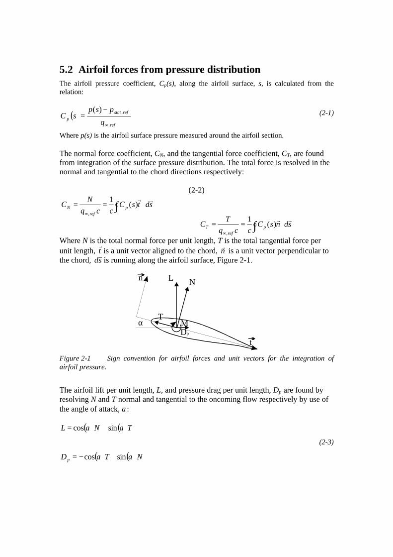
5.2 Airfoil forces from pressure distributionThe airfoil pressure coefficient, Cp(s), along the airfoil surface, s, is calculated from therelation:

(2-1)

Where p(s) is the airfoil surface pressure measured around the airfoil section.

The normal force coefficient, CN, and the tangential force coefficient, CT, are foundfrom integration of the surface pressure distribution. The total force is resolved in thenormal and tangential to the chord directions respectively:

(2-2)

Where N is the total normal force per unit length, T is the total tangential force perunit length,

rt is a unit vector aligned to the chord,

rn is a unit vector perpendicular to

the chord, dsr

is running along the airfoil surface, Figure 2-1.

NL

Dp

T

n

t

Mα

Figure 2-1 Sign convention for airfoil forces and unit vectors for the integration ofairfoil pressure.

The airfoil lift per unit length, L, and pressure drag per unit length, Dp are found byresolving N and T normal and tangential to the oncoming flow respectively by use ofthe angle of attack, α:

( ) ( )TNL αα sincos +=

(2-3)

( ) ( )NTDp αα sincos +−=

( )ref

refstat

p q

pspsC

,

,)(

∞

−=

∫ ⋅==∞

sdtsCccq

NC p

refN

rr)(

1

,

∫ ⋅==∞

sdnsCccq

TC p

refT

rr)(

1

,

The lift coefficient, CL, and pressure drag coefficient, CDp, are calculated:

cq

LC

refL

,∞

=

(2-4)

cq

DC

ref

pDp

,∞

=

The airfoil moment coefficient, CM, is found from integration of the contributionsfrom normal and tangential pressure components:

(2-5)

Where rr is a vector from the point of moment to the vector along the airfoil surface.

5.3 Airfoil drag from wake rakeThe airfoil total drag is the sum of contributions from skin friction and pressure drag. Sinceonly pressure drag can be calculated from the airfoil pressure distribution, the total drag iscalculated from a momentum balance between the momentum in the flow ahead of the airfoilsection with the momentum in the flow behind the airfoil section. It is then assumed that theflow is 2d.

The total wake drag coefficient, CDw, is calculated from [7]:

(2-6)

Where Ptot(y) is wake rake total pressure, pstat(y) is wake rake static pressure.

∫

−−⋅−=∞∞

dyq

ypyp

q

ypyp

cC

ref

stattot

ref

stattotDw

,,

)()(1

)()(2

( )( ) ( )( )[ ]∫∫ ⋅⋅+⋅⋅==∞

sdnsCnrsdtsCtrccq

MC PP

refM

rrrrrrrr)()(

122

,

6 Results

This chapter reports results from measurements on the NACA 63-215 airfoil. Thedifferent measurement runs are described in more detail in Appendix A1. All shownresults have been corrected for wind tunnel effects (Chapter 3) and are referenced tothe wind tunnel Pitot 1 reference established in Chapter 4.

First, detailed pressure distributions are presented. Next polar curves are shown forCL, CD and CM. Measurements are shown for leading edge roughness flow. Dynamicmeasurements are shown for the airfoil in pitching motion. Finally measurements athigh angles of attack are investigated for multiple CL levels at constant angle ofattack, the so-called ‘double stall’ phenomenon.

Five different types of measurements are used:

1. Measurements at different angles of attack with 20 s time series at each angle.Angle of attack range from -6o to 30o with discrete steps of 2o. Sample frequency 5Hz. See Appendix A1.1, measurement type, ‘STEP’.

2. Measurements at different angles of attack with continuous change of angle ofattack around 0.1 - 0.5 o/s. Angle of attack range from -6o to 30o. Sample frequency50 Hz. See Appendix A1.1, measurement type ‘CONT’.

3. Measurements at different angles of attack with time series length 180s at eachangle. Angles of attack in light and deep stall. Sample frequency 100 Hz. SeeAppendix A1.1, measurement type ‘STAT’.

4. Dynamic measurements with the airfoil section in pitching motion around differentmean angles of attack with amplitudes between 2° and 3o and different reducedfrequencies. Time series length 30s to 40s. Sample frequency 100 Hz. SeeAppendix A1.1, measurement type ‘PITCH’.

5. As measurement 2, ‘CONT’, with the use of sand paper at the leading edge tosimulate surface roughness.

The measurements were compared to measurements from FFA carried out on exactlythe same airfoil section model at Re = 1.7×106 in a closed wall wind tunnel [4] andNACA measurements at Re = 3.0×106 from [1].

The measurements were also compared to calculations. The XFOIL code based on apanel method with a viscous boundary layer formulation was used with free transitionmodeling and in cases with leading edge roughness with transition fixed to the leadingedge [16]. The EllipSys2D Navier-Stokes code was used for turbulent flowcalculations with the k-ω turbulence model without transition prediction [12].

6.1 Pressure distributionsF i g u r e 6 . 1 shows the measured CP curves for different angles ofattack. Each CP curve was based on average values for a 20s time series. When the angle ofattack was increased, the suction peak was gradually build up until angles of attack around

16o. At higher angles of attack, the airfoil stalled and separation removed the suction peak andthe suction side pressure became nearly uniform.

Risø-R-981(EN)42

-2

-1.5

-1

-0.5

0

0.5

10 0.2 0.4 0.6 0.8 1

CP

x/c

α = -3.7o

α = -2.1o

α = -0.5o

α = 1.1o

α = 2.8o

α = 4.5o

-7.0

-6.0

-5.0

-4.0

-3.0

-2.0

-1.0

0.0

1.00 0.2 0.4 0.6 0.8 1

CP

x/c

α = 6.1o

α = 7.8o

α = 9.5o

α = 11.4o

α = 13.2o

α = 15.3o

-2

-1.5

-1

-0.5

0

0.5

10 0.2 0.4 0.6 0.8 1

CP

x/c

α = 18.1o

α = 20.3o

α = 22.3o

α = 24.3o

α = 26.2o

α = 28.3o

Figure 6-1 Measured CP curves at different angles of attack(NA63215STEP290296V1).

Risø-R-981(EN) 43

Figure 6-2 shows a CP curve at α = 7.8° with minimum and maximum valuesfor a 20s time series. The standard deviation was small on the pressure side andslightly increased at the suction peak.

-4

-3

-2

-1

0

10 0.2 0.4 0.6 0.8 1

CP

x/c

MeanMinMax

Figure 6-2 Measured CP curve with minimum and maximum values, NACA 63-215, Re = 1.3×106, α = 7.8°, (NA63215STEP290296V1).

Figure 6-3 shows the measured CP curve at α = 7.8o compared to an EllipSys2Dturbulent flow calculation and an XFOIL free transition calculation. Theagreement with both computations was good. The suction peak was wellcaptured in the measurement and the stagnation pressure was located at thesame position. Near the trailing edge there was a small discrepancy with lowerpressures for the measurement compared to the calculations. This was causedby the deviation in the tested model compared to the theoretical coordinates,Section 2.3. This deviation will however not influence the calculation ofaerodynamic loads.

-4

-3

-2

-1

0

10 0.2 0.4 0.6 0.8 1

CP

x/c

RISOEllipSys2D

XFOIL

Figure 6-3 Measured CP curve compared to EllipSys2D (turbulent flow) andXFOIL free transition calculations, NACA 63-215, Re = 1.3×106, α = 7.8o,(NA63215STEP290296V1).

Risø-R-981(EN)44

The measured CP curve α = 6.1o is compared to a FFA measurement [4] and anXFOIL free transition calculation in Figure 6-4. The suction peak and thestagnation point were in good agreement. The shape of the CP curve was ingeneral captured quite well and the deviations were minor. At the trailing edgehowever, the XFOIL calculation resulted in higher pressures compared to themeasurements as in Figure 6-3.

-2.5

-2

-1.5

-1

-0.5

0

0.5

10 0.2 0.4 0.6 0.8 1

CP

x/c

RISO, Re = 1.3x106, α = 6.1o

FFA, Re = 1.7x106, α = 5.7o

XFOIL, Re = 1.3x106, α = 5.9o

Figure 6-4 Measured CP curve, Re = 1.3×106, at α = 6.1o compared to FFAmeasurement, Re = 1.7×106, at α = 5.7o [4] and XFOIL free transitioncalculation, Re = 1.3×106, at α = 5.9o (NA63215STEP290296V1).

A corresponding comparison at α = 11.4o shows the same tendencies, Figure6-5, although the suction peak is overestimated by XFOIL. The FFA and theRisø measurements were in good agreement, whereas the XFOIL calculationshowed higher pressures at the trailing edge.

-7

-6

-5

-4

-3

-2

-1

0

10 0.2 0.4 0.6 0.8 1

CP

x/c

RISO, Re = 1.3x106, α = 11.4o

FFA, Re = 1.7x106, α = 11.1o

XFOIL, Re = 1.3x106, α = 11.2o

Figure 6-5 Measured CP curve, Re = 1.3×106, at α = 11.4o compared to FFAmeasurement, Re = 1.7×106, at α = 11.1o [4] and XFOIL free transitioncalculation, Re = 1.3×106, at α = 11.2o (NA63215STEP290296V1).

Risø-R-981(EN) 45

Figure 6-6 shows the measured CP curve at α = 15.3o compared to an FFAmeasurement and an XFOIL free transition calculation. The stagnation pointswere located similar and the pressure sides were in good agreement. On thesuction side, separation has started from the trailing edge. On the trailing edgepart, the agreement between the FFA and Risø measurements was good. Thedegree of separation was higher for the Risø measurement, compared with FFA.This could be caused by the higher turbulence intensity in the Risømeasurement that would advance transition and separation.

Since the blocking effects are higher in the FFA closed wall tunnel and takinginto consideration the difference in Reynolds number, it is possible that theacceleration of the flow reduced relatively the occurrence of separation in theFFA measurement compared to the Risø measurement.

-7

-6

-5

-4

-3

-2

-1

0

10 0.2 0.4 0.6 0.8 1

CP

x/c

RISO, Re = 1.3x106, α = 15.3o

FFA, Re = 1.7x106, α = 15.0o

XFOIL, Re = 1.3x106, α = 15.0o

Figure 6-6 Measured CP curve, Re = 1.3×106, at α = 15.3o compared to FFAmeasurement, Re = 1.7×106, at α = 15.0o [4] and XFOIL free transitioncalculation, Re = 1.3×106, at α = 15.0o (NA63215STEP290296V1).

Figure 6-7 shows measured CP at α = 18.1o compared to FFA measurements.The agreement on the pressure side was fair, whereas the suction sides differedtowards the trailing edge. The highly unsteady flow at this angle was clearlydifferent in the two wind tunnels and the measured results were not comparablefor high angles of attack.

Risø-R-981(EN)46

-2

-1.5

-1

-0.5

0

0.5

10 0.2 0.4 0.6 0.8 1

CP

x/c

RISO, Re = 1.3x106, α = 18.1o

FFA, Re = 1.7x106, α = 17.9o

Figure 6-7 Measured CP curve, Re = 1.3×106, at α = 18.1o compared to FFAmeasurements, Re = 1.7×106, at α = 17.9o [4] (NA63215STEP290296V1).

6.2 Polar resultsThis section presents the aerodynamic loads on the airfoil section that arecalculated from the airfoil pressure and wake rake measurements. Wind tunnelboundary corrections were applied to all reported results.

Lift coefficient

The measured CL curve with minimum and maximum values is shown in Figure6-8. Each measurement points represents a 20s time series, sampled with 5 Hz.The standard deviation was in general very low except for the post stall region,where the flow was highly unsteady and 3d.

-0.5

0

0.5

1

1.5

-5 0 5 10 15 20 25

CL

α

MeanMinMax

Figure 6-8 Measured CL curve with minimum and maximum values for a 20 stime series (NA63215STEP290296V1).

Risø-R-981(EN) 47

The measured CL curve is shown in Figure 6-9 compared to an XFOIL freetransition calculation and an EllipSys2D turbulent flow calculation, both at Re= 1.3×106.

There was in general good agreement. At low angles of attack, the three curveswere nearly identical. The slope of the measured curve was slightly lowercompared to the calculated curves. This was probably because the correctionsfor streamline curvature and down-wash were too small. The influence ofdown-wash through the clearance between the airfoil section and the endplatescould be underestimated or the streamline curvature might not be perfectlycomparable to the cascade flow that forms the basis for the applied correction.However, the agreement was satisfactory.

At higher angles of attack, the measured CL curve did not agree well with thecalculation. CLmax was measured too low and CL was measured too low in thepost stall region. This is however often seen when measurements are comparedto calculations. Especially XFOIL calculations tend to show too high CLmax

together with too steep CL curve slope [16].

Figure 6-10 shows the measured CL curve from Figure 6-9 compared tomeasurements from FFA [4] carried out on exactly the same airfoil section atRe = 1.7×106 in a closed wall wind tunnel and NACA measurements from [1] atRe = 3.0×106. The CL curve slopes at low angles of attack were in goodagreement. The NACA measurement was slightly offset to a different angle ofzero lift. The slope of the FFA measurement was steeper than the Risømeasurement. The agreement between Risø and FFA measurements was gooduntil 15° and at CLmax. However, the post stall area was very different for the twomeasurements probably because of different 3d behavior of the wind tunneltypes that were used.

-0.5

0

0.5

1

1.5

-5 0 5 10 15 20 25

CL

α

RISOXFOIL

EllipSys2D

Figure 6-9 Measured CL curve compared to XFOIL free transition calculationand EllipSys2D turbulent flow calculation at Re = 1.3×106

(NA63215STEP290296V1).

Risø-R-981(EN)48

-0.5

0

0.5

1

1.5

-5 0 5 10 15 20 25

CL

α

RISO, Re = 1.3x106

FFA, Re = 1.7x106

NACA, Re = 3.0x106

Figure 6-10 Measured CL curve at Re = 1.3×106, compared to FFAmeasurements, Re = 1.7×106 [4] and NACA measurements, Re = 3.0×106 [1](NA63215STEP290296V1).

The established wind tunnel reference and the applied wind tunnel boundarycorrections turned out to give good results. Even though the FFA measurementsappears to be even closer to the calculations, the agreement between Risø andFFA measurements was good, having in mind the uncertainties introduced bythe open jet flow.

Drag coefficient

The measured CD curves with mean, minimum and maximum values are shownin Figure 6-11, based on 20s time series, sampled with 5 Hz, at each angle ofattack. At angles of attack below app. 13o, the drag was calculated from thewake rake. At higher angles of attack, when the drag from the pressuredistribution increased because of separation, the drag was taken simply as thedrag from the pressure distribution.

0

0.02

0.04

0.06

0.08

0.1

-5 0 5 10 15 20

CD

α

MeanMinMax

Figure 6-11 Measured CD curve, Re = 1.3×106, with minimum and maximumvalues for 20s time series (NA63215STEP290296V1).

Risø-R-981(EN) 49

Compared to the CL, CD is more complex to determine with high accuracybecause of the calibration of the wake rake and the disturbances from theendplates downstream of the airfoil section. Compared to the value of CD, thestandard deviation appears to be quite high.

The measured CD curve is compared with XFOIL free transition calculationsand EllipSys2D turbulent flow calculations in Figure 6-12. The shape of the CD

curve was captured well in the measurement compared to the XFOILcalculation. Around 5° there is a small jump in drag, which is also predicted byXFOIL at 6°. Normally, XFOIL predicts drag very well at low angles of attack[16]. However XFOIL maintains attached flow until a higher angle of attackand hence underestimates drag at higher angles of attack. This explains thediscrepancy between measurements and XFOIL calculations at higher angles ofattack. The higher skin friction from a fully turbulent boundary layer flowcaused the rather high drag at low angles of attack predicted by EllipSys2Dcompared to measurements. EllipSys2D predicts the increase in drag afterseparation well compared to XFOIL.

0

0.02

0.04

0.06

0.08

0.1

-5 0 5 10 15 20

CD

α

RISOXFOIL

EllipSys2D

Figure 6-12 Measured CD curve compared to XFOIL free transition calculationand EllipSys2D turbulent flow calculation at Re = 1.3×106,(NA63215STEP290296V1).

Figure 6-13 shows the measured CD curve from Figure 6-12 compared to theFFA measurement [4] and the NACA measurement [1]. While the tendency ofCD was well captured, the measured CD was slightly higher in absolute valuescompared to the NACA and FFA measurements. This offset was probably dueto the higher turbulence in the tunnel, see chapter 4.

Risø-R-981(EN)50

0

0.02

0.04

0.06

0.08

0.1

-5 0 5 10 15 20

CD

α

RISO, Re = 1.3x106

FFA, Re = 1.7x106

NACA, Re = 3.0x106

Figure 6-13 Measured CD curve, Re = 1.3×106, compared to FFAmeasurements, Re = 1.3×106, [4] and NACA measurements, Re = 1.3×106, [1](NA63215STEP290296V1).

Moment coefficient

The measured CM curves with mean, minimum and maximum values are shownin Figure 6-14. Each measurement point was based on a 20 s time series,sampled with 5 Hz. The standard deviation was very low at low angles of attackwhereas it increased significantly in the post stall area.

The measured CM curve is shown in Figure 6-15 compared to the FFAmeasurement [4], NACA measurement [1] and an XFOIL free transitioncalculation. The Risø measurements were in good agreement with the NACAmeasurements and at low angles of attack the agreement was in general good.The FFA measurements compared well to the XFOIL calculations. The

-0.2

-0.15

-0.1

-0.05

0

-5 0 5 10 15 20 25

CM

α

MeanMinMax

Figure 6-14 Measured CM curve, Re = 1.3×106, with minimum and maximumvalues for 20s time series (NA63215STEP290296V1).

Risø-R-981(EN) 51

deviations between the Risø measurement and the FFA measurement were duedifferent influence from the wind tunnel.

-0.2

-0.15

-0.1

-0.05

0

-5 0 5 10 15 20 25

CM

α

RISO, Re = 1.3x106

FFA, Re = 1.7x106

NACA, Re = 3.0x106

XFOIL, Re = 1.3x106

Figure 6-15 Measured CM curve, Re = 1.3×106, compared to FFAmeasurements, Re = 1.7×106, [4], NACA measurements, Re = 3.0×106, [1] andXFOIL free transition calculation, Re = 1.3×106, (NA63215STEP290296V1).

6.3 Leading edge roughnessIn natural conditions, bugs and dirt often soil wind turbine blades. Thesensitivity of the wind turbine power production to this is important. Byapplying leading edge roughness (LER) to the airfoil section leading edge, soildepositing can be simulated to investigate the airfoil performance under thiscondition. The applied leading edge roughness was described in Section 2.6.

Pressure distributions

Figure 6-16 shows measured CP at α = 11.0o for leading edge roughnesscompared to smooth flow. Whereas the pressure side was nearly unaffected byLER, the suction side pressure distribution was different compared with thecorresponding smooth flow condition. The suction side pressure at the leadingedge part was higher resulting in lower CL. The presence of LER influenced thevelocity distribution close to the airfoil surface where velocity was reduced andthe degree of separation was higher in the rough case. Following the velocityreduction, the suction peak was also reduced.

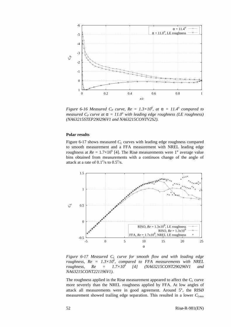
Risø-R-981(EN)52

-6

-5

-4

-3

-2

-1

0

10 0.2 0.4 0.6 0.8 1

CP

x/c

α = 11.4o

α = 11.0o, LE roughness

Figure 6-16 Measured CP curve, Re = 1.3×106, at α = 11.4o compared tomeasured CP curve at α = 11.0o with leading edge roughness (LE roughness)(NA63215STEP290296V1 and NA63215CONTV2S2).

Polar results

Figure 6-17 shows measured CL curves with leading edge roughness comparedto smooth measurement and a FFA measurement with NREL leading edgeroughness at Re = 1.7×106 [4]. The Risø measurements were 1° average valuebins obtained from measurements with a continuos change of the angle ofattack at a rate of 0.1o/s to 0.5o/s.

-0.5

0

0.5

1

1.5

-5 0 5 10 15 20 25

CL

α

RISO, Re = 1.3x106, LE roughnessRISO, Re = 1.3x106

FFA, Re = 1.7x106, NREL LE roughness

Figure 6-17 Measured CL curve for smooth flow and with leading edgeroughness, Re = 1.3×106, compared to FFA measurements with NRELroughness, Re = 1.7×106 [4] (NA63215CONT290296V1 andNA63215CONT221196V1).

The roughness applied in the Risø measurement appeared to affect the CL curvemore severely than the NREL roughness applied by FFA. At low angles ofattack all measurements were in good agreement. Around 5°, the RISØmeasurement showed trailing edge separation. This resulted in a lower CLmax

Risø-R-981(EN) 53

compared to the other measurements. In the post stall region there were largedeviations.

The CD curve with leading edge roughness corresponding to CL in Figure 6-17is shown in Figure 6-18. At low angles of attack below 0° there was goodagreement between FFA and Risø LER measurements. CD is higher for LERcompared to smooth flow as expected. Before separation, CD tended to increasefor the Risø measurement compared to the FFA measurement, due to the moresevere roughness. Separation occurred earlier for the Risø LER measurementcompared the FFA measurement.

0

0.02

0.04

0.06

0.08

0.1

-5 0 5 10 15 20

CD

α

RISO, Re = 1.3x106, LE roughnessRISO, Re = 1.3x106

FFA, Re = 1.7x106, NREL LE roughness

Figure 6-18 Measured CD curve for smooth flow and with leading edgeroughness, Re = 1.3×106, compared to FFA measurements with NRELroughness, Re = 1.7×106 [4] (NA63215CONT290296V1 andNA63215CONT221196V1).

Figure 6-19 shows the measured CM curve for smooth and rough conditionscorresponding to Figure 6-17. The leading edge roughness does not affect CM atlow angles of attack, whereas the drop in CM at separation was shifted to alower angle of attack due to the earlier separation of the flow. The differencebetween Risø measurements and FFA measurements corresponds to that ofsmooth flow.

Risø-R-981(EN)54

-0.2

-0.15

-0.1

-0.05

0

-5 0 5 10 15 20 25

CM

α

RISO, Re = 1.3x106, LE roughnessRISO, Re = 1.3x106

FFA, Re = 1.7x106, NREL LE roughness

Figure 6-19 Measured CM curve for smooth flow and with leading edgeroughness, Re = 1.3×106, compared to FFA measurements with NRELroughness, Re = 1.7×106 [4] (NA63215CONT290296V1 andNA63215CONT221196V1).

6.4 Dynamic stallThe aerodynamic loads on the airfoil section were measured while the airfoilwas in pitching motion. This comprises dynamic stall measurements, which arevery important to the dynamics at high wind speeds for stall regulated windturbines.

When the angle of attack is changed, the aerodynamic loading on the airfoil isaltered and vortices are shed from the airfoil leading edge. Because of theinteraction of the vortices with the flow and the travel time of these vorticesalong the airfoil surface and in the airfoil wake, there will be a time lagbetween changes in the angle of attack and changes in the aerodynamic loading.This time lag causes a hysteresis effect on the relation between the angle ofattack and the aerodynamic loads and hysteresis loops appear for theaerodynamic forces. The size of the hysteresis loops varies with the type ofairfoil flow, the amplitude of the pitching motion and the reduced frequency ofthe flow. When the airfoil suction side is partially or entirely separated, theloops become open compared to the loops at angles of attack with attachedflow.

The pitching motion is related to the reduced frequency, k, which is defined as:

(6-1)

Where ω = 2π f is the angular velocity of the pitching motion, f is thefrequency, c is the airfoil chord and V∞ is the free stream velocity.

Figure 6-20 shows a sample of a time series of the angle of attack with theairfoil in pitching motion at k = 0.044 corresponding to a frequency of 1.17 Hz.The amplitude was 2.5° with a mean angle of attack of 7.6o. Compared to a

∞

=V

ck

2

ω

Risø-R-981(EN) 55

pure harmonic motion there appeared to be some disturbances that come fromspikes and electrical noise but also from vibrations of the test stand. Theelectric motor that runs the pitching mechanism had too low power resulting indifficulties in maintaining a smooth motion.

4

5

6

7

8

9

10

11

10 11 12 13 14 15

α

t

k = 0.044

Figure 6-20 Raw data angle of attack time series (NA63215PITCH220296V1).

To improve the quality of the time series, we filtered the data by applyingmoving averages with a frame of 0.1s. The result is shown in Figure 6-21. Thisremoved the spikes and made the curve smooth but it also reduced minimumand maximum values slightly.

4

5

6

7

8

9

10

11

10 11 12 13 14 15

α

t

k = 0.044

Figure 6-21 Angle of attack time series with 0.1s moving average(NA63215PITCH220296V1).

The PSD spectrums for both time series are shown in Figure 6-22. It can beseen that the dominating frequency was the pitching motion on 1.17 Hz,whereas no resonance appeared at higher frequencies. The moving average didnot influence frequencies below 4 Hz, but did reduce noise at higherfrequencies with more than one decade.

Risø-R-981(EN)56

1e-006

1e-005

0.0001

0.001

0.01

0.1

1

10

100

0 2 4 6 8 10

PSD

f

Figure 6-22 PSD of the angle of attack time series from Figure 6-20 andFigure 6-21 (NA63215PITCH220296V1).

Dynamic hysteresis loops

Figure 6-23 shows CL versus angle of attack for the moving averaged timeseries shown in Figure 6-21. The tendency for the hysteresis loop was clearlyseen, but the different loops were not identical because of small differences inthe flow and measurement uncertainties.

0.6

0.7

0.8

0.9

1

1.1

1.2

1.3

1.4

4 5 6 7 8 9 10 11

CL

α

k = 0.044

Figure 6-23 CL hysteresis loops corresponding to the time series in Figure 6-21(NA63215PITCH220296V1).

To obtain an averaged loop, the angles of attack were divided into 30 bins of aphase angle, which runs from 0 to 2π at each loop. This resulted in the averageloop that can be seen in Figure 6-24. Both raw data and moving averaged datawere sorted in bins and the comparison shows that the moving average does notchange the loop except for minor differences in minimum and maximum angleof attack.

Risø-R-981(EN) 57

The direction of the hysteresis loops is important for the aerodynamic damping.The direction can be found by comparison of the change in the angle of attackwith the phase angle. The direction in Figure 6-24 was counterclockwise.

0.6

0.7

0.8

0.9

1

1.1

1.2

1.3

1.4

4 5 6 7 8 9 10 11

CL

α

Raw data0.1 s moving average

Figure 6-24 CL hysteresis loop for raw data and moving averaged date sortedin 30 bins of a phase angle running from o to 2π at each pitching period(NA63215PITCH220296V1).

Reduced frequency k = 0.044

A series of seven different measurements was taken at k = 0.044, withamplitudes between 2.5° and 3.0° for different mean angles of attack coveringboth attached and separated flow.

The CL, CD and CM hysteresis loops are shown in Figure 6-25, Figure 6-26 andFigure 6-27 respectively. CD measurements were based on pressure drag only.Arrows indicate the directions of the loops. The steady curves are shown forcomparison. For CD and CM there are small discrepancies between the level ofthe hysteresis loops and the steady mean curve caused by uncertainties fromcalibration of the measurement system.

The amplitude of the hysteresis loops varied between 2.5° and 3.0°. The rawdata angle of attack amplitude was 3.0° but the wind tunnel boundarycorrections, where α depend on CL, caused a difference in amplitude.

Risø-R-981(EN)58

-0.2

-0.1

0

0.1

0.2

0.3

0.4

0.5

-3 -2 -1 0 1 2C

Lα

k = 0.044, αm = -0.6o, A = 2.6o

0.3

0.4

0.5

0.6

0.7

0.8

0.9

1

1 2 3 4 5 6

CL

α

k = 0.044, αm = 3.4o, A = 2.5o

0.7

0.8

0.9

1

1.1

1.2

1.3

1.4

5 6 7 8 9 10

CL

α

k = 0.044, αm = 7.6o, A = 2.5o

1

1.1

1.2

1.3

1.4

1.5

1.6

1.7

9 10 11 12 13 14 15

CL

α

k = 0.044, αm = 11.9o, A = 2.7o

0.8

0.9

1

1.1

1.2

1.3

1.4

1.5

15 16 17 18 19 20

CL

α

k = 0.044, αm = 17.4o, A = 3.0o

0.5

0.6

0.7

0.8

0.9

1

1.1

1.2

19 20 21 22 23 24 25

CL

α

k = 0.044, αm = 22.1o, A = 2.9o

0.5

0.6

0.7

0.8

0.9

1

1.1

1.2

25 26 27 28 29 30

CL

α

k = 0.044, αm = 27.4o, A = 2.8o

Figure 6-25 Measured CL hysteresis loops for smooth flow at k = 0.044, Abetween 2.5° and 3.0°, Re = 1.3×106 (NA63215PITCH220296V1).

Risø-R-981(EN) 59

-0.1

-0.05

0

0.05

0.1

0.15

0.2

-3 -2 -1 0 1 2

CD

α

k = 0.044, αm = -0.6o, A = 2.6o

-0.1

-0.05

0

0.05

0.1

0.15

0.2

1 2 3 4 5 6

CD

α

k = 0.044, αm = 3.4o, A = 2.5o

-0.1

-0.05

0

0.05

0.1

0.15

0.2

5 6 7 8 9 10

CD

α

k = 0.044, αm = 7.6o, A = 2.5o

-0.1

-0.05

0

0.05

0.1

0.15

0.2

9 10 11 12 13 14 15

CD

α

k = 0.044, αm = 11.9o, A = 2.7o

0.1

0.15

0.2

0.25

0.3

0.35

0.4

15 16 17 18 19 20

CD

α

k = 0.044, αm = 17.4o, A = 3.0o

0.25

0.3

0.35

0.4

0.45

0.5

0.55

19 20 21 22 23 24 25

CD

α

k = 0.044, αm = 22.1o, A = 2.9o

0.35

0.4

0.45

0.5

0.55

0.6

0.65

25 26 27 28 29 30

CD

α

k = 0.044, αm = 27.4o, A = 2.8o

Figure 6-26 Measured CD hysteresis loops for smooth flow at k = 0.044, Abetween 2.5° and 3.0°, Re = 1.3×106 (NA63215PITCH220296V1).

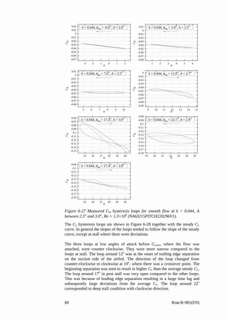
Risø-R-981(EN)60

-0.07-0.06-0.05-0.04-0.03-0.02-0.01

00.010.02

-3 -2 -1 0 1 2C

Mα

k = 0.044, αm = -0.6o, A = 2.6o

-0.08-0.07-0.06-0.05-0.04-0.03-0.02-0.01

00.01

1 2 3 4 5 6

CM

α

k = 0.044, αm = 3.4o, A = 2.5o

-0.08-0.07-0.06-0.05-0.04-0.03-0.02-0.01

00.01

5 6 7 8 9 10

CM

α

k = 0.044, αm = 7.6o, A = 2.5o

-0.09-0.08-0.07-0.06-0.05-0.04-0.03-0.02-0.01

0

9 10 11 12 13 14 15

CM

α

k = 0.044, αm = 11.9o, A = 2.7o

-0.15-0.14-0.13-0.12-0.11-0.1

-0.09-0.08-0.07-0.06

15 16 17 18 19 20

CM

α

k = 0.044, αm = 17.4o, A = 3.0o

-0.18-0.17-0.16-0.15-0.14-0.13-0.12-0.11-0.1

-0.09-0.08

19 20 21 22 23 24 25

CM

α

k = 0.044, αm = 22.1o, A = 2.9o

-0.18-0.17-0.16-0.15-0.14-0.13-0.12-0.11-0.1

-0.09

25 26 27 28 29 30

CM

α

k = 0.044, αm = 27.4o, A = 2.8o

Figure 6-27 Measured CM hysteresis loops for smooth flow at k = 0.044, Abetween 2.5° and 3.0°, Re = 1.3×106 (NA63215PITCH220296V1).

The CL hysteresis loops are shown in Figure 6-28 together with the steady CL

curve. In general the slopes of the loops tended to follow the slope of the steadycurve, except at stall where there were deviations.

The three loops at low angles of attack before CLmax, where the flow wasattached, were counter clockwise. They were more narrow compared to theloops at stall. The loop around 12o was at the onset of trailing edge separationon the suction side of the airfoil. The direction of the loop changed fromcounter-clockwise to clockwise at 10o, where there was a crossover point. Thebeginning separation was seen to result in higher CL than the average steady CL.The loop around 17o in post stall was very open compared to the other loops.This was because of leading edge separation resulting in a large time lag andsubsequently large deviations from the average CL. The loop around 22o

corresponded to deep stall condition with clockwise direction.

Risø-R-981(EN) 61

-0.5

0

0.5

1

1.5

-5 0 5 10 15 20 25

CL

α

k = 0.044

Figure 6-28 Measured CL hysteresis loops at k=0.044(NA63215PITCH220296V1).

Figure 6-29 shows CD hysteresis loops based on pressure drag compared to thesteady CD curve from pressure drag. Since the wake rake measured the flowdownstream of the airfoil there would be a time delay compared to the pressuremeasurements on the airfoil. Because of the unsteady loading, this delay madeit impossible to use the wake rake.

-0.05

0

0.05

0.1

0.15

0.2

0.25

0.3

0.35

0.4

0.45

-5 0 5 10 15 20 25

CD

α

k = 0.044

Figure 6-29 Measured CD hysteresis loops at k=0.044(NA63215PITCH220296V1).

There was a small deviation between mean CD for the loops and the CD meancurve caused by calibration uncertainties of the raw measurements. Thetendencies from CL regarding narrow and closed loops were also seen on CD.However there were differences in the directions of the loops. The main part ofthe first loop was counterclockwise with a crossover point around 0°. Above 0°,the direction changed to clockwise. The next two loops were clockwise. Theloop around 12o was clockwise towards low angles of attack but counter-clockwise toward 15o. The two loops in stall were both counter-clockwise.

Risø-R-981(EN)62

The CM hysteresis loops are shown in Figure 6-30. The loops were in generalmore closed and their slopes tended to follow the mean line curve well. Atangles of attack below 12o the directions were counterclockwise. The directionsthen changed to clockwise until 18o, after which it again changes to counter-clockwise.

-0.2

-0.15

-0.1

-0.05

0

-5 0 5 10 15 20 25

CM

α

k = 0.044

Figure 6-30 Measured CM hysteresis loops at A=6o, k=0.044(NA63215PITCH220296V1).

Reduced frequency k = 0.022

A series of seven different measurements was taken at k = 0.022, withamplitudes between 2.5° and 3.3° for different mean angles of attack coveringboth attached and separated flow.

The individual CL, CD and CM hysteresis loops are shown in Figure 6-31, Figure6-32 and Figure 6-33. CD measurements were based on pressure drag only. Themean value curves were shown for comparison.Figure 6-34, Figure 6-35 and Figure 6-36 shows hysteresis loops for CL, CD andCM respectively at k = 0.022.

The curves were in agreement with the curves for k = 0.044, however the loopswere more narrow and the slopes of the loops at stall were reduced since thetime lag between changes of the angle of attack and the airfoil loading wassmaller.

Risø-R-981(EN) 63

-0.2

-0.1

0

0.1

0.2

0.3

0.4

0.5

-3 -2 -1 0 1 2

CL

α

k = 0.022, αm = -0.6o, A = 2.6o

0.3

0.4

0.5

0.6

0.7

0.8

0.9

1

1 2 3 4 5 6

CL

α

k = 0.022, αm = 3.3o, A = 2.5o

0.7

0.8

0.9

1

1.1

1.2

1.3

1.4

4 5 6 7 8 9 10

CL

α

k = 0.022, αm = 7.2o, A = 2.5o

1

1.1

1.2

1.3

1.4

1.5

1.6

1.7

9 10 11 12 13 14

CL

α

k = 0.022, αm = 11.5o, A = 2.7o

0.9

1

1.1

1.2

1.3

1.4

1.5

1.6

14 15 16 17 18 19

CL

α

k = 0.022, αm = 16.7o, A = 3.3o

0.5

0.6

0.7

0.8

0.9

1

1.1

1.2

20 21 22 23 24 25

CL

α

k = 0.022, αm = 22.5o, A = 3.0o

0.5

0.6

0.7

0.8

0.9

1

1.1

1.2

25 26 27 28 29 30

CL

α

k = 0.022, αm = 27.4o, A = 2.9o

Figure 6-31 Measured CL hysteresis loops for smooth flow at k = 0.022, Abetween 2.5° and 3.3°, Re = 1.3×106 (NA63215PITCH220296V2).

Risø-R-981(EN)64

-0.1

-0.05

0

0.05

0.1

0.15

0.2

-3 -2 -1 0 1 2C

Dα

k = 0.022, αm = -0.6o, A = 2.6o

-0.1

-0.05

0

0.05

0.1

0.15

0.2

1 2 3 4 5 6

CD

α

k = 0.022, αm = 3.3o, A = 2.5o

-0.1

-0.05

0

0.05

0.1

0.15

0.2

4 5 6 7 8 9 10

CD

α

k = 0.022, αm = 7.2o, A = 2.5o

-0.1

-0.05

0

0.05

0.1

0.15

0.2

9 10 11 12 13 14

CD

α

k = 0.022, αm = 11.5o, A = 2.7o

0.05

0.1

0.15

0.2

0.25

0.3

0.35

14 15 16 17 18 19

CD

α

k = 0.022, αm = 16.7o, A = 3.3o

0.25

0.3

0.35

0.4

0.45

0.5

0.55

20 21 22 23 24 25

CD

α

k = 0.022, αm = 22.5o, A = 3.0o

0.35

0.4

0.45

0.5

0.55

0.6

0.65

25 26 27 28 29 30

CD

α

k = 0.022, αm = 27.4o, A = 2.9o

Figure 6-32 Measured CD hysteresis loops for smooth flow at k = 0.022, Abetween 2.5° and 3.3°, Re = 1.3×106 (NA63215PITCH220296V2).

Risø-R-981(EN) 65

-0.07-0.06-0.05-0.04-0.03-0.02-0.01

00.010.02

-3 -2 -1 0 1 2

CM

α

k = 0.022, αm = -0.6o, A = 2.6o

-0.08-0.07-0.06-0.05-0.04-0.03-0.02-0.01

00.01

1 2 3 4 5 6

CM

α

k = 0.022, αm = 3.3o, A = 2.5o

-0.08-0.07-0.06-0.05-0.04-0.03-0.02-0.01

00.01

4 5 6 7 8 9 10

CM

α

k = 0.022, αm = 7.2o, A = 2.5o

-0.09-0.08-0.07-0.06-0.05-0.04-0.03-0.02-0.01

0

9 10 11 12 13 14

CM

α

k = 0.022, αm = 11.5o, A = 2.7o

-0.14-0.13-0.12-0.11-0.1

-0.09-0.08-0.07-0.06-0.05

14 15 16 17 18 19

CM

α

k = 0.022, αm = 16.7o, A = 3.3o

-0.17-0.16-0.15-0.14-0.13-0.12-0.11-0.1

-0.09-0.08

20 21 22 23 24 25

CM

α

k = 0.022, αm = 22.5o, A = 3.0o

-0.18-0.17-0.16-0.15-0.14-0.13-0.12-0.11-0.1

-0.09

25 26 27 28 29 30

CM

α

k = 0.022, αm = 27.4o, A = 2.9o

Figure 6-33 Measured CM hysteresis loops for smooth flow at k = 0.022, Abetween 2.5° and 3.3°, Re = 1.3×106 (NA63215PITCH220296V2).

Risø-R-981(EN)66

-0.5

0

0.5

1

1.5

-5 0 5 10 15 20 25

CL

α

k = 0.022

Figure 6-34 Measured CL hysteresis loops at k=0.022(NA63215PITCH220296V2).

-0.05

0

0.05

0.1

0.15

0.2

0.25

0.3

0.35

0.4

0.45

-5 0 5 10 15 20 25

CD

α

k = 0.022

Figure 6-35 Measured CD hysteresis loops at k = 0.022(NA63215PITCH220296V2).

Risø-R-981(EN) 67

-0.2

-0.15

-0.1

-0.05

0

-5 0 5 10 15 20 25

CM

α

k = 0.022

Figure 6-36 Measured CM hysteresis loops at k = 0.022(NA63215PITCH220296V2).

6.5 Double stallThis section contains investigations of time series during stall at high angles ofattack. The aim is to determine the stability of the flow. In the references, [13]and [14] it is reported that the NACA 63-215 has different CL levels at stall foridentical inflow conditions. This is the so-called ‘double stall’ phenomenon[13]. The purpose with this section is to reveal the difference between the flowstates at these levels and eventually identify the trigger for the different levels.

Measurements were performed at different angles of attack in stall. Initially,there were no signs of ‘double stall’. Few measurements were taken where theclearance between the airfoil section and the endplates were sealed with tape,since this further improves the 2d behavior of the flow. One measurement thenshowed signs of ‘double stall’. Figure 6-37 shows the time series of CL for theNACA 63-215 airfoil at approximately α = 15.3o. This corresponds to anuncorrected α on 18.0o. The sample frequency was 100 Hz, so 18000 framescorrespond to 180 s. It can be seen, that initially the CL was around 0.9 - 1.0 atthe low lift level. At approximately 1250 frames, CL suddenly increased to thehigh lift level at 1.2 - 1.3. For a long period, CL remained at this high with levela few short stays on an intermediate level at 1.1 - 1.2. After around 12800frames CL suddenly changed to the intermediate lift level. In total 3 differentstall levels appeared with clear difference in CL.

Risø-R-981(EN)68

0.6

0.7

0.8

0.9

1

1.1

1.2

1.3

1.4

1.5

0 2000 4000 6000 8000 10000 12000 14000 16000 18000

CL

frame

α = 15.3o

Figure 6-37 Measured CL time series at α = 15.3o (18o uncorrected). 100frames correspond to 1 second (NA63215STAT221196V1).

The corresponding CD curve is shown in Figure 6-38. At the low lift level, CD

was around 0.2 - 0.25 with a high standard deviation. At the high lift level, CD

was reduced to 0.08 - 0.1 with much smaller standard deviation. Finally, CD

appeared to be at 0.1 at the intermediate lift level.

0.05

0.1

0.15

0.2

0.25

0.3

0.35

0 2000 4000 6000 8000 10000 12000 14000 16000 18000

CD

frame

α = 15.3o

Figure 6-38 Measured CD time series at α = 15.3o (18o uncorrected). 100frames correspond to 1 second (NA63215STAT221196V1).

Figure 6-39 shows CM for the same time series. At the low lift level, CM wasaround -0.12 - 0.14. At the high lift level, CM was increased to around -0.075.At the intermediate lift level, CM was around -0.08 but with increased standarddeviation compared to the high level.

Risø-R-981(EN) 69

-0.18

-0.16

-0.14

-0.12

-0.1

-0.08

-0.06

-0.04

0 2000 4000 6000 8000 10000 12000 14000 16000 18000

CM

frame

α = 15.3o

Figure 6-39 Measured CM time series at α = 15.3o (18o uncorrected). 100frames correspond to 1 second (NA63215STAT221196V1).

Figure 6-40 shows time averaged CP curves for the different CL levels. The lowlevel had only a small suction peak, after which the flow was separated at 15 -20% chord. The stagnation point was moved slightly toward the leading edgecompared to the higher lift levels. The pressure difference on the trailing edgepart of the airfoil was bigger compared to the other levels, however the lack ofsuction pressure resulted in reduced CL.

-7

-6

-5

-4

-3

-2

-1

0

10 0.2 0.4 0.6 0.8 1

CP

x/c

Low level, frame 0 - 1000Intermediat level, frame 14000 - 15000

High level, frame 5000 - 6000

Figure 6-40 Measured CP curves for the three different stall levels, timeaveraged from different parts of the time series from Figure 6-37(NA63215STAT221196V1).

The other two lift levels had a pronounced suction peak and the separationpoint was located at 30 - 50% of the chord. The pressure side flow appeared toremain unaffected from these changes. The stagnation point was moveddownstream compared to the low lift level. The degree of separation was lowerin the cas of the high lift level. The circulation around the airfoil was in generalincreased. The suction side pressure was lower for the high level compared tothe intermediate level and this resulted in the increased CL for the high level.

Risø-R-981(EN)70

A comparison of the three different lift levels shows that the low lift levelseemed to be very different from the intermediate and the high lift levels. Thelatter appeared to have similarities. The low lift level had higher standarddeviation compared to the other lift levels.

Three different areas of the time series in Figure 6-37 are further investigated inthe following.

Area 1

This section covers the transition from the low lift level to the high lift levelaround frame 1250. Figure 6-41 shows a section of the CL time series. CL wasincreased from 0.7 to 1.28 in just 0.2 s.

The corresponding pressure distributions are shown in Figure 6-42. The timedifference between each pressure distribution was 0.05 s. In the beginning, theflow was separated from the leading edge. The flow was then graduallybuilding up a suction peak until the high level was reached and the flow wasattached to approximately 40% chord. The pressure side coefficient wasslightly decreased at the high lift level compared to the low lift level.

0.7

0.8

0.9

1

1.1

1.2

1.3

1200 1220 1240 1260 1280 1300

CL

frame

α = 15.3o

Figure 6-41 Part of the time series in Figure 6-37 that shows the change in CL

at the transition from level 1 to level 3 (NA63215STAT221196V1).

Risø-R-981(EN) 71

-1

0

1

2

3

4

5

6

7

0 0.2 0.4 0.6 0.8 1

-CP

x/c

frame 1250frame 1255frame 1260frame 1265frame 1270

Figure 6-42 Selected CP curves at transition from level 1 to level 3(NA63215STAT221196V1).

Area 2

This section covers the transition from the high lift level to the intermediate liftlevel around frame 7120. Figure 6-43 shows a section of the CL time series. CL

is seen to decrease from 1.33 to 1.07 in 0.18 s.

Figure 6-44 shows the corresponding pressure distribution. The time differencebetween each pressure distribution was 0.05 s. In the beginning, the flow was atthe high lift level with a pronounced suction peak and attached flow to around40%. The separation point was gradually moved towards the leading edge until25% of the chord when the intermediate lift level was reached. The areacontained in the suction peak was reduced and CL was hereby reduced.However the minimum pressure was maintained. The pressure side was almostunchanged except for minor differences at the stagnation point and at thetrailing edge.

1.05

1.1

1.15

1.2

1.25

1.3

1.35

1.4

7080 7100 7120 7140 7160

CL

frame

α = 15.3o

Figure 6-43 Part of time series in Figure 6-37 that shows the change in CL atthe transition from level 3 to level 2 (NA63215STAT221196V1).

Risø-R-981(EN)72

-1

0

1

2

3

4

5

6

7

0 0.2 0.4 0.6 0.8 1

-CP

x/c

frame 7115frame 7120frame 7125frame 7130frame 7135

Figure 6-44 Selected CP curves at transition from level 3 to level 2(NA63215STAT221196V1).

Area 3

This section covers the transition from the intermediate lift level to the high liftlevel around frame 7280. Figure 6-45 shows a section of the CL time series. CL

is seen to increase from 1.0 to 1.37 in 0.35 s.

Figure 6-46 shows the corresponding pressure distribution. The time differencebetween each pressure distribution was 0.05 s. In the beginning, the flow was atthe intermediate lift level with a high suction peak and with separation at 25%.The separation point was then gradually moved towards the trailing edge until50% chord where the maximum lift level was reached. The area below thesuction peak was increased and CL was increased. The pressure side remainedunchanged.

1

1.05

1.1

1.15

1.2

1.25

1.3

1.35

1.4

7240 7260 7280 7300 7320 7340

CL

frame

α = 15.3o

Figure 6-45 Part of time series in Figure 6-37 that shows the change in CL atthe transition from level 2 to level 3 (NA63215STAT221196V1).

Risø-R-981(EN) 73

-1

0

1

2

3

4

5

6

7

0 0.2 0.4 0.6 0.8 1

-CP

x/c

frame 7270frame 7275frame 7280frame 7285frame 7290frame 7295frame 7300

Figure 6-46 Selected CP curves at transition from level 2 to level 3(NA63215STAT221196V1).

Risø-R-981(EN)74

7 Conclusions

This report concerns development and validation of a 2d testing facility forflows around 2d airfoil sections. The VELUX wind tunnel of the closed returntype with an open jet test section was used. A test stand was developed to makepossible these measurements. The stand was designed for airfoil sections with achord length up to 0.6 m and a span of 1.9 m, mounted between endplates.Reynolds Numbers until 1.5 million could be achieved for a maximum inletflow velocity of 40 m/s. Stationary inflow as well as dynamic inflowmeasurements were possible with the airfoil in pitching motion.

The HyScan 2000 pressure measurement system was used to measure thepressure distribution around the airfoil section and to measure the variation ofstatic and total pressure in the airfoil wake with a wake rake. Upstream Pitottubes were used to determine reference values for free stream static and totalpressure.

A literature study of this type of wind tunnel flow resulted in application ofwind tunnel corrections for streamline curvature and down-wash. It washowever complicated to find proper corrections because of the presence of thefloor close to the jet and because of the limited size of the endplates. Thecorrections could not be combined since such a theory was not found in theliterature and we chose only to apply the streamline curvature correction sincethis is most important.

Measurements of the flow quality showed a non-uniform velocity profile at theinlet. The flow was accelerated in the center of the jet between the inlet and thetest stand so that the velocity profile was nearly uniform at the test stand. Thespeed-up was 6.9%. There was a pressure loss on approximately 15 Pa/m. Theturbulence intensity at the inlet was 1%, which is rather high, compared to lowturbulent wind tunnels but low compared to natural conditions. The overallquality of the wind tunnel flow was found acceptable and corrections for speed-up and pressure loss were established.

The NACA 63-215 airfoil was measured. The results were compared tomeasurements from FFA, Sweden, on exactly the same airfoil section, toNACA measurements and to numerical predictions from XFOIL andEllipSys2D. The agreement was good. The maximum lift coefficient wascaptured well and the lift coefficient curve slope was nearly as steep as the FFAmeasurement. Minimum drag was slightly too high but the shape of the dragcoefficient curve and the rise to high drag at separation were captured well. Themaximum lift coefficient was determined to 1.3.

Measurements of dynamic inflow with the airfoil in pitching motion were usedto find hysteresis loops of the aerodynamic coefficients. The reducedfrequencies, 0.022 and 0.044, were measured at different mean angles of attackwith amplitudes between 2.5° and 3.3°. The directions and the slopes of theobtained loops agreed well with theory.

Risø-R-981(EN) 75

Measurements with steady inflow at high angles of attack were used toinvestigate the ‘double stall’ phenomenon. Long duration time series weremeasured at high angles of attack where the inflow remained unchanged. Threedistinct levels could be determined for the lift coefficient with correspondingdifferences in drag and moment coefficients. The pressure distributions werecompared for the different levels and the flow was found to be very differentwith different points of separation. Samples of time series were used to showthe change in lift coefficient when the flow shifted between the different levels.

This report documents the development of the testing method involving:• An evaluation of the flow quality in the wind tunnel.• Establishment of wind tunnel boundary corrections.• Measurements of the NACA 63-215 airfoil with comparison to

measurements by FFA on exactly the same airfoil section and comparisonsto numerical predictions.

• Measurements of hysteresis loops from dynamic inflow.• Measurements of double stall.

Risø-R-981(EN)76

References

[1] Abbot, I.H. and von Doenhoff, A. E., 1959, Theory of wing sections,Including a summary of airfoil data, Dover Publications Inc., N.Y.

[2] Somers, D.M. and Tangler, J.L., 1995, Wind-Tunnel Test Of The S814Thick Root Airfoil, Proc. ASME Wind Energy 95, Houston, Texas, USA.

[3] Timmer, W.A. and van Rooy, R.P.J.O.M, 1993, Wind Tunnel Results fora 25% Thick Wind Turbine Blade Airfoil, Proc. EUWEC 93, Lübeck-Travemünde, Germany, 1993.

[4] Björk, A., 1996, A Guide to Data Files From Wind Tunnel Test Of ANACA 63-215 Airfoil at FFA, Report FFAP-V-018, 1996.

[5] Björk, A., 1996, 2-D Wind Tunnel test of 15% and 18% LM2 Airfoilsand the 21% FFA-W3-211 Airfoil. Report FFAP-A-1017, 1996

[6] Hoadley, D., Madsen, H.A. and Bouras, B., 1993, Aerofoil SectionDesign and Assessment, Final Rep. Contract JOUR 0079, TheCommission of the European Communities, DGXII, 1993.

[7] Rae Jr., W.H., Pope, A., 1984, Low-Speed Wind Tunnel Testing, SE,John Wiley & Sons, ISBN 0-471-87402-7.

[8] Garner, H.C., Rogers, E.W.E., Acum, W.E.A. and Maskell, E.C., 1966,Subsonic Wind Tunnel Wall Corrections, NATO, AGARD.

[9] Brooks, T.F. and Marcolini, M.A., 1984, Airfoil Trailing Edge FlowMeasurements and Comparison with Theory Incorporating Open WindTunnel Corrections, AIAA-84-2266, AIAA/NASA 9th AeroacousticConference.

[10] Unpublished measurements of the VELUX Wind Tunnel Flow.[11] Madsen, H.A., 1993, Measurement and Calculation of the velocity field

in the 4x4 m Novelco Wind Tunnel, (In Danish), Note, Risø NationalLaboratory, Denmark.

[12] Sørensen, N.N., General Purpose Flow Solver Applied to Flow overHills, Risø-R-827(EN), Risø National Laboratory, June 1995.

[13] Madsen, H.A., Bak, C., Fuglsang, P. and Rasmussen, F., ThePhenomenon of Double Stall. Proc. EWEC’97, Dublin, Ireland, 1997.

[14] Antoniou, I., Madsen, H.A. and Rasmussen, F., 1995, Wind TunnelMeasurements on a LM 8.2 m Blade, Risø-I-800(EN), Risø NationalLaboratory, Denmark.

[15] Mangler, W, 1938, The Lift Distribution of Wings with End Plates,NACA NACA Technical Memorandum No. 856, Washington, April1938.

[16] Madsen, H.A., Filippone, A, 1995, Implementation and Test of theXFOIL Code for Airfoil Analysis and Design, Risø-R-644(EN), RisøNational Laboratory, Denmark.

Risø-R-981(EN) 77

A1 Measurement survey

This appendix describes the performed measurements in detail to support theunderstanding of the discussed measurements in the report and for use insubsequent exploitation. First the different measurement types are describedand the naming convention for the data files is explained. The format of thedata files is given. Finally, each performed measurement is listed and described.

A1.1 Measurement typesThere are four different basic types of measurements of the airfoil flow asshown in Table A1-1.

Table A1-1 Overview of the different types of measurements that have beenperformed.

Name Short description PurposeSTEP • Discrete measurements at different angles

of attack.• Angle of attack range: -6° to 30°.• Interval between different angles: 1° to 4°.• Time series length: 20 s.• Sampling frequency: 5 Hz.

The lift, drag andmoment polarversus angle ofattack.

CONT • Continuos measurements at differentangles of attack.

• Angle of attack range: -6° to 30°.• Rate of change of angle of attack: 0.1°/s to

0.5°/s (manually changed).• Time series length app: 250 s.• Sampling frequency: 50 Hz.

The lift, drag andmoment polarversus angle ofattack. (shortermeasurement timecompared to‘STEP’)

STAT • Stationary measurements at differentangles of attack.

• Time series length: 20s to 180s.• Sampling frequency: 100 Hz.

Time series ofairfoil flow atdifferent angles ofattack, usually install.

PITCH • Dynamic measurements at different meanangles of attack with the airfoil in pitchingmotion.

• Pitching amplitude: 3° to 6°• Reduced frequency: to 0.12• Time series length: 30s to 40s.• Sampling frequency: 100 Hz.

Time series ofunsteady airfoilflow from pitchingmotion fordetermination ofhysteresis loops forlift, drag andmoment atdifferent pitchingfrequencies andamplitudes.

Risø-R-981(EN)78

Table A1-2 shows the different parameters that determine the samplingfrequency, f, and the time series length, T.

The sampling frequency, f, is obtained from:

(A1-1)

The length of the time series, T, is obtained from:

(A1-2)

Table A1-2 Explanation of parameters that determine sample frequency andtime series length.

Parameter Symbol DescriptionFrames per file nf The number of frames that are written to

file for each measurement.

Time between scan ofpressure channels

Ts The time between scan of each of thepressure transducers.

Time between frames Tf The time between scan of frames.

Number of frameaverages

nav The number of frames that are used toaverage before the average frame is writtento file.

A1.2 Data file naming conventionThe different data files are named by:• The name of the airfoil.• The measurement type keyword from Table A1-1.• The date of measurement, data, DD, month, MM, year, YY, ‘DDMMYY’.• A version number, VNN, where NN is the version number.• The filename extension. For time averaged data, ‘.DAT’, and for time series,

‘NNN’, where NNN is the time series number.

An example is shown in Table A1-3.

Table A1-3 Example of naming convention of data files

NA63215 STEP 290296 V1 .DAT

avf nTf ⋅=

favf nnTT ⋅⋅=

Risø-R-981(EN) 79

A1.3 Data file formatThe format of the data files is described in Table A1-4. Each measurementframe/average is written subsequently in rows.

Table A1-4 The content of the columns in the data files.

Col. Symbol Sensor Unit Description1 αc aoac ° Corrected angle of attack2 CL cl - Lift coefficient (pressure)3 CDc cdc - Corrected drag coefficient (wake

rake + pressure)4 CMc cmc - Corrected moment coefficient

(pressure)5 CDpc cdpc - Corrected drag coefficient

(pressure)6 CDw cdw Drag coefficient (wake rake)7 α aoa ° Raw angle of attack8 CD cd - Raw drag coefficient (wake rake +

pressure)9 CDp cdp Raw drag coefficient (pressure)10 CM cm - Raw moment coefficient (pressure)11 Re re Free stream Reynolds Number12 qref qref Pa Free stream dynamic pressure13 pstat,ref ps,ref Pa Free stream static pressure14 T t ° Tunnel temperature15 patm patm mBar Atmospheric pressure16-71 CP cp(x) Pressure coefficients corresponding

to the coordinates in top row72-74 pstat,Pitot ps,Pitot() Pa Pitot tube static pressures75-77 ptot,Pitot pt,Pitot() Pa Pitot tube total pressures78-82 pstat,wake ps,wake Pa Wake rake static pressures

corresponding to the coordinates intop row

83-136 ptot,wake pt,wake Pa Wake rake total pressurescorresponding to the coordinates intop row

Risø-R-981(EN)80

A1.4 Performed measurementsTable A1-5 contains a list of the performed measurements.

Table A1-5 Performed measurements

Data file Description and remarksNA63215STEP290296V1.DAT

20s average values at 37 angles between -6° and30°

NA63215STEP290296V1.000-036

20s time series at 5 Hz for each angle of attack

NA63215STEP221196V1.DAT

20s average values at 18 angles between -6° and30°

NA63215STEP221196V1.000-017

20s time series at 5 Hz for each angle of attack

NA63215CONT290296V1.DAT

Time series at 50 Hz with continuos change ofangle of attack between -6° and 30° (manuallychanged)

NA63215CONT221196V1.DAT

Time series at 50 Hz with continuos change ofangle of attack between -6° and 30° (manuallychanged)

• Sand paper at the leading edge to simulateleading edge roughness

NA63215STAT290296V1.000-035

20s time series at 5 Hz for each angle of attack

NA63215STAT221196V1.000,001,003,005

180s time series at 100 Hz for each angle ofattack

• The angles of attack were in stall• The clearance between the airfoil span and

the endplates was sealed with tape to furtherenhance 2d flow

NA63215STAT221196V2.006

180s time series at 100 Hz for each angle ofattack

• The angles of attack were in stall• The clearance between the airfoil span and

the endplates was sealed with tape to furtherenhance 2d flow

• Sand paper at the leading edge to simulateleading edge roughness

Risø-R-981(EN) 81

Data file Description and remarksNA63215PITCH290296V1.000-006

30 s time series at 100 Hz for each mean angleof attack

• Amplitude between 5° to 6°• Reduced frequency, k = 0.044

NA63215PITCH290296V2.007-013

40 s time series at 100 Hz for each mean angleof attack

• Amplitude between 5° to 6°• Reduced frequency, k = 0.022