Technical Document 3267 April 2013

Wideband Channel Modeling in Real Atmospheric Environments

with Experimental Evaluation

V. M. Gadwal D. J. Belanger

A. E. Barrios S. Ramlall

B. C. Hobson

Approved for public release.

SSC Pacific San Diego, CA 92152-5001

Technical Document 3267 April 2013

Wideband Channel Modeling in Real Atmospheric Environments

with Experimental Evaluation

V. M. Gadwal D. J. Belanger

A. E. Barrios S. Ramlall

B. C. Hobson

Approved for public release.

SSC Pacific

San Diego, CA 92152-5001

SB

SSC Pacific San Diego, California 92152-5001

J.J. Beel, CAPT, USN Commanding Officer

C. A. KeeneyExecutive Director

ADMINISTRATIVE INFORMATION

This report was prepared for Dr. Syed Shah, Director, Defense Research & Engineering/Deputy Undersecretary of Defense (Science & Technology) by the Atmospheric Propagation Branch (Code 55280) and the Wireless Communications Branch (Code 55310), SPAWAR Systems Center Pacific, San Diego, CA.

This is a work of the United States Government and therefore is not copyrighted. This work may be copied and disseminated without restriction. Agilent is a registered trademark and registered service mark of Agilent Technologies, Inc. Dell and Dell Precision are trademarks of Dell Inc. L-Com is a registered trademark of L-com, Inc. MATLAB is a registered trademark of The Math Works, Inc. NanoSync II is a registered trademark of ZEI-Zyfer Inc. Remcom Wireless InSite is a registered trademark of Remcom, Inc. Xeon is a trademark of Intel Corporation.

Released by D. Tsintikidis, Head Atmospheric Propagation Branch

Under authority of M. N. Crawford, Head Communications Division

iii

CONTENTS

1. INTRODUCTION ...................................................................................................................... 1 2. WIDEBAND CHANNEL MODEL .............................................................................................. 3

2.1 BACKGROUND ............................................................................................................. 3 2.2 WIDEBAND PARABOLIC EQUATION MODEL ............................................................. 3 2.3 WIDEBAND MODEL IMPLEMENTATION ..................................................................... 4 2.4 PROPAGATION ANGLE DETERMINATION ................................................................. 9 2.5 AUTOMATED CHANNEL MODEL TOOL .................................................................... 13

3. EXPERIMENTAL VALIDATION ............................................................................................. 15

3.1 WIDEBAND MEASUREMENT SYSTEM ..................................................................... 15 3.2 POTENTIAL TEST LOCATIONS ................................................................................. 25

4. CONCLUSIONS ..................................................................................................................... 35 5. REFERENCES ....................................................................................................................... 37 6. BIBLIOGRAPHY .................................................................................................................... 41

Figures 1. Relative bandwidth achieved for minimum PE angle for various differences between the

maximum and minimum angle used over the bandwidth of interest ..................................... 6 2. The boundary shift method ....................................................................................................... 7 3. (top) Number bin shifts versus frequency, (bottom) height spacing versus frequency ............. 7 4. (top) Channel transfer function, (bottom) impulse response for phase shift and fixed grid

methods ................................................................................................................................ 8 5. (top) Channel transfer function, (bottom) impulse response for phase shift (shift map) and

fixed grid methods ................................................................................................................. 9 6. Ray trace example over wedge terrain ................................................................................... 11 7. Terrain profile with terrain peaks identified ............................................................................. 12 8. Ray trace example using a standard atmosphere .................................................................. 12 9. Ray trace example using a measured surface-based duct ..................................................... 13 10. Modified refractivity profile of the measured surface-based duct .......................................... 13 11. Channel model graphical user interface ............................................................................... 14 12. Power delay profile ............................................................................................................... 15 13. Band-limited impulse responses for different bandwidths (a) 100 kHz, (b) 1 MHz,

(c) 10 MHz ........................................................................................................................... 17 14. General maximum length sequence generator structure ...................................................... 18 15. Normalized autocorrelation functions of (a) MLS and (b) ZCZ sequence ............................. 19 16. Wideband channel sounder system (a) transmitter, and (b) receiver ................................... 22 17. PSD of transmitted signal at baseband ................................................................................. 24

iv

18. PSD of signal at receiver ...................................................................................................... 24 19. Normalized channel impulse response estimate after post-processing using MLS

and ZCZ sequences ............................................................................................................ 25 20. Refractivity profiles of (a) surface-based duct and (b) elevated duct [17] ............................. 25 21. Surface-based duct’s effect on propagating wave ................................................................ 26 22. Typical occurrences of ducts in San Diego: (a) surface-based duct, and

(b) elevated duct ................................................................................................................. 27 23. Transmitter and receiver locations for Path 1 ....................................................................... 29 24. Terrain profile for Path 1 ....................................................................................................... 29 25. Predicted channel impulse response for Path 1 ................................................................... 30 26. Terrain profiles for alternative paths at Camp Pendleton ...................................................... 30 27. Topography of North Testing Range at NAWS China Lake .................................................. 31 28. KFMB-TV service area .......................................................................................................... 32 29. KGTV service area ................................................................................................................ 32 30. KUSI-TV service area ........................................................................................................... 32 31. KSWB-TV service area ......................................................................................................... 33 32. KPBS service area ................................................................................................................ 33 33. KNSD service area ............................................................................................................... 33

Tables 1. Detailed duct characteristics for June, July, and August ........................................................ 28 2. DTV stations in the San Diego area ........................................................................................ 31

1

1. INTRODUCTION

The Atmospheric Propagation Branch at SPAWAR Systems Center Pacific (SSC Pacific) is developing a wideband channel model that uses the Advanced Propagation Model (APM) [1]. The APM uses the split-step parabolic equation (PE) method to provide a full wave solution to Maxwell’s equations. The model is widely used to make field strength predictions in narrowband communication systems operating in the very high frequency (VHF) to Ka-band frequency ranges, taking into account terrain and atmospheric effects. Since the APM is a hybrid model, to extend the APM to model wideband sources, the parabolic equation PE only mode of the APM is used. The APM was optimized for the auto-hybrid mode so that when it is used in the PE only mode key parameters such as the maximum propagation angle are left to the discretion of the user. To implement an automated wideband model, the maximum propagation angle needs to be determined for different frequency bands, atmospheric refractivity profiles, and terrain inputs. The method of determining this angle will be described in this report. The grid over which the PE model computes the field can be adjusted at each frequency. Two methods for computing this spacing will also be described, along with the impact of the grid spacing on the bandwidth limitation of the wideband model.

To verify the accuracy of any channel model, it is important to compare its predictions to measurements. The APM was extensively compared to measurement data with good agreement [2], [3], [4], [5]. The new wideband model will also need to be compared to wideband measurement data for validation. The Wireless Communications Branch at SSC Pacific has experience with both narrowband and wideband radio-frequency (RF) measurements from past projects [6], [7]. Therefore, as a joint collaboration between the two branches, the Wireless Communications Branch designed a measurement system and planned the validation effort of the wideband channel model.

1

3

2. WIDEBAND CHANNEL MODEL

2.1 BACKGROUND

The Atmospheric Propagation Branch at SSC Pacific developed the APM through years of investment from the Office of Naval Research (ONR). This model is based on the parabolic equation and was developed to provide environmental information to both the operational decision maker as well as to systems designers. The APM performs very well for predicting field strength from the VHF to Q-band spectrums for both over-water and over-terrain propagation paths in the presence of range-dependent refractive conditions for surface-to-surface, surface-to-air, and air-to-air geometries. Although the APM provides a powerful tool for radar performance assessment, it does not provide that capability for assessing performance on modern wideband communication systems. With heavy reliance on wireless communications, an accurate characterization of the propagation channel is vital. The current method of determining propagation loss for only single frequency sources is insufficient for many RF digital communications applications. Proper characterization of the transmission channel for wideband waveforms is required to determine the quality of the communication link.

Future military communication systems will increasingly utilize wideband waveforms. For U.S. Navy shipboard communication systems, not only will surface-based ducts affect the 2-MHz to 2-GHz frequency range, but evaporation ducts can significantly affect the quality of links operating between 1 to 2 GHz as well. In the marine environment, evaporation and surface-based ducts superimpose a complex fading due to multipath, making it imperative to accurately characterize the propagation channel to estimate the capacity of high-bit-rate systems. A wideband channel model can be developed to assess the performance of a system by running an end-to-end system simulation to determine the channel’s effect on the system’s bit error rate, to determine what conditions could exist to cause channel-induced inter-symbol interference in a system, to understand what factors should be considered when designing a system, and to determine which waveforms are suitable for a given environment. This model may also be used in adaptive networks to determine optimal transmission routes as well as to program channel emulators for radio testing.

Prior work exists that describes the approach used to extend the parabolic equation model to compute wideband channel responses. Other researchers have computed a channel impulse response for specific frequency bands in which they were interested. The work described here is to develop an algorithm to automate the computation of the channel impulse response for frequency bands in the range of 100 MHz to 2 GHz, to determine the limitations of the model, and to validate the model. This work can be used to develop an automated tool for system designers to predict relevant channel characteristics, such as delay spread, that account for anomalous propagation conditions.

2.2 WIDEBAND PARABOLIC EQUATION MODEL

The wide-angle PE algorithm is used to evaluate the amplitude and phase of a CW source for a given geometry. The PE method is derived from the two dimensional scalar wave equation in the x (range) and z (height) directions. The PE model works based on the assumption that the field is slowly varying in the x direction. This allows the removal of the rapidly varying phase fluctuations from the field in the x direction. The complex field is

4

computed by taking spatial Fourier transforms in the z direction and then marching it forward in the x direction, making this algorithm an efficient method to compute a full wave solution of the field. The wide-angle propagator is written as

),()( 022

06

0 1)(10 zxuFeFexxu kpkxizMxik

, (1)

where k0 is the free space wave number, Δx is the incremental range step over which the solution is propagated, M(z) is the modified refractivity profile, and p is the spatial wave number written as k0sinθ, where θ is the propagation angle. The propagation angle is limited to a user-defined maximum propagation angle, θmax. Since the algorithm models two-dimensional forward propagation effects such as lateral diffraction and back-scattering were neglected.

The transfer function is computed by running the PE algorithm over the selected frequency band and frequency spacing. The frequency parameters are determined by the time domain parameters. Specifically, the time resolution of the impulse response is given by the inverse of the bandwidth, and the time window over which the impulse response is computed determines the inverse of the frequency spacing. The time resolution can be chosen to be small enough to resolve the time differences between all of the multipath arrivals, while the time window must be chosen to be greater than the delay spread, otherwise aliasing will occur. Using the wide-angle propagator, the complex field can be computed for a source with frequency ω, for a receiver at range x and height z, denoted by u(x, z, ω). The transfer function at this receiver location is written

),,(),,( zxuzxH . (2) The impulse response is obtained using the inverse discrete Fourier transform as

N

mniN

nnm ezxHNdfth

21

0

),,()(

, (3)

where N is the number of frequencies over which the transfer function is computed and tm=x/c+mdt for m=0,1,…,N-1.

2.3 WIDEBAND MODEL IMPLEMENTATION

A challenge faced in developing the wideband algorithm deals with a constraint within the PE algorithm that can limit the amount of bandwidth that can be modeled. The height mesh size, Δz, due to the spatial Fourier transforms taken, is a function of the wavelength and maximum propagation angle:

maxsin2

z . (4)

To get both the proper amplitude and phasing from the PE field for a specified geometry, Δz must be consistent across the entire frequency band of interest. This will then dictate the maximum propagation angles required over this band since with decreasing frequency the maximum propagation angle increases. This is where care must be taken as the PE is

5

inherently a small-angle approximation technique. Also, because of the particular implemen-tation of the PE within the APM, the particular frequency used also has a “soft” propagation angle limit associated with it due to filtering both in p-space (angle space) and z-space (i.e., over-filtering will over-attenuate the PE field). The maximum propagation angle is required to be large enough to contain all of the multipath arrivals at the receiver, which effectively limits the bandwidth that can be modeled.

An analysis of the bandwidth limitation that is imposed by fixing the mesh size across frequency is as follows. The fractional bandwidth can be determined as a function of the smallest and largest maximum propagation angle used across the bandwidth. Denoting the minimum frequency f1 corresponding to a maximum propagation angle θ1, and the maximum frequency f2 corresponding to a maximum propagation angle θ2, by setting Δz equal at these frequencies, we obtain

1

2

2

1

sinsin ff

. (5)

Since the bandwidth is BW = f2-f1, we obtain

2

211 sin

sinsin

fBW . (6)

Writing the center frequency, fc = f1 + BW/2, and substituting as a function of f1 leads to the final expression for the relative bandwidth

21

21

sinsin

sinsin2

cf

BW, (7)

from which an analysis of the maximum relative bandwidth that can be modeled can be achieved given the minimum required maximum propagation angle estimated using ray tracing and the maximum allowable maximum propagation angle determined by the limitations of the PE model. Figure 1 plots the relative bandwidth achievable as a function of the minimum required maximum propagation angle. This plot is shown for several values of the difference between the maximum and minimum required maximum propagation angle in degrees. This analysis suggests that problems may be encountered when large propagation angles are needed as is often the case when modeling propagation over terrain. This can be observed by recognizing that the wide-angle PE algorithm is generally considered valid up to 30 degrees, but above 30 degrees an error budget is required to determine the validity of the solution.

6

Figure 1. Relative bandwidth achieved for minimum PE angle for various differences between the maximum and minimum angle used over the bandwidth of interest.

An alternative approach to computing the impulse response has been explored. This approach uses the spatial shift property of the spatial Fourier transform to shift the field by a value zs:

sipzs epUzzu )()( , (8)

which is used to solve for the field at a fixed geometry without fixing the height mesh size. The maximum propagation angle can be determined based on ray tracing for each frequency within the bandwidth of interest and can be held fixed across frequency. The height mesh size will vary, but the output can be spatially Fourier transformed and adjusted to give the value of the field at the receiver height. By using this approach, the bandwidth limitations present with the previous approach do not exist. This approach is limited by the validity of the solution at the maximum propagation angle determined by the ray trace. If this angle is too large, the solution given by the wideband PE model will not be valid. Another advantage of this approach is that by fixing the maximum propagation angle, propagation angles larger than the angle necessary to model the multipath arrivals are not being used. When larger maximum propagation angles are used, the height mesh size is smaller than necessary. This can lead to having longer FFT sizes used by the algorithm, which will result in a less computationally efficient solution and longer run-times.

This approach was implemented and tested for cases over water and over terrain. The performance of this approach is similar over water to the fixed grid approach described earlier, but does not perform well over terrain. The field solution is inaccurately fluctuating over terrain due to the boundary shift method, which the APM uses to model propagation over terrain. The idea is to measure the change in terrain elevation at each range step by the number of height bins that approximately make up that distance. The field is then shifted in z-space downward for that many bins for a positive change in elevation or upward for a negative change in elevation. This is illustrated in Figure 2 for a wedge terrain.

7

Figure 2. The boundary shift method.

Since the height mesh size is not fixed across frequency, the number of bin shifts varies with frequency. This is shown in Figure 3, which shows the number of bin shifts on the negative terrain slope versus frequency due to the variation in the height mesh size with frequency.

Figure 3. (top) Number of bin shifts versus frequency, (bottom) height spacing versus frequency.

The transfer function and impulse response are shown in Figure 4. They were computed using a standard environment and compared to the fixed grid approach described at the beginning of this section.

8

Figure 4. (top) Channel transfer function, (bottom) impulse response for phase shift and fixed grid methods.

Figure 4 shows that the fluctuations in the transfer function computation are occurring due to the terrain shifts. This leads to an inaccurate impulse response computation. A proposed way to solve this problem is to implement a wide-angle shift map to handle propagation over terrain [21]. The wide-angle shift map is a method that uses a coordinate transformation to flatten the terrain. This method is limited by the terrain slope and does not perform well for slopes that are larger than 15 degrees. To account for this limitation, the method can be used with a terrain masking solution that places zeros in the field at points at which the terrain is present. This is equivalent to treating the terrain as a series of knife-edge diffractors. The wide-angle shift map is implemented by changing the modified refractivity to account for the curvature of the terrain. The modified refractivity is now implemented using

)("),(),( xzTzxnzxM (9) in the wide-angle propagator to take into account the effects due to terrain. The proposed solution was tested and the result is shown in Figure 5 for the previous example. As predicted, the shift map solves the problem that was observed using boundary shift method and a continuous transfer function is obtained. The new method shows a different time of arrival of the multipath in the channel than the fixed grid method. This occurs since the fixed grid method is still using the boundary shift method to account for propagation over terrain. Although the shift map is more accurate for smaller propagation angles, comparisons to other deterministic propagation models, such as the moving window finite time domain method (MWFDTD) can be made to determine which of the two methods will be more accurate when higher propagation angles are needed. This work is planned for the second year of this effort.

9

Figure 5. (top) Channel transfer function, (bottom) impulse response for phase shift (shift map) and fixed grid methods.

2.4 PROPAGATION ANGLE DETERMINATION The maximum propagation angle must be input into the PE model to determine the

maximum spatial frequency this model can account for. Since the PE model is a small angle solution to Maxwell’s equations, designers must be careful to ensure that the chosen propagation angle chosen does not violate the assumptions used by the model. The maximum angle must also be sufficient to model the maximum propagation angle along the significant ray paths to the receiver. This angle is estimated by developing a ray trace that accounts for atmospheric effects, specular reflection, and vertex diffraction from terrain peaks. The ray trace is also used to estimate the delay spread in the channel, which can then be used to determine the frequency spacing needed for the discrete Fourier transform (DFT) processing described in the introduction. Ray paths are traced from the transmitter to the receiver and the local propagation angles along each path are stored. The maximum of these local angles yields the minimum value that must be used by the model. There are minimum angles that are computed by the APM that are inherent to the PE model. If the local angle is less than the inherent angle, then the propagation angle computed by the APM will be used.

The details of a ray tracing algorithm that accounts for variations of refractivity in height and range are given by Bean and Dutton [23]. The following equations taken from this reference used iteratively can be used to trace rays through the atmosphere given the initial elevation angle (the ray trace is computed by launching angles between ±30 degrees):

122,12,1 ad (10)

10

cot

2

1

2,1 n

n n

dn (11)

,

2/1

621

12212 10)(2

)(2

NN

a

hh , (12)

where d1,2 represents the distance travelled along the earth’s surface and τ1,2 is the angular change in a ray traveling from refractive index n1 to n2, θ1 and θ2 represent the local elevation angles, and h1 and h2 represent the local heights. The ray is traced incrementally through small range steps in which changes in the ray’s elevation angle and height are determined. To account for specular reflection off of the terrain, the ray trace algorithm must check to see if the ray path has fallen at or below the terrain height. The algorithm adjusts to determine the location at which the ray hits the terrain and the elevation angle of the ray at this point is determined. Using this propagation angle and the slope of the terrain, the final elevation angle can be determined using

)(tan 112 T , (13)

where T is the slope of the terrain at the reflection point. To account for vertex diffraction, the ray trace algorithm locates peaks along the terrain and initializes a ray trace from each of these peaks [25]. Rays are traced from the transmitter to each terrain peak and from each terrain peak to the receiver. For each ray traced to the receiver, the algorithm only accounts for one diffraction point off of the terrain.

To determine which rays arrive at the receiver, the ray trace algorithm described above needs to be combined with a ray homing capability. Rays are traced with a preset incremental angle from a minimum to a maximum angle (±30 degrees). As the angle is incremented, if the ray traced to the receiver range goes from being above to below the receiver height (or vice versa), the ray homing algorithm is designed to iterate between those two angles to determine if and when the ray can be traced to the receiver height within a small margin of error. The homing algorithm tests angles halfway between the two angles and saves the two angles that are above and below the receiver height. This process is repeated until the ray has been homed or until a maximum number of iterations have been exceeded.

Results from the ray trace algorithm are shown. A simple wedge terrain peak is used to see if the desired result is achieved. The model developed should account for the direct path, the reflected path, the diffraction from the terrain peak, and the reflected path that is diffracted from the terrain peak. This result was achieved and is shown in Figure 6. The result from the peak-finding algorithm that was used on a real terrain profile is shown in Figure 7. The algorithm can locate the significant terrain peaks, which it will use to determine diffracted paths to the receiver. Using a standard atmosphere, the results from the ray trace are shown in Figure 8. These results can be compared to Figure 9, which is an example that uses a surface- based duct profile that was recorded off the coast of Southern California. The modified refractivity profile for this example is shown in Figure 10. The ray trace developed accounts for both the refractive effects that occur due to the duct, along with the interaction with the terrain.

11

Finally, since the model is a small angle approximation to Maxwell’s equations, care must be used to ensure the maximum propagation angle that is input into the model is not too high, causing invalid results. A local error budget can be monitored to determine if the model is computing an accurate result. The details of this error budget are given by Ryan [24]. In his report, Ryan describes the intrinsic truncation errors that are produced by the approximations made by the PE model. The most significant approximation used by the model involves approximating the square root operator that is used to derive the model by a finite sum of operators. Ryan derives the local truncation error term that can be computed at each range step as

20

2

2

20

3

3

00

2

2

2202

2

04

4

0

3

0

)(),()(),(),('2)(

),((),('),(

4

1

48),(

z

xu

z

zxV

z

xu

z

zxV

z

zxVkixu

z

zxVk

z

zxVik

z

zxV

k

xizxxu ,

(14) where

20

2 ),(1),(

k

zxKzxV

and

222

4

1),(),(

xzxmkzxK ,

which is implemented using finite difference approximations to determine the derivatives. The budget is monitored and the truncation error is displayed to the user.

Figure 6. Ray trace example over wedge terrain.

12

Figure 7. Terrain profile with terrain peaks identified.

Figure 8. Ray trace example using a standard atmosphere.

13

Figure 9. Ray trace example using a measured surface-based duct.

300 350 400 450 500 550 6000

200

400

600

800

1000

1200

1400

1600

1800

2000

M units

heig

ht (

m)

Figure 10. Modified refractivity profile of the measured surface-based duct.

2.5 AUTOMATED CHANNEL MODEL TOOL The implementation of the wideband channel model along with the propagation angle

computations automate the model. The automated tool is shown in Figure 11. The user will input the frequency band of interest, system geometry, refractivity, and terrain data. Using this data, a ray trace is performed, from which the frequency spacing is determined for DFT processing and the maximum propagation angle is obtained. Using these values, the PE algorithm is run over the bandwidth of interest. The local error budget is monitored and a warning message is returned if needed. DFT processing is performed once the transfer function is obtained and the channel impulse response is displayed and written to a text file.

14

Figure 11. Channel model graphical user interface.

15

3. EXPERIMENTAL VALIDATION

3.1 WIDEBAND MEASUREMENT SYSTEM

3.1.1 BACKGROUND

In general, the wireless channel is time-variant and is characterized by an impulse response h(t,τ) [8]. However, in reality, most wireless channels can be considered quasi-static, such as the channels in rural environments that this document deals with, thus simplifying the channel impulse response to h(τ) over an interval ∆t where ∆t is the time during which the channel is quasi-static. A function derived from the channel impulse response that is central to the wideband measurement system is the power delay profile (PDP), which is defined in [8] as

over the quasi-static interval ∆t. (15)

A sample PDP is shown in Figure 12.

Figure 12. Power delay profile.

One of the important parameters of a PDP is the maximum excess delay τmax. It is defined to be the time difference between the direct ray and the last resolvable ray arrival time. The relation of this parameter to the symbol duration of a communication system determines whether a channel is narrowband or wideband. A narrowband channel is a wireless channel whose maximum excess delay is less than a symbol period, i.e., τmax<Ts. As a result, all multipath fall into the same time bin and no intersymbol interference (ISI) occurs. A wideband channel is a wireless channel whose maximum excess delay is greater than a symbol period, i.e., τmax>Ts. As a result, multipath fall into multiple time bins and the system experiences ISI. The ISI can be reduced using channel equalization techniques.

Another important parameter that is widely used in communications is the root-mean-square (RMS) delay spread σRMS. It is defined by the following equation [8]:

, where . (16)

The RMS delay spread is a statistical measure of the time interval during which most of the signal energy arrives at the receiver. As a result of duality in the time and frequency domains, there is an analogous quantity in the frequency domain, the coherence bandwidth Bcoh. This value is inversely related to the RMS delay spread of the channel. It provides a measure of the frequency interval over which the channel can be considered constant. If a signal’s

16

bandwidth is less than the coherence bandwidth of a channel, then the received signal will not experience much ISI and the channel can be considered narrowband. In contrast, if a signal’s bandwidth is greater than the coherence bandwidth of a channel, then the received signal will experience ISI and the channel is considered wideband.

If either the transmitter or receiver is mobile or the environment is not static, then there are other channel parameters that need to be defined. This report is concerned with stationary transmitters and receivers in rural environments, so these channel characteristics should not have a significant effect on the PDP measurements, but will be discussed briefly for completeness. Taking the Fourier transform of h(t,τ) with respect to t results in the spreading function S(ν,τ). Furthermore, taking the Fourier transform of S(ν,τ) with respect to τ results in the Doppler-variant transfer function B(ν,f). Analogously to the PDP, the Dopper power spectral density (PSD) is defined as [8]

. (17)

The RMS Doppler spread is defined similarly to Equation (2) by replacing P(τ) with PB(ν). It is a statistical measure of the frequency interval in which most of the signal energy arrives at the receiver. An analogous quantity in the time domain is the coherence time Tcoh. It is inversely related to the RMS Doppler spread of the channel and provides a measure of the time duration over which the channel can be considered stationary.

A fundamental principle that applies to both the wideband model and the measurement system is that it is not possible to model/measure the exact impulse response h(τ) of the channel. To do so would require infinite bandwidth. Therefore, both the model and measurement system are concerned with the band-limited impulse response. The impulse response of a quasi-static wireless channel can be represented in complex low-pass notation as

, (18)

where {βi}, {θi}, and {τi} are the amplitude, phase, and delay of each propagation path [9]. Both the model and measurement system effectively apply a rectangular bandpass window of bandwidth 2B in the frequency domain to the channel transfer function. In low-pass notation, this is equivalent to convolving the impulse response of the channel with sinc(τ/Ts) where Ts=1/B. The resulting band-limited impulse response is given as

. (19)

If Ts >> τi, then sinc((τ- τi)/Ts) gets stretched and becomes nearly constant around τi, which makes the terms in the impulse response introduced by the ith propagation path irresolvable. This is analogous to how windowing in the time domain distorts the discrete time Fourier transform of a signal. A larger time window results in more resolution in the frequency domain and less distortion. For estimating the channel impulse response, a larger bandwidth provides better resolution in the time domain and more propagation paths can be resolved.

17

An example is shown in Figure 13 using the PDP from Figure 12. The actual channel impulse response is h(τ)=δ(τ)+0.5δ(τ-3µs)+0.25δ(τ-9µs). Figure 13a-c show the band-limited channel impulse response as the low-pass signal bandwidth is increased. The largest bandwidth, 10 MHz, provides the best resolution in the time domain, while the smallest bandwidth, 100 kHz, provides the worst resolution.

Figure 13. Band-limited impulse responses for different bandwidths: (a) 100 kHz, (b) 1 MHz (c) 10 MHz.

3.1.2 DESIGN CONSIDERATIONS

3.1.2.1 Requirements

Listed below are the main features of the wideband channel model that the measurement system, also referred to as wideband channel sounder, needs to be designed around:

Ability to model large bandwidths A two-dimensional propagation model that only looks at the vertical or xz-plane

between a transmitter and receiver, where x is the range from the transmitter and z is the elevation

Distances greater than approximately 5 km

3.1.2.2 PN Sequences

Pseudorandom noise (PN) sequences are commonly used in spread spectrum communication systems such as Code Division Multiple Access (CDMA) systems. Narrowband interference mitigation and other properties make them a good waveform for channel sounding as well. Channel sounding is the process of determining the impulse response of a channel. In particular, maximum length sequences (MLS) have been widely used in channel sounders because they can be easily implemented with a shift register and adders. A general MLS generator is shown below in Figure 14 with its corresponding generator polynomial representation.

18

Figure 14. General maximum length sequence generator structure.

Some of the key features of MLS are presented below:

Length: a shift register of length m results in a sequence of length N = 2m-1; also referred to as an m-length sequence

Correlation property: an m-length sequence has an autocorrelation function given by

(20) Dynamic range: a m-length sequence has a theoretical dynamic range of

20log10N, but this value is less in practice [10]

The correlation property of MLS makes it particularly useful for channel sounding. For a linear time-invariant (LTI) system, the correlation between the input signal x(n) and output signal y(n) is given by Ryx(n)=Rx(n)*h(n), where Rx(n) is the autocorrelation function of the input and h(n) is the impulse response of the system. For the case of channel sounders, h(n) is the wireless channel impulse response and Rx(n) is the autocorrelation function of the transmitted waveform, provided the time over which the correlation is performed is less than the coherence time of the channel. Since the normalized autocorrelation function of a MLS is approximately a Kronecker delta function, as shown in Figure 15a, Ryx(n)≈h(n). In other words, the channel impulse response can be obtained by transmitting a MLS and calculating the correlation between the received signal and the transmitted signal. The time resolution of the impulse response is equal to 1/Rc, where Rc is the symbol rate of the baseband signal.

One of the problems with MLS is that the autocorrelation function is not exactly zero for n ≠ 0. The normalized autocorrelation function approaches zero as N increases, but never is zero since N must be finite in practice. This bias results in errors and an increased noise floor in the channel impulse response measurement [10]. An alternative sequence that is a better approximation to a Kronecker delta function is the zero correlation zone (ZCZ) sequence. Its autocorrelation function is given by [10]:

. (21)

Its normalized autocorrelation function is shown in Figure 15b. Since the autocorrelation function of a ZCZ sequence is zero for one-fourth of the total sequence length, it does not

19

introduce errors in the channel impulse response measurement as long as the delays in the impulse response fall within one-fourth of the sequence length.

-100 -50 0 50 100

0

0.5

1

X: 23Y: -0.003922

n

R(n

)Normalized Autocorrelation Function of PN Sequence

MLS

-100 -50 0 50 100

0

0.5

1

X: 23Y: 2.808e-018

n

R(n

)

ZCZ

Figure 15. Normalized autocorrelation functions of (a) MLS and (b) ZCZ sequence.

3.1.2.3 Multitone Signals

Multitone signals are commonly used in system identification applications to determine the frequency response or channel impulse response of a system by using basic properties of LTI systems. For LTI systems, the DFT of the input signal X(ejω) and output signal Y(ejω) of a system are related by Y(ejω) = H(ejω)X(ejω), where H(ejω) is the frequency response of the system. The system’s impulse response can be obtained via an inverse DFT, i.e., h(τ) = F-1{ H(ejω)}. Since the DFT is used, the time resolution of the impulse response is equal to 1/B, where B is the RF bandwidth of the signal.

A particular type of multitone signal is the Schroeder multisine, which can be written as in [11]:

where (22)

The key to using the Schroeder multisine signal for channel sounding is to choose the excitation frequencies ±kf0 such that each one corresponds to each of the N DFT frequency bins. This method was used in [12-13] for wireless channel sounding.

A drawback of multitone signals is that they are sensitive to narrowband interference. A strong interfering signal can distort nearby tones at the receiver, which negatively affects the

a

b

20

measured impulse response. Therefore, this waveform is best suited for cases where the channel sounder is the only user in the frequency band of interest.

3.1.2.4 Crest Factor

The crest factor of a signal x(t) is defined as in [8]:

(23)

It is important to use signals with as low of a crest factor as possible when using power amplifiers in order to minimize nonlinear distortion introduced by the power amplifier.

3.1.2.5 Bandpass Sampling

Usually, to properly sample a continuous time signal whose highest frequency content is at f0, it is necessary to sample at a frequency greater than 2f0. An exception to this is if the continuous time signal is a bandpass signal, i.e., band-limited to f0-B/2 ≤ | f | ≤ f0+B/2. In this case, the minimum sampling frequency required is 2B. For a real bandpass signal with highest positive frequency f2 and lowest positive frequency f1, the following sampling frequencies do not cause aliasing [14]:

, where n is an integer such that

. (24)

Odd values of n result in normal spectral placement, while even values of n cause the spectrum to become inverted.

3.1.2.6 Transmitter

The transmitter hardware consists of an upconverter and power amplifier. Since current commercial vector signal generators have good performance in terms of signal quality and spurious emissions, we will use one as an upconverter, i.e., to modulate the baseband signal onto a RF carrier frequency in the band of interest, instead of making our own. In addition, since large bandwidths are needed to validate the model, it is very important to have a high-power amplifier that is linear across the band of interest.

3.1.2.7 Antennas

To observe the most multipath, omnidirectional antennas should be used on both the transmitter and receiver. This allows the signal to reflect off of surfaces all around the transmitter and increases the multipath observed at the receiver. However, the spectrum allocation process is difficult and can be made easier if directional antennas are used. In addition, the model only models terrain and atmospheric effects in the vertical plane of propagation, so it does not make sense to introduce multipath that the model cannot account for. For these two reasons, antennas that are directional in the horizontal plane and semi-omnidirectional in the vertical plane will be used.

21

3.1.2.8 Receiver RF Front End

Since current commercial spectrum analyzers provide a good RF front end with high receiver sensitivity that is easily tunable to almost any band of interest and are very portable, we will use one instead of building our own. One condition is that it must have an intermediate frequency (IF) output so that the raw signal data can be analyzed. An alternative to using a spectrum analyzer is to use a commercial downconverter. It has even better performance than a spectrum analyzer because it is specifically designed for downconversion and not real-time spectrum display. This alternative was investigated, but ultimately decided against due to its high cost.

3.1.2.9 Digitizer Board

To analyze the data from the IF output of the spectrum analyzer, a digitizer board is necessary to record the data for post-processing. Some of the key parameters of digitizer boards are the following:

Number of bits: if a board has n bits, then it has 2n possible outputs; this parameter also affects the dynamic range of the board

Sampling frequency: this determines the highest frequency that can be captured On-board memory: this determines the longest continuous time window that can

be captured, unless the board has a streaming capability Spurious free dynamic range (SFDR): this determines the weakest signal that can

be captured Bandwidth: this determines the band (from 0 MHz) over which the digitizer’s

response is flat; very important parameter for bandpass sampling

Another important feature of a digitizer board is how it interfaces to a computer. Most boards either use a Peripheral Component Interconnect (PCI), PCIe, or Universal Serial Bus (USB) interface. The type of connection has a major impact on the data transfer rate between the board and computer, which in turn affects how frequently data captures can be made. PCIe boards have the fastest transfer rates, but can only be used with desktop computers to achieve those rates. USB boards have lower transfer rates, but have the advantage of portability since they can simply be plugged into a laptop. PCI is an older technology than PCIe and is slower than USB. Since it is important to capture data frequently for taking wideband measurements, a PCIe board is the best choice for this particular application.

3.1.3 Proposed System

A block diagram of the proposed wideband channel sounder is shown in Figure 16. The subsequent sections discuss each component of the system in detail.

3.1.3.1 Transmitter

The transmitter transmits either a PN sequence or multitone signal and consists of the following components: a vector signal generator, power amplifier, bandpass filter, antenna, and Global Positioning System (GPS) receiver. Since we may not be the only user of the frequency band, a PN sequence, more specifically, a ZCZ sequence with root-raised cosine pulse shaping (α = 1), will be used as the primary test signal and the multitone signal will be used as a secondary waveform.

22

The transmitter can send out any length PN sequence with a RF bandwidth of up to 80 MHz. Since both the transmitter and receiver are stationary in a rural environment, the Doppler spread of the channel should be negligible and long PN sequences can be used. The length of the sequence will depend on each specific path. It will need to be long enough such that all multipath arrivals fall within N/4Rc, where N is the length of the sequence, but still less than the coherence time of the channel.

(a)

(b)

Figure 16. Wideband channel sounder system (a) transmitter and (b) receiver.

The vector signal generator that will be used is the Anritsu MG3700A vector signal generator. It transmits RF signals up to 80 MHz in bandwidth at any carrier frequency between 250 kHz and 6 GHz. The baseband PN sequence will be generated in MATLAB® and stored in the signal generator. The signal generator will then use the pulse-per-second (PPS) output of the GPS receiver as a trigger, and when triggered, will transmit approximate-ly 10 bursts of the PN sequence at the desired RF frequency.

The GPS receiver that will be used is the FEI-Zyfer NanoSync II®. It will provide a 1-PPS signal to trigger the signal generator and a 10-MHz reference clock to synchronize the signal generator with the receiver equipment.

3.1.3.2 Receiver

The receiver captures the transmitted waveform and consists of the following components: a spectrum analyzer, digitizer, bandpass filter, low-noise amplifier, antenna, GPS receiver, and computer.

The spectrum analyzer that will be used is the Agilent® E4440A PSA spectrum analyzer. It has an IF output at 321.4 MHz and an output bandwidth of 80 MHz. This is consistent with the 80-MHz bandwidth of the signal generator.

23

The digitizer board that will be used is the Signatec PX14400. It has 14 bits of resolution, a maximum sampling frequency of 400 MS/s, 256 MS of on-board memory, a SFDR of 83 dB, 400-MHz bandwidth, and a PCIe interface with a maximum transfer rate of 1.2 GB/s. Since the bandwidth of this board is larger than the IF output of the spectrum analyzer and the sampling frequency is greater than two times the output bandwidth of the spectrum analyzer, the signal can be sampled using bandpass sampling techniques.

The computer that will be used is the Dell Precision™ T7500 desktop computer. It has four 2.4-GHz Intel Xeon™ processors, 6 GB of RAM, and a 450-GB hard drive. It should easily allow the digitizer board to transfer data at its maximum rate due to its large processing power and memory. In addition, disk space should not be a problem when storing the captured data.

The GPS receiver that will be used is the Odetics GP Starplus®. It takes in a signal from a GPS antenna and produces three 10-MHz outputs. These 10-MHz signals will be used as references for the spectrum analyzer and digitizer board, so that all components in the receiver are synchronized. It also produces up to three 1-PPS outputs. One of these will be used to trigger captures of the digitizer board.

3.1.3.3 Components Common to Both Transmitter and Receiver

There are two sets of antennas that will be used depending on which ISM band is used for a given test. Both sets are sector antennas that are highly directional in the horizontal plane and semi-omnidirectional in the vertical plane, which fits the wideband propagation model well. One set is from Air802 LLC. They have a horizontal beamwidth of 15°, a vertical beamwidth of 180°, gain of 12 dBi, and operate in the 2400- to 2483-MHz band. The other set is from L-com®. They have a horizontal beamwidth of 15°, a vertical beamwidth of 120°, gain of 13 dBi, and operate in the 860- to 960-MHz band.

3.1.4 Simulation

The following MATLAB simulation demonstrates the post-processing algorithm that will be used to estimate the channel impulse response of the channel using a PN sequence. First, the PN sequence of length 511 is generated and passed through a root-raised cosine pulse shaping filter. The PSD of the baseband waveform is shown in Figure 17. It has a bandwidth of 10 MHz and will have a RF bandwidth of 20 MHz after upconversion.

Next, the waveform is upconverted to a carrier frequency of 20 MHz and transmitted through the wireless channel. The impulse response of the channel is similar to the one shown in Figure 12. It is h(τ)=δ(τ)+0.1δ(τ-300ns)+0.0025δ(τ-900ns). As shown in Figure 18, the receiver receives the RF signal with additive white Gaussian noise (AWGN). In this simulation, the signal-to-noise ratio (SNR) at the receiver is 40 dB. Note that the PSD of the received signal is distorted, compared to the original transmitted signal, due to multipath.

Then, the analytic signal of the received signal is formed. The analytic signal is defined to

be , where x(n) is the received signal and is the Hilbert transform of x(n). The analytic signal is then shifted down to baseband. Finally, the correlation between the resulting baseband signal and original transmitted signal is computed. The normalized correlation sequence is the estimated channel impulse response of the channel and is shown in Figure 19. Estimates obtained from using a MLS and ZCZ sequences are shown. As seen

24

in the figure, the multipath arrivals at τ = 0 ns and 300 ns are clearly measured by both sequences, but only the ZCZ sequence can measure the arrival at τ = 900 ns since it achieves the theoretical dynamic range of -54.19 dB.

-50 -40 -30 -20 -10 0 10 20 30 40 50-160

-150

-140

-130

-120

-110

-100

-90

-80

-70

f (MHz)

PS

D (

dBW

/MH

z)

PSD of PN Sequence (Baseband)

Figure 17. PSD of transmitted signal at baseband.

-50 -40 -30 -20 -10 0 10 20 30 40 50-140

-130

-120

-110

-100

-90

-80

f (MHz)

PS

D (

dBW

/MH

z)

PSD of Signal at Receiver

Figure 18. PSD of signal at receiver.

25

0 0.2 0.4 0.6 0.8 1 1.2 1.4 1.6 1.8 2-100

-90

-80

-70

-60

-50

-40

-30

-20

-10

0

time (us)

pow

er (

dB)

Normalized Channel Impulse Response Estimate

MLS

ZCZ

Figure 19. Normalized channel impulse response estimate after post-processing using MLS and ZCZ sequences.

3.2 POTENTIAL TEST LOCATIONS

3.2.1 Background

The unique feature of the new wideband channel model, when compared to other wideband models, such as [15] and [16], is that it models atmospheric effects in addition to terrain effects over long distances. For this document, the relevant atmospheric effects are surface-based ducts and elevated ducts. Both consist of a layer of warm, dry air on top of a layer of cool, moist air [17]. The difference between them is that the base of a surface-based duct lies on the Earth’s surface while the base of an elevated duct lies above the Earth’s surface. Both types of ducts cause changes in refractivity from a standard atmosphere as shown in Figure 20. In the figure, the trapping layer can be thought of as an electromagnetic waveguide through which a signal can propagate. For a more detailed discussion on atmospheric ducts, refer to [17].

Figure 20. Refractivity profiles of (a) surface-based duct and (b) elevated duct [17].

3.2.2. DESIGN CONSIDERATIONS

3.2.2.1 Requirements

Attempting to observe atmospheric effects on RF signals greatly affects which geographical areas can be used to validate the model. According to [18], Hawaii, Puerto Rico, Greece, and Southern California experience a high amount of ducting effects. Since SSC Pacific is located in San Diego, the San Diego area was primarily investigated. In

26

addition, to demonstrate the channel model’s accuracy in different environments, the following types of paths were targeted:

Water path with standard environment Terrain path with standard environment Water path with atmospheric ducts present Terrain path with atmospheric ducts present

3.2.2.2 Distance

The model is valid for distances greater than approximately 5 km because the small angle approximation of the split-step Fourier method used in the model is only valid for propagation angles not exceeding 15-20° [19]. In addition, for transmitting and receiving antennas located below a duct, it typically takes long distances to observe the duct’s effect because the angle the propagating wave needs to make with the duct must be small, usually less than 1° [17]. For example, Figure 21 shows a wave propagating in the atmosphere in an environment with flat terrain and a surface-based duct with a height of 300 m. The transmitter has a height of 25 m. As seen in the figure, it takes approximately 30 km for the duct-refracted wave to get trapped in the duct and go back towards the ground, which would result in an additional propagation path to the receiver that is distinct from the direct path and ground-reflected path. The angle the wave makes with the duct in this example is 0.525°.

Figure 21. Surface-based duct’s effect on propagating wave.

A trade-off of transmitting over long distances is that the received signal power is inversely proportional to the square of the distance from the transmitter. The exact relationship for the received power in free-space is

, (25)

27

where λ is the wavelength, d is the distance between the transmitter and receiver, PTX is the transmitted power, and GTX and GRX are the gains of the transmit and receive antennas. This equation is a best case relationship that can apply to many line-of-sight (LOS) situations. If there is not a LOS between the transmitter and receiver, then the received signal power will likely be lower, unless there is a strong reflection.

There are a few different methods that can be used to increase the received signal power for a fixed distance. One way is to simply increase the power of the transmitted signal. Due to spectrum regulations though, there is a limit to how much power can be transmitted. Another way is to use a low carrier frequency since lower frequencies have less path loss over distance than higher frequencies. Again, this method is constrained to spectrum regulations and what frequencies are available for use. Another method is to improve the receiver sensitivity in hardware, signal processing, or both. The receiver sensitivity can be improved by reducing the noise figure of the receiver using a low-noise amplifier. Signal processing techniques include the use of spreading sequences such as PN sequences.

3.2.3 Proposed Test Paths

3.2.3.1 Atmospheric Effects in the San Diego Area

Figure 22 shows how often surfaced-based and elevated ducts typically occur throughout the year in the San Diego area. From the figure and the timeline of the project, we plan on collecting measurements during the months of June, July, and August. That time of the year appears to have the most surface-based ducts than any other part of the year.

Figure 22. Typical occurrences of ducts in San Diego: (a) surface-based duct, and (b) elevated duct.

Table 1 also shows more detailed characteristics of the ducts during June–August that need to be considered. The duct does not affect signals with frequencies above the trapping frequency of the duct. This means that spectrum below 1041 MHz is needed to observe surface-based ducts and spectrum below 92 MHz is needed to observe elevated ducts during the 3 months. Since obtaining large portions of spectrum below 92 MHz will be difficult, we most likely will only observe surface-based ducts during the measurement campaign. We will launch radiosondes at both the transmitter and receiver locations to measure any ducts that

28

are present at the time wideband measurements are taken. The layer height is roughly how high above the Earth's surface the duct is located, i.e., the bottom and top of the duct.

Table 1. Detailed duct characteristics for June, July, and August.

Month (Type) Trapping Frequency (MHz) Layer Height (m) June (surface-based) 1520 82–164 June (elevated) 94 453–699 July (surface-based) 1041 98–195 July (elevated) 92 349–602 August (surface-based) 1286 78–156 August (elevated) 122 421–636

3.2.3.2 Frequencies

Since spectrum use is regulated and frequencies are allocated for different purposes, it was difficult to get the large bandwidths we would ideally like to use to validate the model. The only bands we will likely be able to use are the frequencies designated for industrial, scientific, and medical equipment (ISM bands). The two ISM bands we will use are 902 to 928 MHz and 2400 to 2500 MHz. The first band will provide up to 26 MHz of RF bandwidth, while the latter will provide up to 80 MHz. The 902- to 928-MHz ISM band will likely be affected by ducts during the months of June–August, but the 2400- to 2500-MHz ISM band likely will not. Therefore, the 2400- to 2500-MHz ISM band will mostly be used to get better time resolution of terrain effects.

An alternative to transmitting and then receiving signals is to make use of signals of opportunity. In [20], analog television signals were used to study the effect of atmospheric ducts on signals in Southern California, particularly Los Angeles and San Diego. Today, there are digital television (DTV) signals in use that occupy approximately a 6-MHz bandwidth. They make use of a MLS sequence of length 511 and with generator polynomial x9+x7+x6+x4+x3+x [21]. These MLS sequences are transmitted every 24.4 ms as part of the Data Field Sync field. Using DTV signals takes advantage of spectrum regulation and will provide frequencies other than the ISM band for us to use. These signals will also provide us with the long distances required for validation of the model, both over-water and over-terrain paths.

3.2.3.3 First Set of Paths

The first proposed test path is shown in Figure 23. The transmitter site is located at Mt. Soledad, the receiver site is located at Marine Corps Tactical Systems Support Activity (MCTSSA), and we will transmit on the ISM bands. The terrain profile between the two locations is shown in Figure 24. As seen in the figures, this is an over-water path with elevated land at its endpoints. Since it is in the San Diego area, we expect atmospheric ducts will be present at times during our measurements. Therefore, we should obtain two types of measurements from this path: when ducts are present and when there is just a standard atmosphere.

29

Figure 23. Transmitter and receiver locations for Path 1.

Figure 24. Terrain profile for Path 1.

To get an estimate of the delay spread for this path, simulations were run using the vertical plane model in Remcom Wireless InSite®. A 30.48 m directional antenna was placed at the transmitter location with an effective isotropic radiated power (EIRP) of 41 dBm, and a 10.9728 m antenna was placed at the receiver location. The signal was transmitted at a carrier frequency of 915 MHz with a bandwidth of 26 MHz. The calculated channel impulse response is shown in Figure 25. It has an excess delay spread of 45 ns.

By moving the receiver more inland at Camp Pendleton, a combination of over-water and over-terrain paths can be achieved. The terrain profiles of these alternative paths are shown in Figure 26a-d. The measurements from these paths and the first path should provide data for the four different environments we targeted.

30

Figure 25. Predicted channel impulse response for Path 1.

By moving the receiver more inland at Camp Pendleton, a combination of over-water and over-terrain paths can be achieved. The terrain profiles of these alternative paths are shown in Figure 26a-d. The measurements from these paths and the first path should provide data for the four different environments we targeted.

(a) (b)

(c) (d)

Figure 26. Terrain profiles for alternative paths at Camp Pendleton.

31

3.2.3.4 Second Set of Paths

The second proposed set of test paths will be on the North Test Range of the Naval Air Weapons Station (NAWS) China Lake base. It is located north of Edwards Air Force Base in central California. Its topography, shown in Figure 27, is mountainous around its boundary with a hilly area in between which should provide adequate terrain effects. Since it is in the central California area, there is a small chance atmospheric ducts will be present during our measurements. Therefore, we should obtain primarily measurements with a standard atmosphere from these paths when using the ISM bands.

Figure 27. Topography of North Testing Range at NAWS China Lake.

3.2.3.5 Third Set of Paths

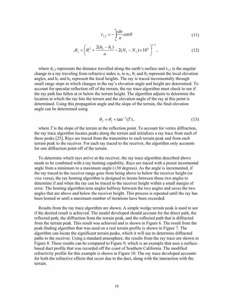
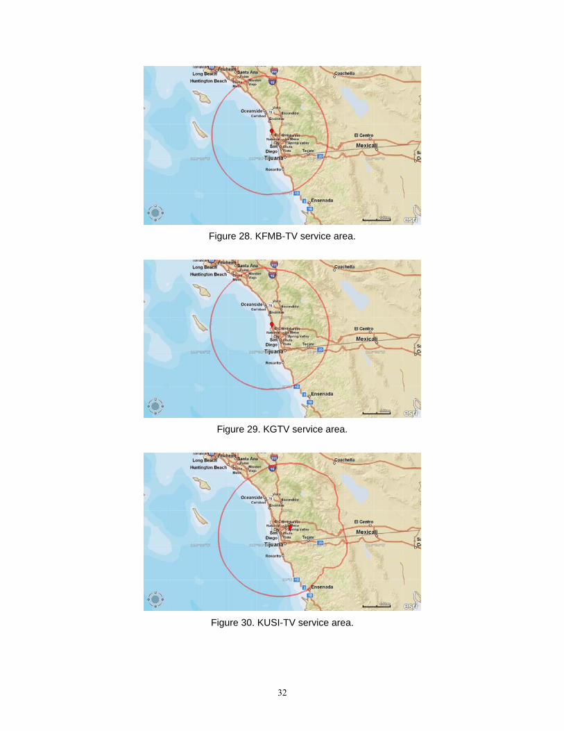
The third proposed set of test paths will use of DTV signals at various locations within San Diego County. Table 2 shows current over-the-air stations available in the San Diego area. Figures 28–33 show the service areas for each of the stations. These stations will provide data in the VHF/ultra high frequency (UHF) range over paths in excess of 80 km, which should be affected by surfaced-based ducts at the time of testing.

Table 2. DTV stations in the San Diego area.

DTV Tower Site Frequency (MHz) Transmitter (kW) Antenna Height (m AGL) KFMB-TV 180–186 14.87 75.7 KGTV 192–198 20.7 68 KUSI-TV 494–500 355 52 KSWB-TV 500–506 322.8 55.2 KPBS 566–572 350 50.9 KNSD 626–632 370 37

32

Figure 28. KFMB-TV service area.

Figure 29. KGTV service area.

Figure 30. KUSI-TV service area.

33

Figure 31. KSWB-TV service area.

Figure 32. KPBS service area.

Figure 33. KNSD service area.

35

4. CONCLUSIONS

Evaluating the performance claims of wideband communication systems will require a RF channel model that arises from the Navy’s needs. U.S. Navy shipboard systems contend with surface and evaporation ducts, which create complex propagation environments that can significantly impact system performance. The work developed under this effort is an automated model that can characterize the effect of anomalous propagation conditions on system performance. The limitations of this model need to be understood so that users can determine the applicability of this model for their needs. Future work for this project includes developing and optimizing the automated model and validating the model based on comparisons to other deterministic models along with a comparison to experimental data. The work presented in this document shows the theory that was used to develop an automated channel model that will be validated in the second year of the effort. The design of a wideband channel sounder was presented and the channel sounder will be used to collect a unique set of channel measurements over long-range paths. The experimental validation test plan was developed and measurements will be collected during the second year of this effort.

37

5. REFERENCES [1] V. Gadwal and A. Barrios. 2009. “Channel Modeling Using the Parabolic Equation for RF Communications.” Proc. of IEEE Military Communications Conference (MILCOM 2009) (pp. 18–21), Boston, MA. [2] A. Barrios. 1992.“Parabolic Equation Modeling in Horizontally Inhomogeneous Environments,” IEEE Trans. Antennas and Propagation, vol. 40, no. 7 (July), pp. 791–797. [3] A. Barrios. 1994. “A Terrain Parabolic Equation Model for Propagation in the Tropo-sphere,” IEEE Trans. Antennas and Propagation, vol. 42, no. 1 (January), pp. 90–98. [4] A. Barrios, K. Anderson, and G. Lindem. 2006. “Low Altitude Propagation Effects - A Validation Study of the Advanced Propagation Model (APM) for Mobile Radio Applications,” IEEE Trans. Antennas and Propagation, vol. 54, no. 10 (October), pp. 2869–2877. [5] A. Barrios. 1995.”Terrain and Refractivity Effects in a Coastal Environment: Results from the VOCAR Experiment,” 11th Annual Review of Progress in Applied Computational Electromagnetics, pp. 784–789, 20–25 March, [6] E. Salgado, V. Gadwal, J. Heger, B. Hobson, and D. Devasirvatham. 2008. “RF Coverage Verification issues in Public Safety Communications,” Proc. of IEEE Military Communications Conference (MILCOM 2008), 16–19 November, San Diego, CA. [7] Global Mobile Information Systems. 1999. “Report on Propagation Measurements for Variable Height Receive Antennas,” SSC San Diego – Signal Processing and Communication Technology Branch/SAIC, San Diego, CA. [8] A. Molisch. 2005. Wireless Communications, 1st Edition. Wiley-IEEE Press, London, UK. [9] R. Prasad. 22004. “OFDM for Wireless Communications Systems,” 1st Edition. Artech House, London, UK.. [10] R. Cooper and D. Stancil. 2009. “Improved Channel Sounding using Zero Correlation Zone Sequences,” Proc. of IEEE Global Communications Conference (GLOBECOM 2009), 30 November – 4 December, Honolulu, HI. [11] G. Simon and J. Schoukens. 2000.“Robust Broadband Periodic Excitation Design,” IEEE Trans. Instrumentation and Measurement, vol. 49, no. 2 (April), pp. 270–274.

38

[12] J. Austin, W. Ditmar, W. Lam, E. Vilar, and K. Wan. 1997. “A Spread Spectrum Communications Channel Sounder,” IEEE Trans. Communications, vol. 45, no. 7 (July), pp. 840–847. [13] R. Thoma, D. Hampicke, A. Richter, G. Sommerkorn, A. Schneider, U. Trautwein, and W. Wirnitzer. 2000. “Identification of Time-variant Directional Mobile Radio Channels,” IEEE Trans. Instrumentation and Measurement, vol. 49, no. 2 (April), pp. 357–364. [14] J. Liu, X. Zhou, and Y. Peng. 2001. “Spectral Arrangement and Other Topics in First-order Bandpass Sampling Theory,” IEEE Trans. Signal Processing, vol. 49, no. 6 pp. 1260–1263. [15] R. Luebbers, W. Foose, and G. Reyner. 1989. “Comparison of GTD Propagation Model Wide-Band Path Loss Simulation with Measurements,” IEEE Trans. Antennas and Propagation, vol. 37, no. 4 (April), pp. 499–505. [16] K. Wu, J. Schuster, R. Ohs, and R. Luebbers. 2004. “Application of Moving Window FDTD to Modeling the Effects of Atmospheric Variations and Foliage on Radio Wave Propagation over Terrain,” Proc. of IEEE Military Communications Conference (MILCOM 2004), 31 October - 3 November, Monterey, CA. [17] SSC Pacific. 2009. “User Manual for Advanced Refractive Effects Prediction System,” Atmospheric Propagation Branch, San Diego, CA. [18] K. Anderson and R. Paulus. 2000.“Rough Evaporation Duct (RED) Experiment,” Proc. of the Battlespace Atmospherics and Cloud Impact on Military Operations (BACIMO 2000), 25–27 April, Fort Collins, CA.. [19] A. Kukushkin. 2004. Radio Wave Propagation in the Marine Boundary Layer, 1st ed. Wiley-VCH Press, Germany. [20] G. Hufford and D. Ebaugh. 1985. “A Study of Interference Fields in a Ducting Environment,” Institute for Telcommunication Sciences, Rep. TR-85-177 (June), Boulder, CO. [21] ATSC Digital Television Standard. 2007 ATSC Document A/53 Part 2, 3 (January)

[22] D. Donohue and J. R. Kuttler. 2000. ”Propagation Modeling Over Terrain Using the Parabolic Wave Equation,” IEEE Transactions on Antennas and Propagation. [23] B. R. Bean and E. J. Dutton. 1966. Radio Meteorology, Central Radio Propagation Laboratory, National Bureau of Standards.

39

[24] F. J. Ryan. 1989. RPE: “A Parabolic Equation Radio Assessment Model,” AGARD Conference Proceedings No.453: Operational Decision Aids for Exploiting or Mitigating Electromagnetic Propagation Effects, 1989. [25] J. B. Keller. 1962. "Geometrical Theory of Diffraction,” J. Opt. Soc. Amer., vol. 52 (February).

41

6. BIBLIOGRAPHY [1] A. E. Barrios. 2003. “Considerations in the Development of the Advanced Propagation Model (APM) for the U.S. Navy Applications,” IEEE Proceedings of the International Radar Conference, pp. 77–82. [2] M. Levy. 2000. “Parabolic Equation Methods for Electromagnetic Wave Propagation,” The Institute of Electrical Engineers. [3] M. Le Palud. 2001.“Terrestrial Wireless Channel Modeling,” Communications for Network-Centric Operations: Creating the Information Force, MILCOM, vol. 2, pp. 1270–1274. [4] K. H. Craig and M. F. Levy.1989. “Field Strength Forecasting with the Parabolic Equation: Wideband Applications,” International Conference on Antennas and Propagation (April), pp. 461–465. [5] D. F. Gingras and P. Gerstoft. 1997. “The Effect of Propagation on Wideband DS-CDMA Systems in the Suburban Environment,” The First IEEE Signal Processing Workshop on Signal Processing Advances in Wireless Communications, pp. 333–336.

5f. WORK UNIT NUMBER

REPORT DOCUMENTATION PAGEForm Approved

OMB No. 0704-01-0188

The public reporting burden for this collection of information is estimated to average 1 hour per response, including the time for reviewing instructions, searching existing data sources, gathering and maintaining the data needed, and completing and reviewing the collection of information. Send comments regarding this burden estimate or any other aspect of this collection of information, including suggestions for reducing the burden to Department of Defense, Washington Headquarters Services Directorate for Information Operations and Reports (0704-0188), 1215 Jefferson Davis Highway, Suite 1204, Arlington VA 22202-4302. Respondents should be aware that notwithstanding any other provision of law, no person shall be subject to any penalty for failing to comply with a collection of information if it does not display a currently valid OMB control number. PLEASE DO NOT RETURN YOUR FORM TO THE ABOVE ADDRESS.

1. REPORT DATE (DD-MM-YYYY) 2. REPORT TYPE 3. DATES COVERED (From - To)

4. TITLE AND SUBTITLE 5a. CONTRACT NUMBER

5b. GRANT NUMBER

5c. PROGRAM ELEMENT NUMBER

5d. PROJECT NUMBER

5e. TASK NUMBER

6. AUTHORS

7. PERFORMING ORGANIZATION NAME(S) AND ADDRESS(ES) 8. PERFORMING ORGANIZATION REPORT NUMBER

10. SPONSOR/MONITOR’S ACRONYM(S)

11. SPONSOR/MONITOR’S REPORT NUMBER(S)

9. SPONSORING/MONITORING AGENCY NAME(S) AND ADDRESS(ES)

12. DISTRIBUTION/AVAILABILITY STATEMENT

13. SUPPLEMENTARY NOTES

14. ABSTRACT

15. SUBJECT TERMS

16. SECURITY CLASSIFICATION OF: a. REPORT b. ABSTRACT c. THIS PAGE

17. LIMITATION OF ABSTRACT

18. NUMBER OF PAGES

19a. NAME OF RESPONSIBLE PERSON

19B. TELEPHONE NUMBER (Include area code)

Standard Form 298 (Rev. 8/98)Prescribed by ANSI Std. Z39.18

April 2013 Final

Wideband Channel Modeling in Real Atmospheric Environments with Experimental Evaluation

V. M. Gadwal D. J. Belanger A. E. Barrios S. Ramlall B. C. Hobson

SSC Pacific 5622 Hull Street San Diego, CA 92152–5001

TD 3267

Dr. Syed Shah, Director, Research & Engineering (DR&E)/ Deputy Undersecretary of Defense DUSD(S&T) 1777 N. Kent Street, Suite 9030 Rosslyn, VA 22209

Approved for public release.

This is work of the United States Government and therefore is not copyrighted. This work may be copied and disseminated without restriction.

Evaluating the performance claims of wideband communication systems will require a RF channel model that arises from the Navy’s needs. U.S. Navy shipboard systems contend with surface and evaporation ducts, which create complex propagation environments that can significantly impact system performance. The work developed under this effort is an automated model that can characterize the effect of anomalous propagation conditions on system performance. The limitations of this model need to be understood so that users can determine the applicability of this model for their needs. Future work for this project includes developing and optimizing the automated model and validating the model based on comparisons to other deterministic models along with a comparison to experimental data. The work presented in this document shows the theory that was used to develop an automated channel model that will be validated in the second year of the effort. The design of a wideband channel sounder was presented and the channel sounder will be used to collect a unique set of channel measurements over long-range paths. The experimental validation test plan was developed and measurements will be collected during the second year of this effort.

Advanced propagation model boundary shift method wideband measurement system wideband channel model phased shift method maximum length sequences wideband parabolic equation model fixed grid method zero correlation zone sequence

V. M. Gadwal

U U U U 52 (619) 553-7663

INITIAL DISTRIBUTION

84300 Library (2) 85300 Archive/Stock (1) 55280 V. M. Gadwal (1)

Defense Technical Information Center Fort Belvoir, VA 22060–6218 (1)

Approved for public release.

SSC Pacific San Diego, CA 92152-5001