Who Will Feed China in the 21st Century? Income Growth and Food Demand

and Supply in China1

Emiko Fukase and Will Martin

29 September 2014

Abstract This paper uses resource-based cereal equivalent measures to explore the evolution of China’s demand and supply for food. Although demand for food calories is probably close to its peak level in China, the ongoing dietary shift to animal-based foods, induced by income growth, is likely to impose considerable pressure on agricultural resources. Estimating the relationship between income growth and food demand with data from a wide range of countries, China’s demand growth appears to have been broadly similar to the global trend. On the supply side, output of food depends strongly on the productivity growth associated with income growth and on the country’s agricultural land endowment, with China appearing to be an out-performer. The analyses of income-consumption-production dynamics suggest that China’s current income level falls in the range where consumption growth outstrips production growth, but that the gap is likely to begin to decline as China’s population growth and dietary transition slow down. Continued agricultural productivity growth through further investment in research and development, and expansion in farm size and increased mechanization, as well as sustainable management of agricultural resources, are vital for ensuring that it is primarily China that will feed China in the 21st century.

JEL Codes: Q11, Q17, Q18.

Keywords: cereal equivalents, China, food self-sufficiency, livestock, income growth

1 We would like to thank Ulrich K. H. M. Schmitt for the opportunity to prepare this paper for China’s Urbanization and Food Security project and for his guidance; Norman Rask and Kolleen Rask for their detailed advice on replicating and understanding the cereal equivalent measure of food and their comments; the participants in a conference held in Beijing in November, 2013, particularly Jikun Huang and Jun Yang, and those in the Agricultural Economics Society Annual Conference in Paris in April, 2014 and in a seminar at the University of Bordeaux the same month for very useful comments and discussions. We are also indebted to Luc Christiaensen, Mimako Kobayashi and Jonathan Nelson for their comments and suggestions. Any remaining errors are ours.

2

Who Will Feed China in the 21st Century? Income Growth and Food Demand and Supply in China

1. Introduction  

The balance between domestic supply and demand for food in China is extremely important both

for China and for the world. Since China embarked on its economic reforms in 1978, it has had

dramatic increases in income, achieving an 8.5 percent average annual per capita Gross

Domestic Product (GDP) growth rate in purchasing power parity (PPP) terms (the World

Development Indicators (WDI), the World Bank).

This rapid economic growth has contributed greatly to changes in Chinese diets both in

quantity and in composition. Since China’s overall per capita calorie consumption levels already

appear to be well above world average levels, and to be approaching the level in the Republic of

Korea, China’s per capita food consumption in caloric terms seems unlikely to rise dramatically.

However, diets in China are likely to change in composition, as consumers shift their diets

increasingly from crop based to animal based products and away from basic staples. The shift to

the diets of more affluent consumers imposes greater burdens on the agricultural sector since the

production of animal based food takes much greater amounts of agricultural resources and

generates more environmental externalities than production of a vegetable-based diet (Steinfeld,

Gerber, Wassenaar, Castel, Rosales and De Haan, 2006; Rask and Rask, 2011).

Since the commencement of its reforms, China has experienced an impressive

agricultural output growth, with its agricultural GDP at constant prices growing at an annual rate

of 4.6 percent between 1978 and 2011, four times faster than the rate of population growth

(Huang, Rozelle and Yang, 2013). The introduction of the Household Responsibility System

(HRS) (1978), in which farmers were allowed to lease land from the collectives and to exercise

autonomy in their production decisions, gave incentives to farmers to increase their productivity

3

and created a foundation for family-based farming. Since then, China has sustained its output

growth, largely benefiting from growing agricultural Research and Development (R&D)

investment and high use of key inputs such as fertilizer and irrigation systems.2 However, in

recent years, China’s demand for food appears to have been growing more quickly than its

supply. As a result, China’s trade position for food has turned from surplus to deficit, and this

gap has been widening (Fukase and Martin, forthcoming). Some concerns about China’s food

self-sufficiency have arisen among Chinese policy makers and other stakeholders, especially

since China is relatively poorly endowed with agricultural land and water supplies compared to

its population base.3

A World Bank project on urbanization and food security has recently devoted a great deal

of research to the question of China’s food demand and supply. This research looks in detail at

key issues such as the impact of urbanization on China’s food self-sufficiency and food security

(Huang et al., 2013), on land availability (Deng, Huang and Rozelle, 2013) and on water

availability (Wang, Huang and Rozelle, 2013). Using detailed structural models built up from

estimated parameters of demand systems and production structures for China, Huang et al.’s

study (2013) predicts that China will need to import feed grains and some other foods for some

time but that its overall food self-sufficiency is likely to remain at above 90 percent level through

2030. Their results are consistent with those obtained from other studies, for instance, the

forecast for China by 2022 prepared by OECD/FAO (2013) and a recent study using a multi-

country multi-sector applied general equilibrium model (Anderson and Strutt, 2013).4

2 Since the economic reforms, China has sustained an impressive annual growth rate in agricultural total factor productivity (TFP) of over 2 percent (Huang et al., 2013). 3 China has about 20 percent of the world’s population and 35 percent of its agricultural labor force, but has only 11 percent of the world’s agricultural land and less than 6 percent of its water resources (Christiaensen, 2012). 4 Using the Global Trade Analysis Project (GTAP) model, Anderson and Strutt (2013) project that China’s agricultural self-sufficiency rate may fall about ten percentage points from the baseline level of 97 percent by 2030.

4

The purpose of this paper is to analyze China’s income-consumption-production

dynamics for food using an entirely different approach to those used in the studies cited above—

econometric techniques based on data for 154 countries during the period 1980-2009. The paper

aggregates both the demand for and the supply of food into resource based cereal equivalents

(Yotopoulos, 1985; Rask and Rask, 2004, 2011). This approach takes into account one of the

central features of food demand behavior—the shift from reliance on direct consumption of

grains and other sources of basic carbohydrates into a more diversified diet including edible oils

and protein-rich animal products as incomes grow. On the supply side, agricultural output is

specified as a function of income and land endowment, with agricultural output growing in

response to the productivity growth that is associated with national output growth per person.

The econometric approach used relies on the experiences of a wide range of countries and is

intended to complement, rather than replace, more detailed country-specific structural

approaches.

Section 2 analyzes the changes that have occurred in dietary patterns in China. Section 3

presents the methodology used for the analysis and implements regression analyses. We first

discuss the construction of the cereal equivalent measure of food output and demand. Next, we

replicate and extend the income-consumption analysis of Rask and Rask (2004, 2011) to the

period 1980-2009. Then, we modify Rask and Rask’s approach on the production side,

specifying a regression model relating both income and land endowment to production. Finally,

we suggest the implications of these trends for China’s likely net import demands in the future.

Section 4 presents conclusions.

 

5

2.  Changing  Patterns  of  Chinese  Diets  

Since China embarked on its market-oriented reforms in 1978, it has achieved dramatic

economic growth. China’s per capita GDP in PPP 2005 prices, which was $524 in 1980, grew at

an average annual growth rate of 8.5 percent to reach $7,958 in 2012 (the WDI, the World

Bank). This rapid economic growth appears to have contributed greatly to changes in Chinese

diets both in quantity and in composition.

Figures 1a-c show estimated average daily calorie, protein and fat intake per capita for

China and selected countries for the period 1980-2009. Total calorie, protein and fat intakes are

further decomposed into those sourced from crop and animal products. Figure 1a shows that total

calorie intake per person per day in China grew substantially, from 2,163 kcal in 1980 to 3,036

kcal in 2009. The decomposition of the source of this change reveals that a majority of the

increase comes from a rise in the consumption of animal products, while the calorie intake from

crops grew slowly and stabilized at around 2,300 kcal in recent years. China’s increase in per

capita calorie intake has been much faster than the world average, which grew 2,490 kcal in 1980

to 2,831 kcal in 2009. As of 2009, China’s calorie intake was approaching the level in the

Republic of Korea, although it remained lower than levels observed in the United States and the

European Union (EU) countries. Figure 1a also shows that the total average individual annual

calorie intake among high income countries, namely, the United States, Japan and EU countries,

declined somewhat in the most recent years.

Figure 1b shows that protein intake in China nearly doubled from 54 g per capita in 1980

to 94 g per capita in 2009 and that about three quarters of this growth came from consumption of

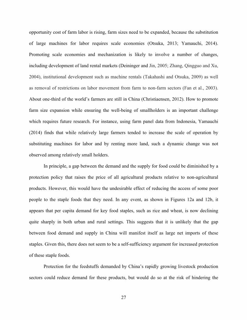
animal products. Figure 1c shows that fat intake in China nearly tripled from 34 g per capita in

6

1980 to 96 g per capita in 2009, and that about two thirds of this growth came from increases in

animal product consumption.

The changing dynamics of food consumption shown above affect supply and demand

balances for food directly and indirectly. In particular, whereas direct demand for food grains

such as wheat and rice, tends to decrease as income rises, the same driving force (the rise in per

capita income) is likely to lead to an increase in indirect demand for feed grains as more grain

and other feeds are needed for animal production. Figure 2a shows the self-sufficiency ratios for

the key staple foods (rice, wheat, maize and soybeans combined) for the period 1960-2012 for

Asian countries. Most strikingly, the self-sufficiency ratios declined sharply in higher income

Asian countries, from around 75 to 27 percent for Japan, from about 88 to 21 percent for the

Republic of Korea and from about 86 to 13 percent for Taiwan, China, during the period

1960/1961-2012/2013 (Production, Supply and Distribution (PSD) data, the United States

Department of Agriculture (USDA)).5 Figure 2a also shows that whereas China tended to

achieve self-sufficiency for grains for the 1960s, 1970s, 1980s and most of the 1990s, its self-

sufficiency ratio has been declining in recent years.

Figure 2b reports the evolution of the demand and supply gap by major grains for China.

It is clear that China’s recent declining self-sufficiency ratio for grains is predominantly

attributable to a large increase in soybean imports. The expansion of the livestock sector which

increased the demand for protein meal, along with the rise in consumers’ demand for vegetable

oils, was a major factor leading to the growing demand.6 The Chinese government appears to

5 However, further disaggregation of the data reveals that the self-sufficiency ratios for Japan, the Republic of Korea and Taiwan, China, vary by grain: whereas imports of corn contributed most to the widening gap for three countries, they have been relatively self-sufficient in terms of rice. 6 In 2009, out of 59 million tons of domestic soybean consumption, about 9 million tons was consumed as food. 49 million tons of soybean was crushed and made into 9 million tons of vegetable oil and 39 million tons of soymeal (PSD, USDA).

7

have responded to the rising demand by liberalizing soybean imports gradually (Weiming and

Ying, 2013).7

Some scholars view China’s increasing imports of soybeans as a rational response to the

rising resource constraints in China, especially because soybean is a crop which requires a large

amount of land and water (Christiansen, 2012; Qiang, Liu, Cheng, Kastner and Xie, 2013;

Weiming and Ying, 2013). For instance, calculating the “virtual” land use embodied in China’s

imports and exports of crops, Qiang et al. (2013) find that China has become a massive net

importer in terms of virtual land during the period 1986-2009 and that the increase in virtual land

imports was mainly driven by the rise in imports of soybean. By effectively   freeing   land, the

soybean imports appear to have saved China’s domestic cropland area for food grains such as

wheat and rice which   tend   to  be   regarded  as  more   important   for   food   security  objectives  

(OECD   and   FAO,   2013;   Qiang   et   al.,   2013).   In   terms   of   virtual   water   trade,   Chapagain,

Hoekstra and Savenije (2006) and Hoekstra and Hung (2005) find that China conserved its

national  water  resources  by importing water-intensive agricultural products.

3. Methodology  and  Regression  Analyses  

As incomes grow, consumers diversify their food consumption away from basic food staples.

This process includes a move to include more edible oils, vegetables, fruit and animal products.

Per capita consumption of staple foods declines during this process. Historically, the

urbanization process that is inextricably linked with income growth appears to have reduced per

capita food consumption slightly by reducing energy needs (Clark, Huberman and Lindert 1995).

In Asia, it also appears to have increased demand for wheat relative to rice (Huang and David

7 China adopted a more liberal trade scheme for soybeans in 1996 which was locked in through negotiations to access the World Trade Organization (WTO) (Weiming and Ying, 2013). China became a full member of the WTO in 2001.

8

1993). However, it now appears that the key driving force behind changes in per capita food

consumption is changes in real incomes—the same increases in real incomes that drive the

urbanization process (Satterthwaite, McGranahan and Tacoli 2010).

3.1. Cereal Equivalent (CE) Measures of Food  

Some scholars argue that the dietary shift from crop based to animal based products may

increase total food demand sharply relative to supply, due to the inefficient conversion of plant

based feeds (typically cereals8) into animal based foods.9 Yotopoulos (1985) argues that the

supply of cereals available for food may decline as developed and middle-income countries

consume cereals disproportionately as feed, raising world prices of cereals. He suggested that

this “Food-Feed Competition” may have contributed to the world food crisis of 1972-74. More

recently, a number of scholars have explored the implications of this dietary shift on agricultural

resources and the environment (e.g., Elferink and Nonhebel, 2007; Garnet, 2009; Gerbens-

Leenes, Nonhebel and Ivens, 2002ab; Gerber, Steinfeld, Henderson, Mottet, Opio, Dijkman,

Falcucci and Tempio, 2013; Steinfeld et al. 2006; Williams, Audsley and Sandars, 2006;

Wirsenius, 2003; Wirsenius, Azar and Berndes, 2010). For instance, Wirsenius (2003) argues

that the idea of competition for grains between animals and humans does not capture fully the

resource implications of dietary change, since the core issue is the competition for land rather

than competition for consumption of cereals. Analyzing comprehensively total feed10 and land

requirements in their land-minimizing model, Wirsenius et al. (2010) suggest that greater feed-

8 About 34 percent of cereals were consumed indirectly in the form of animal feed in 2009 (FAOSTAT). 9 Yotopoulos (1985) suggests calorie-equivalent grain-meat conversion ratios vary from 2:1 for poultry to 7:1 for grain-fed beef, estimates that do not appear to take into account indirect use, such as for breeding animals, considered by Rask and Rask (2011). 10 In addition to the edible-type crops (e.g., cereals, starchy roots, sugar crops and oil crops), Wirsenius (2003) considers other types of feeds such as the use of forage crops, pastures, and by-products/residues.

9

to-food efficiency in animal production, decreased food wastage and dietary changes towards

less land-demanding foods would help to reduce agricultural land use.  

Animal production competes for land directly, for instance, for grazing and fattening,

and indirectly through the need to produce animal feeds.11 Gerbens-Leenes et al. (2002ab) show

that foods associated with affluent lifestyles, especially animal products, oils and fats, and

beverages, tend to require more land for their production than foods associated with less affluent

lifestyles. For China, following Gerbens-Leenes et al. (2002ab)’s methodology, Li et al. (2013)

find that China’s urbanization appears to have increased pressure on limited arable land

resources, since urban residents consume more animal based and other land-demanding food

than their rural counterparts.

The approach adopted in this paper is based on the methodology developed by Rask and

Rask (2004, 2011) which converts crop and animal products into cereal equivalents. The CE

coefficients for crop-based products are computed very simply by matching their caloric content

to those of an equal weight of cereals, assuming broadly similar efficiencies across commodities

but taking into account the greater resource use associated with producing foods that contain

more calories per unit of weight (e.g., vegetable oils) relative to those that have, for instance, a

higher water content (e.g., starchy roots). For animal products, the CE coefficients reflect the

feedstuff used to produce one unit of animal products in terms of the dietary energy equivalent of

a unit of corn, considering not only grains consumed but also other types of feed such as protein

supplements, forages (including pasture) and other feeds.12

11 Livestock is the world’s largest user of land resources, with grazing land and cropland dedicated to the production of feed crops and fodder representing about 70 percent of all agricultural land. About 33 percent of arable land is used to produce livestock feed (Steinfeld et al., 2006). 12 The CE coefficients developed by Rask and Rask (2004, 2011) are based on a study published by the USDA (1975). The USDA study is unique in covering all types of feeds including forage crops and pasture in calorie equivalents of corn over the period 1964-1973. Wirsenius (2003) challenges the view that the use of non-edible feeds is “free” arguing that it involves opportunity costs such as production of feedstock for biofuels, preservation of

10

Table 1 shows the CE coefficients used to convert crop and animal products into cereal

equivalents.

Table 1. Sample Cereal Equivalent (CE) Coefficients Crop products Animal productsa

Products Coefficients Products Coefficients Cereals 1.00 Bovine meat 19.8 Fruits 0.14 Pig meat 8.5 Pulses 1.06 Poultry meat 4.7 Starchy roots 0.25 Mutton & Goat meat 19.8 Sugar, sweeteners 1.08 Eggs 3.8 Tree nuts 0.74 Milk 1.2 Vegetable oils 2.73 Vegetables 0.07

Source: Rask and Rask (2011) and authors’ calculation. aMeat coefficients represent animal carcass weight to conform with FAOSTAT definition of meat consumption.

The coefficients in Table 1 reflect the high resource costs of producing animal products

relative to cereals, and illustrate the great differences among animal products. The CE coefficient

of 19.8 for carcass beef, for instance, takes into account the large amount of feed used directly to

produce beef; the relatively low dressing weight percentage for live cattle (0.59); and feed for

breeding cows and young calves needed to supply production animals and replacement breeding

stock.13 Pork, poultry and fish are more efficient both because of generally higher feeding

efficiencies and the lower costs involved in maintaining their breeding stock. Within crop

products, CE coefficients range from 2.7 for vegetable oils to 0.07 for vegetables.

The magnitudes of the CE coefficients appear to be broadly consistent with other

estimates of land requirements in the literature (e.g., Gerbens-Leenes et al. 2002ab, Williams et

favorable soil condition and restoration of ecosystems and habitats. Wirsenius et al. (2010) show that the global use of the non-edible type feeds is substantial. 13 Using beef as an example, Rask and Rask (2011) use a feed conversion ratio of 11.7 for producing live cattle, taking into account feed for both animals slaughtered and for breeding animals. This figure is converted to carcass weight using a dressing weight percentage of 59 percent, which gives rise to the final value of 19.8 (11.7/0.59). Carcass weight is used in order to conform to FAOSTAT meat consumption coefficients which are presented in carcass weight format (e-mail communication with Norman Rask).

11

al., 2006, Wirsenius, 2003, 2010). For instance, using data for the Netherlands in 1990, Gerbens-

Leenes et al. (2002a) estimate the land requirement for beef to be 20.9 m2 year per kilogram of

meat which is more than twice that for pork (8.9 m2 year per kilogram of meat) whereas their

land requirement estimate for cereals turns out to be relatively small (1.4 m2 year per kilogram).

For China, land requirement estimates obtained by Li et al. (2013) and Zhen et al. (2010) are

broadly comparable with those from other studies.14 The implications for environmental burdens

implied by the CE coefficients15 are also generally in line with the findings of other studies.16

Researchers tend to find that beef production has the most severe GHG impact per kilogram of

meat, followed by pork and chicken production (e.g., Fiala, 2008; Gerber et al., 2013; Steinfeld

et al., 2006).

Finally, the cereal equivalent measure used in this study does not consider varying feed

requirements for animal production depending on technology (e.g., feed mix and efficiencies),

production systems (Robinson, Thornton, Franceschini, Kruska, Chiozza, Notenbaert and You,

2011) and local resource availabilities. Differentiating CE coefficients by regions and by

production systems would be a potential subject of future research. Further, our analytical

technique in the empirical section does not take into account distortions from agricultural

incentives, food price policy, or farm gate pricing differences related to product self-sufficiency.

14 For instance, the arable land requirement for beef of 2.5 m2 per kilogram of meat estimated by Li et al. (2013) is much smaller than that of Zhen et al. (2010) of 16.7 m2 per kilogram, largely reflecting the fact that the former study considers only the arable land area for growing “refined” livestock feed (e.g., maize etc.) whereas the latter study includes grassland used to grow grass fodder. 15 For instance, Williams et al. (2006) find the global warming potential to be about 20 times higher for beef production than for wheat production (Rask and Rask, 2011; Williams et al., 2006). 16 Livestock production is believed to be one of the largest sources of greenhouse gases (GHG), contributing about 18 percent of the environmental pressures that are believed to be causing global warming (Gerber et al., 2013; Steinfeld et al., 2006). Feed production and processing, and enteric fermentation from ruminants are reported to be the two main sources of emissions, representing 45 and 39 percent of the sector emissions respectively, followed by manure storage and processing (10 percent) (Gerber et al., 2013). For instance, it is reported that, in the Brazilian Amazonian region, a significant amount of carbon dioxide is released when forest is converted into grazing for cattle ranching or into arable land for soy production (Garnett, 2009; Steinfeld et al., 2006). Brazil has committed to a range of mitigation targets to reduce deforestation in the Amazon and in the Cerrado (Gerber et al., 2013).

12

It would be desirable to do this in future work, but we believe that the impacts on the aggregate

measures that we consider are likely to be less than protection rates might suggest. Countries

with high average rates of agricultural protection typically provide high rates of protection on

traditional staple foods such as rice. But political economy pressures generally keep the rate of

protection on feedgrains quite low and hence keep the prices of domestically-produced livestock

products like pork and poultry low relative to staple grains. This structure of protection results in

an incentive for consumers to increase their consumption of livestock products, thus accelerating

the dietary transition that is the focus of this study.

3.2. Estimating Consumption Demand

Cereal Equivalent (CE) Consumption in China

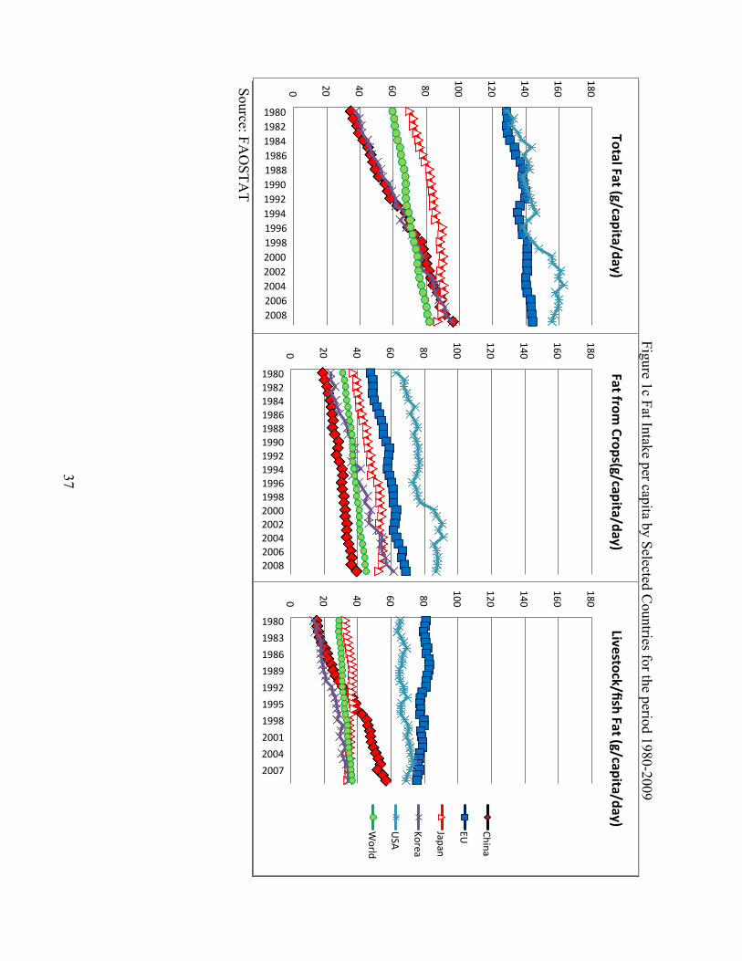
Figure 3a shows that China’s CE consumption expanded nearly four times from 407 million tons

in 1980 to 1,479 million tons in 2009 (a 264 percent increase). Figure 3a also shows that the rise

is mainly driven by the increase in consumption of animal products (which accounts for 87

percent of the change in consumption), while CE consumption of crops remains relatively

steady, contributing the remaining 13 percent of CE food consumption increases since 1980.

The increase in China’s food consumption at the national level is attributable to both

population growth and diet upgrading. Figure 3b shows that China’s population increased from

1.0 billion in 1980 to 1.4 billion in 2009 and that its population growth is expected to taper off

gradually. Figure 3c decomposes the change in CE consumption into the components of

population growth17 and of diet changes since 1980. The figure shows that about one-third of the

increase in food consumption is attributable to China’s population growth, and the remaining

17 The population growth component reflects both the increase in population and the share of dietary changes imputed to the added population.

13

two-thirds can be explained by the change in diets. As China’s population growth is slowing and

its total population is projected to peak around the year 2025 (at a level about 2.3 percent higher

than in 2014) (FAOSTAT), the primary driver of food consumption increases is likely to be

change in diet, and therefore change in per capita consumption.

Income-Consumption Relationship: Regression Analyses

While we can observe the rapid growth in China’s consumption of food over the period since

1980, this gives us little insight into the way this growth is likely to play out in the future. To

gain some insights into this, we turned to econometric analysis using a large sample of countries.

This allows us to view a much larger range of real incomes and to obtain a better idea of the

extent to which the growth of food consumption in cereal equivalents begins to decelerate. This

relationship includes most importantly the effects of income growth on the demand for basic

food staples and for foods with relatively high income elasticities but also other influences on

demand such as changes in the rate of assistance to agriculture with income growth (Anderson

1995).

We estimate the CE consumption-income relationship using the functional form used in

Rask and Rask (2004, 2011). Specifically,

y = ƒ(x) = A1 – A2𝑒!!" , ƒ' ˃0, ƒ''˂0 (1)

where y is CE consumption per capita and x is PPP GDP per capita in 2005 constant prices. As ƒ'

˃0, ƒ''˂0, this functional form captures the observed pattern of the change in CE consumption,

which rises more rapidly at early stages of development and tapers off at higher levels of income.  

It implies that, as incomes continue to increase, consumption asymptotically approaches a limit

given by A1. Historical figures for CE consumption per capita are calculated using food supply,

food demand and population data extracted from FAOSTAT. The GDP data at PPP are obtained

14

from the World Development Indicators (the World Bank). We use the data for the period 1980-

2009 since the GDP data are available only after 1980 and the latest data available in FAOSTAT

are for 2009.  

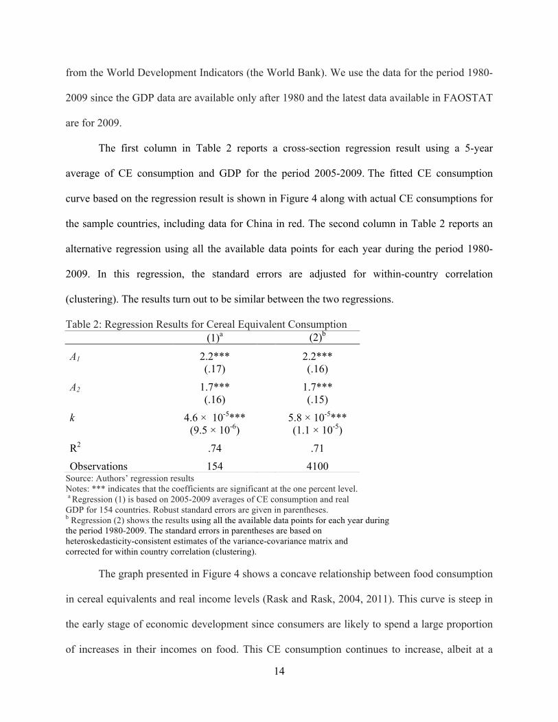
The first column in Table 2 reports a cross-section regression result using a 5-year

average of CE consumption and GDP for the period 2005-2009. The fitted CE consumption

curve based on the regression result is shown in Figure 4 along with actual CE consumptions for

the sample countries, including data for China in red. The second column in Table 2 reports an

alternative regression using all the available data points for each year during the period 1980-

2009. In this regression, the standard errors are adjusted for within-country correlation

(clustering). The results turn out to be similar between the two regressions.

Table 2: Regression Results for Cereal Equivalent Consumption

Source: Authors’ regression results Notes: *** indicates that the coefficients are significant at the one percent level. a Regression (1) is based on 2005-2009 averages of CE consumption and real GDP for 154 countries. Robust standard errors are given in parentheses. b Regression (2) shows the results using all the available data points for each year during the period 1980-2009. The standard errors in parentheses are based on heteroskedasticity-consistent estimates of the variance-covariance matrix and corrected for within country correlation (clustering).

The graph presented in Figure 4 shows a concave relationship between food consumption

in cereal equivalents and real income levels (Rask and Rask, 2004, 2011). This curve is steep in

the early stage of economic development since consumers are likely to spend a large proportion

of increases in their incomes on food. This CE consumption continues to increase, albeit at a

(1)a (2)b

A1

2.2*** (.17)

2.2*** (.16)

A2

1.7*** (.16)

1.7*** (.15)

k

4.6 × 10-5*** (9.5 × 10-6)

5.8 × 10-5*** (1.1 × 10-5)

R2 .74 .71 Observations 154 4100

15

slower rate, as incomes grow further and consumers substitute higher-order foods (such as

animal products) for cereals and tubers. Only at higher levels of income such as $40,000 per

person does per capita CE consumption growth slow down as the diet shift is nearing

completion. This graph also shows the income-consumption pairs for a large range of countries,

making clear that there is considerable variation around this broad trend. This is to be expected

with such a simple measure, given the differences in food consumption patterns among nations,

some of which may be due to inherent cultural features, with others perhaps related to habit

formation patterns of the type analyzed by Atkin (2013), or to food price differences related to

policy and product self-sufficiency.

Based on the FAO statistics that we use, China’s consumption pattern is close to the

average demand pattern for our global sample. Not surprisingly, consumption levels are

particularly high in countries such as Australia and Brazil, where beef and sheepmeats are

produced largely using pasture whose price is determined—given the available technology—by

the prices of these beef and sheep products, rather than by arbitrage between pasture and grain.

Japan is a negative outlier, probably because of the importance of seafood in its historical

animal-product diet with the price of fish determined—at least until recently—by costs of

catching from the wild, rather than by the costs associated with fish-farming. Only recently has

arbitrage between wild-caught and farm-raised seafood justified the use of our approach to

aggregation on the assumption that fish can be produced using cereal products.

In order to gain historical perspective, Figure 5 shows the changes in CE consumption

between the beginning of the sample period (the year 1980) and the end (the year 2009). This

shows that most countries where per capita income grew substantially observed a sizeable

increase in consumption levels, with the slope of the resulting ray being very broadly similar to

16

that of the estimated equation in the range relevant to the income growth of that country.

Contrasting cases, such as the decline in observed consumption levels in Australia, appear to

reflect structural shifts in demand away from meats such as beef and sheepmeats that rely on

relatively inefficient conversion processes into more efficiently-produced livestock products like

poultry (Martin and Porter 1985). The drop of CE consumption for Hungary appears to reflect

the transition from a high level diet, which was induced by low food prices and production

subsidies under a centrally planned low food price system, to a food price level more consistent

with market economies (Rask and Rask, 2004).

Figure 6 compares the estimated growth of demand for cereal equivalents and for calories

on a comparable scale. We use the same functional form (1) to estimate the relationship between

income growth and calorie consumption. China’s CE and calorie consumption points for each

year during the period 1980-2009 are also shown in the same figure. Figure 6 shows two results

that are significant for our analysis. First, consumption of calories tends to level off much earlier

and at a much lower level than consumption of cereal equivalents. Second, China’s per capita

consumption levels for both calories and cereal equivalents have been closely consistent with

global trends.

3.3 Production

Income, Productivity and Land Endowments

Agricultural output tends to rise as real income rises (see Figure 9 below). The primary driving

force for this relationship is the increase in productivity that contributes to increases in national

incomes. This relationship is, however, influenced by several other factors, including: (i) the

shift in demand away from staple foods, as discussed in the demand section, that influences the

17

prices of non-traded or incompletely-traded foods and hence the incentives for their production,

(ii) differentials in the rates of productivity growth between agriculture and other sectors (Martin

and Mitra, 2001), and (iii) Rybczynski effects when high (or low) rates of capital accumulation

change factor endowments (Martin and Warr, 1993) or when land use changes alter agricultural

land endowments. Since the growth rate of the agricultural sector is almost invariably slower

than that of the economy as a whole for most countries, we would generally expect a given

percentage change in GDP to result in a less-than-proportional increase in agricultural output.

In order to see if the data support a positive association between income and agricultural

productivity, Figures 7a and 7b plot the relationship between GDP and proxies for land and labor

productivity. The income-productivity pairs for China are shown in red. Figure 7a shows the

relationship between GDP PPP per capita and the average cereal yield per hectare as a proxy of

land productivity. Figure 7a confirms that income level and land productivity are positively

associated and that China achieved high land productivity relative to its current level of income,

almost approaching the productivity level reached by high performing Organization for

Economic Cooperation and Development (OECD) countries. This impressive achievement is

likely to reflect a number of factors, for instance, a high degree of fertilizer use, expansion of

irrigated land,18 widespread use of multiple-cropping and the introduction of new seed varieties

and other technology improvements (Huang and Rozelle, 1996).

Figure 7b plots the relationship between real GDP per capita and agricultural value added

per worker as an indicator of labor productivity. Not surprisingly, higher income is generally

associated with higher agricultural labor productivity. However, in contrast to China’s high land

productivity, its labor productivity is found to be very low given its level of development.

18 Christiaensen (2012) reports that fertilizer use intensity in China is amongst the highest in the world (Figure 6, p.17) and that yields were further boosted through expansion of irrigation (Figure 7, p.18).

18

China’s low labor productivity may possibly be attributable to small farm size (0.6 hectare on

average), land fragmentation (Jia and Petrick, 2013), and to the labor-intensive nature of family

based farming. In addition, several scholars report that the labor productivity gap between farm

and non-farm sectors remains high in China (e.g., Fan, Zhang and Robinson, 2003; Kujis and

Wang, 2006). Labor is likely to move out of agriculture and this shift is an inherent part of the

process of economic development (World Bank and the Development Research Centre (DRC) of

State Council, 2014).

Figure 8 and its attached table show the evolution of agricultural land endowments for

selected countries. Following Rask and Rask (2011), hectares of land per capita are computed as

a summation of arable land, land in permanent crops, and one-third of land in permanent pastures

using FAOSTAT data. Since 1980, the worldwide per capita amount of agricultural land has

decreased by about one third from 0.54 ha in 1980 to 0.39 ha in 2009, revealing a trend that

agricultural land per capita has been becoming increasingly scarce worldwide. China appears to

be a relatively land-scarce country, with its land endowment only about half the world average.

Not surprisingly, relatively large net exporters of food, such as Brazil and the United States, are

much better-endowed with agricultural land, having agricultural land endowments that are

roughly four and five times China’s. However, the United States has reduced its per capita

agricultural land by about a third over the same period. In comparison with neighboring net food

importing countries such as the Republic of Korea and Japan, China has nearly four times the

agricultural land endowment per person as the Republic of Korea and almost five times as much

as Japan.

19

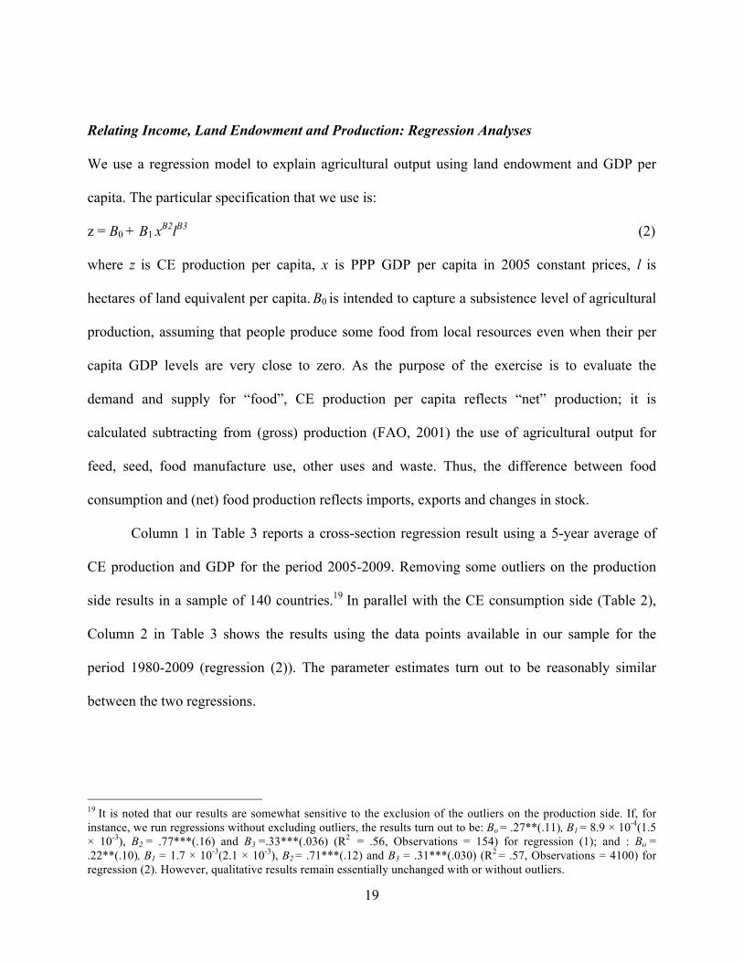
Relating Income, Land Endowment and Production: Regression Analyses

We use a regression model to explain agricultural output using land endowment and GDP per

capita. The particular specification that we use is:

z = B0 + B1 xB2lB3 (2)

where z is CE production per capita, x is PPP GDP per capita in 2005 constant prices, l is

hectares of land equivalent per capita. B0 is intended to capture a subsistence level of agricultural

production, assuming that people produce some food from local resources even when their per

capita GDP levels are very close to zero. As the purpose of the exercise is to evaluate the

demand and supply for “food”, CE production per capita reflects “net” production; it is

calculated subtracting from (gross) production (FAO, 2001) the use of agricultural output for

feed, seed, food manufacture use, other uses and waste. Thus, the difference between food

consumption and (net) food production reflects imports, exports and changes in stock.

Column 1 in Table 3 reports a cross-section regression result using a 5-year average of

CE production and GDP for the period 2005-2009. Removing some outliers on the production

side results in a sample of 140 countries.19 In parallel with the CE consumption side (Table 2),

Column 2 in Table 3 shows the results using the data points available in our sample for the

period 1980-2009 (regression (2)). The parameter estimates turn out to be reasonably similar

between the two regressions.

19 It is noted that our results are somewhat sensitive to the exclusion of the outliers on the production side. If, for instance, we run regressions without excluding outliers, the results turn out to be: Bo = .27**(.11), B1 = 8.9 × 10-4(1.5 × 10-3), B2 = .77***(.16) and B3 =.33***(.036) (R2 = .56, Observations = 154) for regression (1); and : Bo = .22**(.10), B1 = 1.7 × 10-3(2.1 × 10-3), B2 = .71***(.12) and B3 = .31***(.030) (R2 = .57, Observations = 4100) for regression (2). However, qualitative results remain essentially unchanged with or without outliers.

20

Table 3: Regression Results for Cereal Equivalent Production

Source: Authors’ regression results Notes: ** and *** indicate that the coefficients are significant at the five and one percent level respectively. a Regression (1) is based on 2005-2009 averages of CE consumption and real GDP for 140 countries. The robust standard errors are given in parentheses. b Regression (2) shows the results using all the available data points for each year during the period 1980-2009. The standard errors in parentheses are based on heteroskedasticity-consistent estimates of the variance-covariance matrix and corrected for within country correlation (clustering).

Based on the parameter values reported in column 1 in Table 3, Figure 9 shows the

estimated relationship between income levels and cereal equivalent production. To allow

comparison in two dimensions, the CE production schedule for each country is adjusted so that it

has the same land endowment as China (0.21 hectare per capita as an average of the period 1980-

2009 per person).20 The estimated CE production curve is visually close to linear: it rises in line

with income, although less rapidly than income because of the secular decline in agriculture’s

share of national income. From Figure 9, it appears that China has been an out-performer in

terms of output. Agricultural output, which is slightly below the consumption level, is

substantially above the global trend level. This may reflect the relatively high productivity of

much of China’s agricultural land and the extraordinary efforts made in China to increase

20 Both sides of equations (2) are divided by   !!

!.!"  .!!

where li is the average of land endowment of country i and 0.21 is the average land endowment of China.

(1)a (2)b

B0

.24** (.12)

.23** (.11)

B1

4.3 × 10-3 (5.4 × 10-3)

3.9 × 10-3 (4.3 × 10-3 )

B2

.60*** (.11)

.62*** (.10)

B3

.33*** (.031)

.32*** (.037)

R2 .64 .65 Observations 140 3762

21

productivity in recent decades (International Food Policy Research Institute (IFPRI), 2012; Jin,

Huang, Hu and Rozelle, 2002). For instance, a study by the IFPRI (2012) documents that more

than one-third of the increase in global public agricultural R&D spending between 2000 and

2008 was attributable to China.21 However, there have been some concerns expressed about

measurement problems with China’s livestock production, an issue that is discussed in more

detail in the Appendix.

3.4. Supply and Demand Balance for Food

Figures 10a-c compare how the historical patterns of CE production and consumption differ

depending on land endowments, translating the differences in endowments into differences in the

income response curves based on the parameter results reported in Table 3 (regression (2)).

Figure 10a plots actual CE production and consumption points for China for the period 1980-

2009 along with estimated global CE production and consumption trend curves. The global

production schedule is evaluated at China’s land endowment (0.21 hectare per person on

average). Figure 10a demonstrates the differing growth patterns of CE production and

consumption. At early stages of development, demand for food tends to grow faster than

production, widening the gap between supply and demand. As incomes grow, the growth of

consumption will slow down relative to growth of production and the gap will begin to close.

Figure 10a demonstrates that, at the onset of the reform, China’s CE food production and

consumption grew together, albeit from a very low level, at a much faster rate than the global

trend, most likely reflecting the impacts of institutional reforms (Rozelle and Swinnen, 2004).

China’s production fell slightly below its consumption from around 2000, even though China’s

21 During the period 2000-2008, global public agricultural R & D spending increased by $5.6 billion from $26.1 to $31.7 billion in 2005 PPP prices. 38 percent of the increase ($2.1 billion) was accounted for by China (IFPRI, 2012).

22

CE production of food remained steadily above the global trend level. For comparison purposes,

we plot CE consumption and production points for India since it has a similar land endowment to

China’s (0.19 hectare per person on average). India appears to have attained self-sufficiency for

food throughout the period, but at a much lower level of output and consumption than in China,

perhaps partly reflecting India’s low meat consumption (Alexandratos and Bruinsma, 2012) and

its slower growth in agricultural TFP relative to China (Nin-Pratt, Yu and Fan, 2010).  

Figures 10b and 10c contrast the evolution of CE consumption and production patterns

for relatively land abundant and land scarce countries respectively. In Figure 10b, their estimated

CE production schedules are evaluated at the United States’ and Brazil’s land endowment levels

(0.99 hectare and 0.79 hectare per person as averages during the period 1980-2009 respectively).

Figure 10b demonstrates that relatively land abundant countries such as Brazil and the United

States tend to be exporters over a wide range of income levels, as their estimated CE production

lines are almost always above the CE consumption line and the surplus tends to rise with income

growth. There is an underlying dynamic favoring growth of exports from the United States,

where the growth of CE consumption has stabilized, although production growth seems to have

been below what might have been expected. While productivity growth contributed to output

growth in the United States, a shift of resources out of agriculture may have offset output growth,

making the United States a relatively stable leading exporter.22 In Brazil, production growth has

been substantially greater than might have been expected—a factor that appears to be increasing

Brazil’s exports. Figure 10c reports estimated CE production lines evaluated at the Republic of

Korea’s and Japan’s land endowment levels, 0.05 hectare and 0.04 hectare per person

respectively, along with those two countries’ actual CE consumption and production points for

22 Fuglie, MacDonald and Ball (2007) report that, whereas agricultural input, especially cropland and labor, fell after 1980 in the United States, increased TFP growth outweighed the effects from the declining resource base keeping output from falling.

23

the period 1980-2009. In contrast to Figure 10b, their estimated CE production lines are below

the CE consumption line throughout the period, showing that countries with scarce land

endowments tend to be food importers throughout all income levels. In Japan and the Republic

of Korea, both demand and supply growth appear to be relatively slow, with the slow growth rate

of supply relative to overall income growth contributing to strong net import demand (Figure

10c).

In order to gain insight into how China’s consumption and production gap is likely to

evolve in the future, we conduct some simulations with hypothetical scenarios. In scenario 1, we

start with Figure 10a in which China’s actual CE consumption and production as well as

estimated CE consumption and production (adjusted to reflect China’s average land endowment

of 0.21 hectare) trends are shown. Then, we assume that the small gap between China’s food

consumption and the production from the model is due to factors—such as acquired tastes—that

are likely to be time-invariant, and treat the residual from current levels as sustained and so shift

the curve accordingly. In the same way, we assume that China’s outperformance on the

production side is sustained, and correspondingly shift the supply curve to remove this residual.

The resulting diagram is shown in Figure 11a. This figure shows that the slope of CE

consumption and that of CE production evaluated at China’s land endowment are comparable at

around $16,350 PPP GDP. Thus, the gap between China’s supply and demand for food may

continue to grow slightly as China’s income per capita rises from its current level to around

$16,350. Above that level, it seems likely, according to this scenario, that the growth of

consumption will slow down relative to production growth and the gap begins to decline.

The results of scenario 11a depend on an assumption that China’s agricultural resource

endowment remains the same. However, as China’s economy develops and urbanization

24

proceeds, it is likely that China would experience some loss in its cultivated land both in terms of

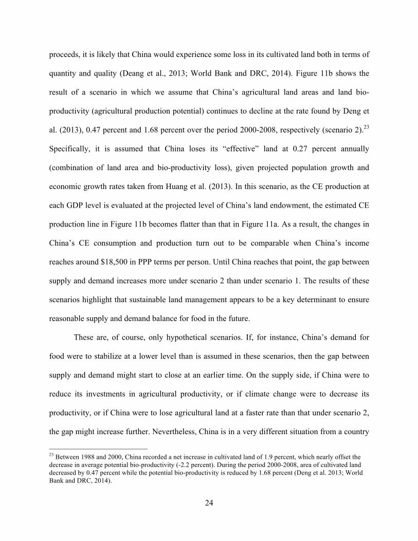
quantity and quality (Deang et al., 2013; World Bank and DRC, 2014). Figure 11b shows the

result of a scenario in which we assume that China’s agricultural land areas and land bio-

productivity (agricultural production potential) continues to decline at the rate found by Deng et

al. (2013), 0.47 percent and 1.68 percent over the period 2000-2008, respectively (scenario 2).23

Specifically, it is assumed that China loses its “effective” land at 0.27 percent annually

(combination of land area and bio-productivity loss), given projected population growth and

economic growth rates taken from Huang et al. (2013). In this scenario, as the CE production at

each GDP level is evaluated at the projected level of China’s land endowment, the estimated CE

production line in Figure 11b becomes flatter than that in Figure 11a. As a result, the changes in

China’s CE consumption and production turn out to be comparable when China’s income

reaches around $18,500 in PPP terms per person. Until China reaches that point, the gap between

supply and demand increases more under scenario 2 than under scenario 1. The results of these

scenarios highlight that sustainable land management appears to be a key determinant to ensure

reasonable supply and demand balance for food in the future.

These are, of course, only hypothetical scenarios. If, for instance, China’s demand for

food were to stabilize at a lower level than is assumed in these scenarios, then the gap between

supply and demand might start to close at an earlier time. On the supply side, if China were to

reduce its investments in agricultural productivity, or if climate change were to decrease its

productivity, or if China were to lose agricultural land at a faster rate than that under scenario 2,

the gap might increase further. Nevertheless, China is in a very different situation from a country

23 Between 1988 and 2000, China recorded a net increase in cultivated land of 1.9 percent, which nearly offset the decrease in average potential bio-productivity (-2.2 percent). During the period 2000-2008, area of cultivated land decreased by 0.47 percent while the potential bio-productivity is reduced by 1.68 percent (Deng et al. 2013; World Bank and DRC, 2014).

25

such as Japan or the Republic of Korea, where the much smaller land endowments almost ensure

that continuing large net imports of food will be required.

One important caveat of this study is that the data used for the analyses rely on

FAOSTAT data which in turn are based on official statistics. In particular, several scholars point

out that the livestock data for China are flawed (Fuller, Hayes and Smith, 2000; Ma, Huang and

Rozelle, 2004). Although we are aware of this potential bias in FAOSTAT data, it turns out to be

impossible for us to replace FAOSTAT data with revised data due to the lack of comparable data

for other countries. We therefore deal with this issue by conducting a sensitivity analysis in the

Appendix.

Some Policy Challenges

China’s ongoing shift in demand into more affluent, and particularly animal-based, foods is

likely to impose substantial pressure on agricultural resources and environment. In particular,

animal production puts pressure on land both directly 24 and indirectly through feedstuff

production. Cropland area tends to decrease as it competes for space with urban and industrial

uses. Since income growth is associated with both dietary upgrading and economic activities

which generate income, economic development is likely to intensify the competition for land. In

addition, the quality of China’s cultivated land is reportedly deteriorating due to soil degradation,

pollution and desertification (Chen, 2007; OECD and FAO, 2012; Ye and Ranst, 2009). Climate

change adds another challenge, as the overall impact of climate change on agricultural

productivity is likely to be negative (Ju, van der Velde, Lin, Xiong and Li, 2013).

Given increasingly tight resource constraints, the evolution of China’s net import demand

for food depends heavily on its productivity growth in agriculture. This is especially so, as China

24 About 20 percent of the world’s pastures and rangelands are degraded to some extent mainly through overgrazing. In China, the shift of production towards a large-scale grain-based industrial system appears to be leading to nutrient overload of soils and water pollution in some geographically concentrated areas (Steinfeld et al., 2006).  

26

continues to develop from an upper-middle to high income country.25 The experiences of high

income countries reveal that their agricultural output growth tends to rely increasingly on TFP

growth rather than input growth (Fuglie, 2012).26 The increase in productivity would also

generally have the desirable effect of increasing the incomes of farmers. In particular, it has very

powerful poverty-reducing impacts because so many of the poor—especially in China—live in

rural areas and depend on agriculture for their livelihoods (Christiaensen, Demery and

Kuhl,2011; Christiaensen, 2012).

Continued investment in R&D is likely to be a key factor for sustained growth of

agricultural output in China. However, as China’s land productivity has already attained a high

level, there is a possibility that further intensification of the use of cropland would result in

diminishing returns and environmental degradation (Brown, 1994; Wirsenius, 2010).

Technological developments beyond the focus on yield growth, in particular, to explore

sustainable management of natural resources and to address environmental concerns, seem likely

to become increasingly important. In contrast to China’s high land productivity, the labor

productivity of farmers in China remains low given China’s development level and relative to

other sectors of its economy. The shift of labor out of agriculture is likely to continue, imposing

challenges on China’s current labor-intensive, family based agricultural production system.

Some scholars point out that farm size in China is too small to reap economies of scale

necessary for domestic production to satisfy domestic demand (Otsuka, 2013). As China’s

comparative advantage has been shifting from the farm to the non-farm sector and the

25 According to the World Bank’s income classification, China moved up from “low” to “lower middle income” status in 1996 and further advanced to “upper middle income” status in 2010 (http://data.worldbank.org/about/country-classifications). 26 Decomposing agricultural output growth into contributions from inputs and TFP for the period 1960-2009, Fuglie (2012) shows that developed countries as a whole have relied increasingly on TFP growth to keep output from falling. Total agricultural inputs for developed countries as a group have been declining since the 1980s (Fuglie, 2012, Table 16.4).

27

opportunity cost of farm labor is rising, farm sizes need to be expanded, because the substitution

of large machines for labor requires scale economies (Otsuka, 2013; Yamauchi, 2014).

Promoting scale economies and mechanization is likely to involve a number of changes,

including development of land rental markets (Deininger and Jin, 2005; Zhang, Qingguo and Xu,

2004), institutional development such as machine rentals (Takahashi and Otsuka, 2009) as well

as removal of restrictions on labor movement from farm to non-farm sectors (Fan et al., 2003).

About one-third of the world’s farmers are still in China (Christiaensen, 2012). How to promote

farm size expansion while ensuring the well-being of smallholders is an important challenge

which requires future research. For instance, using farm panel data from Indonesia, Yamauchi

(2014) finds that while relatively large farmers tended to increase the scale of operation by

substituting machines for labor and by renting more land, such a dynamic change was not

observed among relatively small holders.

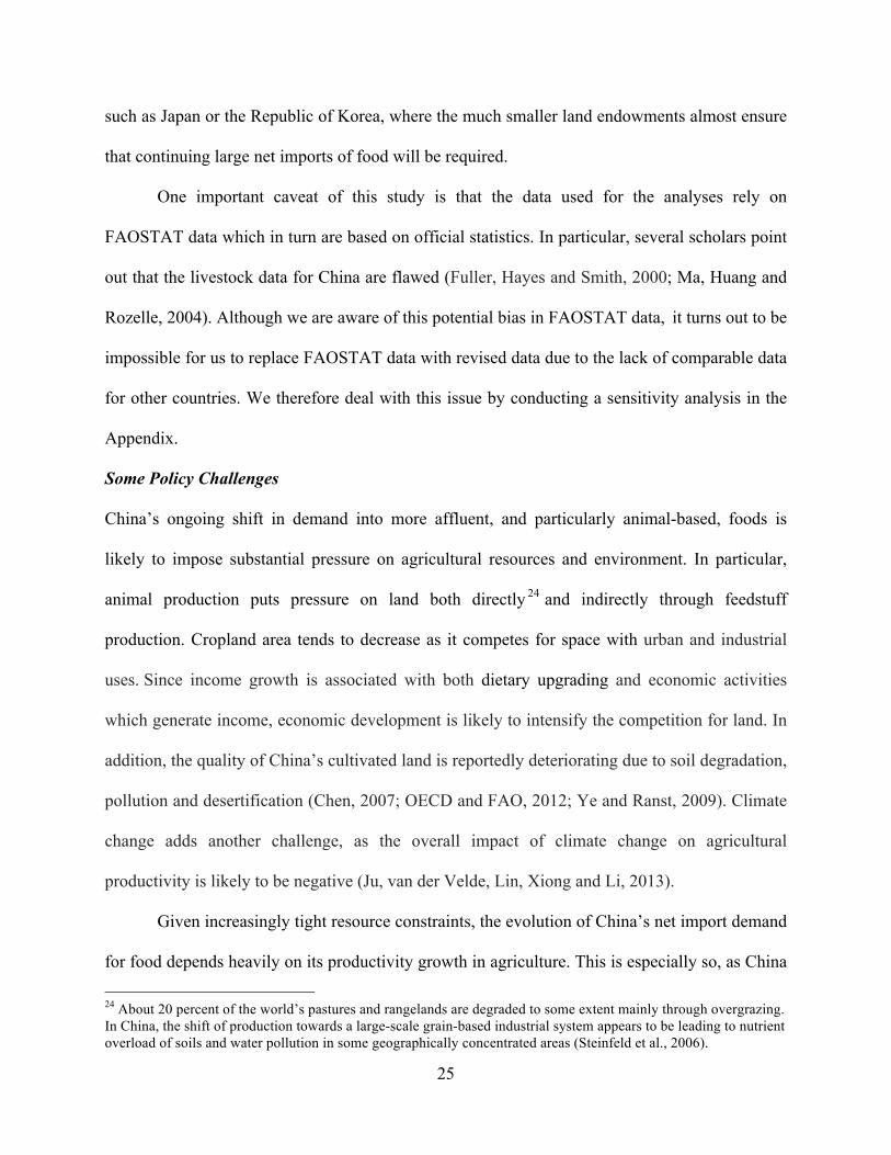
In principle, a gap between the demand and the supply for food could be diminished by a

protection policy that raises the price of all agricultural products relative to non-agricultural

products. However, this would have the undesirable effect of reducing the access of some poor

people to the staple foods that they need. In any event, as shown in Figures 12a and 12b, it

appears that per capita demand for key food staples, such as rice and wheat, is now declining

quite sharply in both urban and rural settings. This suggests that it is unlikely that the gap

between food demand and supply in China will manifest itself as large net imports of these

staples. Given this, there does not seem to be a self-sufficiency argument for increased protection

of these staple foods.

Protection for the feedstuffs demanded by China’s rapidly growing livestock production

sectors could reduce demand for these products, but would do so at the risk of hindering the

28

development of a modern livestock sector. Given China’s land constraints, such a policy, if

pursued strongly, could create a demand for imports of staple products by taking land out of

staple crops and potentially creating self-sufficiency concerns despite declining consumption of

these products.

4.  Conclusions  

This paper explored the evolution of China’s demand and supply for food using resource based

cereal equivalent measures of the type proposed by Yotopoulos (1985) and extended by Rask

and Rask (2004, 2011). We note that, while demand for food calories has probably come close to

its peak level in China, the ongoing shift in demand into high-protein, and particularly animal

based, foods induced by income growth, is likely to require a considerably greater agricultural

effort than would continuation of past demand patterns. Using the experience of a wide range of

countries, we find that China’s demand pattern—and the growth of that demand in terms of

cereal equivalents—is broadly similar to the international average.

On the supply side, we find that output of agricultural products in terms of their cereal

equivalents depends strongly on both the growth of income and on the country’s endowment of

agricultural land. Countries with much larger land endowments per person than China—that is

countries such as Brazil and the United States - tend to be exporters over a wide range of income

levels. By contrast, economies with much more limited land endowments than China’s –

economies such as Japan and the Republic of Korea—tend to become net food importers at a

relatively low income level and to remain net importers. China is a relatively land scarce country

with a per capita land endowment measured at about one-half of the world average. It appears

that China—probably because of the high productivity of much of its agricultural land and its

29

heavy investments in agricultural research and development—has produced much more food

than would be expected given its income level and land endowment.

The analyses of income-consumption-production dynamics suggest that China’s current

income level appears to fall in the range where consumption growth outstrips production growth,

widening its supply and demand gap for food. If China’s past outperformance can be maintained,

then it seems likely that, although China’s net imports of food will rise from current levels for a

while, the gap will begin to decline as China’s population growth and dietary transition slow

down. In the meantime, the quantity of agricultural resources that will be needed to feed the

Chinese population is likely to continue to increase. In particular, our simulation exercises show

that the evolution of the supply and demand gap for food depends on the changes in China’s

agricultural land availability both in terms of quantity and quality.

As China progresses from an upper-middle to a high income country, some loss of

agricultural land is likely and a large shift of labor out of agriculture is inevitable. The

experiences of developed countries reveal that they increasingly rely on agricultural productivity

growth in sustaining their agricultural output while their input growth rates tend to decline

(Fuglie, 2007; 2012). In conclusion, we suggest that continued agricultural productivity growth

through further investment in R&D, and through expansion in farm size and increased

mechanization, as well as sustainable management of agricultural resources, appear to be critical

for raising farm incomes and increasing food supplies to ensure that it is primarily China that

will feed China in the 21st century.    

30

References    

Alexandratos, N. and Bruinsma, J. World Agriculture towards 2030/2050: the 2012 Revision (No. 12-03). Agricultural Development Economics (ESA) Working Paper, (FAO, Rome, 2012).

Anderson, K. ‘Lobbying incentives and the pattern of protection in rich and poor Countries’,

Economic Development and Cultural Change, Vol. 43(2), (1995) pp. 401-23. Anderson, K. and Strutt A. ‘Food security policy options for China: lessons from other

countries’, Mimeo, (University of Adelaide, Australia, 2013). Atkin, D. ‘Trade, tastes and nutrition in India’, American Economic Review, Vol. 103(5), (2013)

pp. 1629-63. Brown, L. R. Who Will Feed China?: Wake-up Call for a Small Planet. (New York and London:

W.W. Norton & Company, 1995). Chen, J. ‘Rapid urbanization in China: a real challenge to soil protection and food security’,

Catena, Vol. 69(1), (2007) pp. 1-15. Christiaensen, L. The Role of Agriculture in a Modernizing Society: Food, Farms and Fields in

China 2030, (World Bank, Washington DC, 2012). Chapagain, A. K., Hoekstra, A. Y. and Savenije, H. H. G. ‘Water saving through international

trade of agricultural products,’ Hydrology and Earth System Sciences, Vol. 10(3), (2006) pp. 455-468.

Christiaensen, L., Demery, L. and Kuhl, J. ‘The role of agriculture in poverty reduction: an

empirical perspective’, Journal of Development Economics, Vol. 96, (2011) pp. 239–54. Clark, G., Huberman, M. and Lindert, P. ‘A British food puzzle, 1770-1850’, Economic History

Review’, Vol. 48(2), (1995) pp. 215-37. Deininger, K. and Jin, S. ‘The potential of land rental markets in the process of economic

development: evidence from China’, Journal of Development Economics, Vol. 78(1), (2005) pp. 241-270.

Deng, X., Huang, J. and Rozelle, S. ‘Impact of urbanization on land productivity and cultivated

land area in China’, Mimeo, (China Center for Agricultural Policy, Beijing, 2013). Elferink, E. V. and Nonhebel, S. ‘Variations in land requirements for meat production’, Journal

of Cleaner Production, Vol. 15(18), (2007) pp. 1778-1786. Fan, S., Zhang, X. and Robinson, S. ‘Structural change and economic growth in China’, Review

of Development Economics, Vol. 7(3), (2003) pp. 360-377.

31

Food and Agricultural Organization of the United Nations (FAO). Food Balance Sheet – A

Handbook. (FAO, Rome, 2001). Fiala, N. ‘Meeting the demand: an estimation of potential future greenhouse gas emissions from

meat production’, Ecological Economics, Vol. 67(3), (2008) pp. 412-419. Fuglie, K. ‘Productivity growth and technology capital in the global agricultural economy’, in K.

Fuglie, V. E. Ball and Wang, S. L. (eds.), Productivity Growth in Agriculture: An International Perspective, (CABI, UK, 2012) pp. 355-368.

Fuglie, K., MacDonald, J. M. and Ball, V. E. ‘Productivity growth in US agriculture’, USDA-

ERS Economic Brief, Vol. 9. (2007). Fuller, F., Hayes, D. and Smith, D. ‘Reconciling Chinese meat production and consumption

data’, Economic Development and Cultural Change, Vol. 49(1), (2000) pp. 23-43.

Garnett, T. ‘Livestock-related greenhouse gas emissions: Impacts and options for policy makers’, Environmental Science and Policy’, Vol. 12(4), (2009) pp. 491-503.

Gerbens-Leenes, P. W. and Nonhebel, S. ‘Consumption patterns and their effects on land

required for food’, Ecological Economics, Vol. 42(1), (2002a) pp. 185-199. Gerbens-Leenes, P. W., Nonhebel, S., and Ivens, W. P. M. F. ‘A method to determine land

requirements relating to food consumption patterns’, Agriculture, Ecosystems & Environment, Vol. 90(1), (2002b) pp. 47-58.

Gerber, P. J., Steinfeld, H., Henderson, B., Mottet, A., Opio, C., Dijkman, J., Falcucci, A. and

Tempio, G. Tackling Climate Change through Livestock: a Global Assessment of Emissions and Mitigation Opportunities. (FAO, Rome, 2013).

Hoekstra, A. Y. and Hung, P. Q. ‘Globalization of water resources: International virtual water

flows in relation to crop trade’, Global Environmental Change, Vol. 15(1), (2005) pp. 45-56.

Huang, J. and David, C. ‘Demand for cereal grains in Asia: the effect of urbanization’,

Agricultural Economics, Vol. 8, (1993), pp. 107-24. Huang, J. and Rozelle, S. ‘Technological change: Rediscovering the engine of productivity

growth in China's rural economy’, Journal of Development Economics, Vol. 49(2), (1996) pp. 337-369.

Huang, J., Rozelle, S. and Yang, J. ‘Urbanization and China’s food security’, Mimeo, (China

Center for Agricultural Policy, Beijing, 2013).

32

International Food Policy Research Institute (IFPRI)). ASTI Global Assessment of Agricultural R&D Spending, (IFPRI, Washington DC., 2012).

Jia, L. and Petrick, M. ‘How does land fragmentation affect off-­‐farm labor supply: Panel data

evidence from China’, Agricultural Economics, Vol. 45, (2013) pp. 1-12. Jin, S., Huang, J., Hu, R. and Rozelle, S. ‘The creation and spread of technology and total factor

productivity in China's agriculture’, American Journal of Agricultural Economics, Vol. 84(4), (2002). pp. 916-930.

Ju, H., van der Velde, M., Lin, E., Xiong, W. and Li, Y. ‘The impacts of climate change on

agricultural production systems in China’, Climatic Change, Vol. 120(1-2), (2013) pp. 313-324.

Kearney, J. ‘Food consumption trends and drivers’, Philosophical Transactions of the Royal

Society B: Biological Sciences, Vol. 365(1554), (2010) pp. 2793-2807. Kuijs, L. and Wang, T. ‘China's pattern of growth: Moving to sustainability and reducing

inequality,’ China and World Economy, Vol. 14(1), (2006) pp. 1-14. Li, G., Zhao, Y., and Cui, S. ‘Effects of urbanization on arable land requirements in China, based

on food consumption patterns’, Food Security, Vol. 5(3), (2013) pp. 439-449. Ma, H., Huang, J. and Rozelle, S. ‘Reassessing China’s livestock statistics: An analysis of

discrepancies and the creation of new data series’, Economic Development and Cultural Change, Vol. 52(2), (2004) pp. 445-73, January.

Martin, W. and Mitra, D. ‘Productivity growth and convergence in agriculture and

manufacturing’, Economic Development and Cultural Change’, Vol. 49(2), (2001) pp. 403-23, January.

Martin, W. and Porter, D. ‘Testing for changes in the structure of demand for meat in Australia’,

Australian Journal of Agricultural Economics, Vol. 29(1), (1985) pp. 16-31. Martin, W. and Warr, P. ‘Explaining agriculture's relative decline: a supply side analysis for

Indonesia’, World Bank Economic Review, Vol. 7(3), (1993) pp. 381-401, September. Nin-Pratt, A., Yu, B., and Fan, S. ‘Comparisons of agricultural productivity growth in China and

India’, Journal of Productivity Analysis, Vol. 33(3), (2010) pp. 209-223. OECD and FAO. ‘Feeding China: Prospects and challenges in the next decade’, Chapter 2 in

OECD-FAO Agricultural Outlook 2013-2022, (Paris: OECD Publishing, 2013). Otsuka, K. ‘Food insecurity, income inequality, and the changing comparative advantage in

world agriculture’, Agricultural Economics, Vol. 44(s1), (2013) pp. 7-18.

33

Qiang, W., Liu, A., Cheng, S., Kastner, T. and Xie, G. ‘Agricultural trade and virtual land use: The case of China's crop trade’, Land Use Policy, Vol. 33, (2013) pp. 141-150.

Rask, K. and Rask, N. ‘Economic development and food production–consumption balance: A

growing global challenge’, Food Policy, Vol. 36(2), (2011) pp. 186-96. Rask, K. and Rask, N. ‘Reaching turning points in economic transition: Adjustments to

distortions in resource-based consumption of food’, Comparative Economic Studies, Vol. 46(4), (2004) pp. 542-569.

Robinson, T., Thornton, P., Franceschini, G., Kruska, R., Chiozza, F., Notenbaert, A. and You, L.

Global Livestock Production Systems. (FAO, Rome, 2011). Rozelle, S. and Swinnen, J. F. ‘Success and failure of reform: Insights from the transition of

agriculture’, Journal of Economic Literature, Vol. 42(2), (2004) pp. 404-456. Satterthwaite, D., McGranahan, G. and Tacoli, C. ‘Urbanization and its implications for food and

farming’, Philosophical Transactions of the Royal Society, Vol. B 365, (2010) pp. 2809–20.

Steinfeld, H., Gerber, P., Wassenaar, T., Castel, V., Rosales, M. and De Haan, C. Livestock's

Long Shadow. (FAO, Rome, 2006). Takahashi, K. and Otsuka, K. ‘The increasing importance of nonfarm income and the changing

use of labor and capital in rice farming: the case of Central Luzon, 1979–2003’, Agricultural Economics, Vol. 40(2), (2009) pp. 231-242.

United States Department of Agriculture (USDA). Livestock-Feed Relationships, National and

State. (USDA, Washington, DC, 1975). Wang, J., Huang, J. and Rozelle, S. ‘Water and urbanization in China’, Mimeo, (China Center

for Agricultural Policy, Beijing, 2013). Weiming, T. and Ying, G. ‘The effects of trade liberalization on the development of China’s

soybean sector’, Regional Trade Agreements and Food Security in Asia, 339. (2012). Wirsenius, S. ‘Efficiencies and biomass appropriation of good commodities on global and

regional levels’, Agricultural Systems, Vol. 77(3), (2003) pp. 219-255. Wirsenius, S., Azar, C. and Berndes, G. ‘How much land is needed for global food production

under scenarios of dietary changes and livestock productivity increases in 2030?’ Agricultural Systems, Vol. 103(9), (2010) pp. 621-638.

Williams, A., Audsley, E. and Sandars, D. Determining the Environmental Burdens and

Resource Use in the Production of Agricultural and horticultural commodities: Defra Project Report IS0205. (Bedford: Cranfiled University and Defra, 2006).

34

World Bank and the Development Research Centre (DRC) of State Council, China’s

Urbanization and Food Security, (World Bank and DRC, Washington DC and Beijing, 2014).

Yamauchi, F. ‘Wage growth, landholding and mechanization in agriculture: Evidence form

Indonesia’, Policy Research Working Paper, #6789, (World Bank, Washington, DC, 2014).

Ye, L. and Van Ranst, E. ‘Production scenarios and the effect of soil degradation on long-term

food security in China’, Global Environmental Change, Vol. 19(4), (2009) pp. 464-481. Yotopoulos, P. A. ‘Middle-income classes and food crises: The "new" food-feed competition’,

Economic Development and Cultural Change, Vol. 33(3), (1985) pp. 463-483. Zhang, Q. F., Qingguo, M. and Xu, X. ‘Development of land rental markets in rural Zhejiang:

growth of off-farm jobs and institution building,’ The China Quarterly, Vol. 180, (2004) pp. 1031-1049.

Zhen, L., Cao, S., Cheng, S., Xie, G., Wei, Y., Liu, X. and Li, F. ‘Arable land requirements

based on food consumption patterns: Case study in rural Guyuan District, western China’, Ecological Economics, Vol. 69(7), (2010) pp. 1443-1453.

Figure 1a C

alorie Intake per capita by Selected Countries for the period 1980-2009

Source: FAO

STAT

0  

500  

1000  

1500  

2000  

2500  

3000  

3500  

4000  

1980  

1983  

1986  

1989  

1992  

1995  

1998  

2001  

2004  

2007  

Total  Calories  (kcal/capita/day)  

0  

500  

1000  

1500  

2000  

2500  

3000  

3500  

4000  

1980  

1983  

1986  

1989  

1992  

1995  

1998  

2001  

2004  

2007  

Crops  Calories  (kcal/capita/day)  

0  

500  

1000  

1500  

2000  

2500  

3000  

3500  

4000  

1980  

1983  

1986  

1989  

1992  

1995  

1998  

2001  

2004  

2007  

Livestock/fish  Calories  (kcal/capita/day)  

China  

EU  

Japan  

Korea  

USA  

World  

36

Figure 1b Protein Intake per capita by Selected Countries for the period 1980-2009

Source: FAO

STAT

0  

20  

40  

60  

80  

100  

120  

Total  Protein  (g/capita/day)  

0  

20  

40  

60  

80  

100  

120  

1980  

1983  

1986  

1989  

1992  

1995  

1998  

2001  

2004  

2007  

Crops  Protein  (g/capita/day)  

0  

20  

40  

60  

80  

100  

120  

1980  

1983  

1986  

1989  

1992  

1995  

1998  

2001  

2004  

2007  

Livestock/fish  Protein  (g/capita/day)  China  

EU  

Japan  

Korea  

USA  

World  

37

Figure 1c Fat Intake per capita by Selected Countries for the period 1980-2009

Source: FAO

STAT

0  

20  

40  

60  

80  

100  

120  

140  

160  

180  

1980  1982  1984  1986  1988  1990  1992  1994  1996  1998  2000  2002  2004  2006  2008  

Total  Fat  (g/capita/day)  

0  

20  

40  

60  

80  

100  

120  

140  

160  

180  

1980  1982  1984  1986  1988  1990  1992  1994  1996  1998  2000  2002  2004  2006  2008  

Fat  from  Crops(g/capita/day)  

0  

20  

40  

60  

80  

100  

120  

140  

160  

180  

1980  1983  1986  1989  1992  1995  1998  2001  2004  2007  

Livestock/fish  Fat  (g/capita/day)  China  

EU  

Japan  

Korea  

USA  

World  

38

Figure 2a Self Sufficiency Ratios for Grains in Asian Countries (%)

Source: Production, Supply and Distribution (PSD) data, USDA. Notes: Total for rice, wheat, maize and soybeans. Self-sufficiency is measured by dividing (gross) production by (gross) domestic consumption excluding stock changes. Gross production and consumption include uses for non-food purposes such as feed use. Figure 2b Contribution of Supply-Demand Gap by Major Grains for China (1000 tons)

Source: Production, Supply and Distribution (PSD) data, USDA. Notes: The figures reflect the differences between production and consumption, which are the sum of net imports and the changes in stock (Production – Consumption = Exports – Imports + Changes in stock).

0  

20  

40  

60  

80  

100  

120  

140  

160  

180  

200  

1960/1961  

1963/1964  

1966/1967  

1969/1970  

1972/1973  

1975/1976  

1978/1979  

1981/1982  

1984/1985  

1987/1988  

1990/1991  

1993/1994  

1996/1997  

1999/2000  

2002/2003  

2005/2006  

2008/2009  

2011/2012  

China  

Japan  

Korea  

Taiwan  

Indonesia  

Philippines  

Thailand  

Bangladesh  

India  

-­‐80000  

-­‐70000  

-­‐60000  

-­‐50000  

-­‐40000  

-­‐30000  

-­‐20000  

-­‐10000  

0  

10000  

20000  

30000  

1960/1961  

1963/1964  

1966/1967  

1969/1970  

1972/1973  

1975/1976  

1978/1979  

1981/1982  

1984/1985  

1987/1988  

1990/1991  

1993/1994  

1996/1997  

1999/2000  

2002/2003  

2005/2006  

2008/2009  

2011/2012  

Corn  

Soybean  

Rice  

Wheat  

39

Figure 3a Evolution of CE Consumption in China:

Crops vs. Animal Products (million tons)

Source: Authors’ calculation

Figure 3b Population in China 1980-2030 (million)

Source: FAOSTAT Note: The series consist of both estimates and projections.

Figure 3c Decomposition of Change in CE Consumption: Population Growth vs. Diet Changes (million tons)

Source: Authors’ calculation

0  

200  

400  

600  

800  

1000  

1200  

1400  

1600  

1980  1982  1984  1986  1988  1990  1992  1994  1996  1998  2000  2002  2004  2006  2008  

Crops   Animal  products  

800  

900  

1000  

1100  

1200  

1300  

1400  

1500  

1980  

1982  

1984  

1986  

1988  

1990  

1992  

1994  

1996  

1998  

2000  

2002  

2004  

2006  

2008  

2010  

2012  

2014  

2016  

2018  

2020  

2022  

2024  

2026  

2028  

2030  

0  

200  

400  

600  

800  

1000  

1200  

1400  

1600  

1980  1982  1984  1986  1988  1990  1992  1994  1996  1998  2000  2002  2004  2006  2008  

1980  level   Diet  Changes     PopulaNon  Changes  

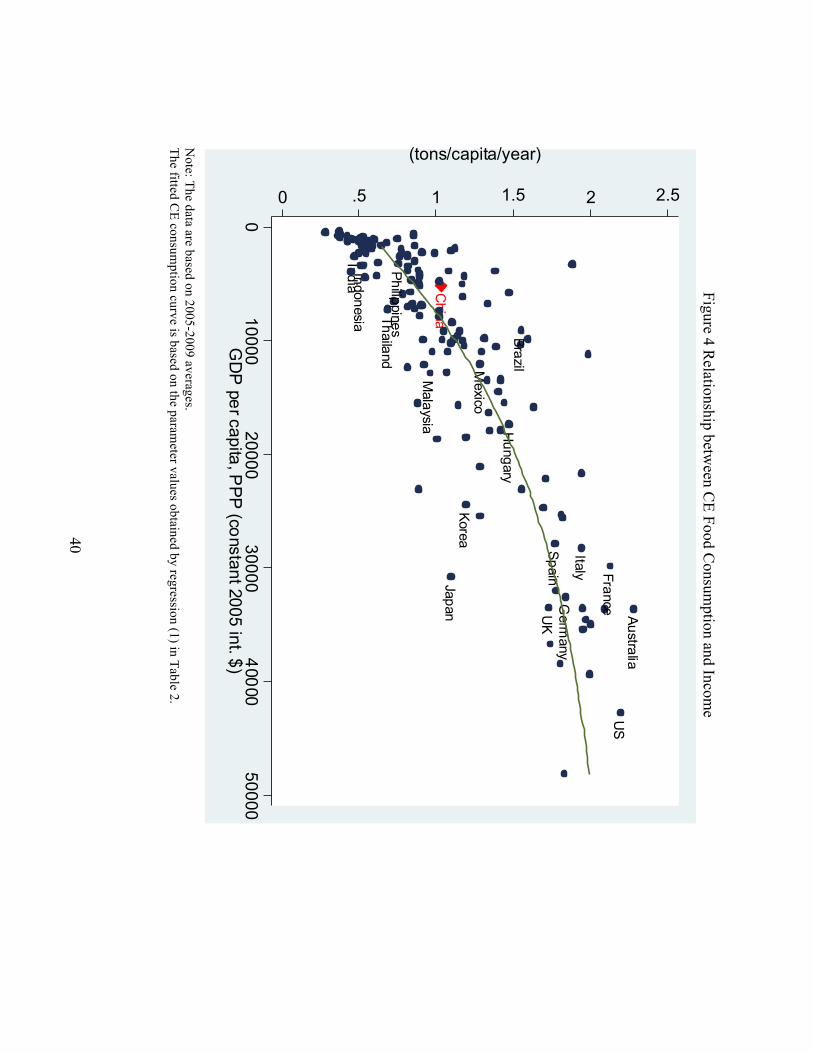
40

Figure 4 Relationship betw

een CE Food C

onsumption and Incom

e

N

ote: The data are based on 2005-2009 averages. The fitted C

E consumption curve is based on the param

eter values obtained by regression (1) in Table 2.

China

India

Germ

any

Malaysia

Japan

Indonesia

Italy

Hungary

US

Korea

Australia

Mexico

UK

Spain

Brazil

ThailandPhilippines

France0 .5 1 1.5 2 2.5

(tons/capita/year)

010000

2000030000

4000050000

GD

P per capita, P

PP (constant 2005 int. $)

41

Figure 5 Grow

th Trend of CE Food C

onsumption 1980-2009

` N

otes: The starting and ending points of the arrows represent the C

E consumptions for the year 1980 and 2009 respectively.

The fitted CE consum

ption curve is based on the parameter values obtained by regression (2) in Table 2.

AustraliaAustraliaAustraliaAustraliaAustraliaAustraliaAustraliaAustraliaAustraliaAustraliaAustraliaAustraliaAustraliaAustraliaAustraliaAustraliaAustraliaAustraliaAustraliaAustraliaAustraliaAustraliaAustraliaAustraliaAustraliaAustraliaAustraliaAustraliaAustraliaAustralia

BrazilBrazilBrazilBrazilBrazilBrazilBrazilBrazilBrazilBrazilBrazilBrazilBrazilBrazilBrazilBrazilBrazilBrazilBrazilBrazilBrazilBrazilBrazilBrazilBrazilBrazilBrazilBrazilBrazilBrazil

China

China

China

China

China

China

China

China

China

China

China

China

China

China

China

China

China

China

China

China

China

China

China

China

China

China

China

China

China

China

FranceFranceFranceFranceFranceFranceFranceFranceFranceFranceFranceFranceFranceFranceFranceFranceFranceFranceFranceFranceFranceFranceFranceFranceFranceFranceFranceFranceFranceFranceG

ermany

Germ

anyG

ermany

Germ

anyG

ermany

Germ

anyG

ermany

Germ

anyG

ermany

Germ

anyG

ermany

Germ

anyG

ermany

Germ

anyG

ermany

Germ

anyG

ermany

Germ

anyG

ermany

Germ

anyG

ermany

Germ

anyG

ermany

Germ

anyG

ermany

Germ

anyG

ermany

Germ

anyG

ermany

Germ

any

Hungary

Hungary

Hungary

Hungary

Hungary

Hungary

Hungary

Hungary

Hungary

Hungary

Hungary

Hungary

Hungary

Hungary

Hungary

Hungary

Hungary

Hungary

Hungary

Hungary

Hungary

Hungary

Hungary

Hungary

Hungary

Hungary

Hungary

Hungary

Hungary

Hungary

IndiaIndiaIndiaIndiaIndiaIndiaIndiaIndiaIndiaIndiaIndiaIndiaIndiaIndiaIndiaIndiaIndiaIndiaIndiaIndiaIndiaIndiaIndiaIndiaIndiaIndiaIndiaIndiaIndiaIndia

IndonesiaIndonesiaIndonesiaIndonesiaIndonesiaIndonesiaIndonesiaIndonesiaIndonesiaIndonesiaIndonesiaIndonesiaIndonesiaIndonesiaIndonesiaIndonesiaIndonesiaIndonesiaIndonesiaIndonesiaIndonesiaIndonesiaIndonesiaIndonesiaIndonesiaIndonesiaIndonesiaIndonesiaIndonesiaIndonesia

ItalyItalyItalyItalyItalyItalyItalyItalyItalyItalyItalyItalyItalyItalyItalyItalyItalyItalyItalyItalyItalyItalyItalyItalyItalyItalyItalyItalyItalyItaly

JapanJapanJapanJapanJapanJapanJapanJapanJapanJapanJapanJapanJapanJapanJapanJapanJapanJapanJapanJapanJapanJapanJapanJapanJapanJapanJapanJapanJapanJapan

KoreaKoreaKoreaKoreaKoreaKoreaKoreaKoreaKoreaKoreaKoreaKoreaKoreaKoreaKoreaKoreaKoreaKoreaKoreaKoreaKoreaKoreaKoreaKoreaKoreaKoreaKoreaKoreaKoreaKorea

Malaysia

Malaysia

Malaysia

Malaysia

Malaysia

Malaysia

Malaysia

Malaysia

Malaysia

Malaysia

Malaysia

Malaysia

Malaysia

Malaysia

Malaysia

Malaysia

Malaysia

Malaysia

Malaysia

Malaysia

Malaysia

Malaysia

Malaysia

Malaysia

Malaysia

Malaysia

Malaysia

Malaysia

Malaysia

Malaysia

Mexico

Mexico

Mexico

Mexico

Mexico

Mexico

Mexico

Mexico

Mexico

Mexico

Mexico

Mexico

Mexico

Mexico

Mexico

Mexico

Mexico

Mexico

Mexico

Mexico

Mexico

Mexico

Mexico

Mexico

Mexico

Mexico

Mexico

Mexico

Mexico

Mexico

Philippines

Philippines

Philippines

Philippines

Philippines

Philippines

Philippines

Philippines

Philippines

Philippines

Philippines

Philippines

Philippines

Philippines

Philippines

Philippines

Philippines

Philippines

Philippines

Philippines

Philippines

Philippines

Philippines

Philippines

Philippines

Philippines

Philippines

Philippines

Philippines

Philippines

SpainSpainSpainSpainSpainSpainSpainSpainSpainSpainSpainSpainSpainSpainSpainSpainSpainSpainSpainSpainSpainSpainSpainSpainSpainSpainSpainSpainSpainSpain

ThailandThailandThailandThailandThailandThailandThailandThailandThailandThailandThailandThailandThailandThailandThailandThailandThailandThailandThailandThailandThailandThailandThailandThailandThailandThailandThailandThailandThailandThailand

UK

UK

UK

UK

UK

UK

UK

UK

UK

UK

UK

UK

UK

UK

UK

UK

UK

UK

UK

UK

UK

UK

UK

UK

UK

UK

UK

UK

UK

UK

US

US

US

US

US

US

US

US

US

US

US

US

US

US

US

US

US

US

US

US

US

US

US

US

US

US

US

US

US

US

0 .5 1 1.5 2 2.5

(tons/capita/year)

010000

2000030000

4000050000

GD

P per capita, P

PP (constant 2005 int. $)

42

Figure 6 Calorie vs. C

E Consom

ption 1980-2009

N

otes: The fitted CE consum

ption curve (right-hand side) is based on the parameter values obtained by regression (2) in Table 2. The fitted

calorie consumption line (left-hand side) is based on the param

eter values obtained using the same functional form

as the CE consum

ption estim

ate (equation (1)). During the period 2005-2009, the w

orld average per capita cereal consumption w

as 0.403 kilogram per day (.147 ton per

year) which contained 1,296 kcal per day on average. Thus, one ton of C

E per capita per year is equivalent to about 8800 kcal per capita per day (1,296/.147≈8800).

0 .5 1 1.5 2(tons/capita/year)

0 5000 10000 15000

(kcal/capita/day)

010000

2000030000

4000050000

Real G

DP(P

PP) per capita in 2005 int. $ 1980-2009

China C

alorie Consum

ptionFitted C

alorie Consum

ption

China C

E Consum

ptionFitted C

E Consum

ption

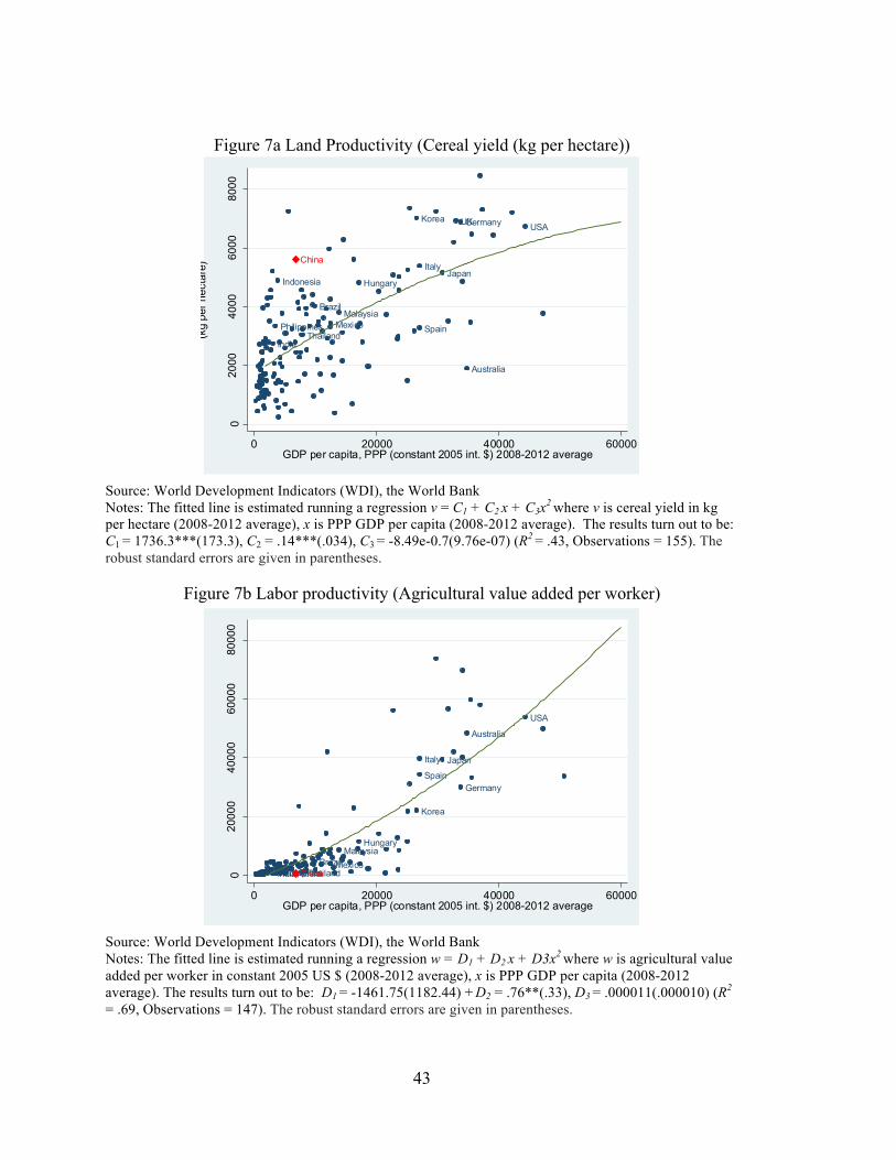
43

Figure 7a Land Productivity (Cereal yield (kg per hectare))

Source: World Development Indicators (WDI), the World Bank Notes: The fitted line is estimated running a regression v = C1 + C2 x + C3x2 where v is cereal yield in kg per hectare (2008-2012 average), x is PPP GDP per capita (2008-2012 average). The results turn out to be: C1 = 1736.3***(173.3), C2 = .14***(.034), C3 = -8.49e-0.7(9.76e-07) (R2 = .43, Observations = 155). The robust standard errors are given in parentheses.

Figure 7b Labor productivity (Agricultural value added per worker)

Source: World Development Indicators (WDI), the World Bank Notes: The fitted line is estimated running a regression w = D1 + D2 x + D3x2 where w is agricultural value added per worker in constant 2005 US $ (2008-2012 average), x is PPP GDP per capita (2008-2012 average). The results turn out to be: D1 = -1461.75(1182.44) + D2 = .76**(.33), D3 = .000011(.000010) (R2

= .69, Observations = 147). The robust standard errors are given in parentheses.

Australia

Brazil

Germany

Hungary

India

Indonesia

ItalyJapan

Korea

MalaysiaMexicoPhilippines Spain

Thailand

UK USA

China

020

0040

0060

0080

00

(kg

per h

ecta

re)

0 20000 40000 60000GDP per capita, PPP (constant 2005 int. $) 2008-2012 average

Australia

Brazil

Germany

Hungary

IndiaIndonesia

Italy Japan

Korea

MalaysiaMexico

Philippines

Spain

Thailand

USA

China020

000

4000

060

000

8000

0

(Con

stan

t 200

5 U

S $

)

0 20000 40000 60000GDP per capita, PPP (constant 2005 int. $) 2008-2012 average

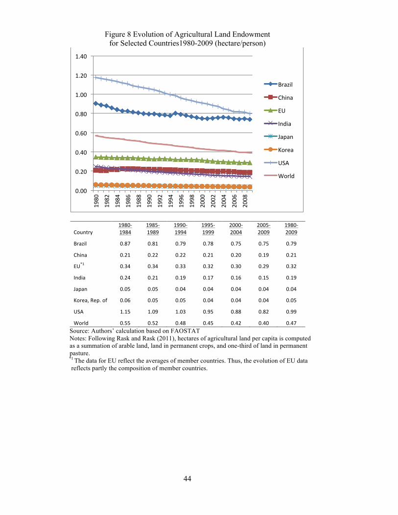
44

Figure 8 Evolution of Agricultural Land Endowment for Selected Countries1980-2009 (hectare/person)

Country  1980-­‐1984  

1985-­‐1989  

1990-­‐1994  

1995-­‐1999  

2000-­‐2004  

2005-­‐2009  

1980-­‐2009  

Brazil   0.87   0.81   0.79   0.78   0.75   0.75   0.79  

China   0.21   0.22   0.22   0.21   0.20   0.19   0.21  

EU*1   0.34   0.34   0.33   0.32   0.30   0.29   0.32  

India   0.24   0.21   0.19   0.17   0.16   0.15   0.19  

Japan   0.05   0.05   0.04   0.04   0.04   0.04   0.04  

Korea,  Rep.  of   0.06   0.05   0.05   0.04   0.04   0.04   0.05  

USA   1.15   1.09   1.03   0.95   0.88   0.82   0.99  

World   0.55   0.52   0.48   0.45   0.42   0.40   0.47   Source: Authors’ calculation based on FAOSTAT Notes: Following Rask and Rask (2011), hectares of agricultural land per capita is computed as a summation of arable land, land in permanent crops, and one-third of land in permanent pasture. *1 The data for EU reflect the averages of member countries. Thus, the evolution of EU data reflects partly the composition of member countries.

0.00  

0.20  

0.40  

0.60  

0.80  

1.00  

1.20  

1.40  

1980  

1982  

1984  

1986  

1988  

1990  

1992  

1994  

1996  

1998  

2000  

2002  

2004  

2006  

2008  

Brazil  

China  

EU  

India  

Japan  

Korea  

USA  

World  

45

Figure 9 Relationship betw

een CE Production and Incom

e at China’s Land Endow

ment Level

Note: The data are based on 2005-2009 averages.

India

Germ

anyM

alaysia

JapanIndonesia

Italy

China

Hungary

US

Korea

Australia

Mexico

UK

Spain

Brazil

ThailandPhilippines

France

0 1 2 3

(tons/capita/year)

010000

2000030000

4000050000

GD

P per capita, PPP 2005 int. $

China C

E Consum

ptionC

hina CE Production

CE Production adjusted at C

hina Land LevelC

E Production, land=.21 ha (China)

46

Figure 10a CE Consumption and CE Production for China and India 1980-2009

Figure 10b CE Consumption and CE Production 1980-2009 Examples for Relatively Land Abundant Countries: Brazil and the United States

.51

1.5

22.

5

(tons

/cap

ita/y

ear)

0 10000 20000 30000 40000 50000Real GDP(PPP) per capita in 2005 int. $ 1980-2009

China CE Consumption 1980-2009 China CE Production 1980-2009India CE Consumption 1980-2009 India CE Production 1980-2009

CE Production, land=.21 ha (China) CE Production, land=.19 ha (India)

CE Consumption

01

23

4

(tons

/cap

ita/y

ear)

0 10000 20000 30000 40000 50000Real GDP(PPP) per capita in 2005 int. $ 1980-2009

Brazil CE Consumption 1980-2009 Brazil CE Production 1980-2009US CE onsumption 1980-2009 US CE Production 1980-2009

CE Production, land=.79 ha (Brazil) CE Production, land=.99 ha (USA)

CE Consumption

47

Figure 10c CE Consumption and CE Production 1980-2009:

Examples for Relatively Land Scarce Countries: Japan and Republic of Korea

.51

1.5

2

(tons

/cap

ita/y

ear)

0 10000 20000 30000 40000 50000Real GDP(PPP) per capita in 2005 int. $ 1980-2009

Japan CE Consumption 1980-2009 Japan CE Production 1980-2009Korea CE Consumption 1980-2009 Korea CE Production 1980-2009

CE Production, land=.04 ha (Japan) CE Production, land=.05 ha (Korea)

CE Consumption

48

Figure 11a CE Production and CE Consumption Assuming China’s Residuals Reflect a Sustained Difference (Scenario 1)

Figure 11b CE Production and CE Consumption Assuning China’s Experiencing Loss of Land Area and Quality (Scenario 2)

.51

1.5

2

(tons

/cap

ita/y

ear)

0 10000 20000 30000GDP per capita, PPP 2005 int. $

China CE consumption1980-2009 China CE production 1980-2009

Shifted CE production line Shifted CE consumption line

.51

1.5

2

(tons

/cap

ita/y

ear)

0 10000 20000 30000GDP per capita, PPP 2005 int. $

China CE consumption1980-2009 China CE production 1980-2009

Shifted CE production line Shifted CE consumption line

49

Figure 12a. Average Annual Consumption of Food: Urban Residents, 1957-2011(kg)

Source: World Bank staff calculation based on DRC data Note: Data unavailable for milk and fruits before 1990; data for milk and fruits from 1996-1998 estimated based on averages of 1995 and 1999.

Figure 12b. Average Annual Consumption of Food: Rural Residents, 1978-2011 (kg)

-­‐  Source: World Bank staff calculation based on DRC data  Note: Protein foods include pork, beef, lamb, poultry, seafood, and egg. Data unavailable for dairy products before 1982, and for vegetables and dairy products in 2011.

0  

20  

40  

60  

80  

100  

120  

140  

160  

180  

1957  

1964  

1981  

1982  

1983  

1984  

1985  

1986  

1987  

1988  

1989  

1990  

1991  

1992  

1993  

1994  

1995  

1996  

1997  

1998  

1999  

2000  

2003  

2004  

2005  

2006  

2007  

2008  

2009  

2010  

2011  

Vegetables  

Grains  

Fruits  

Protein  Foods**    

Cooking  Oil  

Milk  

0  

50  

100  

150  

200  

250  

300  

1978  

1979  

1980  

1981  

1982  

1983  

1984  

1985  

1986  

1987  

1988  

1989  

1990  

1991  

1992  

1993  

1994  

1995  

1996  

1997  

1998  

1999  

2000  

2001  

2002  

2003  

2004  

2005  

2006  

2007  

2008  

2009  

2010  

2011  

Grains

Vegetables

Protein Foods**

Cooking Oil

Dairy Products

50

Appendix: Some Sensitivity Analysis: CE Production and CE Consumption Using Alternative Livestock Data

Several scholars have argued that the Food Balance Sheets (FBSs) data for China from FAOSTAT, which are based on official Chinese statistics, are biased. In particular, livestock production is widely believed to be over reported introducing potentially serious bias into food supply and demand balance estimates (e.g., Fuller, Hayes and Smith, 2000; Ma, Huang and Rozelle, 2004). Ma et al. (2004) provide revised series on production and consumption for livestock products for China over the period 1980 to 1999. Their results on livestock production are lower than the official numbers up to 1999, although they still show rapid growth with, for instance, a tripling of pork production over the 1980 to 1999 period, rather than an increase of three and a half times. To our knowledge, after 1999, revised livestock production and consumption data are available only for 2000, 2010 and 2012 from the China Agricultural Policy Simulation Model (CAPSiM) (Huang et al., 2013). To see how sensitive our results might be to the use of alternative data, we repeat scenario 1 (Figure 11a), replacing 2009 livestock data (which is the latest year available in FBSs) with the 2010 livestock production and consumption data from the CAPSiM model (Huang et al., 2013). The results suggest that China’s CE production point is close to the global trend, rather than substantially above the trend, while its consumption point turns out to be below the global trend.27 Following the assumptions in scenario 1, we shift both CE production and consumption curves so that they cross China’s alternative CE production and consumption points. The shifted lines suggest that China’s current income level lies in the range where consumption growth outpaces production growth, but that the gap will likely start to decrease as China’s consumption growth rate declines. However, evaluating the bias of FBSs data is not within the scope of this study and further studies are required to address the data quality issues.

Figure A CE Production and Consumption With Alternative Livestock data

27 Since the two datasets are not directly comparable, the difference in the results may be influenced by the differences in characteristics of the datasets. For instance, Kearney (2010) suggests that the FBSs data generally tend to overestimate consumption since they are referring to “available” rather than “actual” food consumption.

0.5

11.

52

(ton

s/ca

pita

/yea

r)

0 10000 20000 30000GDP per capita, PPP 2005 int. $

China CE consumption (alternative data) China CE production (al ternative data)

Shifted CE production Shifted CE consummption