Where am I? SLAM for Mobile Machineson A Smart Working Site

1st Yusheng Xiang, 7th Marcus GeimerInstitute of Vehicle System Technology

Karlsruhe Institute of TechnologyKarlsruhe, Germany

yusheng.xiang@partner.kit.edu

2nd Dianzhao LiInstitute of Vehicle System Technology

Karlsruhe Institute of TechnologyKarlsruhe, Germanydianzhao.li@kit.edu

3rd Tianqing SuGuanghua School of Management

Peking UniversityBeijing, China

tianqing.su@hotmail.com

4th Quan ZhouVehicle and Engine Research Centre

University of BirminghamBirmingham, UK

q.zhou@bham.ac.uk

5th Christine BrachDivision of Mobile Hydraulics

Robert Bosch GmbHElchingen, Germany

christine.brach@boschrexroth.de

6th Samuel S. MaoDepartment of Mechanical Engineering

University of California, BerkeleyBerkeley, USA

ssmao@berkeley.edu

Abstract—The current optimization approaches of construc-tion machinery are mainly based on internal sensors. However,the decision of a reasonable strategy is not only determined byits intrinsic signals, but also very strongly by environmentalinformation, especially the terrain. Due to the dynamicallychanging of the construction site and the consequent absence of ahigh definition map, the Simultaneous Localization and Mapping(SLAM) offering the terrain information for construction ma-chines is still challenging. Current SLAM technologies proposedfor mobile machines are strongly dependent on costly or com-putationally expensive sensors, such as RTK GPS and cameras,so that commercial use is rare. In this study, we proposed anaffordable SLAM method to create a multi-layer gird map for theconstruction site so that the machine can have the environmentalinformation and be optimized accordingly. Concretely, after themachine passes by, we can get the local information and recordit. Combining with positioning technology, we then create a mapof the interesting places of the construction site. As a result ofour research gathered from Gazebo, we showed that a suitablelayout is the combination of 1 IMU and 2 differential GPSantennas using the unscented Kalman filter, which keeps theaverage distance error lower than 2m and the mapping errorlower than 1.3% in the harsh environment. As an outlook, ourSLAM technology provides the cornerstone to activate manyefficiency improvement approaches.

Index Terms—Unscented Kalman filter, Localization of con-struction machines, Smart working site, SLAM, ROS

I. INTRODUCTION

Over the past several decades, the operation strategiesaiming to increase mobile machines’ holistic efficiency receivemuch attention. As Osinenko pointed out, the engine powerof farm tractors is growing at 1.8 kW per year and hasreached about 500KW for the most powerful traction class [1],indicating the great potential to increase the holistic efficiencyof the machines. Current solutions to optimize the systemcan be concluded as two kinds. To overcome the extremeconditions, the basic idea of the first method is equippingthe mobile machines with an energy-saving system [2]–[4],such as accumulators. The other one is based on a dramatic

Economy friendlyFlat ground

Mountains

Safety first

Fig. 1. Mobile machines perform tasks more efficiently or safer accordingto their location and surroundings information. The short-term goal of SLAMis to prevent construction machinery from always working in low-efficiencyareas for safety reasons, whereas the long-term goal is to increase theproductivity of the working site with the help of path planning. The studyfocuses on affordable SLAM technology for construction machines.

controller to increase the dispensable power in a short period[5]–[10]. However, due to safety reasons, most of the operationstrategies of mobile machines are designed conservatively.For instance, the energy-saving equipment should always ata relatively high level, and the controller must be designed tohave rapid responses. As a result of that, the machines are stillvery likely to work in suboptimal areas. In the previous studies,most of them utilize the intrinsic signals to optimize thesystem [11] since the environmental information is hardwareor computationally expensive to be gathered. However, theenvironment also has an essential influence on the system, i.e.,to perform tasks both efficiently and safely, the constructionmachines shall be optimized by knowing their location andsurroundings; thus, we proposed a method that can generatethe map information surrounding the mobile machines onlywith affordable sensors so that provides the possibility toimprove the system further. The basic idea of our approach isto generate the map information of the working site based on

arX

iv:2

011.

0183

0v2

[cs

.RO

] 5

Nov

202

0

the vehicle position, rolling resistance, as well as road grade.Concretely, a special recursive least square with forgettingalgorithm is used to record the road grade and the rolling re-sistance in realtime [12], [13]. These information will be savedtogether with the localization information. Consequently, afterthe machine passes by, it will record the information aboutthat place. Since the mobile machines are driving repeatablyfor a special task, the method can be expected to work welleven when the map information does not cover most of theworking site. Fig. 1 illustrates the motivation of our approach.

II. PROBLEM STATEMENT

Although the map information can also be obtained fromsatellite, it is impossible to get the valuable information, suchas a High Definition (HD) map, only depending on remotesensing due to a construction site’s fast-changing environment.Also, the sensors can be quite noisy. Especially, they will befurther exacerbated on a working site. The sensors, such asGlobal Positioning System (GPS), Inertial Measurement Unit(IMU), and odometry sensor will have higher measurementerrors in case of the harsh environment. In addition, differentconstruction machines have different drivetrain system, whichmakes a predefined motion model difficult. For instance,since mobile machines may work outside the coverage ofbase stations, the GPS signal can only achieve nearly 10 maccuracy [14] due to the lack of error correction. Last butnot least, for passenger cars, the longitude error might nothave such a negative effect as the latitude error since furthermeasurements can be adopted to avoid the collision. In the caseof construction machines, both errors shall be treated equally.

III. GOAL OF THIS RESEARCH

The goals of this paper are twofold. The first goal of thepaper is to find out the most suitable sensor arrangements forconstruction machines. For accurate estimation of the positionof machines, rather than only trust the measurement from onesensor, we fuse a series of different kinds of sensors with theaim of sensor fusion technology, derived from Kalman filter[15], to achieve better accuracy. Afterward, the second goal isto create a map with the environment condition by combiningthe surface resistance, road grade, and position information inrealtime. Thanks to this map, further optimization of operationstrategy and path planning can be realized. Although wemeasure the surface resistance and road grade by recursiveleast square with multi forgetting factors, the map-buildingapproach we proposed can also be combined with othermethods with other kinds of sensors, such as using ultrasonicproposed by Jung [16].

IV. RELATED WORKS

A. Sensors

The combination of several sensing systems so that theycan compensate the technical shortcoming of each other iswell-known in the field of autonomous systems [17]–[19].Therefore, there are a series of researches focusing on sensorfusion. Here we first summary the commonly used sensors for

simultaneous localization and mapping (SLAM). Although weagree the introduction of the HD map can surely increase theaccuracy of the localization, we do not consider this tech-nology for the construction machines due to the dynamicallychanging of the construction site, as mentioned in [20].

1) GPS: Global navigation satellite systems (GNSS) suchas GPS, GLONASS, BeiDou, and Galileo rely on at leastfour satellites to estimate global position at a relatively lowcost. Typical standalone GPS average accuracy ranges fromfew meters to above 20 m [14] due to ionospheric delay,multipath effects, ephemetrics & clock errors, and Geometricdilution of precision (GDOP). To improve the accuracy, oneof the most used techniques is Differential GPS (DGPS),which utilizes measurements from an onboard vehicle GPSunit and a GPS unit on a fixed infrastructure unit with aknown location. Here the known fixed infrastructure unit iscalled Reference Station, which calculates the local errorin the GPS position measurement periodically. The onboardvehicle GPS units then use this correction to adjust their ownGPS estimation. According to [21]–[25], an average accuracyin the range of 1–2 m can be achieved, mainly dependingon the distance between the vehicle and the base station.Another commonly used improvement is realtime kinematic(RTK) GPS, which estimates relative position by means ofthe phase of the carrier signal and can be expected to achievecentimeter-level accuracy. Notice that, both of them dependon a fixed base station with a known position nearby, throughthe principle of them is quite different. In Oct 2020, when wewrite this paper, RTK GPS is still an extraordinary expensiveapproach and usually be used to define the ground truthposition of vehicles. Some low-cost RTK GPS sensors, under1000 bulks, are designed with much lower receive frequency[26] and thus cause problems as vehicles driving fast. Thus,in most commercial uses, DGPS is preferable for reducing thecost. Therefore, in our research, we conservatively consideredthe accuracy of DGPS as 2m, which is consistent with thenormal performance of DGPS. Obviously, as the performance,especially the accuracy, of the GPS increases, our mappingapproach will also have better performance consequently.

2) IMU: Inertial measurement units (IMUs) are integratedelectronic devices that contain accelerometers, magnetometers,and gyroscopes. It can provide raw IMU measurements tocalculate attitude, angular rates, linear velocity, and positionrelative to a global reference frame.

3) Odometry: Odometry is the most widely used navigationmethod for positioning; it provides good short-term accuracy,is inexpensive, and allows very high sampling rates. Odometryis based on simple equations, which hold true when wheelrevolutions can be translated accurately into linear displace-ment relative to the floor. The main advantage of odometry isthat all localization information comes from the vehicle itselfso that this information is always available. Usually, it is theonly localization information when other sensors are not ableto provide data. Thus, a good odometry based localizationsystem is always necessary, and it is usually the first step tolocalization [27].

B. Localization technologies

1) Mobile robotics: a series of researches using sensorfusion to achieve a highly accurate localization has beenstudied worldwide. The technologies about SLAM can beroughly divided into two parts: indoors and outdoors. Forindoor localization, such as domestic robots [28], a GPSsystem cannot be used. However, the road is relatively flat,and thus only a two-dimensional map is needed. In contrast,when it comes to offload navigation in rough terrain, thealgorithms must be capable to handle three dimensions of theenvironment. After the success of Kalman filter [15], extendedKalman filter [29], and finally unscented Kalman filter [30],[31], the idea that a mobile robot which executes useful mis-sions should be endowed with navigation ability has becomea consensus. However, the selection of combining differentsensors is from case to case different. For instance, Bento fusedthe data from ABS sensors and GPS for outdoor localization,based on extended Kalman filter [32], and Zhang integrated theinformation from GPS and IMU [33]. Also, Li used a camerainstead of GPS to accomplish mean positioning errors of 75cm [34]. In addition, Wolcott proposed a Visual Localizationmethod within LIDAR Maps for Automated Urban Driving[35]. For the cost purpose, Ward studied the possibility to useradar to localize the vehicle’s position and demonstrates thaterrors go to 27.8 cm laterally and 115.1 cm longitudinallyby their approach in worst case [36]. To investigate the useof LiDAR for localization, Hata suggests using LiDAR todetect curbs and road markings to create a feature map ofthe environment and localize vehicles with the help of RTK-GPS and IMU within the map [37]. Another alternative isusing ultrasonic sensors, proposed by Jung [16]. Interestingly,as the development of the internet of things (IoT), moreand more researchers are focusing on SLAM by cooperativelocalization techniques. The basic idea of this approach is toget crucial information by adverse weather or obstacles frominfrastructure or other vehicles. For example, del Peral-Rosadoshowed the feasibility of 5G based localization technology[38], and Rohani utilized VANET to enhance GPS accuracyto 3.3m mean level [39]. Further information can be found inthe survey paper from Kutti [40].

2) Construction machines: for mobile construction ma-chines, the requirements for localization techniques can bedifferent based on different use cases. Some machines maywork in the underground, where the situation is similar toworking in a tunnel, whereas others might work on an open-pit mining site. In underground mines field, it was proposedto use the laser for extracting the wall positions, and dynam-ically generate a path from these laser data while consideringvariable offsets [41], [42]. In contrast, for the open-pit site,an autonomous wheel loader introduced by Gu [43] uses aset of sensors, including GPS and IMU for localization, andLIDAR, radar as well as a camera for obstacles capture andidentification, ensuring it perceives surroundings accurately.Moreover, Xiang created a dataset for mobile machines de-tection from the view of a camera fixed on the ground [44],

while Bang proposed a method recognizing the machines froma view of the drone [45]. In additon, the visual SLAM isproposed [46]. Besides that, V2X technology was introducedin the field of construction machines [47], [48]. In 2020, Xiangproposed to use WIFI to achieve the communication betweendifferent vehicles by introducing a realtime estimation methodwith respect to package loss and delay [49]. Afterward, thefeasibility of using 5G for machines is also investigated by[50]. To avoid additional costs for the vehicles, smartphonesshow great potential to be utilized as a solution to complementthe flaws of onboard ECU [51], [52].

In summary, similar to general autonomous vehicles, mostautomated mobile machines fuse information from onboardsensors such as IMU and GPS by using diverse sensor fusiontechnologies. Furthermore, camera, LIDAR, and radar areused to detect the environment in the construction site, toavoid obstacles, and to instruct the machines where to go.However, owing to the harsh environment and diversity ofworking sites, LIDAR and radar can be sensitive. In the recentfuture, wireless communication can also contribute to betterlocalization of vehicles.

V. MODEL BUILDING

The wheel loader used in the simulation was modeledin Solidworks and then imported into the Robot OperatingSystem (ROS) to explore the approaches that should be usedfor mobile machines. Since the first goal of this paper is tofind out suitable sensor arrangements to accurately localizewheel loaders, we fused different arrangements of sensor data.Concretely, we use up to three IMUs and three GPSs in thesimulation. Based on the characteristic of GPSs, three GPSsare fixed on the cab of the wheel loader. We then installed twoIMU sensors under the front axle and other IMUs under therear axle. Fig. 2 illustrates the wheel loader model we used inthe Gazebo environment.

Fig. 2. Wheel loader model in Gazebo: once the models had been developedin Solidwork, they were converted to Unified Robotic Description Format(URDF), using a 3rd party URDF conversion tool called “sw urdf exporter”,which allows for conveniently export SW Parts and Assemblies into a URDFfile. Gazebo enables us to obtain sensors’ simulation such as IMUs, GPSs,encoders, cameras, and stereo cameras through gazebo plugins, which canbe used to attach into ROS messages and service calling the sensor outputs,i.e., the gazebo plugins create a complete interface (Topic) between ROS andGazebo.

Fig. 3. The dynamic system simulated by URDF file on ROS

As we know, the URDF is an XML file format used in ROSto describe all elements of a vehicle. URDF can specify thekinematic and dynamic properties of a single robot in isolation.To make our vehicle works properly in Gazebo, additionalsimulation-specific tags concerning the vehicle pose, frictions,inertial elements, and other properties have been added. Thetransform tree is shown in Fig. 3.

Each Link in URDF represents a rigid body. Also, accordingto the kinematic and dynamic model shown in Fig. 3, the wheelloader in the simulation is divided into several parts, including,

1. base link represents the rear part of the wheel loader,which is also the main coordinate frame of the simulatedmodel in ROS, because most of the sensors are attachedto the rear part and considered as child links.

2. front link represents the front part of the wheel loader,considered as the child link of the base link, and con-nected by a revolute joint.

3. wheel link represents the wheels of the wheel loader.Apparently, the two front wheels are attached to the frontpart, and the two rear wheels are attached to the rear part.

4. gps link: the GPS devices, which fixed on the roof of thewheel loader.

5. imu link: the IMU devices, which two of them fixedunder the front part of the wheel loader and other twofixed under the rear part of the wheel loader.

In this project, our wheel loader receives GPS data froman onboard GPS sensor plugin with its latitude and longitude;however, the GPS data provided by the GPS plugin cannotbe directly applied to the fusion of the sensor data, socoordinate system conversion for GPS data is required. For oursimulation, we define a transform for each GPS that convertsthe vehicle’s world frame coordinates, i.e., the frame withits origin at the vehicle’s initial position, to the GPS’s UTMcoordinates, the same as [53], as

T =

cθcψ cψsφsθ − cφsψ cφcψsθ + sθsψ xUTM0

cθsψ cφcψ + sφsθsψ −cψsφ+ cφsθsψ yUTM0

−sθ cθsφ cφsθ zUTM0

0 0 0 1

(1)

where φ, θ, ψ denote the vehicle’s initial UTM-frame roll,pitch, and yaw. c and s denote the cosine and sine functions,respectively. xUTM0 , yUTM0 , and zUTM0 are the UTM co-ordinates of the first reported GPS position. Every time afterthat, we transform the GPS signal into the vehicle’s worldcoordinate frame, odom, by

xodomyodomzodom

1

= T−1

xUTMt

yUTMt

zUTMt

1

(2)

In our simulation the ROS package “robot localization” fromMoore [53] was used, including a “navsat transform” node,which provides functions to convert between various coordi-nate frames and integrate GPS data. It provided a transforma-tion function that allows the conversion between GPS frame,expressed in latitude and longitude, and vehicular coordinate.This process shall be carried out for each GPS independently.

In practical applications, GPS signals can be received infre-quently. Yet the localization technology must maintain stateestimation even when some of the vehicles’ signals are absent.Therefore, we evaluate the performance of the filters whenGPS signals infrequently arrive in our environment. Takingthis problem into consideration, we build a ROS node to filterthe collected GPS signals such that GPS data is unavailable for1 second once every 10 seconds. Since we use three GPS, thesignal failure might not happen at the same time. We aim toobserve how the filter and our approach behave with differentsensor configurations when some GPS signals go wrong.

A. Sensor fusion for localization

For localization of the wheel loader in the simulation envi-ronment, we use EKF and UKF node in “robot localization”[53]. On the one hand, this package has no limitation forthe number of sensor inputs, which just in line with ourconstruction machines’ requirements. On the other hand, aconcrete motion model is not needed so that this methodcan easily be used on both excavators and wheel loaderswith different drivetrain solutions. In “robot localization”, thefilter’s state will be driven forward by a standard 3D kinematicmodel derived from Newtonian mechanics to calculate the

vehicle’s motion, including position, velocity, and accelerationin three dimensions.

In the correction step, the measurement model integratessensor data to update the predicted state. GPS provides posi-tion information, and wheel encoders provide velocity infor-mation for the correction. Moreover, the orientation, velocity,and acceleration information are updated from IMUs via gy-roscopes and accelerometers. Furthermore, the process modeland measurement model also need to add a noise covariancematrix, Q and R, respectively. The noise matrices can generateuncertainty in the system. The process matrix contributes tothe overall uncertainty in the algorithm, which adds to theprocess model. Intuitively, a large value in the Q matrix meansa considerable uncertainty in the process model, causing thesystem to have greater confidence in the measurement data. Inthe current implementation, the process noise matrix was setas a diagonal matrix. The state variables, which are directlymeasured by the sensors, such as x y position by GPS andorientation by IMUs, were set relatively small. The variables,which were not directly measured, could be updated fromthe measured data. The measurement covariance matrix Rcorresponding to the confidence in the sensor data. Similarly,the greater the noise in the elements of this matrix, theless confidence in the measurement data. The measurementcovariances are derived by the sensors noisy.

In addition to the inaccuracy of filters, outliers are alsoan important source of error. In our simulation, we assumethat the measurements have Gaussian distributions. Althoughsensors follow the normal distribution as setting, improbable,and extremely noisy measurements can appear due to thehigh fidelity of ROS. To counteract this problem, we useMahalanobis distance to detect outliers and thus overcome theconsequent adverse effect. After this, the filtered data will beused for state correction. Concretely, the Mahalanobis distanceis calculated as a product of the innovation vector to find outthe outliers,

DM (~x) =

√(Zt − Zt)

TA−1(Zt − Zt) (3)

where A is the covariance matrix.

B. Sensor fusion methodes

State estimation is one of the most critical issues in manyautonomous applications. Having an accurate state estimation,we can effectively navigate the machines in the environmentand thereby making optimal decisions for specific purposes.For instance, to reach a target destination, it needs to know itscurrent state, which consists of position, velocity, acceleration,and heading to execute the right maneuvers correctly. Sincesensors are susceptible to noise and imperfections introducinguncertainty to the measurements, the filter’s goal is to fuseall the available sensor data, as well as the vehicle’s owndynamics to obtain a more precise estimation of the vehicle’sstate. As mentioned, we present two necessary extensions ofthe Kalman filter, notably the EKF and UKF.

The filters are modeled to improve the positioning’s ac-curacy by compensating for the disadvantages of the differ-ent sensors. As we know, GPS provides relatively accuratepositioning, but the signal’s availability remains a problem,especially in urban and mountainous environments. This de-termines that the results of using GPS alone are usually notsatisfactory. Also, IMUs use a combination of accelerometersand gyroscopes to measure linear accelerations and angularvelocities, respectively. By estimating the position relative toits initial position, the trajectory can be calculated by theseinformation of the wheel loader as the vehicle travels. Forsure, there is also a common problem with IMUs, namelythe accumulated errors. To overcome this problem, we shallcorrect the estimated position using other sensors, to avoidaccumulated drift and provide global positioning. Without adoubt, a GPS/IMU system is successful in increasing theaccuracy beyond standalone GPS or IMU capabilities.

1) Extended Kalman Filter: although linear Gaussian sys-tems are abundant, most systems, in reality, are non-linear.Also, they often do have Gaussian noise. Wrong assumptionsabout the system can lead the Kalman filter to diverge and pro-vide estimation with very high errors. Consequently, multipleextensions have been developed to deal with various scenariosencountered in practice. One of the famous variations isthe EKF, where it deals with non-linearity by approximatinga linear equivalent before performing the required filteringsequence. The idea of the EKF is that if the system is closeto linear for short periods, using its linear approximation willthen not yield large errors.

Through linearizing the basic equations form Welch [31],we get the following equations:

xk+1 ≈ xk+1 +A(xk − xk) +Wwk (4)

zk ≈ zk +H(xk − xk) + V vk (5)

where xk+1 and zk are the actual state and measurementvectors, xk+1 and zk are the approximate state and measure-ment vectors. xk is an a posteriori estimate of the state atstep k, random variables wk and vk represent the processand measurement noise. A is the Jacobian matrix of partialderivatives of f(•) with respect to x, W is the Jacobian matrixof partial derivatives of f(•) with respect to w, H is theJacobian matrix of partial derivatives of h(•) with respect tox, V is the Jacobian matrix of partial derivatives of h(•) withrespect to v.

An essential feature of the EKF is that the Jacobian Hk

in the equation for the Kalman gain Kk serves to correctlypropagate only the relevant component of the measurementinformation [31]; the linearization error is always exist as thefunction is nonlinear. Because increasing the sampling timeand reducing the nonlinearity of function are not always viable,error-state EKF is proposed to counteract the adverse effect.The basic idea of error-state EKF is to reduce the distance ofthe linear approximation from the operating point; instead oflinearization of the nominal state, it handles the error state.

2) Unscented Kalman filter: when the state transition andobservation models, that is, the predict and update functions fand h are highly nonlinear, the EKF can give particularly poorperformance. This is because the covariance is propagatedthrough the linearization of the underlying nonlinear model.By contrast, the UKF uses unscented transform instead oflinearization in the prediction and correction steps to make theestimation. As the first step, we shall compute the decompo-sition of the covariance matrix and carefully select the samplepoints, for instance, here we selected 2L+1 points, describedas,

X 0 = x

X i = x+ (√

(L+ λ)Px)i i = 1, · · · , LX i+L = x− (

√(L+ λ)Px)i i = 1, · · · , L

(6)

where x is the selected mean sample point and λ is set asλ = 3 − N for Gaussian probability density function. Afterthat, the sigma points will be propagated through the nonlinearfunction as,

Xi = f(X i) i = 1, · · · , 2L (7)

where f(•) is the motion model function and and Xi is thepredicted position based on the motion model. As the finalstep of predicted process, the predicted mean and covarianceshould be calculated.

ai =

{λ/L+ λ, i = 0

λ/2(L+ λ), otherwise(8)

X =

2N∑i=0

aiXi (9)

P =

2N∑i=0

ai(Xi − X)(Xi − X)T +Q (10)

Here Q denote the noisy of this process. In the correction step,we firstly calculate the predict measurement with the sigmapoints,

y(i) = h(Xi, 0), i = 0, ..., 2N (11)

where h(•) is the predicted measurement model, consideringthe process noise: LLT = P . Then, we get the mean andcovariance of predicted measurements,

Y =

2N∑i=0

aiYi (12)

Py =2N∑i=0

ai(Yi − Y)(Yi − Y)T +R (13)

where R is the noisy. Based on the previous result, we cancompute the cross-covariance and Kalman gain, and then getthe corrected covariance and mean.

Pxy =

2N∑i=0

ai(Xi − X)(Yi − Y)T (14)

K = PxyP−1y (15)

P = P −KPyKT (16)

X i = X −K(y0 − Yi) (17)

where y0 is the measurement result with respect to X , X i isthe final results from UKF. As we can see, UKF does not needJocobian matrix so that it can achieve a better performancein estimation. Usually, the computation effort can be slightlyhigher than the other methods, making carefully select sensorsconfigurations meaningful.

C. Realtime map plotter

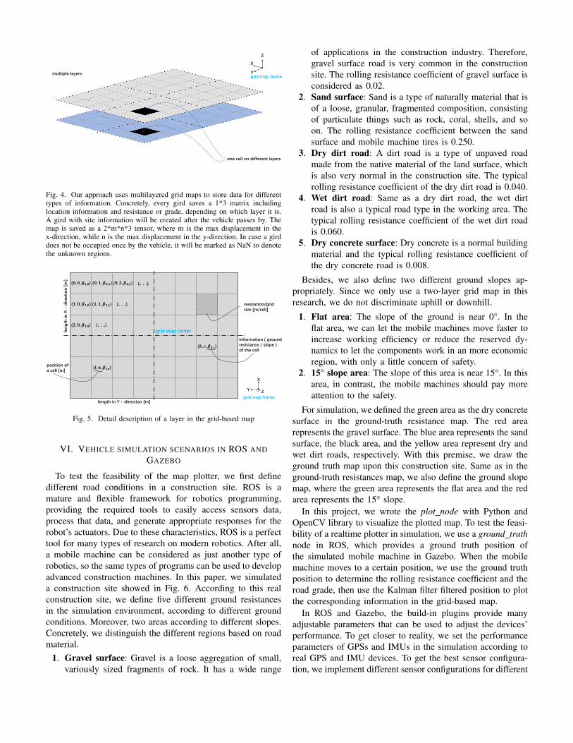
Inspired by the research from Fankhauser [54], a map caninclude many layers to store different types of data informa-tion. Thus, to develop a realtime plotter of the construction siteaccording to ground condition, we use a multi-layer grid-basedmap, which divides the environment into uniform cells. Fig. 4illustrates the multilayered grid map concept, where each celldata is stored on the congruent layers. In this project, sinceresistance and grade of the road are the most of importanceinformation for the construction machines, we adopt a twolayers grid map. Concretely in our study, the map is dividedinto small cells, whose resolution is 1 meter per cell. Aswe discussed in previous section, we use GPS/IMU fusionKalman filter algorithms to locate the mobile machine in theconstruction site.

As can be seen in Fig. 4, to describe the ground condition ofconstruction sites, we use the values of each cell to representthe information of the ground situation. In Fig. 5, a layerthat holds the data of a grid-based map is shown. Obviously,although we only demonstrate the approach with two layers, itis relatively easy to extend the third layer in case that uphill ordownhill is vital, as the third layer is responsible for recordingthe heading of the vehicle.

Based on the previous study, both resistance and gradeof the road can be gathered in realtime. Thus, we assumethat the ground resistance and slope are known after themobile machine passed by. When the mobile machine passesthrough each grid cell, ground information will be added tothe corresponding grid of the two layer-grid-maps. Concretely,the plotting algorithm combines the localization results fromthe Kalman filter and the grade and resistance informationfrom the recursive least square algorithm. To implement theplotting algorithm in ROS, we created a node in ROS that cansubscribe to the localization results from the Kalman filternode and gather the current information from ground truthmaps with the assumption that resistance and grade of theroad can be estimated or measured well.

one cell on different layers

multiple layers

X

Y

Z

grid map frame

Fig. 4. Our approach uses multilayered grid maps to store data for differenttypes of information. Concretely, every gird saves a 1*3 matrix includinglocation information and resistance or grade, depending on which layer it is.A gird with site information will be created after the vehicle passes by. Themap is saved as a 2*m*n*3 tensor, where m is the max displacement in thex-direction, while n is the max displacement in the y-direction. In case a girddoes not be occupied once by the vehicle, it will be marked as NaN to denotethe unknown regions.

(𝟎, 𝟎, 𝜷𝟎,𝟎) (𝟎, 𝟏, 𝜷𝟎,𝟏) (𝟎, 𝟐, 𝜷𝟎,𝟐)

X

Y Z

(𝟏, 𝟎, 𝜷𝟏,𝟎) (𝟏, 𝟏, 𝜷𝟏,𝟏)

(𝟐, 𝟎, 𝜷𝟐,𝟎)

resolution/gridsize [m/cell]

(𝒍, 𝒏, 𝜷𝒍,𝒏)position of a cell [m]

length in Y - direction [m]

len

gth

in

X -

dir

ect

ion

[m

]

(𝒌, 𝒄, 𝜷𝒌,𝒄)

Information ( ground resistance / slope ) of the cell

(. . .)

grid map frame

(. . .)

(. . .)grid map center

Fig. 5. Detail description of a layer in the grid-based map

VI. VEHICLE SIMULATION SCENARIOS IN ROS ANDGAZEBO

To test the feasibility of the map plotter, we first definedifferent road conditions in a construction site. ROS is amature and flexible framework for robotics programming,providing the required tools to easily access sensors data,process that data, and generate appropriate responses for therobot’s actuators. Due to these characteristics, ROS is a perfecttool for many types of research on modern robotics. After all,a mobile machine can be considered as just another type ofrobotics, so the same types of programs can be used to developadvanced construction machines. In this paper, we simulateda construction site showed in Fig. 6. According to this realconstruction site, we define five different ground resistancesin the simulation environment, according to different groundconditions. Moreover, two areas according to different slopes.Concretely, we distinguish the different regions based on roadmaterial.

1. Gravel surface: Gravel is a loose aggregation of small,variously sized fragments of rock. It has a wide range

of applications in the construction industry. Therefore,gravel surface road is very common in the constructionsite. The rolling resistance coefficient of gravel surface isconsidered as 0.02.

2. Sand surface: Sand is a type of naturally material that isof a loose, granular, fragmented composition, consistingof particulate things such as rock, coral, shells, and soon. The rolling resistance coefficient between the sandsurface and mobile machine tires is 0.250.

3. Dry dirt road: A dirt road is a type of unpaved roadmade from the native material of the land surface, whichis also very normal in the construction site. The typicalrolling resistance coefficient of the dry dirt road is 0.040.

4. Wet dirt road: Same as a dry dirt road, the wet dirtroad is also a typical road type in the working area. Thetypical rolling resistance coefficient of the wet dirt roadis 0.060.

5. Dry concrete surface: Dry concrete is a normal buildingmaterial and the typical rolling resistance coefficient ofthe dry concrete road is 0.008.

Besides, we also define two different ground slopes ap-propriately. Since we only use a two-layer grid map in thisresearch, we do not discriminate uphill or downhill.

1. Flat area: The slope of the ground is near 0°. In theflat area, we can let the mobile machines move faster toincrease working efficiency or reduce the reserved dy-namics to let the components work in an more economicregion, with only a little concern of safety.

2. 15° slope area: The slope of this area is near 15°. In thisarea, in contrast, the mobile machines should pay moreattention to the safety.

For simulation, we defined the green area as the dry concretesurface in the ground-truth resistance map. The red arearepresents the gravel surface. The blue area represents the sandsurface, the black area, and the yellow area represent dry andwet dirt roads, respectively. With this premise, we draw theground truth map upon this construction site. Same as in theground-truth resistances map, we also define the ground slopemap, where the green area represents the flat area and the redarea represents the 15° slope.

In this project, we wrote the plot node with Python andOpenCV library to visualize the plotted map. To test the feasi-bility of a realtime plotter in simulation, we use a ground truthnode in ROS, which provides a ground truth position ofthe simulated mobile machine in Gazebo. When the mobilemachine moves to a certain position, we use the ground truthposition to determine the rolling resistance coefficient and theroad grade, then use the Kalman filter filtered position to plotthe corresponding information in the grid-based map.

In ROS and Gazebo, the build-in plugins provide manyadjustable parameters that can be used to adjust the devices’performance. To get closer to reality, we set the performanceparameters of GPSs and IMUs in the simulation according toreal GPS and IMU devices. To get the best sensor configura-tion, we implement different sensor configurations for different

105

2595

120

64

1020

38

80

15

(a) Example construction site divided into five areas according todifferent ground resistances

120

80

9525

64

20

38

40 3030

20

15

(b) Example construction site divided into two areas according todifferent slopes

Fig. 6. The ground truth map with dimensions. The simulation environmentwe used in Gazebo was modeled based on a real construction site, and theparameters are selected according to material characteristics. Since simulatinga small construction site may cause system error and thus lack plausibility,we augmented this real construction site’s dimensions in Gazebo.

algorithms. Each group of sensor configurations is simulatedunder the same condition by rosbag, and the results are outputsimultaneously.

VII. EXPERIMENT AND RESULTS

A. Localization results

To explore the most suitable sensor arrangements of theKalman filter for construction machinery, we compared theresults from different sensor configurations with differentmethods. The concrete sensor arrangements in this project areshown in Tab. I.

To evaluate the performance of the different variants ofsensors and algorithms concerning accurately positioning, wecontrolled the wheel loader to drive on the previously definedconstruction site in Gazebo, and recorded the data fromsensors at the same time. Afterward, the localization results ofthe different methods are compared to the ground truth. Herewe use the root-mean-square error (RMSE) as a quantitativeindicator of the error to assess the pose estimation results.

TABLE ISENSOR CONFIGURATIONS

Group Sensor ( 0 = deactivated, 1 = active ) KFGPS 1 GPS 2 GPS 3 IMU 1 IMU 2 IMU 3 Encoder1 0 0 0 1 0 0 1 EKF2 1 0 0 1 0 0 1 EKF3 1 0 0 1 1 0 1 EKF4 1 0 0 1 1 1 1 EKF5 1 1 0 1 0 0 1 EKF6 1 1 0 1 1 0 1 EKF7 1 1 0 1 1 1 1 EKF8 1 1 1 1 1 1 1 EKF9 0 0 0 1 0 0 1 UKF10 1 0 0 1 0 0 1 UKF11 1 0 0 1 1 0 1 UKF12 1 0 0 1 1 1 1 UKF13 1 1 0 1 0 0 1 UKF14 1 1 0 1 1 0 1 UKF15 1 1 0 1 1 1 1 UKF16 1 1 1 1 1 1 1 UKF

In our simulation, we ignore the mirror difference caused by the slightlydifferent installation position of sensors. Therefore, the various configurationsare reduced from 64 to 16. Since odometry is robust and necessary for manyapplications, we do not consider the case without an encoder.

RMSE =

√∑ni=1 (Si − ˆSi)

2

n(18)

Where ˆS is the vector including estimated x and y position, Sis the denotes ground truth x and y position, n is number ofall estimated samples, and the footnote i denotes the ith timestep.

Fig. 7 shows the wheel loader estimated trajectories givenby different approaches and the ground truth trajectory, wherethe red lines are the ground truth trajectories that the vehiclepasses, and the blue lines are the estimated position of thevehicle. Since only EKF and UKF are capable of handlingthe nonlinear problem, we compare the results obtained usingEKF filtering and the UKF filtering technique with differentsensor arrangements. Notice that, odometry sensor is alwaysused though we do not explicitly mention it. Apparently, theUKF performs better than the EKF, which is also in linewith the conclusion from most studies. Generally speaking,with GPS fusing in the estimation, the accuracy improvesdrastically. Also, since the GPS may lose signal every 10seconds, an additional GPS sensor can surely increase theposition accuracy. In contrast, more IMUs can only slightlyimprove the accuracy of positioning. As we can see, the IMU+ Odometry estimation method yields inferior performance nomatter with EKF or UKF. Once the IMU reports an inaccurateheading, the errors will be accumulated, causing the measuredposition drifts further away from its true position as the wheelloader travels.

Fig. 8 shows a comparison of localization error between thedifferent approaches with respect to time. As shown in Fig.8, the RMSE and the euclidean distance error of each sensorarrangement can be obtained, indicating that the EKF has moresignificant tracking error than UKF. It happens because thelinearization through its Jacobian is an approximation, and thekinematic model of the wheel loader is highly nonlinear. Toget a more intuitive and accurate description of the error for

-60 -40 -20 0 20 40 60 80 100 120

Position X [m]

-40

-30

-20

-10

0

10

20

30

40

50

60P

ositi

on Y

[m]

Net RMSE = 75.3671 m

(a) EKF with only one IMU

-60 -40 -20 0 20 40 60 80 100 120

Position X [m]

-40

-30

-20

-10

0

10

20

30

40

50

60

Pos

ition

Y [m

]

Net RMSE = 65.4774 m

(b) UKF with only one IMU

-50 -40 -30 -20 -10 0 10 20 30 40 50

Position X [m]

-40

-30

-20

-10

0

10

20

30

40

50

60

Pos

ition

Y [m

]

Net RMSE = 3.7363 m

(c) EKF with 1 IMU and 1 GPS

-50 -40 -30 -20 -10 0 10 20 30 40 50

Position X [m]

-40

-30

-20

-10

0

10

20

30

40

50

60

Pos

ition

Y [m

]

Net RMSE = 2,3234 m

(d) UKF with 1 IMU and 1 GPS

-50 -40 -30 -20 -10 0 10 20 30 40 50

Position X [m]

-40

-30

-20

-10

0

10

20

30

40

50

60

Pos

ition

Y [m

]

Net RMSE = 3.2963 m

(e) EKF with 2 IMU and 1 GPS

-50 -40 -30 -20 -10 0 10 20 30 40 50

Position X [m]

-40

-30

-20

-10

0

10

20

30

40

50

60

Pos

ition

Y [m

]

Net RMSE = 2.2781 m

(f) UKF with 2 IMU and 1 GPS

-50 -40 -30 -20 -10 0 10 20 30 40 50

Position X [m]

-40

-30

-20

-10

0

10

20

30

40

50

60

Pos

ition

Y [m

]

Net RMSE = 3.7660 m

(g) EKF with 3 IMU and 1 GPS

-50 -40 -30 -20 -10 0 10 20 30 40 50

Position X [m]

-40

-30

-20

-10

0

10

20

30

40

50

60

Pos

ition

Y [m

]

Net RMSE = 2.5742 m

(h) UKF with 3 IMU and 1 GPS

-50 -40 -30 -20 -10 0 10 20 30 40 50

Position X [m]

-40

-30

-20

-10

0

10

20

30

40

50

60

Pos

ition

Y [m

]

Net RMSE = 2.7474 m

(i) EKF with 1 IMU and 2 GPS

-50 -40 -30 -20 -10 0 10 20 30 40 50

Position X [m]

-40

-30

-20

-10

0

10

20

30

40

50

60

Pos

ition

Y [m

]

Net RMSE = 1.7217 m

(j) UKF with 1 IMU and 2 GPS

-50 -40 -30 -20 -10 0 10 20 30 40 50

Position X [m]

-40

-30

-20

-10

0

10

20

30

40

50

60

Pos

ition

Y [m

]

Net RMSE = 2.6517 m

(k) EKF with 2 IMU and 2 GPS

-50 -40 -30 -20 -10 0 10 20 30 40 50

Position X [m]

-40

-30

-20

-10

0

10

20

30

40

50

60

Pos

ition

Y [m

]

Net RMSE = 1.5460 m

(l) UKF with 2 IMU and 2 GPS

-50 -40 -30 -20 -10 0 10 20 30 40 50

Position X [m]

-40

-30

-20

-10

0

10

20

30

40

50

60

Pos

ition

Y [m

]

Net RMSE = 2.4747 m

(m) EKF with 3 IMU and 2 GPS

-50 -40 -30 -20 -10 0 10 20 30 40 50

Position X [m]

-40

-30

-20

-10

0

10

20

30

40

50

60

Pos

ition

Y [m

]

Net RMSE = 1.4024 m

(n) UKF with 3 IMU and 2 GPS

-50 -40 -30 -20 -10 0 10 20 30 40 50

Position X [m]

-40

-30

-20

-10

0

10

20

30

40

50

60

Pos

ition

Y [m

]

Net RMSE = 2.2980 m

(o) EKF with 3 IMU and 3 GPS

-50 -40 -30 -20 -10 0 10 20 30 40 50

Position X [m]

-40

-30

-20

-10

0

10

20

30

40

50

60

Pos

ition

Y [m

]

Net RMSE = 1.2458 m

(p) UKF with 3 IMU and 3 GPS

Fig. 7. The IMU + Odometry estimation method yields for both EKF and UKF the RMSE over 70 meters. Except for the IMU + Odometry methods, theother results can be divided into four performance levels according to the error scale. The worst level is EKF with one GPS, where the RMSE is about 3 ∼4 m. The second level is EKF with two GPS and EKF with three IMU and three GPS. In these cases, the RMSEs are about 2 ∼ 3 m. A better level is UKFwith 1 GPS and 1 IMU, where the RMSE of the third level can be achieved about 2 ∼ 2.5 m. Finally, our experiment’s best class is UKF with 2 GPS and 1IMU, and UKF with 3 IMU and 3 GPS, which reduce the RMSE to about 1.2 m.

each sensor configuration and method, we create Tab. II todemonstrate the RMSE in detail.

As aforementioned, the GPS signal will be lost for onesecond every ten seconds. Thus, there are some noticeableinstantaneous position changes every ten seconds. The lossof GPS signals clearly causes these jumps. As we can see,for sensor configuration with only one GPS, the leap of thelocalization error as well as the variance values are moresharply. Obviously, with the number of GPS increases, thejumps are diminished and therefore become more acceptable.

Apparently, the simulation results show that UKF is abetter approach using data collected by onboard sensors of

the wheel loader in gazebo environments. Intuitively, moresensors represent higher accuracy. However, the results showthat an appropriate number of sensors can achieve acceptableaccuracy at a lower cost. As we can see in Tab. II, the RMSEof UKF with 1 IMU 2 GPS is 1.7217 m, and UKF with3 IMU and 2 GPS is 1.4024 m. With additional 2 IMUand 1 GPS, the RMSE is only slightly reduced by 0.3 m.More importantly, the maximal error is strongly diminished byone additional GPS, whereas continually increasing the sensornumber does not further reduce the error proportionally. Ofcourse, according to different application scenarios, differentsensor configurations shall be chosen. For our application

30 40 50 60 70 80 90 100 110 120

Time [s]

0

0.5

1

1.5

2

2.5

3

3.5

4

4.5

RM

SE

[m]

EKF 1IMU 1GPSEKF 2IMU 1GPSEKF 3IMU 1GPSEKF 1IMU 2GPSEKF 2IMU 2GPSEKF 3IMU 2GPSEKF 3IMU 3GPS

(a) RMSE of EKF

30 40 50 60 70 80 90 100 110 120

Time [s]

0

0.5

1

1.5

2

2.5

3

3.5

4

4.5

RM

SE

[m]

UKF 1IMU 1GPSUKF 2IMU 1GPSUKF 3IMU 1GPSUKF 1IMU 2GPSUKF 2IMU 2GPSUKF 3IMU 2GPSUKF 3IMU 3GPS

(b) RMSE of UKF

30 40 50 60 70 80 90 100 110 120

Time [s]

0

2

4

6

8

10

12

14

Euc

lidea

n di

stan

ce e

rror

[m]

EKF 1IMU 1GPSEKF 2IMU 1GPSEKF 3IMU 1GPSEKF 1IMU 2GPSEKF 2IMU 2GPSEKF 3IMU 2GPSEKF 3IMU 3GPS

(c) Euclidean distance error of EKF

30 40 50 60 70 80 90 100 110 120

Time [s]

0

2

4

6

8

10

12

Euc

lidea

n di

stan

ce e

rror

[m]

UKF 1IMU 1GPSUKF 2IMU 1GPSUKF 3IMU 1GPSUKF 1IMU 2GPSUKF 2IMU 2GPSUKF 3IMU 2GPSUKF 3IMU 3GPS

(d) Euclidean distance error of UKF

Fig. 8. Quantitative evaluation of different methods. Here (a) and (b) show the accumulative error, i.e., RMSE, while (c) and (d) demonstrate the currentEuclidean distance error of each sensor arrangement. There are some noticeable instantaneous position changes every ten seconds due to infrequent GPSsignal loss. Generally, UKF shows better performance than EKF for both RMSE and euclidean distance error.

TABLE IILOCALIZATION ERRORS OF EACH APPROACH

Group RMSE (m) Net RMSE(m)(x,y)1 (EKF 1 IMU) (69.122, 30.039) 75.3671

2 (EKF 1 IMU 1 GPS) (2.472, 2.802) 3.73633 (EKF 2 IMU 1 GPS) (2.172, 2.480) 3.29634 (EKF 3 IMU 1 GPS) (2.474, 2.840) 3.76605 (EKF 1 IMU 2 GPS) (1.830, 2.050) 2.74746 (EKF 2 IMU 2 GPS) (1.778, 1.968) 2.65177 (EKF 3 IMU 2 GPS) (1.894, 1.593) 2.47478 (EKF 3 IMU 3 GPS) (1.794, 1.437) 2.2980

9 (UKF 1 IMU) (56.586, 32.944) 65.477410 (UKF 1 IMU 1 GPS) (1.654, 1.632) 2.323411 (UKF 2 IMU 1 GPS) (1.374, 1.817) 2.278112 (UKF 3 IMU 1 GPS) (1.611, 2.001) 2.574213 (UKF 1 IMU 2 GPS) (1.093, 1.330) 1.721714 (UKF 2 IMU 2 GPS) (0.975, 1.200) 1.546015 (UKF 3 IMU 2 GPS) (0.873, 1.098) 1.402416 (UKF 3 IMU 3 GPS) (0.826, 0.933) 1.2458

scenario, UKF with 1 IMU and 2 GPS has sufficient accuracyand a better economy respecting sensor hardware cost and

onboard ECU computational effort. Thus, we suggest usingthis sensor configuration to locate the mobile machines andthen develop the realtime map plotter.

B. Plotter results

As our ultimate goal is to create a map of the currentworking site in realtime based on localization technology sothat corresponding optimization can then be achieved, theground truth maps and estimated maps with different sensorconfigurations coupled with various algorithms are shown andcompared in Fig. 9. Since we use a two-layer grid map,both rolling friction coefficient and road grade are recordedand used to create the estimated maps. In our study, theground information are saved in corresponding grid after thewheel loader passes by and identify the ground informationsuch as friction and slope through the specific algorithm,e.g. recursive least square. As aforementioned, to locate themobile machine’s position in a cost-efficient fashion, we

(a) Predefined five areas of resis-tance plotted by OpenCV

(b) Result of ground resistance mapwith wheel loader (EKF with 1 IMUand 1 GPS)

(c) Result of ground resistance mapwith wheel loader (UKF with 1 IMUand 1 GPS)

(d) Result of ground resistance mapwith wheel loader (UKF with 1 IMUand 2 GPS)

(e) Predefined two areas of roadgrade plotted by OpenCV

(f) Result of road grade map withwheel loader (EKF with 1 IMU and1 GPS)

(g) Result of road grade map withwheel loader (UKF with 1 IMU and1 GPS)

(h) Result of road grade map withwheel loader (UKF with 1 IMU and2 GPS)

Fig. 9. The ground truth and estimated maps. In the ground resistance map and road grade map plotted by EKF with 1 IMU and 1 GPS, the spikes causedby infrequent GPS are quite obvious. With additional GPS sensor fused in Kalman filter, the spikes improve a lot.

(a) Result of EKF with 1 IMU and 1 GPS (b) Result of UKF with 1 IMU and 1 GPS (c) Result of UKF with 1 IMU and 2 GPS

(d) Result of EKF with 1 IMU and 1 GPS (e) Result of UKF with 1 IMU and 1 GPS (f) Result of UKF with 1 IMU and 2 GPS

Fig. 10. Difference between ground truth and the estimated map. Here we compare the predefined areas and the plotted path, where the white pixels are thewrong plotted grids. (a),(b),(c) are the Friction map results, and (d),(e),(f) are the road grade map results. UKF shows more accurate positioning capabilitiesthan EKF, and with two GPS fused in the Kalman filter, the wrong located grid is less than just with one GPS signal.

adopt the configuration of the UKF with 1 IMU and 2 GPS.Also, in order to compare the performance of the selectedconfiguration, we draw the results of the EKF with 1 IMU and1 GPS and the UKF with 1 IMU and 1 GPS as the controlgroups. The mispredicted points are calculated as described in(19),

Er,s =

m,n∑i=1,j=1

ei,j =

1, if q(Gi,j = Gi,j)∩q(Gi,j = NaN)

0, if (Gi,j = Gi,j)∩q(Gi,j = NaN)

0, if Gi,j = NaN(19)

where Gi,j denotes the estimated grid map information, Gi,j

is the ground truth map information, E is the accumulatednumber of errors, the subscript r and s denotes resistance andslope map, respectively. Obviously, the goal is to minimize thepercent of mispredicted points versus total predicted points,described as (20),

min Jr,s =Er,s

T(20)

where T is the total estimated number, and J is the quantitativecriteria to evaluate the accuracy of the plotted map.

The localization errors of each group are shown in Tab.III, where we can see the necessity of the introduction of thesecond GPS sensors, and the adoption of unscented Kalmanfilter.

TABLE IIILOCALIZATION ERRORS OF EACH APPROACH DURING THE PLOTTING

Group RMSE (m) Net RMSE(m)(x,y)1 (EKF 1 IMU 1 GPS) (2.584, 3.407) 4.44442 (UKF 1 IMU 1 GPS) (2.003, 2.314) 3.06033 (UKF 1 IMU 2 GPS) (1.336, 1.533) 2.0334

To evaluate the plotted maps’ accuracy, we use Matlabto implement an algorithm to compare the predefined areaand the plotted path the mobile machine traveled. Fig. 10graphically illustrate the mispredicted grid point with whitecolor, where the mispredicted points are generally distributedin the marginal zone. This is because even the localizationtechnology makes some mistakes; the problem is unlikely tocause an error as long as the vehicle is not at the very edgeof different zones, indicating the robustness of this mappingidea of the construction site.

After calculating the wrong located grids and all the plottedgrids and according to the Eq. (19) and (20):

1. For EKF with 1 IMU and 1 GPS: an error rate Jr =2.389% of the ground resistances map and an error rateJs = 2.258% of the slope map can be obtained.

2. For UKF with 1 IMU and 1 GPS: an error rate Jr =1.482% of the ground resistances map and an error rateJs = 1.682% of the slope map can be obtained.

3. For UKF with 1 IMU and 2 GPS: an error rate Jr =0.997% of the ground resistances map and an error rateJs = 1.223% of the slope map can be obtained.

VIII. CONCLUSION

In this study, we proposed an approach to creating amulti-layer map of the construction site in realtime so thatthe environmental information can be taken into account toimprove vehicle efficiency and safety further or contribute tothe path planning of mobile machines in the construction site.Considering the common phenomenon in reality mentioned byother researchers, such as noisy sensors and infrequent signalloss, we set up our simulation environment in Gazebo witha ROS package based on a real construction site. Accordingto our tests in Gazebo by implementing a series of sensorconfigurations, we found that the configuration that 1 IMU

and 2 GPS with encoder using UKF has the best for overallperformance with respect to accuracy and cost. By comparingthe estimated maps drawn by map plotter and the predefinedmaps, the errors are only 1.0% and 1.2% for road resistantforce and grade, separately. Thus, we believe that the devel-oped plotter can be used to save the road condition in realtimewithin a reasonable error range and encourage the engineer inconstruction machines to develop novel algorithms to furtherimprove the holistic performance of machines based on ourapproach.

A. Outlook

In our research, we show the method to create a mapwith only one mobile machine. However, in a real workingsite, many mobile machines work simultaneously on theconstruction site, indicating the possibility of creating a mapeven faster if the machines can share the information. Thus,we encourage the researchers to enable the cooperative mapdrawing approach by means of WIFI or 5G.

REFERENCES

[1] P. V. Osinenko, M. Geissler, and T. Herlitzius, “A method of optimaltraction control for farm tractors with feedback of drive torque,” Biosys-tems Engineering, vol. 129, pp. 20–33, 2015.

[2] M. W. Sprengel, “Influence of architecture design on the performanceand fuel efficiency of hydraulic hybrid transmissions,” Dissertations,Purdue University, West Lafayette, 2015.

[3] M. Vukovic, S. Sgro, and H. Murrenhoff, “Steam - a mobile hydraulicsystem with engine integration,” in ASME/BATH 2013 Symposium onFluid Power and Motion Control, Sarasota, 2013, pp. V001T01A005–V001T01A005.

[4] M. Vukovic, R. Leifeld, and H. Murrenhoff, “Steam – a hydraulichybrid architecture for excavators,” in 10th International Fluid PowerConference. Dresden: Technische Universitat Dresden, 2016, pp. 151–162.

[5] Y. Xiang, R. Li, C. Brach, X. Liu, and M. Geimer, “A novel algorithmfor hydrostatic-mechanical mobile machines with a dual-clutch trans-mission,” in 11th IEEE Global Fluid Power Society PhD Symposium,Guilin, China, 2020.

[6] L. Ge, L. Quan, X. Zhang, B. Zhao, and J. Yang, “Efficiency im-provement and evaluation of electric hydraulic excavator with speed anddisplacement variable pump,” Energy Conversion and Management, vol.150, pp. 62–71, 2017.

[7] L. Ge, L. Quan, X. Zhang, J. Huang, and B. Zhao, “High energyefficiency driving of the hydraulic excavator boom with an asymmetricpump,” in Fluid power networks : proceedings : 19th - 21th March 2018: 11th International Fluid Power Conference, Aachen, 2018.

[8] S. Joos, A. Trachte, M. Bitzer, and K. Graichen, “Constrained real-time control of hydromechanical powertrains-methodology and practicalapplication,” Mechatronics, vol. 71, p. 102397, 2020.

[9] Y. Xiang and M. Geimer, “Optimization of operation startegy forprimary torque based hydrostatic drivetrain using artificial intelligence,”in Fluid power networks : proceedings : 12th International Fluid PowerConference, 2020.

[10] S. Mutschler, N. Brix, and Y. Xiang, “Torque control for mobile ma-chines,” in 11th International Fluid Power Conference, H. Murrenhoff,Ed. Aachen: RWTH Publications, 2018, pp. 186–195.

[11] Y. Xiang, Q. Cui, T. Su, C. Brach, and M. Geimer, “Mass and gradeestimation of mobile machines,” arXiv, 2020.

[12] A. Vahidi, A. Stefanopoulou, and H. Peng, “Recursive least squares withforgetting for online estimation of vehicle mass and road grade: theoryand experiments,” Vehicle System Dynamics, vol. 43, no. 1, pp. 31–55,2005.

[13] Y. Xiang, B. Xu, T. Su, C. Brach, S. Mao, and M. Geimer, “5g meetsconstruction machines: Towards a smart working site,” arXiv, 2020.

[14] H. Tan and J. Huang, “Dgps-based vehicle-to-vehicle cooperative col-lision warning: Engineering feasibility viewpoints,” IEEE Transactionson Intelligent Transportation Systems, vol. 7, no. 4, pp. 415–428, 2006.

[15] R. E. Kalman, “A new approach to linear filtering and predictionproblems,” Transactions of the ASME–Journal of Basic Engineering,vol. 82, pp. 35–45, 1960.

[16] S. Jung, J. Kim, and S. Kim, Eds., Simultaneous localization andmapping of a wheel-based autonomous vehicle with ultrasonic sensors,vol. 14, 2009.

[17] S. Wang, Z. Deng, and G. Yin, “An accurate gps-imu/dr data fusionmethod for driverless car based on a set of predictive models and gridconstraints,” Sensors (Basel, Switzerland), vol. 16, no. 3, p. 280, 2016.

[18] D. Perea, J. Hernandez-Aceituno, A. Morell, J. Toledo, A. Hamilton, andL. Acosta, “Mcl with sensor fusion based on a weighting mechanismversus a particle generation approach,” in 16th International IEEEConference on Intelligent Transportation Systems (ITSC 2013), 2013,pp. 166–171.

[19] S. Sukkarieh, E. M. Nebot, and H. F. Durrant-Whyte, “A high integrityimu/gps navigation loop for autonomous land vehicle applications,”IEEE Transactions on Robotics and Automation, vol. 15, no. 3, pp.572–578, 1999.

[20] S. Iwataki, H. Fujii, A. Moro, A. Yamashita, H. Asama, and H. Yoshi-nada, “Visualization of the surrounding environment and operational partin a 3dcg model for the teleoperation of construction machines,” in 2015IEEE/SICE International Symposium on System Integration (SII). IEEE,2015, pp. 81–87.

[21] I. Skog and P. Handel, “In-car positioning and navigation technologies—a survey,” IEEE Transactions on Intelligent Transportation Systems,vol. 10, no. 1, pp. 4–21, 2009.

[22] H. L. Isa, S. A. Saad, A. Hisham, and M. Ishak, “Improvement of gpsaccuracy in positioning by using dgps technique,” in Modeling, Designand Simulation of Systems, M. S. Mohamed A., H. Wahid, N. A. MohdSubha, S. Sahlan, M. A. Md. Yunus, and A. R. Wahap, Eds. Singapore:Springer Singapore, 2017, pp. 3–11.

[23] J. Kim, J. Song, H. No, D. Han, D. Kim, B. Park, and C. Kee, “Accu-racy improvement of dgps for low-cost single-frequency receiver usingmodified flachen korrektur parameter correction,” ISPRS InternationalJournal of Geo-Information, vol. 6, no. 7, p. 222, 2017.

[24] E. Zhang and N. Masoud, “Increasing gps localization accuracy with re-inforcement learning,” IEEE Transactions on Intelligent TransportationSystems, pp. 1–12, 2020.

[25] G. Soatti, M. Nicoli, N. Garcia, B. Denis, R. Raulefs, and H. Wymeersch,“Implicit cooperative positioning in vehicular networks,” IEEE Transac-tions on Intelligent Transportation Systems, vol. 19, no. 12, pp. 3964–3980, 2018.

[26] M. Skoglund, T. Petig, B. Vedder, H. Eriksson, and E. M. Schiller,“Static and dynamic performance evaluation of low-cost rtk gps re-ceivers,” in 2016 IEEE Intelligent Vehicles Symposium (IV). IEEE,2016, pp. 16–19.

[27] J. Toledo, J. D. Pineiro, R. Arnay, D. Acosta, and L. Acosta, “Improvingodometric accuracy for an autonomous electric cart,” Sensors (Basel,Switzerland), vol. 18, no. 1, 2018.

[28] X. Qi, W. Wang, M. Yuan, Y. Wang, M. Li, L. Xue, and Y. Sun,“Building semantic grid maps for domestic robot navigation,” Inter-national Journal of Advanced Robotic Systems, vol. 17, no. 1, p.172988141990006, 2020.

[29] S. J. Julier and J. K. Uhlmann, “New extension of the kalman filterto nonlinear systems,” in Signal Processing, Sensor Fusion, and TargetRecognition VI, ser. SPIE Proceedings, I. Kadar, Ed. SPIE, 1997, p.182.

[30] E. A. Wan and R. van der Merwe, “The unscented kalman filter for non-linear estimation,” in Proceedings of the IEEE 2000 Adaptive Systemsfor Signal Processing, Communications, and Control Symposium (Cat.No.00EX373). IEEE, 2000, pp. 153–158.

[31] G. Welch and G. Bishop, “An introduction to the kalman filter,” 1995.[32] L. C. Bento, U. Nunes, F. Moita, and A. Surrecio, “Sensor fusion for

precise autonomous vehicle navigation in outdoor semi-structured envi-ronments,” in IEEE Conference on Intelligent Transportation Systems,2005, pp. 245–250.

[33] F. Zhang, H. Stahle, G. Chen, C. Chen, C. Simon, C. Buckl, andA. Knoll, “A sensor fusion approach for localization with cumulativeerror elimination,” in 2012 IEEE International Conference on Multi-sensor Fusion and Integration for Intelligent Systems (MFI), 2012, pp.1–6.

[34] C. Li, B. Dai, and T. Wu, “Vision-based precision vehicle localizationin urban environments,” in 2013 Chinese Automation Congress, 2013,pp. 599–604.

[35] R. W. Wolcott and R. M. Eustice, “Visual localization within lidarmaps for automated urban driving,” in 2014 IEEE/RSJ InternationalConference on Intelligent Robots and Systems, 2014, pp. 176–183.

[36] E. Ward and J. Folkesson, “Vehicle localization with low cost radarsensors,” in 2016 IEEE Intelligent Vehicles Symposium (IV), 2016, pp.864–870.

[37] A. Y. Hata and D. F. Wolf, “Feature detection for vehicle localizationin urban environments using a multilayer lidar,” IEEE Transactions onIntelligent Transportation Systems, vol. 17, no. 2, pp. 420–429, 2016.

[38] J. A. del Peral-Rosado, J. A. Lopez-Salcedo, S. Kim, and G. Seco-Granados, “Feasibility study of 5g-based localization for assisted driv-ing,” in 2016 International Conference on Localization and GNSS (ICL-GNSS). IEEE, 2016, pp. 1–6.

[39] M. Rohani, D. Gingras, V. Vigneron, and D. Gruyer, “A new decen-tralized bayesian approach for cooperative vehicle localization based onfusion of gps and vanet based inter-vehicle distance measurement,” IEEEIntelligent Transportation Systems Magazine, vol. 7, no. 2, pp. 85–95,2015.

[40] S. Kuutti, S. Fallah, K. Katsaros, M. Dianati, F. Mccullough, andA. Mouzakitis, “A survey of the state-of-the-art localization techniquesand their potentials for autonomous vehicle applications,” IEEE Internetof Things Journal, vol. 5, no. 2, pp. 829–846, 2018.

[41] J. Larsson, M. Broxvall, and A. Saffiotti, “An evaluation of localautonomy applied to teleoperated vehicles in underground mines,” in2010 IEEE International Conference on Robotics and Automation, 2010,pp. 1745–1752.

[42] J. M. Roberts, E. S. Duff, and P. I. Corke, “Reactive navigation andopportunistic localization for autonomous underground mining vehicles,”Information Sciences, vol. 145, no. 1-2, pp. 127–146, 2002,.

[43] R. Gu, R. Marinescu, C. Seceleanu, and K. Lundqvist, “Formal veri-fication of an autonomous wheel loader by model checking,” in 2018ACM/IEEE Conference on Formal Methods in Software Engineering,2018, pp. 74–83.

[44] Y. Xiang, T. Tang, T. Su, C. Brach, L. Liu, S. Mao, and M. Geimer,“Fast crdnn: Towards on site training of mobile construction machines,”arXiv, 2020. [Online]. Available: https://arxiv.org/pdf/2006.03169.pdf

[45] S. Bang, F. Baek, S. Park, W. Kim, and H. Kim, “An image augmentationmethod for detecting construction resources using convolutional neuralnetwork and uav images,” in 36th International Symposium on Automa-tion and Robotics in Construction, M. Al-Hussein, Ed. InternationalAssociation for Automation and Robotics in Construction (IAARC),2019.

[46] Z. Shang and Z. Shen, “Real-time 3d reconstruction on constructionsite using visual slam and uav,” 2019. [Online]. Available:arXivpreprintarXiv:1712.07122

[47] Q. Zhou, J. Li, B. Shuai, H. Williams, Y. He, Z. Li, H. Xu, and F. Yan,“Multi-step reinforcement learning for model-free predictive energymanagement of an electrified off-highway vehicle,” Applied Energy, vol.255, p. 113755, 2019.

[48] Q. Zhou, Y. Zhang, Z. Li, J. Li, H. Xu, and O. Olatunbosun, “Cyber-physical energy-saving control for hybrid aircraft-towing tractor basedon online swarm intelligent programming,” IEEE Transactions on In-dustrial Informatics, vol. 14, no. 9, pp. 4149–4158, 2017.

[49] Y. Xiang, S. Mutschler, N. Brix, C. Brach, and M. Geimer, “Optimizationof hydrostatic-mechanical transmission control strategy by means oftorque control,” in Fluid power networks : proceedings : 12th Inter-national Fluid Power Conference, 2020.

[50] Y. Xiang, H. Wang, T. Su, R. Li, C. Brach, S. Mao, and M. Geimer,“Kit moma: A mobile machines dataset,” arXiv, 2020. [Online].Available: arXiv:2007.04198

[51] F. Samie, L. Bauer, and J. Henkel, “Iot technologies for embeddedcomputing: A survey,” in 2016 International Conference on Hard-ware/Software Codesign and System Synthesis (CODES+ ISSS). IEEE,2016, pp. 1–10.

[52] Y. Xiang, T. Su, C. Brach, X. Liu, and M. Geimer, “Realtime estimationof ieee 802.11p for mobile working machines communication respectingdelay and packet loss,” in IEEE Intelligent Vehicle Symposium 2020, LasVegas, USA, 2020.

[53] T. Moore and D. Stouch, “A generalized extended kalman filter imple-mentation for the robot operating system,” in Intelligent autonomoussystems 13. Cham: Springer, 2016, pp. 335–348.

[54] P. Fankhauser and M. Hutter, “A universal grid map library: Implemen-tation and use case for rough terrain navigation,” in Robot OperatingSystem (ROS). Springer, 2016, vol. 625, pp. 99–120.