Neural Turing Machines

Alex Graves gravesa@google.com

Greg Wayne gregwayne@google.com

Ivo Danihelka danihelka@google.com

Google DeepMind, London, UK

Abstract

We extend the capabilities of neural networks by coupling them to external memory re-sources, which they can interact with by attentional processes. The combined system isanalogous to a Turing Machine or Von Neumann architecture but is differentiable end-to-end, allowing it to be efficiently trained with gradient descent. Preliminary results demon-strate that Neural Turing Machines can infer simple algorithms such as copying, sorting,and associative recall from input and output examples.

1 IntroductionComputer programs make use of three fundamental mechanisms: elementary operations(e.g., arithmetic operations), logical flow control (branching), and external memory, whichcan be written to and read from in the course of computation (Von Neumann, 1945). De-spite its wide-ranging success in modelling complicated data, modern machine learninghas largely neglected the use of logical flow control and external memory.

Recurrent neural networks (RNNs) stand out from other machine learning methodsfor their ability to learn and carry out complicated transformations of data over extendedperiods of time. Moreover, it is known that RNNs are Turing-Complete (Siegelmann andSontag, 1995), and therefore have the capacity to simulate arbitrary procedures, if properlywired. Yet what is possible in principle is not always what is simple in practice. Wetherefore enrich the capabilities of standard recurrent networks to simplify the solution ofalgorithmic tasks. This enrichment is primarily via a large, addressable memory, so, byanalogy to Turing’s enrichment of finite-state machines by an infinite memory tape, we

1

arX

iv:1

410.

5401

v2 [

cs.N

E]

10

Dec

201

4

dub our device a “Neural Turing Machine” (NTM). Unlike a Turing machine, an NTMis a differentiable computer that can be trained by gradient descent, yielding a practicalmechanism for learning programs.

In human cognition, the process that shares the most similarity to algorithmic operationis known as “working memory.” While the mechanisms of working memory remain some-what obscure at the level of neurophysiology, the verbal definition is understood to meana capacity for short-term storage of information and its rule-based manipulation (Badde-ley et al., 2009). In computational terms, these rules are simple programs, and the storedinformation constitutes the arguments of these programs. Therefore, an NTM resemblesa working memory system, as it is designed to solve tasks that require the application ofapproximate rules to “rapidly-created variables.” Rapidly-created variables (Hadley, 2009)are data that are quickly bound to memory slots, in the same way that the number 3 and thenumber 4 are put inside registers in a conventional computer and added to make 7 (Minsky,1967). An NTM bears another close resemblance to models of working memory since theNTM architecture uses an attentional process to read from and write to memory selectively.In contrast to most models of working memory, our architecture can learn to use its workingmemory instead of deploying a fixed set of procedures over symbolic data.

The organisation of this report begins with a brief review of germane research on work-ing memory in psychology, linguistics, and neuroscience, along with related research inartificial intelligence and neural networks. We then describe our basic contribution, a mem-ory architecture and attentional controller that we believe is well-suited to the performanceof tasks that require the induction and execution of simple programs. To test this architec-ture, we have constructed a battery of problems, and we present their precise descriptionsalong with our results. We conclude by summarising the strengths of the architecture.

2 Foundational Research

2.1 Psychology and NeuroscienceThe concept of working memory has been most heavily developed in psychology to explainthe performance of tasks involving the short-term manipulation of information. The broadpicture is that a “central executive” focuses attention and performs operations on data in amemory buffer (Baddeley et al., 2009). Psychologists have extensively studied the capacitylimitations of working memory, which is often quantified by the number of “chunks” ofinformation that can be readily recalled (Miller, 1956).1 These capacity limitations leadtoward an understanding of structural constraints in the human working memory system,but in our own work we are happy to exceed them.

In neuroscience, the working memory process has been ascribed to the functioning of asystem composed of the prefrontal cortex and basal ganglia (Goldman-Rakic, 1995). Typ-

1There remains vigorous debate about how best to characterise capacity limitations (Barrouillet et al.,2004).

2

ical experiments involve recording from a single neuron or group of neurons in prefrontalcortex while a monkey is performing a task that involves observing a transient cue, waitingthrough a “delay period,” then responding in a manner dependent on the cue. Certain taskselicit persistent firing from individual neurons during the delay period or more complicatedneural dynamics. A recent study quantified delay period activity in prefrontal cortex for acomplex, context-dependent task based on measures of “dimensionality” of the populationcode and showed that it predicted memory performance (Rigotti et al., 2013).

Modeling studies of working memory range from those that consider how biophysicalcircuits could implement persistent neuronal firing (Wang, 1999) to those that try to solveexplicit tasks (Hazy et al., 2006) (Dayan, 2008) (Eliasmith, 2013). Of these, Hazy et al.’smodel is the most relevant to our work, as it is itself analogous to the Long Short-TermMemory architecture, which we have modified ourselves. As in our architecture, Hazyet al.’s has mechanisms to gate information into memory slots, which they use to solve amemory task constructed of nested rules. In contrast to our work, the authors include nosophisticated notion of memory addressing, which limits the system to storage and recallof relatively simple, atomic data. Addressing, fundamental to our work, is usually leftout from computational models in neuroscience, though it deserves to be mentioned thatGallistel and King (Gallistel and King, 2009) and Marcus (Marcus, 2003) have argued thataddressing must be implicated in the operation of the brain.

2.2 Cognitive Science and LinguisticsHistorically, cognitive science and linguistics emerged as fields at roughly the same timeas artificial intelligence, all deeply influenced by the advent of the computer (Chomsky,1956) (Miller, 2003). Their intentions were to explain human mental behaviour based oninformation or symbol-processing metaphors. In the early 1980s, both fields consideredrecursive or procedural (rule-based) symbol-processing to be the highest mark of cogni-tion. The Parallel Distributed Processing (PDP) or connectionist revolution cast aside thesymbol-processing metaphor in favour of a so-called “sub-symbolic” description of thoughtprocesses (Rumelhart et al., 1986).

Fodor and Pylyshyn (Fodor and Pylyshyn, 1988) famously made two barbed claimsabout the limitations of neural networks for cognitive modeling. They first objected thatconnectionist theories were incapable of variable-binding, or the assignment of a particulardatum to a particular slot in a data structure. In language, variable-binding is ubiquitous;for example, when one produces or interprets a sentence of the form, “Mary spoke to John,”one has assigned “Mary” the role of subject, “John” the role of object, and “spoke to” therole of the transitive verb. Fodor and Pylyshyn also argued that neural networks with fixed-length input domains could not reproduce human capabilities in tasks that involve process-ing variable-length structures. In response to this criticism, neural network researchersincluding Hinton (Hinton, 1986), Smolensky (Smolensky, 1990), Touretzky (Touretzky,1990), Pollack (Pollack, 1990), Plate (Plate, 2003), and Kanerva (Kanerva, 2009) inves-tigated specific mechanisms that could support both variable-binding and variable-length

3

structure within a connectionist framework. Our architecture draws on and potentiates thiswork.

Recursive processing of variable-length structures continues to be regarded as a hall-mark of human cognition. In the last decade, a firefight in the linguistics community stakedseveral leaders of the field against one another. At issue was whether recursive processingis the “uniquely human” evolutionary innovation that enables language and is specialized tolanguage, a view supported by Fitch, Hauser, and Chomsky (Fitch et al., 2005), or whethermultiple new adaptations are responsible for human language evolution and recursive pro-cessing predates language (Jackendoff and Pinker, 2005). Regardless of recursive process-ing’s evolutionary origins, all agreed that it is essential to human cognitive flexibility.

2.3 Recurrent Neural NetworksRecurrent neural networks constitute a broad class of machines with dynamic state; thatis, they have state whose evolution depends both on the input to the system and on thecurrent state. In comparison to hidden Markov models, which also contain dynamic state,RNNs have a distributed state and therefore have significantly larger and richer memoryand computational capacity. Dynamic state is crucial because it affords the possibility ofcontext-dependent computation; a signal entering at a given moment can alter the behaviourof the network at a much later moment.

A crucial innovation to recurrent networks was the Long Short-Term Memory (LSTM)(Hochreiter and Schmidhuber, 1997). This very general architecture was developed for aspecific purpose, to address the “vanishing and exploding gradient” problem (Hochreiteret al., 2001a), which we might relabel the problem of “vanishing and exploding sensitivity.”LSTM ameliorates the problem by embedding perfect integrators (Seung, 1998) for mem-ory storage in the network. The simplest example of a perfect integrator is the equationx(t + 1) = x(t) + i(t), where i(t) is an input to the system. The implicit identity matrixIx(t) means that signals do not dynamically vanish or explode. If we attach a mechanismto this integrator that allows an enclosing network to choose when the integrator listens toinputs, namely, a programmable gate depending on context, we have an equation of theform x(t + 1) = x(t) + g(context)i(t). We can now selectively store information for anindefinite length of time.

Recurrent networks readily process variable-length structures without modification. Insequential problems, inputs to the network arrive at different times, allowing variable-length or composite structures to be processed over multiple steps. Because they nativelyhandle variable-length structures, they have recently been used in a variety of cognitiveproblems, including speech recognition (Graves et al., 2013; Graves and Jaitly, 2014), textgeneration (Sutskever et al., 2011), handwriting generation (Graves, 2013) and machinetranslation (Sutskever et al., 2014). Considering this property, we do not feel that it is ur-gent or even necessarily valuable to build explicit parse trees to merge composite structuresgreedily (Pollack, 1990) (Socher et al., 2012) (Frasconi et al., 1998).

Other important precursors to our work include differentiable models of attention (Graves,

4

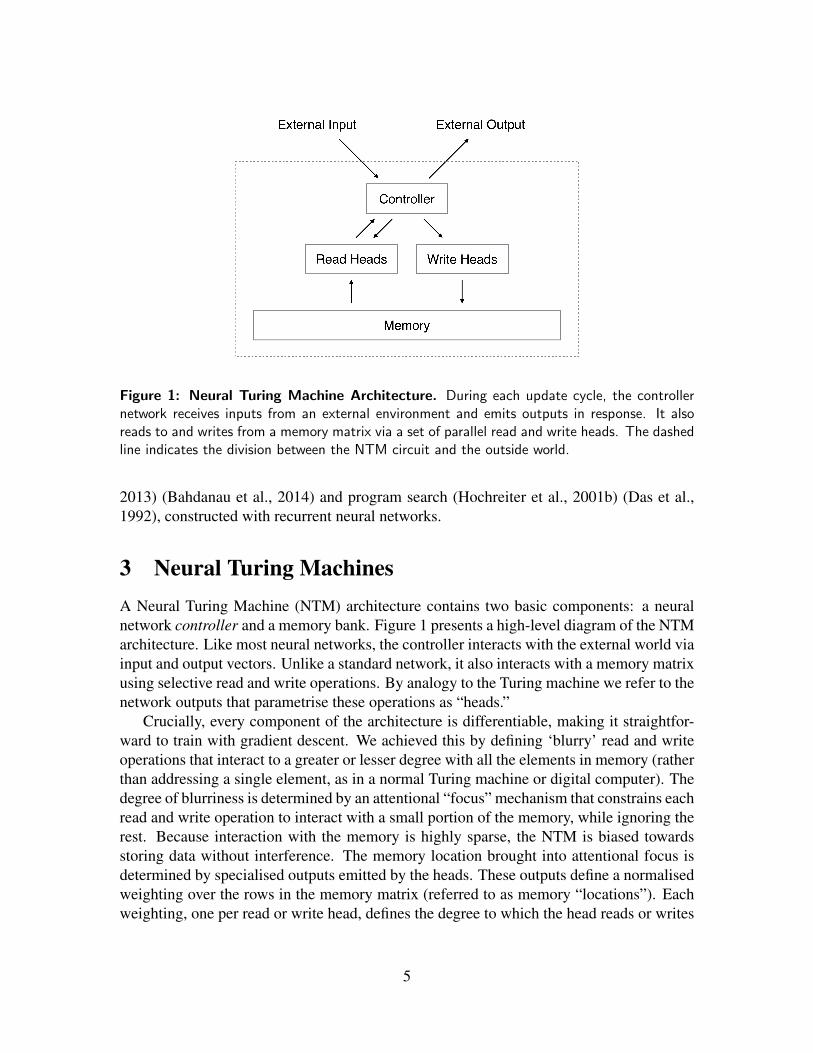
Figure 1: Neural Turing Machine Architecture. During each update cycle, the controllernetwork receives inputs from an external environment and emits outputs in response. It alsoreads to and writes from a memory matrix via a set of parallel read and write heads. The dashedline indicates the division between the NTM circuit and the outside world.

2013) (Bahdanau et al., 2014) and program search (Hochreiter et al., 2001b) (Das et al.,1992), constructed with recurrent neural networks.

3 Neural Turing MachinesA Neural Turing Machine (NTM) architecture contains two basic components: a neuralnetwork controller and a memory bank. Figure 1 presents a high-level diagram of the NTMarchitecture. Like most neural networks, the controller interacts with the external world viainput and output vectors. Unlike a standard network, it also interacts with a memory matrixusing selective read and write operations. By analogy to the Turing machine we refer to thenetwork outputs that parametrise these operations as “heads.”

Crucially, every component of the architecture is differentiable, making it straightfor-ward to train with gradient descent. We achieved this by defining ‘blurry’ read and writeoperations that interact to a greater or lesser degree with all the elements in memory (ratherthan addressing a single element, as in a normal Turing machine or digital computer). Thedegree of blurriness is determined by an attentional “focus” mechanism that constrains eachread and write operation to interact with a small portion of the memory, while ignoring therest. Because interaction with the memory is highly sparse, the NTM is biased towardsstoring data without interference. The memory location brought into attentional focus isdetermined by specialised outputs emitted by the heads. These outputs define a normalisedweighting over the rows in the memory matrix (referred to as memory “locations”). Eachweighting, one per read or write head, defines the degree to which the head reads or writes

5

at each location. A head can thereby attend sharply to the memory at a single location orweakly to the memory at many locations.

3.1 ReadingLet Mt be the contents of the N ×M memory matrix at time t, where N is the numberof memory locations, and M is the vector size at each location. Let wt be a vector ofweightings over the N locations emitted by a read head at time t. Since all weightings arenormalised, the N elements wt(i) of wt obey the following constraints:∑

i

wt(i) = 1, 0 ≤ wt(i) ≤ 1, ∀i. (1)

The length M read vector rt returned by the head is defined as a convex combination ofthe row-vectors Mt(i) in memory:

rt ←−∑i

wt(i)Mt(i), (2)

which is clearly differentiable with respect to both the memory and the weighting.

3.2 WritingTaking inspiration from the input and forget gates in LSTM, we decompose each write intotwo parts: an erase followed by an add.

Given a weighting wt emitted by a write head at time t, along with an erase vectoret whose M elements all lie in the range (0, 1), the memory vectors Mt−1(i) from theprevious time-step are modified as follows:

M̃t(i)←−Mt−1(i) [1− wt(i)et] , (3)

where 1 is a row-vector of all 1-s, and the multiplication against the memory location actspoint-wise. Therefore, the elements of a memory location are reset to zero only if both theweighting at the location and the erase element are one; if either the weighting or the eraseis zero, the memory is left unchanged. When multiple write heads are present, the erasurescan be performed in any order, as multiplication is commutative.

Each write head also produces a lengthM add vector at, which is added to the memoryafter the erase step has been performed:

Mt(i)←− M̃t(i) + wt(i) at. (4)

Once again, the order in which the adds are performed by multiple heads is irrelevant. Thecombined erase and add operations of all the write heads produces the final content of thememory at time t. Since both erase and add are differentiable, the composite write oper-ation is differentiable too. Note that both the erase and add vectors have M independentcomponents, allowing fine-grained control over which elements in each memory locationare modified.

6

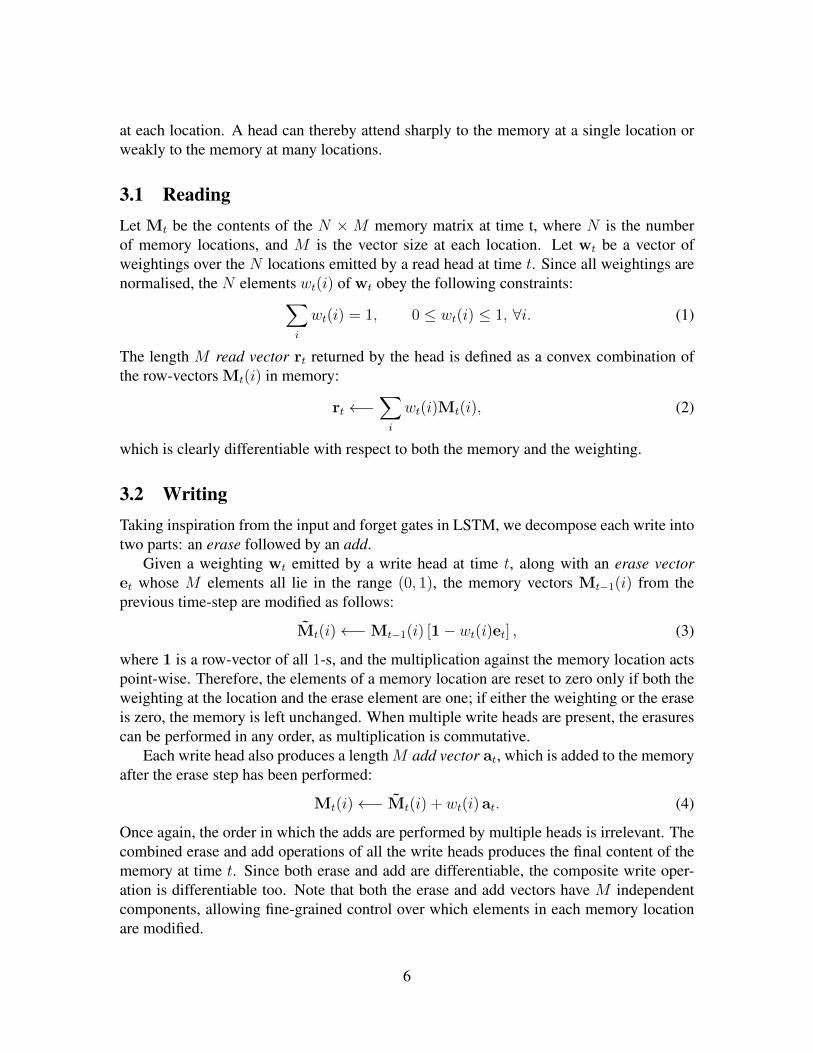
Figure 2: Flow Diagram of the Addressing Mechanism. The key vector, kt, and keystrength, βt, are used to perform content-based addressing of the memory matrix, Mt. Theresulting content-based weighting is interpolated with the weighting from the previous time stepbased on the value of the interpolation gate, gt. The shift weighting, st, determines whetherand by how much the weighting is rotated. Finally, depending on γt, the weighting is sharpenedand used for memory access.

3.3 Addressing MechanismsAlthough we have now shown the equations of reading and writing, we have not describedhow the weightings are produced. These weightings arise by combining two addressingmechanisms with complementary facilities. The first mechanism, “content-based address-ing,” focuses attention on locations based on the similarity between their current valuesand values emitted by the controller. This is related to the content-addressing of Hopfieldnetworks (Hopfield, 1982). The advantage of content-based addressing is that retrieval issimple, merely requiring the controller to produce an approximation to a part of the storeddata, which is then compared to memory to yield the exact stored value.

However, not all problems are well-suited to content-based addressing. In certain tasksthe content of a variable is arbitrary, but the variable still needs a recognisable name or ad-dress. Arithmetic problems fall into this category: the variable x and the variable y can takeon any two values, but the procedure f(x, y) = x× y should still be defined. A controllerfor this task could take the values of the variables x and y, store them in different addresses,then retrieve them and perform a multiplication algorithm. In this case, the variables areaddressed by location, not by content. We call this form of addressing “location-based ad-dressing.” Content-based addressing is strictly more general than location-based addressingas the content of a memory location could include location information inside it. In our ex-periments however, providing location-based addressing as a primitive operation provedessential for some forms of generalisation, so we employ both mechanisms concurrently.

Figure 2 presents a flow diagram of the entire addressing system that shows the orderof operations for constructing a weighting vector when reading or writing.

7

3.3.1 Focusing by Content

For content-addressing, each head (whether employed for reading or writing) first producesa length M key vector kt that is compared to each vector Mt(i) by a similarity measureK[·, ·]. The content-based system produces a normalised weighting wct based on the sim-

ilarity and a positive key strength, βt, which can amplify or attenuate the precision of thefocus:

wct (i) ←−exp

(βtK

[kt,Mt(i)

])∑

j exp

(βtK

[kt,Mt(j)

]) . (5)

In our current implementation, the similarity measure is cosine similarity:

K[u,v

]=

u · v||u|| · ||v||

. (6)

3.3.2 Focusing by Location

The location-based addressing mechanism is designed to facilitate both simple iterationacross the locations of the memory and random-access jumps. It does so by implementinga rotational shift of a weighting. For example, if the current weighting focuses entirely ona single location, a rotation of 1 would shift the focus to the next location. A negative shiftwould move the weighting in the opposite direction.

Prior to rotation, each head emits a scalar interpolation gate gt in the range (0, 1). Thevalue of g is used to blend between the weighting wt−1 produced by the head at the previoustime-step and the weighting wc

t produced by the content system at the current time-step,yielding the gated weighting wg

t :

wgt ←− gtw

ct + (1− gt)wt−1. (7)

If the gate is zero, then the content weighting is entirely ignored, and the weighting from theprevious time step is used. Conversely, if the gate is one, the weighting from the previousiteration is ignored, and the system applies content-based addressing.

After interpolation, each head emits a shift weighting st that defines a normalised distri-bution over the allowed integer shifts. For example, if shifts between -1 and 1 are allowed,st has three elements corresponding to the degree to which shifts of -1, 0 and 1 are per-formed. The simplest way to define the shift weightings is to use a softmax layer of theappropriate size attached to the controller. We also experimented with another technique,where the controller emits a single scalar that is interpreted as the lower bound of a widthone uniform distribution over shifts. For example, if the shift scalar is 6.7, then st(6) = 0.3,st(7) = 0.7, and the rest of st is zero.

8

If we index the N memory locations from 0 to N − 1, the rotation applied to wgt by st

can be expressed as the following circular convolution:

w̃t(i)←−N−1∑j=0

wgt (j) st(i− j) (8)

where all index arithmetic is computed modulo N . The convolution operation in Equa-tion (8) can cause leakage or dispersion of weightings over time if the shift weighting isnot sharp. For example, if shifts of -1, 0 and 1 are given weights of 0.1, 0.8 and 0.1, therotation will transform a weighting focused at a single point into one slightly blurred overthree points. To combat this, each head emits one further scalar γt ≥ 1 whose effect is tosharpen the final weighting as follows:

wt(i)←−w̃t(i)

γt∑j w̃t(j)

γt(9)

The combined addressing system of weighting interpolation and content and location-based addressing can operate in three complementary modes. One, a weighting can bechosen by the content system without any modification by the location system. Two, aweighting produced by the content addressing system can be chosen and then shifted. Thisallows the focus to jump to a location next to, but not on, an address accessed by content;in computational terms this allows a head to find a contiguous block of data, then access aparticular element within that block. Three, a weighting from the previous time step canbe rotated without any input from the content-based addressing system. This allows theweighting to iterate through a sequence of addresses by advancing the same distance ateach time-step.

3.4 Controller NetworkThe NTM architecture architecture described above has several free parameters, includingthe size of the memory, the number of read and write heads, and the range of allowed lo-cation shifts. But perhaps the most significant architectural choice is the type of neuralnetwork used as the controller. In particular, one has to decide whether to use a recurrentor feedforward network. A recurrent controller such as LSTM has its own internal memorythat can complement the larger memory in the matrix. If one compares the controller tothe central processing unit in a digital computer (albeit with adaptive rather than predefinedinstructions) and the memory matrix to RAM, then the hidden activations of the recurrentcontroller are akin to the registers in the processor. They allow the controller to mix infor-mation across multiple time steps of operation. On the other hand a feedforward controllercan mimic a recurrent network by reading and writing at the same location in memory atevery step. Furthermore, feedforward controllers often confer greater transparency to thenetwork’s operation because the pattern of reading from and writing to the memory matrixis usually easier to interpret than the internal state of an RNN. However, one limitation of

9

a feedforward controller is that the number of concurrent read and write heads imposes abottleneck on the type of computation the NTM can perform. With a single read head, itcan perform only a unary transform on a single memory vector at each time-step, with tworead heads it can perform binary vector transforms, and so on. Recurrent controllers caninternally store read vectors from previous time-steps, so do not suffer from this limitation.

4 ExperimentsThis section presents preliminary experiments on a set of simple algorithmic tasks suchas copying and sorting data sequences. The goal was not only to establish that NTM isable to solve the problems, but also that it is able to do so by learning compact internalprograms. The hallmark of such solutions is that they generalise well beyond the range ofthe training data. For example, we were curious to see if a network that had been trainedto copy sequences of length up to 20 could copy a sequence of length 100 with no furthertraining.

For all the experiments we compared three architectures: NTM with a feedforwardcontroller, NTM with an LSTM controller, and a standard LSTM network. Because allthe tasks were episodic, we reset the dynamic state of the networks at the start of eachinput sequence. For the LSTM networks, this meant setting the previous hidden state equalto a learned bias vector. For NTM the previous state of the controller, the value of theprevious read vectors, and the contents of the memory were all reset to bias values. Allthe tasks were supervised learning problems with binary targets; all networks had logisticsigmoid output layers and were trained with the cross-entropy objective function. Sequenceprediction errors are reported in bits-per-sequence. For more details about the experimentalparameters see Section 4.6.

4.1 CopyThe copy task tests whether NTM can store and recall a long sequence of arbitrary in-formation. The network is presented with an input sequence of random binary vectorsfollowed by a delimiter flag. Storage and access of information over long time periods hasalways been problematic for RNNs and other dynamic architectures. We were particularlyinterested to see if an NTM is able to bridge longer time delays than LSTM.

The networks were trained to copy sequences of eight bit random vectors, where thesequence lengths were randomised between 1 and 20. The target sequence was simply acopy of the input sequence (without the delimiter flag). Note that no inputs were presentedto the network while it receives the targets, to ensure that it recalls the entire sequence withno intermediate assistance.

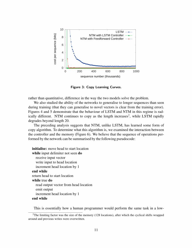
As can be seen from Figure 3, NTM (with either a feedforward or LSTM controller)learned much faster than LSTM alone, and converged to a lower cost. The disparity be-tween the NTM and LSTM learning curves is dramatic enough to suggest a qualitative,

10

0

2

4

6

8

10

0 200 400 600 800 1000

cost

per

seq

uenc

e (b

its)

sequence number (thousands)

LSTMNTM with LSTM Controller

NTM with Feedforward Controller

Figure 3: Copy Learning Curves.

rather than quantitative, difference in the way the two models solve the problem.We also studied the ability of the networks to generalise to longer sequences than seen

during training (that they can generalise to novel vectors is clear from the training error).Figures 4 and 5 demonstrate that the behaviour of LSTM and NTM in this regime is rad-ically different. NTM continues to copy as the length increases2, while LSTM rapidlydegrades beyond length 20.

The preceding analysis suggests that NTM, unlike LSTM, has learned some form ofcopy algorithm. To determine what this algorithm is, we examined the interaction betweenthe controller and the memory (Figure 6). We believe that the sequence of operations per-formed by the network can be summarised by the following pseudocode:

initialise: move head to start locationwhile input delimiter not seen do

receive input vectorwrite input to head locationincrement head location by 1

end whilereturn head to start locationwhile true do

read output vector from head locationemit outputincrement head location by 1

end while

This is essentially how a human programmer would perform the same task in a low-2The limiting factor was the size of the memory (128 locations), after which the cyclical shifts wrapped

around and previous writes were overwritten.

11

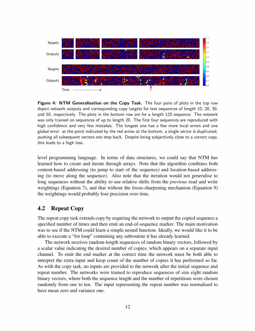
Figure 4: NTM Generalisation on the Copy Task. The four pairs of plots in the top rowdepict network outputs and corresponding copy targets for test sequences of length 10, 20, 30,and 50, respectively. The plots in the bottom row are for a length 120 sequence. The networkwas only trained on sequences of up to length 20. The first four sequences are reproduced withhigh confidence and very few mistakes. The longest one has a few more local errors and oneglobal error: at the point indicated by the red arrow at the bottom, a single vector is duplicated,pushing all subsequent vectors one step back. Despite being subjectively close to a correct copy,this leads to a high loss.

level programming language. In terms of data structures, we could say that NTM haslearned how to create and iterate through arrays. Note that the algorithm combines bothcontent-based addressing (to jump to start of the sequence) and location-based address-ing (to move along the sequence). Also note that the iteration would not generalise tolong sequences without the ability to use relative shifts from the previous read and writeweightings (Equation 7), and that without the focus-sharpening mechanism (Equation 9)the weightings would probably lose precision over time.

4.2 Repeat CopyThe repeat copy task extends copy by requiring the network to output the copied sequence aspecified number of times and then emit an end-of-sequence marker. The main motivationwas to see if the NTM could learn a simple nested function. Ideally, we would like it to beable to execute a “for loop” containing any subroutine it has already learned.

The network receives random-length sequences of random binary vectors, followed bya scalar value indicating the desired number of copies, which appears on a separate inputchannel. To emit the end marker at the correct time the network must be both able tointerpret the extra input and keep count of the number of copies it has performed so far.As with the copy task, no inputs are provided to the network after the initial sequence andrepeat number. The networks were trained to reproduce sequences of size eight randombinary vectors, where both the sequence length and the number of repetitions were chosenrandomly from one to ten. The input representing the repeat number was normalised tohave mean zero and variance one.

12

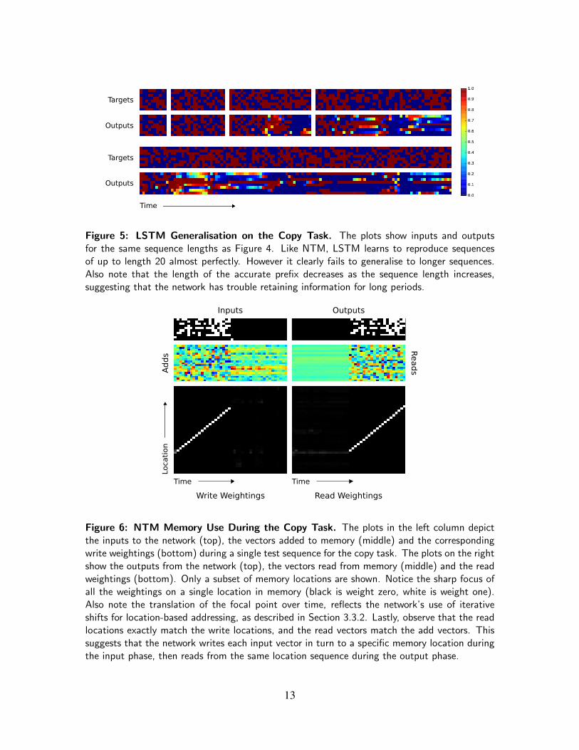
Figure 5: LSTM Generalisation on the Copy Task. The plots show inputs and outputsfor the same sequence lengths as Figure 4. Like NTM, LSTM learns to reproduce sequencesof up to length 20 almost perfectly. However it clearly fails to generalise to longer sequences.Also note that the length of the accurate prefix decreases as the sequence length increases,suggesting that the network has trouble retaining information for long periods.

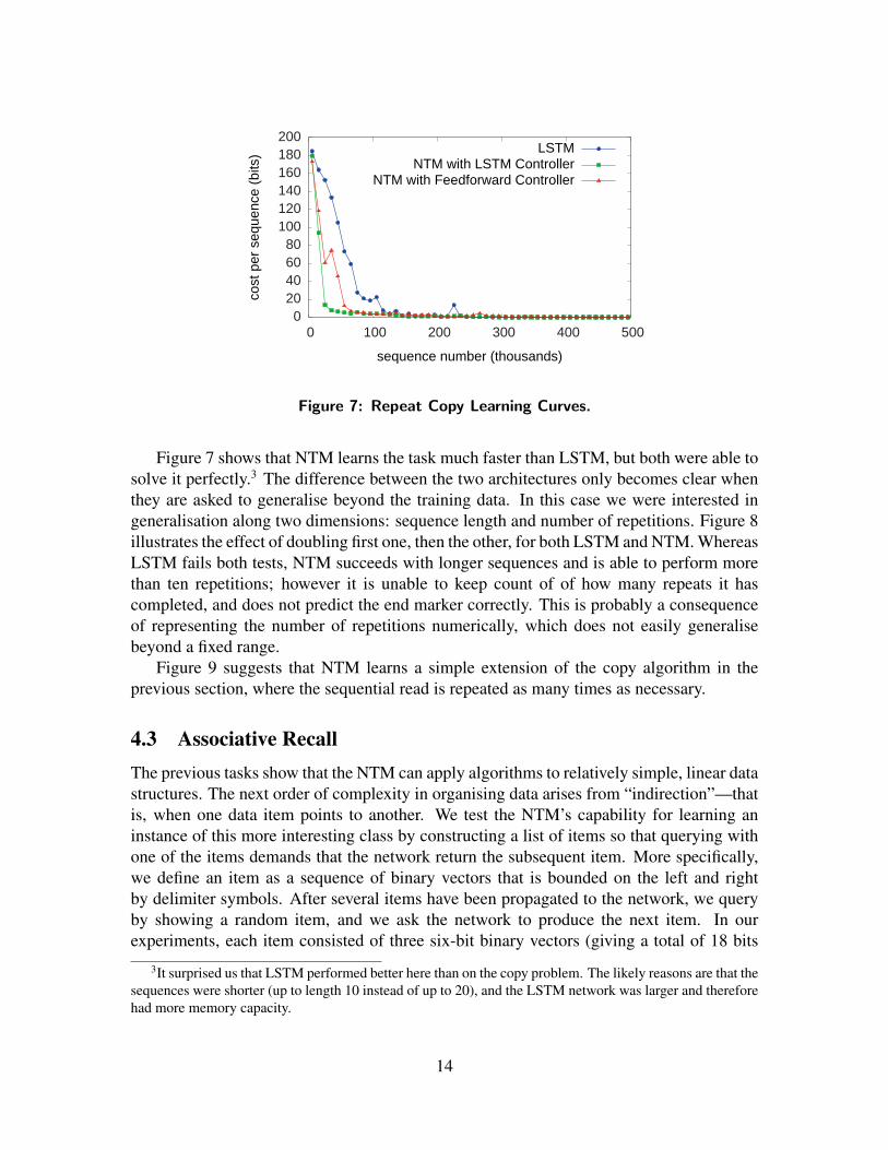
Figure 6: NTM Memory Use During the Copy Task. The plots in the left column depictthe inputs to the network (top), the vectors added to memory (middle) and the correspondingwrite weightings (bottom) during a single test sequence for the copy task. The plots on the rightshow the outputs from the network (top), the vectors read from memory (middle) and the readweightings (bottom). Only a subset of memory locations are shown. Notice the sharp focus ofall the weightings on a single location in memory (black is weight zero, white is weight one).Also note the translation of the focal point over time, reflects the network’s use of iterativeshifts for location-based addressing, as described in Section 3.3.2. Lastly, observe that the readlocations exactly match the write locations, and the read vectors match the add vectors. Thissuggests that the network writes each input vector in turn to a specific memory location duringthe input phase, then reads from the same location sequence during the output phase.

13

0 20 40 60 80

100 120 140 160 180 200

0 100 200 300 400 500

cost

per

seq

uenc

e (b

its)

sequence number (thousands)

LSTMNTM with LSTM Controller

NTM with Feedforward Controller

Figure 7: Repeat Copy Learning Curves.

Figure 7 shows that NTM learns the task much faster than LSTM, but both were able tosolve it perfectly.3 The difference between the two architectures only becomes clear whenthey are asked to generalise beyond the training data. In this case we were interested ingeneralisation along two dimensions: sequence length and number of repetitions. Figure 8illustrates the effect of doubling first one, then the other, for both LSTM and NTM. WhereasLSTM fails both tests, NTM succeeds with longer sequences and is able to perform morethan ten repetitions; however it is unable to keep count of of how many repeats it hascompleted, and does not predict the end marker correctly. This is probably a consequenceof representing the number of repetitions numerically, which does not easily generalisebeyond a fixed range.

Figure 9 suggests that NTM learns a simple extension of the copy algorithm in theprevious section, where the sequential read is repeated as many times as necessary.

4.3 Associative RecallThe previous tasks show that the NTM can apply algorithms to relatively simple, linear datastructures. The next order of complexity in organising data arises from “indirection”—thatis, when one data item points to another. We test the NTM’s capability for learning aninstance of this more interesting class by constructing a list of items so that querying withone of the items demands that the network return the subsequent item. More specifically,we define an item as a sequence of binary vectors that is bounded on the left and rightby delimiter symbols. After several items have been propagated to the network, we queryby showing a random item, and we ask the network to produce the next item. In ourexperiments, each item consisted of three six-bit binary vectors (giving a total of 18 bits

3It surprised us that LSTM performed better here than on the copy problem. The likely reasons are that thesequences were shorter (up to length 10 instead of up to 20), and the LSTM network was larger and thereforehad more memory capacity.

14

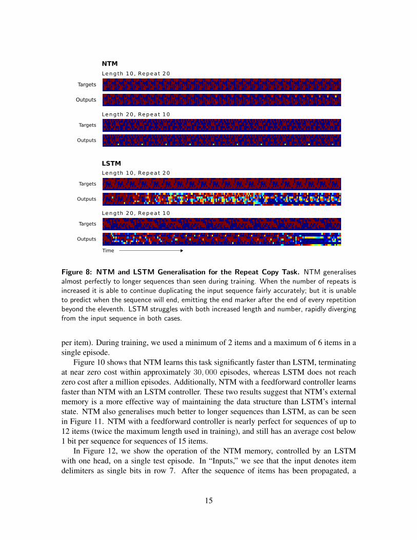
Figure 8: NTM and LSTM Generalisation for the Repeat Copy Task. NTM generalisesalmost perfectly to longer sequences than seen during training. When the number of repeats isincreased it is able to continue duplicating the input sequence fairly accurately; but it is unableto predict when the sequence will end, emitting the end marker after the end of every repetitionbeyond the eleventh. LSTM struggles with both increased length and number, rapidly divergingfrom the input sequence in both cases.

per item). During training, we used a minimum of 2 items and a maximum of 6 items in asingle episode.

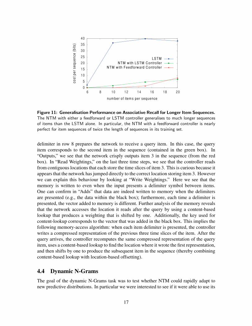
Figure 10 shows that NTM learns this task significantly faster than LSTM, terminatingat near zero cost within approximately 30, 000 episodes, whereas LSTM does not reachzero cost after a million episodes. Additionally, NTM with a feedforward controller learnsfaster than NTM with an LSTM controller. These two results suggest that NTM’s externalmemory is a more effective way of maintaining the data structure than LSTM’s internalstate. NTM also generalises much better to longer sequences than LSTM, as can be seenin Figure 11. NTM with a feedforward controller is nearly perfect for sequences of up to12 items (twice the maximum length used in training), and still has an average cost below1 bit per sequence for sequences of 15 items.

In Figure 12, we show the operation of the NTM memory, controlled by an LSTMwith one head, on a single test episode. In “Inputs,” we see that the input denotes itemdelimiters as single bits in row 7. After the sequence of items has been propagated, a

15

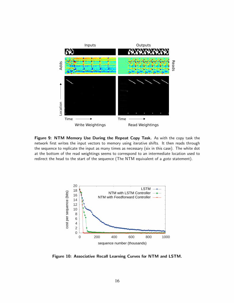
Figure 9: NTM Memory Use During the Repeat Copy Task. As with the copy task thenetwork first writes the input vectors to memory using iterative shifts. It then reads throughthe sequence to replicate the input as many times as necessary (six in this case). The white dotat the bottom of the read weightings seems to correspond to an intermediate location used toredirect the head to the start of the sequence (The NTM equivalent of a goto statement).

0 2 4 6 8

10 12 14 16 18 20

0 200 400 600 800 1000

cost

per

seq

uenc

e (b

its)

sequence number (thousands)

LSTMNTM with LSTM Controller

NTM with Feedforward Controller

Figure 10: Associative Recall Learning Curves for NTM and LSTM.

16

0

5

10

15

20

25

30

35

40

6 8 10 12 14 16 18 20

co

st

pe

r s

eq

ue

nc

e (

bit

s)

num ber o f item s per sequence

LS TMN TM w ith LS TM C ontro lle r

N TM w ith Feedforw ard C ontro lle r

Figure 11: Generalisation Performance on Associative Recall for Longer Item Sequences.The NTM with either a feedforward or LSTM controller generalises to much longer sequencesof items than the LSTM alone. In particular, the NTM with a feedforward controller is nearlyperfect for item sequences of twice the length of sequences in its training set.

delimiter in row 8 prepares the network to receive a query item. In this case, the queryitem corresponds to the second item in the sequence (contained in the green box). In“Outputs,” we see that the network crisply outputs item 3 in the sequence (from the redbox). In “Read Weightings,” on the last three time steps, we see that the controller readsfrom contiguous locations that each store the time slices of item 3. This is curious because itappears that the network has jumped directly to the correct location storing item 3. Howeverwe can explain this behaviour by looking at “Write Weightings.” Here we see that thememory is written to even when the input presents a delimiter symbol between items.One can confirm in “Adds” that data are indeed written to memory when the delimitersare presented (e.g., the data within the black box); furthermore, each time a delimiter ispresented, the vector added to memory is different. Further analysis of the memory revealsthat the network accesses the location it reads after the query by using a content-basedlookup that produces a weighting that is shifted by one. Additionally, the key used forcontent-lookup corresponds to the vector that was added in the black box. This implies thefollowing memory-access algorithm: when each item delimiter is presented, the controllerwrites a compressed representation of the previous three time slices of the item. After thequery arrives, the controller recomputes the same compressed representation of the queryitem, uses a content-based lookup to find the location where it wrote the first representation,and then shifts by one to produce the subsequent item in the sequence (thereby combiningcontent-based lookup with location-based offsetting).

4.4 Dynamic N-GramsThe goal of the dynamic N-Grams task was to test whether NTM could rapidly adapt tonew predictive distributions. In particular we were interested to see if it were able to use its

17

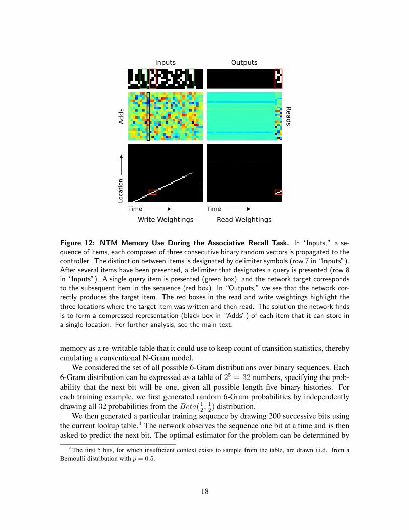
Figure 12: NTM Memory Use During the Associative Recall Task. In “Inputs,” a se-quence of items, each composed of three consecutive binary random vectors is propagated to thecontroller. The distinction between items is designated by delimiter symbols (row 7 in “Inputs”).After several items have been presented, a delimiter that designates a query is presented (row 8in “Inputs”). A single query item is presented (green box), and the network target correspondsto the subsequent item in the sequence (red box). In “Outputs,” we see that the network cor-rectly produces the target item. The red boxes in the read and write weightings highlight thethree locations where the target item was written and then read. The solution the network findsis to form a compressed representation (black box in “Adds”) of each item that it can store ina single location. For further analysis, see the main text.

memory as a re-writable table that it could use to keep count of transition statistics, therebyemulating a conventional N-Gram model.

We considered the set of all possible 6-Gram distributions over binary sequences. Each6-Gram distribution can be expressed as a table of 25 = 32 numbers, specifying the prob-ability that the next bit will be one, given all possible length five binary histories. Foreach training example, we first generated random 6-Gram probabilities by independentlydrawing all 32 probabilities from the Beta(1

2, 12) distribution.

We then generated a particular training sequence by drawing 200 successive bits usingthe current lookup table.4 The network observes the sequence one bit at a time and is thenasked to predict the next bit. The optimal estimator for the problem can be determined by

4The first 5 bits, for which insufficient context exists to sample from the table, are drawn i.i.d. from aBernoulli distribution with p = 0.5.

18

130

135

140

145

150

155

160

0 200 400 600 800 1000

cost

per

seq

uenc

e (b

its)

sequence number (thousands)

LSTMNTM with LSTM Controller

NTM with Feedforward ControllerOptimal Estimator

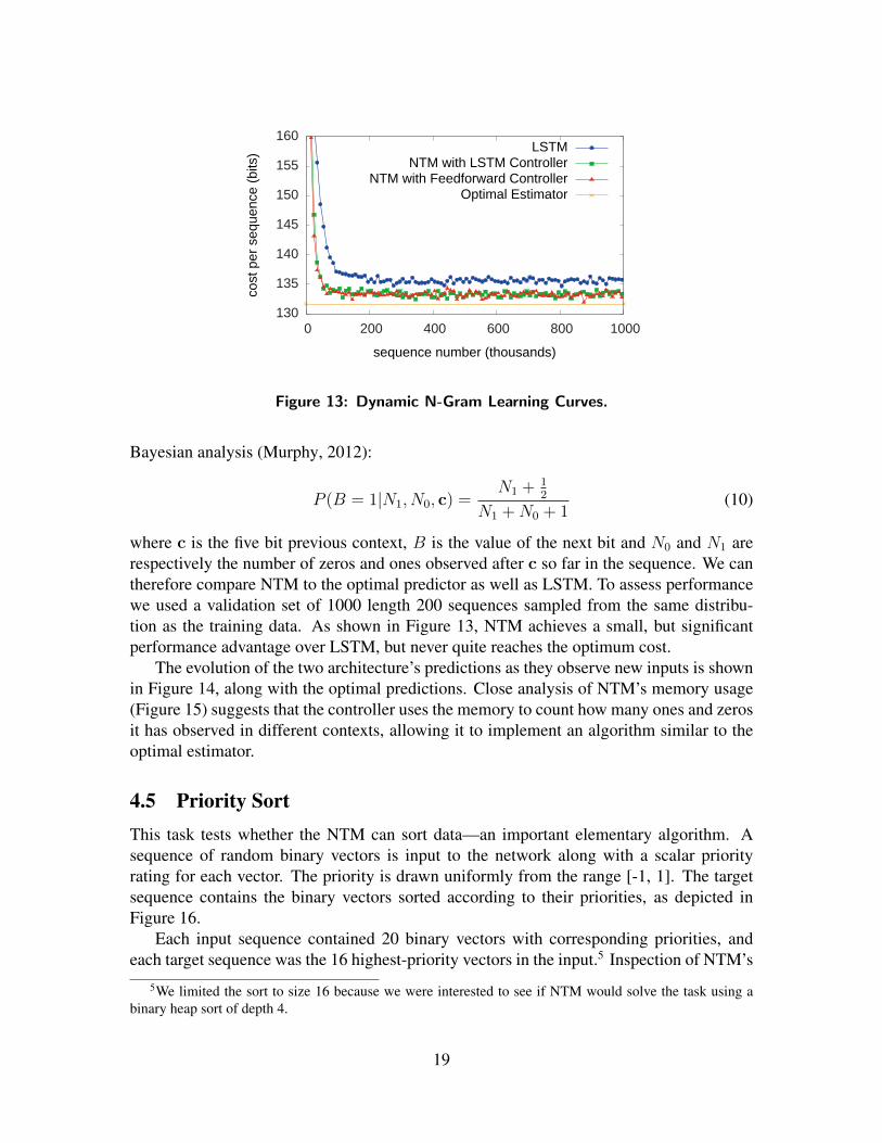
Figure 13: Dynamic N-Gram Learning Curves.

Bayesian analysis (Murphy, 2012):

P (B = 1|N1, N0, c) =N1 +

12

N1 +N0 + 1(10)

where c is the five bit previous context, B is the value of the next bit and N0 and N1 arerespectively the number of zeros and ones observed after c so far in the sequence. We cantherefore compare NTM to the optimal predictor as well as LSTM. To assess performancewe used a validation set of 1000 length 200 sequences sampled from the same distribu-tion as the training data. As shown in Figure 13, NTM achieves a small, but significantperformance advantage over LSTM, but never quite reaches the optimum cost.

The evolution of the two architecture’s predictions as they observe new inputs is shownin Figure 14, along with the optimal predictions. Close analysis of NTM’s memory usage(Figure 15) suggests that the controller uses the memory to count how many ones and zerosit has observed in different contexts, allowing it to implement an algorithm similar to theoptimal estimator.

4.5 Priority SortThis task tests whether the NTM can sort data—an important elementary algorithm. Asequence of random binary vectors is input to the network along with a scalar priorityrating for each vector. The priority is drawn uniformly from the range [-1, 1]. The targetsequence contains the binary vectors sorted according to their priorities, as depicted inFigure 16.

Each input sequence contained 20 binary vectors with corresponding priorities, andeach target sequence was the 16 highest-priority vectors in the input.5 Inspection of NTM’s

5We limited the sort to size 16 because we were interested to see if NTM would solve the task using abinary heap sort of depth 4.

19

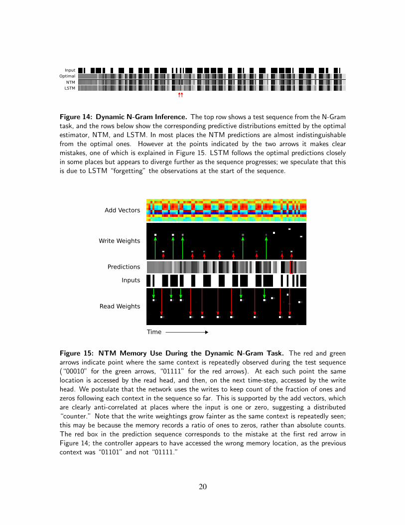
Figure 14: Dynamic N-Gram Inference. The top row shows a test sequence from the N-Gramtask, and the rows below show the corresponding predictive distributions emitted by the optimalestimator, NTM, and LSTM. In most places the NTM predictions are almost indistinguishablefrom the optimal ones. However at the points indicated by the two arrows it makes clearmistakes, one of which is explained in Figure 15. LSTM follows the optimal predictions closelyin some places but appears to diverge further as the sequence progresses; we speculate that thisis due to LSTM “forgetting” the observations at the start of the sequence.

Figure 15: NTM Memory Use During the Dynamic N-Gram Task. The red and greenarrows indicate point where the same context is repeatedly observed during the test sequence(“00010” for the green arrows, “01111” for the red arrows). At each such point the samelocation is accessed by the read head, and then, on the next time-step, accessed by the writehead. We postulate that the network uses the writes to keep count of the fraction of ones andzeros following each context in the sequence so far. This is supported by the add vectors, whichare clearly anti-correlated at places where the input is one or zero, suggesting a distributed“counter.” Note that the write weightings grow fainter as the same context is repeatedly seen;this may be because the memory records a ratio of ones to zeros, rather than absolute counts.The red box in the prediction sequence corresponds to the mistake at the first red arrow inFigure 14; the controller appears to have accessed the wrong memory location, as the previouscontext was “01101” and not “01111.”

20

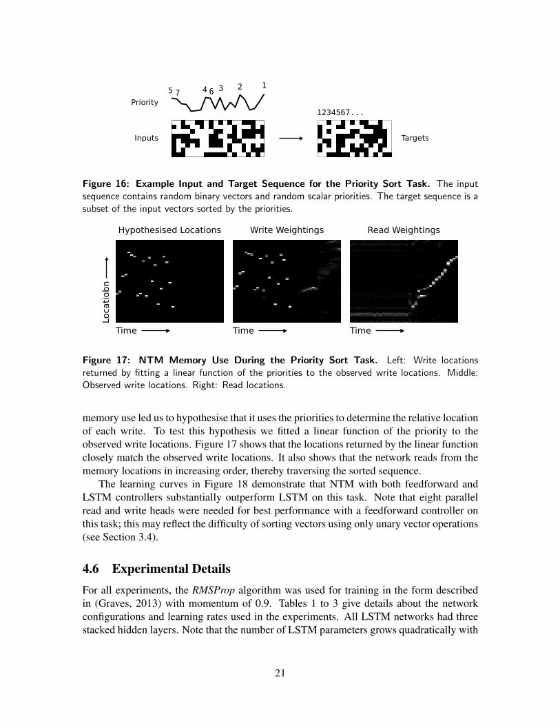
Figure 16: Example Input and Target Sequence for the Priority Sort Task. The inputsequence contains random binary vectors and random scalar priorities. The target sequence is asubset of the input vectors sorted by the priorities.

Write Weightings Read WeightingsHypothesised Locations

Time Time Time

Loca

tiobn

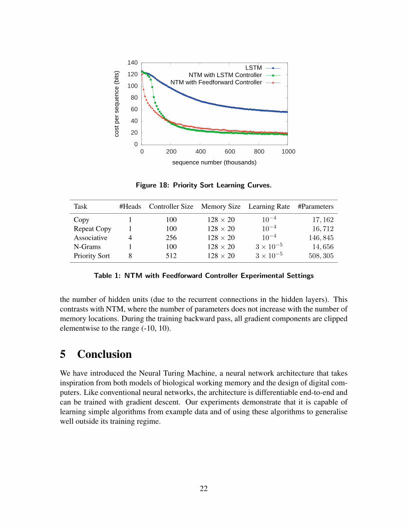
Figure 17: NTM Memory Use During the Priority Sort Task. Left: Write locationsreturned by fitting a linear function of the priorities to the observed write locations. Middle:Observed write locations. Right: Read locations.

memory use led us to hypothesise that it uses the priorities to determine the relative locationof each write. To test this hypothesis we fitted a linear function of the priority to theobserved write locations. Figure 17 shows that the locations returned by the linear functionclosely match the observed write locations. It also shows that the network reads from thememory locations in increasing order, thereby traversing the sorted sequence.

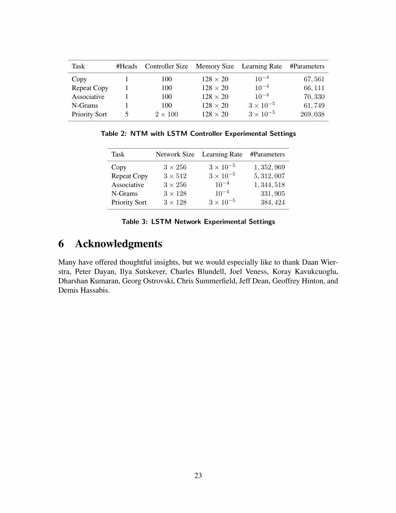
The learning curves in Figure 18 demonstrate that NTM with both feedforward andLSTM controllers substantially outperform LSTM on this task. Note that eight parallelread and write heads were needed for best performance with a feedforward controller onthis task; this may reflect the difficulty of sorting vectors using only unary vector operations(see Section 3.4).

4.6 Experimental DetailsFor all experiments, the RMSProp algorithm was used for training in the form describedin (Graves, 2013) with momentum of 0.9. Tables 1 to 3 give details about the networkconfigurations and learning rates used in the experiments. All LSTM networks had threestacked hidden layers. Note that the number of LSTM parameters grows quadratically with

21

0

20

40

60

80

100

120

140

0 200 400 600 800 1000

cost

per

seq

uenc

e (b

its)

sequence number (thousands)

LSTMNTM with LSTM Controller

NTM with Feedforward Controller

Figure 18: Priority Sort Learning Curves.

Task #Heads Controller Size Memory Size Learning Rate #Parameters

Copy 1 100 128 × 20 10−4 17, 162Repeat Copy 1 100 128 × 20 10−4 16, 712Associative 4 256 128 × 20 10−4 146, 845N-Grams 1 100 128 × 20 3× 10−5 14, 656Priority Sort 8 512 128 × 20 3× 10−5 508, 305

Table 1: NTM with Feedforward Controller Experimental Settings

the number of hidden units (due to the recurrent connections in the hidden layers). Thiscontrasts with NTM, where the number of parameters does not increase with the number ofmemory locations. During the training backward pass, all gradient components are clippedelementwise to the range (-10, 10).

5 ConclusionWe have introduced the Neural Turing Machine, a neural network architecture that takesinspiration from both models of biological working memory and the design of digital com-puters. Like conventional neural networks, the architecture is differentiable end-to-end andcan be trained with gradient descent. Our experiments demonstrate that it is capable oflearning simple algorithms from example data and of using these algorithms to generalisewell outside its training regime.

22

Task #Heads Controller Size Memory Size Learning Rate #Parameters

Copy 1 100 128 × 20 10−4 67, 561Repeat Copy 1 100 128 × 20 10−4 66, 111Associative 1 100 128 × 20 10−4 70, 330N-Grams 1 100 128 × 20 3× 10−5 61, 749Priority Sort 5 2× 100 128 × 20 3× 10−5 269, 038

Table 2: NTM with LSTM Controller Experimental Settings

Task Network Size Learning Rate #Parameters

Copy 3× 256 3× 10−5 1, 352, 969Repeat Copy 3× 512 3× 10−5 5, 312, 007Associative 3× 256 10−4 1, 344, 518N-Grams 3× 128 10−4 331, 905Priority Sort 3× 128 3× 10−5 384, 424

Table 3: LSTM Network Experimental Settings

6 AcknowledgmentsMany have offered thoughtful insights, but we would especially like to thank Daan Wier-stra, Peter Dayan, Ilya Sutskever, Charles Blundell, Joel Veness, Koray Kavukcuoglu,Dharshan Kumaran, Georg Ostrovski, Chris Summerfield, Jeff Dean, Geoffrey Hinton, andDemis Hassabis.

23

ReferencesBaddeley, A., Eysenck, M., and Anderson, M. (2009). Memory. Psychology Press.

Bahdanau, D., Cho, K., and Bengio, Y. (2014). Neural machine translation by jointlylearning to align and translate. abs/1409.0473.

Barrouillet, P., Bernardin, S., and Camos, V. (2004). Time constraints and resource shar-ing in adults’ working memory spans. Journal of Experimental Psychology: General,133(1):83.

Chomsky, N. (1956). Three models for the description of language. Information Theory,IEEE Transactions on, 2(3):113–124.

Das, S., Giles, C. L., and Sun, G.-Z. (1992). Learning context-free grammars: Capabil-ities and limitations of a recurrent neural network with an external stack memory. InProceedings of The Fourteenth Annual Conference of Cognitive Science Society. IndianaUniversity.

Dayan, P. (2008). Simple substrates for complex cognition. Frontiers in neuroscience,2(2):255.

Eliasmith, C. (2013). How to build a brain: A neural architecture for biological cognition.Oxford University Press.

Fitch, W., Hauser, M. D., and Chomsky, N. (2005). The evolution of the language faculty:clarifications and implications. Cognition, 97(2):179–210.

Fodor, J. A. and Pylyshyn, Z. W. (1988). Connectionism and cognitive architecture: Acritical analysis. Cognition, 28(1):3–71.

Frasconi, P., Gori, M., and Sperduti, A. (1998). A general framework for adaptive process-ing of data structures. Neural Networks, IEEE Transactions on, 9(5):768–786.

Gallistel, C. R. and King, A. P. (2009). Memory and the computational brain: Why cogni-tive science will transform neuroscience, volume 3. John Wiley & Sons.

Goldman-Rakic, P. S. (1995). Cellular basis of working memory. Neuron, 14(3):477–485.

Graves, A. (2013). Generating sequences with recurrent neural networks. arXiv preprintarXiv:1308.0850.

Graves, A. and Jaitly, N. (2014). Towards end-to-end speech recognition with recurrentneural networks. In Proceedings of the 31st International Conference on Machine Learn-ing (ICML-14), pages 1764–1772.

24

Graves, A., Mohamed, A., and Hinton, G. (2013). Speech recognition with deep recurrentneural networks. In Acoustics, Speech and Signal Processing (ICASSP), 2013 IEEEInternational Conference on, pages 6645–6649. IEEE.

Hadley, R. F. (2009). The problem of rapid variable creation. Neural computation,21(2):510–532.

Hazy, T. E., Frank, M. J., and O’Reilly, R. C. (2006). Banishing the homunculus: makingworking memory work. Neuroscience, 139(1):105–118.

Hinton, G. E. (1986). Learning distributed representations of concepts. In Proceedingsof the eighth annual conference of the cognitive science society, volume 1, page 12.Amherst, MA.

Hochreiter, S., Bengio, Y., Frasconi, P., and Schmidhuber, J. (2001a). Gradient flow inrecurrent nets: the difficulty of learning long-term dependencies.

Hochreiter, S. and Schmidhuber, J. (1997). Long short-term memory. Neural computation,9(8):1735–1780.

Hochreiter, S., Younger, A. S., and Conwell, P. R. (2001b). Learning to learn using gradientdescent. In Artificial Neural Networks?ICANN 2001, pages 87–94. Springer.

Hopfield, J. J. (1982). Neural networks and physical systems with emergent collectivecomputational abilities. Proceedings of the national academy of sciences, 79(8):2554–2558.

Jackendoff, R. and Pinker, S. (2005). The nature of the language faculty and its implicationsfor evolution of language (reply to fitch, hauser, and chomsky). Cognition, 97(2):211–225.

Kanerva, P. (2009). Hyperdimensional computing: An introduction to computing in dis-tributed representation with high-dimensional random vectors. Cognitive Computation,1(2):139–159.

Marcus, G. F. (2003). The algebraic mind: Integrating connectionism and cognitive sci-ence. MIT press.

Miller, G. A. (1956). The magical number seven, plus or minus two: some limits on ourcapacity for processing information. Psychological review, 63(2):81.

Miller, G. A. (2003). The cognitive revolution: a historical perspective. Trends in cognitivesciences, 7(3):141–144.

Minsky, M. L. (1967). Computation: finite and infinite machines. Prentice-Hall, Inc.

Murphy, K. P. (2012). Machine learning: a probabilistic perspective. MIT press.

25

Plate, T. A. (2003). Holographic Reduced Representation: Distributed representation forcognitive structures. CSLI.

Pollack, J. B. (1990). Recursive distributed representations. Artificial Intelligence,46(1):77–105.

Rigotti, M., Barak, O., Warden, M. R., Wang, X.-J., Daw, N. D., Miller, E. K., and Fusi,S. (2013). The importance of mixed selectivity in complex cognitive tasks. Nature,497(7451):585–590.

Rumelhart, D. E., McClelland, J. L., Group, P. R., et al. (1986). Parallel distributed pro-cessing, volume 1. MIT press.

Seung, H. S. (1998). Continuous attractors and oculomotor control. Neural Networks,11(7):1253–1258.

Siegelmann, H. T. and Sontag, E. D. (1995). On the computational power of neural nets.Journal of computer and system sciences, 50(1):132–150.

Smolensky, P. (1990). Tensor product variable binding and the representation of symbolicstructures in connectionist systems. Artificial intelligence, 46(1):159–216.

Socher, R., Huval, B., Manning, C. D., and Ng, A. Y. (2012). Semantic compositionalitythrough recursive matrix-vector spaces. In Proceedings of the 2012 Joint Conference onEmpirical Methods in Natural Language Processing and Computational Natural Lan-guage Learning, pages 1201–1211. Association for Computational Linguistics.

Sutskever, I., Martens, J., and Hinton, G. E. (2011). Generating text with recurrent neuralnetworks. In Proceedings of the 28th International Conference on Machine Learning(ICML-11), pages 1017–1024.

Sutskever, I., Vinyals, O., and Le, Q. V. (2014). Sequence to sequence learning with neuralnetworks. arXiv preprint arXiv:1409.3215.

Touretzky, D. S. (1990). Boltzcons: Dynamic symbol structures in a connectionist network.Artificial Intelligence, 46(1):5–46.

Von Neumann, J. (1945). First draft of a report on the edvac.

Wang, X.-J. (1999). Synaptic basis of cortical persistent activity: the importance of nmdareceptors to working memory. The Journal of Neuroscience, 19(21):9587–9603.

26