what resolution of mm5 is optimal for weather forecasting
TRANSCRIPT

EARTH SCIENCES CENTRE GÖTEBORG UNIVERSITY B450 2005
WHAT RESOLUTION OF MM5 IS OPTIMAL FOR WEATHER FORECASTING IN
GÖTEBORG?
Magnus Nilsson
Department of Physical Geography GÖTEBORG 2005

GÖTEBORGS UNIVERSITET Institutionen för geovetenskaper Naturgeografi Geovetarcentrum
WHAT RESOLUTION OF MM5 IS OPTIMAL FOR WEATHER FORECASTING IN
GÖTEBORG?
Magnus Nilsson
ISSN 1400-3821 B450
Projektarbete Göteborg 2005
Postadress Besöksadress Telefo Telfax Earth Sciences Centre Geovetarcentrum Geovetarcentrum 031-773 19 51 031-773 19 86 Göteborg University S-405 30 Göteborg Guldhedsgatan 5A S-405 30 Göteborg
SWEDEN


2
Abstract The main aim of this project is to set up a meteorological model, MM5 under MeteOS 2002 for the Göteborg area and to apply the model for weather forecasts. The focus is on model domain size, resolution and model performance. For this purpose temperature and sea level pressure will be examined using measurement and simulated results from different model setups. It was found that the root mean square error (RMSE) of temperature and sea level pressure decreases with increasing domain size. However, this trend was not always consistent, as in some cases, no trend was found. When quick changes of the weather occur, the model had trouble making good forecasts, which caused it to render data showing decreasing quality with increasing domain size. Most of these events were associated with relatively high RMSEs. Some of this applies to the model resolution as well. During stable conditions, increasing the resolution (15, 11 and 6 km) will in some cases enable the model to improve the quality of the output. When sudden changes occur, such as short but large temperature drops during the night, this will cause the output to severely deteriorate and if this coincides with tests of the higher resolution tests, the trend will be decreasing quality with increasing model resolution.

3
Sammanfattning Syftet med projektet är att sätta upp och konfigurera en meteorologisk modell, MM5 med hjälp av MeteOS 2002 för Göteborgsregionen samt att tillämpa modellen för väderprognoser. Fokus ligger på modellens storlek, upplösning samt kapacitet. För att undersöka detta används temperatur och lufttryck, där modellprognoser kommer att jämföras med insamlad mätdata för olika modellinställningar. Root mean square error (RMSE) för temperatur och lufttryck avtog med tilltagande modellstorlek, men trenden var inte tydlig för alla försök. Vid snabba förändringar av temperatur och lufttryck hade modellen svårigheter med att skapa tillförlitliga prognoser, vilket försvårade tolkningen av eventuella trender. Liknande resultat återfanns även i försöken med modellens upplösning. Vid stabila förhållanden kan en högre upplösning (15, 11 och 6 km) förbättra modellens prognos. Vid hastiga omslag, till exempel tillfälliga nedgångar i temperaturen under natten, sjunker prognosens kvalitet.

4
Acknowledgements The author would like to thank Professor Deliang Chen, Göteborg University, for supervising and providing financial aid during this project. Angelo Dimitrov, developer of MeteOS 2002, has been of great help with his excellent technical support while installing and running MeteOS 2002. I would also like to thank Marcus Flarup at SMHI and Jesper Lindgren at Luftnet, Miljöförvaltningen Göteborg, for providing data relevant to model output evaluation.

5
Table of contents
1 Introduction 7 1.1 Benefits of weather prediction 7 1.2 Weather prediction history 7 1.3 Meteorological models 8 1.4 Related research 8 1.5 Weather prediction in Sweden and Norway 9 1.5.1 Introduction 9 1.5.2 HIRLAM 9 1.5.3 SMHI 9 1.5.4 DNMI 11 1.5.5 Comparison of SMHI and DNMI 12
2 Objectives and scientific questions 14 2.1 Objectives 14 2.2 Scientific Questions 14
3 Study area 15 3.1 Topography and landforms 15 3.2 Climate 15
4 Data and methods 17 4.1 MeteOS 2002 and MM5 17 4.1.1 MM5 17 4.1.2 MeteOS 2002 17 4.1.3 MeteOS 2002 configuration 18 4.1.4 Choosing model domain 18 4.1.5 Choosing model resolution 19 4.1.6 Data collection stations 20 4.1.7 Test period and data 21 4.1.8 Evaluation of prediction 21
5 Results 22 5.1 Impacts of domain size 22 5.1.1 300 x 300 km 22 5.1.2 500 x 500 km 25 5.1.3 800 x 800 km 27 5.2 Effect of model resolution 30 5.2.1 15 km 30 5.2.2 11 km 32 5.2.3 6 km 32 5.3 Evaluation of statistical analysis 34 5.3.1 Säve 34 5.3.2 Skanstorget 35 5.3.3 Nidingen 35

6
6 Discussion 37 6.1 Impact of domain size 37 6.1.1 Temperature 37 6.1.2 Sea level pressure 37 6.2 Effect of model resolution 37 6.2.1 Temperature 37 6.2.2 Sea level pressure 38 6.3 Uncertainties 38 6.3.1 Modelling problems 38 6.3.2 SMHI / Luftnet data 38
7 Conclusions 40
References

7
1 Introduction 1.1 Benefits of weather prediction There are several sectors that would benefit from higher quality of the weather predictions. Graham et al. list a few of them. Agriculture is one example where additional accuracy could help prepare for temperatures below zero, i.e. situations where freeze prevention methods can be deployed. Hurricane tracks are another case where improved predictions might help, for example when it comes to evacuation of exposed communities. Graham et al. also mention that military operations and the aviation industry could benefit from improved weather predictions. Most parts of the society will benefit from high quality predictions.
1.2 Weather prediction history During the 19th century, the capabilities for collecting and distributing meteorological data were radically improved due to inventions such as the telegraph. This enabled rapid collection of data from a wide range of sources and the production of basic weather maps. The capacity was further advanced in the 1920s by the introduction of the radiosonde, which allowed data collection from high altitudes, up to 30 km (Graham et al.). One of the first steps towards weather prediction, and not just data collection, was taken by Vilhelm Bjerknes, a Norwegian mathematician (Graham et al.). Early in the 20th century, he founded the Bergen Geophysical institute where he concluded that by solving mathematical equations, the weather could be predicted. However, the equations were too complex for any practical use in weather predictions. The next step was taken by Lewis Fry Richardson, a Scotch mathematician. He reduced the complex equations made by Bjerknes and published them in his book, Weather Prediction by Numerical Process, in 1922. Richardson extrapolated the computed meteorological information and used the new data to extrapolate even further in time. Still, though, the equations were too complex to solve by hand for any large scale tests. A simple attempt was made with surface pressure tendencies at two grid points, but the results were unsatisfactory. Low quality of the initial data was blamed for the poor results but it was later found that Richardson´s equations were associated with significant miscalculations (Holton 2002). The Development of numerical meteorological models was close to non-existent until the years after World War II, when a growing number of meteorological observation stations made high quality data available to the models (Holton 2002). The introduction of computers enabled scientists to handle the massive calculations involved in numerical weather predictions. In 1948, Jule Charney, a meteorological theoretician, was able to forecast general wind patterns, using simplified models of the atmosphere (European Centre for Medium-Range Weather Forecasts (hereafter ECMWF), 2002). It was found that Richardson´s equations, left unchanged, within a few time steps would generate ”noise” that would drown the real trend. The fact that a initial small inaccuracy can disturb the calculations has been discussed by Edward Lorenz (1988), who names it computational chaos, the "... rapid and unbounded amplification of the variables...". Experiments in 1950, using the most simple of Charney´s equations, the barotropic model of motion in the atmosphere, were able to predict patterns over North America for the next 24 hours with greater accuracy than before. Some countries, those with small computational power, focused on models using the barotropic state, while other, more resourceful, countries used baroclinic numerical models. Due to the complexity of the calculations, barotropic models were the most common ones in the 1950s, while the baroclinic emerged in the 1960s (ECMWF 2002). When models based on primitive equations (PE-models) were introduced, it meant greater accuracy that previous models as PE-models allowed features such as convection to be simulated. This is crucial to many regions, for example the tropics. In 1966, the first global PE-model was initiated at

8
NMC Washington with a 300 km grid resolution and a vertical resolution of six layers. During the next decade, several PE-models with various resolutions and sizes were used (ECMWF 2002). Weather prediction has benefited considerably from technological development, such as computers, satellites and data from high altitude and distant locations (Graham et al.). One example is the European Eurosat 1 satellite, launched in 1977 by the European Space Agency. One of the aims of this project was to collect data for cloud cover. Meteosat 1 has been followed by other meteorological satellites and the project now distributes satellite images every 30 minutes. The grid resolution has increased during the last decades. It can generally be concluded that while the earliest models focused on large scale global dynamics, recent model development has enabled scientists to study meteorological features on a regional and local scale.
1.3 Meteorological models Currently, there are a number of models used for weather prediction. Here, it is important to separate global models from mesoscale models. Table 1 shows a few examples of models.
Table 1. Weather prediction models (Dimitrov 2002).
Global Models Mesoscale Models
AVN / GFS, National Centers for Environmental Predictions
ARPS, University of Oklahoma
ECMWF, European Centre for Medium-Range Weather
Forecasts
HIRLAM, European Centre for Medium-Range Weather
Forecasts
GSM, National Centers for Environmental Predictions
MM5, University Corporation for Atmsospheric
Research
MRF, NOAA
RAMS, Colorado State University
NOGAPS, U.S. Navy
RUC, National Oceanic and Atmospheric
Administration
Generally, the resolution of the global models is coarse due to the massive volume of data involved. In this paper, one of the mesoscale models, the MM5, has been used. It is integrated with the MeteOS, a Linux software package for creating weather predictions. MM5 is a widely recognitioned model, used by for example IBM, University of Washington and NOAA. MeteOS is developed by Storm laboratory in Bulgaria. MeteOS and MM5 are further discussed in 4.1.
1.4 Related research The significance of model resolution and domain size are not matters where much research has been performed, specially when it comes to weather forecasts. Booij (2004) has studied the significance of different spatial resolutions to climate change and river flooding. When comparing the average and extreme discharge behavior, it was found that "...the results become somewhat better with increasing model resolution...".

9
Horritt & Bates (2001) have compared a set of resolutions, ranging from 1000 to 10 m, when modeling flood flow. Their conclusion was that "...the model reaching maximum performance at a resolution of 100 m, after which no improvement is seen with increasing resolution". Information from these projects might help when assessing the results in this paper.
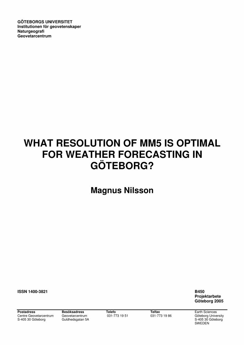
1.5 Weather prediction in Sweden and Norway 1.5.1 Introduction All of the Nordic countries use computer models for predicting the atmospheric motion and the weather. However, since the optimal model setup is unknown, each country uses a different set of model parameters for weather forecasts. Since the objectives of this paper are to examine the effect of some model properties, it is of interest to consider the setups that some countries have chosen. The approach of Sweden and Norway has been studied in this paper. 1.5.2 HIRLAM HIRLAM, High Resolution Limited Area Model, is the model used in Denmark, Finland, Iceland, Ireland, Netherlands, Norway, Spain and Sweden. The project was started in 1985 and the main objective is to "...provide an operational production system for short-range forecasting which generates a comprehensive set of Numerical Weather Prediction (NWP) products of highest quality" (Undén 2002). It is maintained at ECMWF in what is called the Reference System, which is updated a few times a year. Here, various tools for data collection, modeling, post processing, diagnostics and verification can be found (HIRLAM management team). One important aspect of modeling is the parameterization at different resolutions. Since "...resolution defines an ability to resolve a given phenomenon..." (Undén 2002), it is important to choose an appropriate model resolution and be aware of the consequences. One example is the slope of the ground, which will have influence on radiation as the resolution increases. The significance of this issue will increase as the model resolution increases to some 10 km, and the grid size decreases, and is not dealt with in the current HIRLAM version. Undén (2002) also exemplifies the problems associated with parameterization with processes such as convection, i.e. heat and moisture transport. Pielke (2002) states that “...the accuracy of any one parameterization in a model need not be any more precise than the least accurate parameterization of significant physical processes for the atmospheric system of interest”. This demonstrates the importance of single variables and the effect of miscalculations. HIRLAM collects data on lower boundary conditions from databases such as Global 30 Arc Second Elevation data (GTOPO30), 1998, and Global Land Cover Charactesistics (GLCC), 1997, constructed by U.S. Geological Survey. Five catogories of surface characteristics are used in HIRLAM: forest, low vegetation, bare ground, sea/lake and ice. This, too, has effects on the physical parameterization (Undén 2002). In addition to these, there are a number of other data sources. Included here are data for surface temperature, soil moisture, soil properties and other sources. Figure 1 shows the type of data used in the model.
10
Figure 1. The various data sources in HIRLAM (Undén 2002).
For verification purposes, HIRLAM includes methods for analyzing the data. This is done for several reasons. For example, the model might perform unsatisfactorily under some specific meteorological conditions, which requires long term studies. Also, it is important to evaluate the results when changes in the model architecture are introduced. Undén (2002) states that “...new releases of the Hirlam NWP system have to be compared to the current reference version over a collection of periods containing all relevant weather conditions”. If the results are improved under some conditions and deteriorated under others, the changes have to be evaluated. Undén (2002) writes that “...the choice for a new model version is in part a value statement...”. The European Centre for Medium-Range Weather Forecasts, ECMWF, was founded in 1973 and its task was to coordinate some of the meteoroligical efforts of its associates (DNMI 2001). ECMWF provides the HIRLAM member states with boundary values four times a day. This data is thereafter used in the nested models with a resolution two to five times higher than that of ECMWF, which has the resolution of 0.5 x 0.5° with 31 vertical levels (Undén 2002). 1.5.3 SMHI In Sweden, SMHI, The Swedish Meteorological and Hydrological Institute, is the organization that handles issues related to meteorology, hydrology and oceanography. It is also responsible for the national HIRLAM modeling and development since 1982. In SMHI, HIRLAM related work is partly managed by The Rossby Centre, a section of SWECLIM, the Swedish regional climate modeling program. The national version of HIRLAM is called the Rossby Centre Regional Climate Model, RCA, and the first version was introduced in 1998 (Undén 2002). For weather prediction, SMHI uses HIRLAM with two different domain sizes. Figure 2 shows the different spatial resolutions in the Swedish setup of HIRLAM.
11
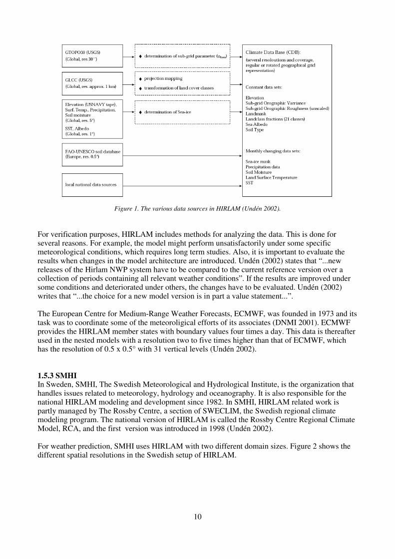
Figure 2. SMHI HIRLAM domain sizes (Meuller 2003).
The outer box features a resolution of 44 km while the resolution in the center is 22 km. Boundary data are transferred from the outer to the inner box. Both areas have 40 vertical layers. Meuller (2004) states that these resolutions are quite low and that the model resolution the summer of 2004 will change to 22 km for the outer box and 11 km for the inner box, now featuring 60 vertical layers. The long term ambition is to produce a weather prediction system with horisontal resolutions below 10 km (Andræ 2001). SMHI has an operational schedule of HIRLAM, where the model is run with the coarse grid, called H44, out to 48 hours where the model shifts to the finer resolution, H22. The initial data is collected from ECMWF. SMHI uses version 5.1.4 of HIRLAM. 1.5.4 DNMI DNMI, The Norwegian Meteorological Institute, is the Norwegian agency that handles HIRLAM operation. Here, HIRLAM has been used since 1995 and its importance to the weather prediction service in Norway has been increasing ever since (DNMI, 2001). Operations are run in the RegClim-program, a regional climate modelling project. The current version of HIRLAM at DNMI is 6.2.0. Like its Swedish equivalent, the Norwegian HIRLAM collects initial data from The European Centre for Medium-Range Weather Forecasts in Reading, United Kingdom. DNMI also runs HIRLAM with several grid sizes. Figure 3 shows the current setup.
12
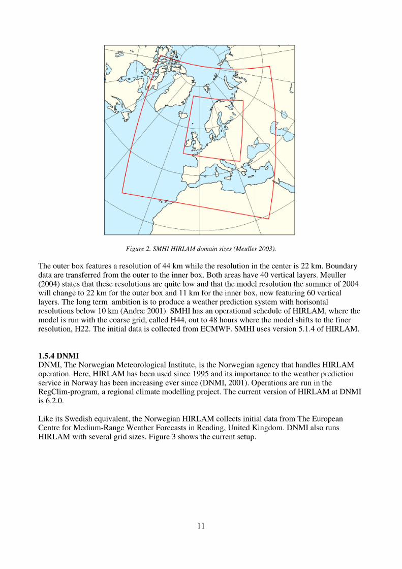
Figure 3. DNMI HIRLAM domain sizes (Vignes 2004).
Currently, three resolutions are used: 0.2°, 0.1° and 0.05°. The number of vertical levels are set to 40 for all of the setups. 1.5.5 Comparison of SMHI and DNMI There are a few differences between the Swedish and Norwegian approaches. Table 2 and 3 show the model domains of HIRLAM setups for each nation.
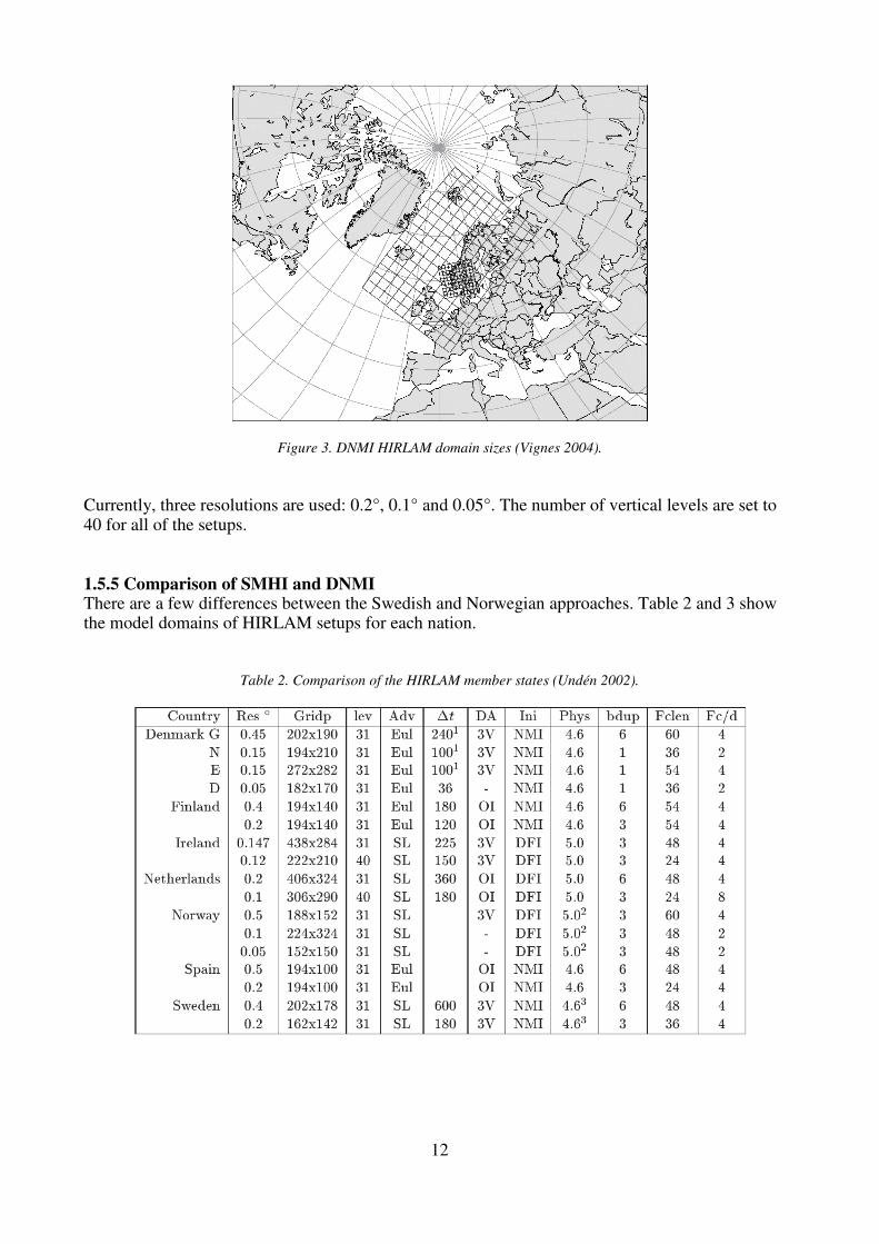
Table 2. Comparison of the HIRLAM member states (Undén 2002).
13
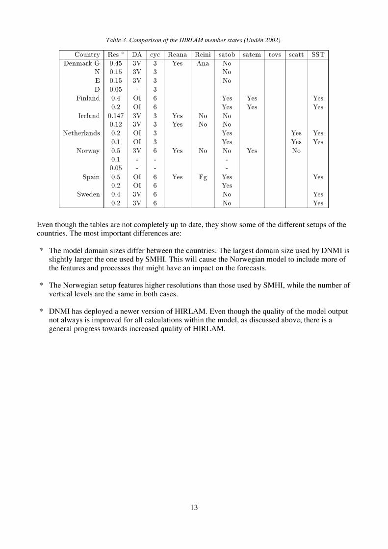
Table 3. Comparison of the HIRLAM member states (Undén 2002).
Even though the tables are not completely up to date, they show some of the different setups of the countries. The most important differences are: * The model domain sizes differ between the countries. The largest domain size used by DNMI is slightly larger the one used by SMHI. This will cause the Norwegian model to include more of the features and processes that might have an impact on the forecasts. * The Norwegian setup features higher resolutions than those used by SMHI, while the number of vertical levels are the same in both cases. * DNMI has deployed a newer version of HIRLAM. Even though the quality of the model output not always is improved for all calculations within the model, as discussed above, there is a general progress towards increased quality of HIRLAM.

14
2 Objectives and scientific questions 2.1 Objectives In this project, weather simulations for the Göteborg region will be performed and studied. The main objectives are: * Implement MeteOS 2002 for the Göteborg region * Test the model setup and examine the impact of different domain sizes and model resolution A MeteOS 2002 installation will be set up and run with a few sets of configurations. This will test the system performance and quality of the model output.
2.2 Scientific questions The scientific questions of this paper are: * How can the model domain size be optimized for the chosen area? * How will a set of different model resolutions affect the model output? The relative importance of model domain will be examined. Also, the effect of resolution on model performance will be analyzed. By using different resolutions, the effect of different processes might influence model output. There are many features that require a relatively fine resolution, in the order of kilometres, for example the land and sea breeze and the influence of the complex topography with its marine influence and the valleys around Göteborg.
15
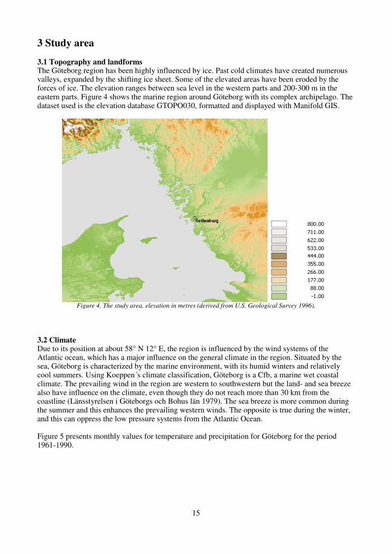
3 Study area 3.1 Topography and landforms The Göteborg region has been highly influenced by ice. Past cold climates have created numerous valleys, expanded by the shifting ice sheet. Some of the elevated areas have been eroded by the forces of ice. The elevation ranges between sea level in the western parts and 200-300 m in the eastern parts. Figure 4 shows the marine region around Göteborg with its complex archipelago. The dataset used is the elevation database GTOPO030, formatted and displayed with Manifold GIS.
Figure 4. The study area, elevation in metres (derived from U.S. Geological Survey 1996).
3.2 Climate Due to its position at about 58° N 12° E, the region is influenced by the wind systems of the Atlantic ocean, which has a major influence on the general climate in the region. Situated by the sea, Göteborg is characterized by the marine environment, with its humid winters and relatively cool summers. Using Koeppen´s climate classification, Göteborg is a Cfb, a marine wet coastal climate. The prevailing wind in the region are western to southwestern but the land- and sea breeze also have influence on the climate, even though they do not reach more than 30 km from the coastline (Länsstyrelsen i Göteborgs och Bohus län 1979). The sea breeze is more common during the summer and this enhances the prevailing western winds. The opposite is true during the winter, and this can oppress the low pressure systems from the Atlantic Ocean. Figure 5 presents monthly values for temperature and precipitation for Göteborg for the period 1961-1990.

16
Temperature and precipitation 1961-1990
-5
0
5
10
15
20
Jan Feb Mar Apr May Jun Jul Aug Sept Oct Nov Dec
Month
Te
mpe
ratu
re (
°C)
0
20
40
60
80
100
Jan Feb Mar Apr May Jun Jul Aug Sept Oct Nov Dec
Temperature
T+stdv
T-stdv
Precipitation
Figure 5. Annual temperature and precipitation distribution for Göteborg (derived from Alexandersson et al 2001).
As shown in Figure 5, the monthly mean temperature ranges from just below freezing-point in January to the summer maximum of about 18º in July. The mean annual temperature in the region is 6-8º (Länsstyrelsen i Göteborgs och Bohus län, 1979). Figure 2 also includes data for the standard deviation (stdv) of the temperature , calculated for 1994-2003 (derived from SMHI 1993-2004). This will be of interest for evaluation of the results since this describes to what degree the temperature will vary over the year. For the period used, the standard deviation of the temperature is about 1-2º Celsius. A similar pattern can also be recognized for the precipitation. Maximum occurs late summer and precipitation decreases somewhat during autumn to spring, where the minimum occurs. This precipitation distribution is due to the elevated summer temperatures, which accelerates evaporation and consequently precipitation.

17
4 Data and methods
4.1 MeteOS 2002 and MM5 4.1.1 MM5 The numerical model used with MeteOS 2002 is MM5. MM5, The Fifth-Generation NCAR / Penn State Mesoscale Model, is a nonhydrostatic, limited-area mesoscale meteorological model. Model development was initiated in the early 70's. The MM5 model optionally features multiple resolutions with several nested domains running simultaneously. Like the HIRLAM, there are several external tools for data management, statistical analysis and other fields. Being a mesoscale model, MM5 will require data for the initial and lateral boundary meteorological conditions for the full period (UCAR 2003). Figure 6 shows the basic architecture of the MM5 model.
Figure 6. Visualization of MM5 (UCAR, 2003), reprinted with permission.
The MM5 model has been widely used for research and the model homepage, http://www.mmm.ucar.edu/mm5/mm5-home.html , provides a wide range of references. 4.1.2 MeteOS 2002 For this paper, MeteOS 2002 has been chosen to create weather predictions. This software, developed by Angel Dimitrov at the Storm Laboratory in Varna, Bulgaria, uses the mesoscale model MM5 for meteorological simulations. MeteOS 2002 is highly configurable and the user has a rich set of options for adapting it to the desirable conditions. It is developed for use with Mandrake 8.1, a distribution of the Linux system. MeteOS 2002 is used for purposes such as weather prediction and research. For example, it is currently used by the Storm Laboratory, Bulgaria. MeteOS 2002 was chosen for this project because of its ease of use, ability to run on modest hardware and configurability. The MeteOS project is hosted at http://www.angelfire.com/sc/stormlab/meteos/meteos.html .
18
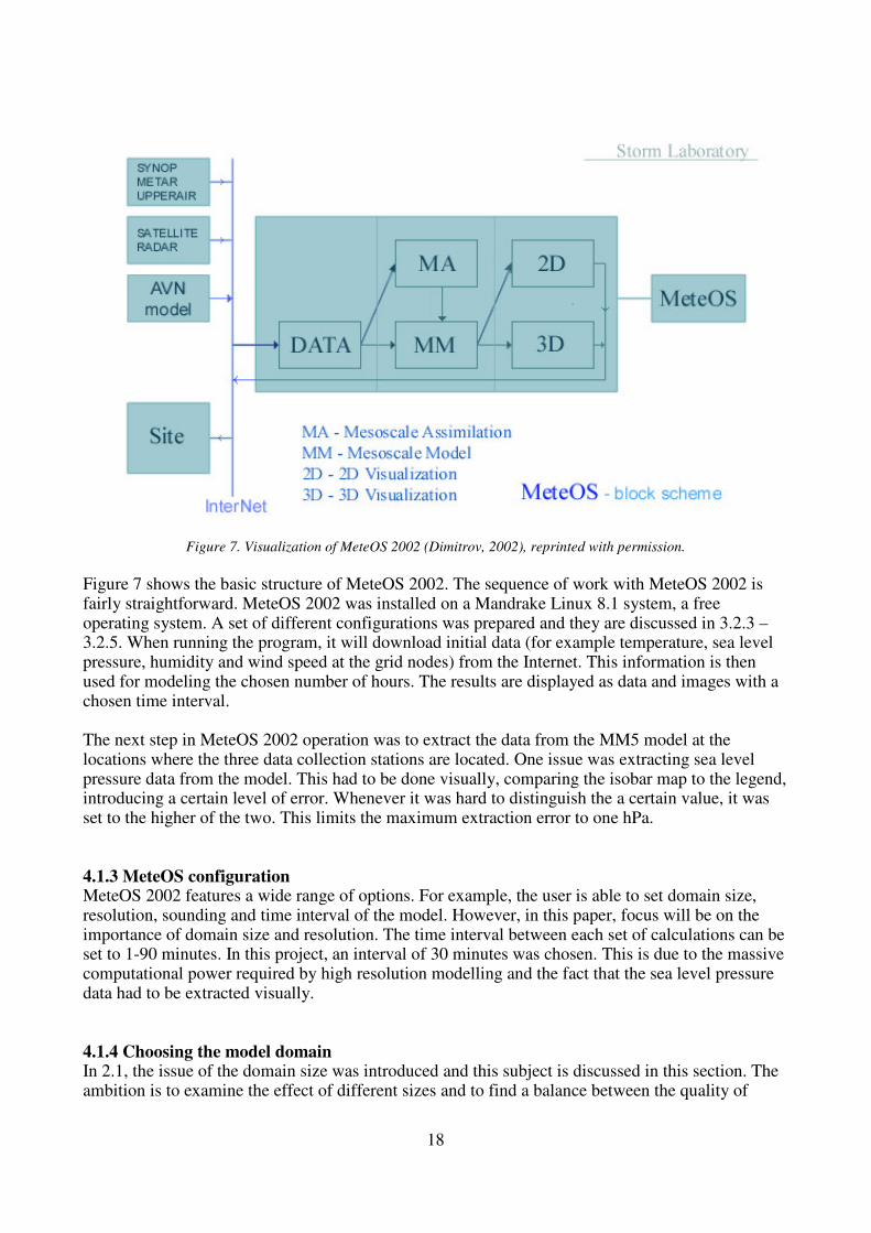
Figure 7. Visualization of MeteOS 2002 (Dimitrov, 2002), reprinted with permission.
Figure 7 shows the basic structure of MeteOS 2002. The sequence of work with MeteOS 2002 is fairly straightforward. MeteOS 2002 was installed on a Mandrake Linux 8.1 system, a free operating system. A set of different configurations was prepared and they are discussed in 3.2.3 – 3.2.5. When running the program, it will download initial data (for example temperature, sea level pressure, humidity and wind speed at the grid nodes) from the Internet. This information is then used for modeling the chosen number of hours. The results are displayed as data and images with a chosen time interval. The next step in MeteOS 2002 operation was to extract the data from the MM5 model at the locations where the three data collection stations are located. One issue was extracting sea level pressure data from the model. This had to be done visually, comparing the isobar map to the legend, introducing a certain level of error. Whenever it was hard to distinguish the a certain value, it was set to the higher of the two. This limits the maximum extraction error to one hPa. 4.1.3 MeteOS configuration MeteOS 2002 features a wide range of options. For example, the user is able to set domain size, resolution, sounding and time interval of the model. However, in this paper, focus will be on the importance of domain size and resolution. The time interval between each set of calculations can be set to 1-90 minutes. In this project, an interval of 30 minutes was chosen. This is due to the massive computational power required by high resolution modelling and the fact that the sea level pressure data had to be extracted visually. 4.1.4 Choosing the model domain In 2.1, the issue of the domain size was introduced and this subject is discussed in this section. The ambition is to examine the effect of different sizes and to find a balance between the quality of

19
model output and performance. If the domain is undersized, the model may be unable to include some of the features that determine the regional climate of the area. Conversely, if it is sized too generously, the amount of data may be overwhelming and hard to analyze. Over sizing the chosen area will also cause problems due to the rather limited computational resources in this project. In order to find the sensitivity of domain, three tests were performed, each with different domain size: 300 x 300, 500 x 500 and 800 x 800 km. These sizes were chosen because they represent a quite wide spectrum of domain sizes, while still not being too large to run with modest hardware. All other parameters, such as model resolution, remained have remained fixed during these tests. The model resolution was set to 15 km for all three model domain tests.
Figure 8. Domain sizes, centered around Gothenburg.
Figure 8 roughly shows the different domain sizes, centered around the Göteborg area. 4.1.5 Choosing the resolution The configuration of MeteOS 2002 will allow resolutions from 1 to 90 km. However, because of the complex physical properties of the Göteborg region, focus will be on high resolutions. Small scale processes and features, such as the land and sea breeze, the maritime influence and land/sea mask are of significant importance to the meteorological conditions in Göteborg. The spatial resolutions selected are 6, 11 and 15 km. This is partly due to the fact that the current resolution of the HIRLAM setup used by SMHI is 11 km. Therefore, it is interesting to study the effect of higher resolution as well as the effects of a coarser resolution. One important issue when discussing simulation is the time of forecast. As discussed by Lorenz

20
(1988), the chaotic nature of the weather system makes high quality long predictions hard to achieve. While MeteOS 2002 allows forecasts for up to 60 hours and in this project, forecasts of 48 hours will be created and analyzed. This is mainly due to the limited computational resources prohibiting extensive modeling and the fact that some of the data had to be extracted visually. 4.1.6 Data collection stations In order to assess how well the MM5 model performs for the chosen conditions, the data will be compared to data from weather stations and statistically analyzed. The chosen stations are located at the airport in Säve, the central parts of Göteborg and Nidingen, respectively. The stations are shown in Figure 9.
Figure 9. Satellite image showing the locations of weather data stations (GLCF 2000), enhanced in Manifold GIS.

21
Table 4. Weather data collection stations
ID Station name Lat Long Elevation (m) Temperature (°C)
Pressure Provider
1 Säve airport 57.78 11.88 53 x x SMHI
2 Skanstorget 57.71 11.99 10 x x Luftnet
3 Nidingen 57.3 11.9 x x SMHI
Figure 9 shows the locations of the meteorological data collection stations. SMHI has a wide range of meteorological stations in Sweden for collecting temperature and precipitation data (Alexandersson 2002). As seen in Table 4, all of the selected stations, except for Nidingen, collects data for temperature and air pressure. SMHI collects temperature data at 1.5 m above ground level. Luftnet, at the environmental administration in Göteborg, collects data from the station in Skanstorget, located a few km from the city center. There are numerous other stations with comparable data but this project uses a total of three stations, which have been selected for their spatial distribution. Data from these stations is collected on an hourly basis by Luftnet for Skanstorget and by SMHI for the stations at Säve and Nidingen every third hour. This enables high resolution data validation. 4.1.7 Test period and data MeteOS 2002 was used for the period 17th - 26th of September 2004 and all of the tests were run twice during this period. One benefit of using this period is the fact that it is relatively even-tempered, avoiding some of the complexity of for example quick winter temperature drops. This is further discussed in 5.3. The collected data shows temperatures around 10-16° C, except for a few short nightly temperature drops. Normal temperatures for this period are around 13° C. The period was generally characterized by low pressure systems from the Atlantic Ocean. These were normally centered to the west of Sweden, around Iceland and Great Britain. 4.1.8 Evaluation of prediction Even though each of the setups discussed in 4.1.4 and 4.1.5 was tested twice during the period, it should be stressed, that the results can not be generalized for a wider field. This is for example due to the characteristics of the Göteborg region. The quality of model output for specific meteorological conditions is also important. Each test should be performed extensively but this is beyond the limitations of this project, see 5.3. Thornes et al. (2001) states that there are several components that contribute to the quality of weather forecasts: reliability, accuracy, skill, resolution, sharpness and uncertainty. It is also mentioned, that no single verification process will provide complete information about the quality of the forecast. There are several approaches for testing the reliability of the data status and it is important to determine the properties of the data. Is it of yes/no nature, for example temperatures below zero?

22
The data in this paper is continuous, i.e. temperature and sea level pressure. WWRP/WGNE (2004) lists several methods for evaluating the quality of the forecast. For example, mean error, multiplicative error and mean absolute error are discussed. In this paper, the root mean square error (RMSE), also discussed by Pielke (2002), will be used.
The formula shown above is the RMSE, which has been calculated for the 24:th and 48:th hour of the forecasts. N is the amount of hours, Fi the forecast and Oi the observed data. Some of the advantages of the RMSE are that this is a commonly known and extensively used method, that is simple to use. However, it does not tell the direction of the errors, i.e. the error is always positive. The statistical analysis also included a bias test, as shown below. This will help any general and continuous differences between the model output and the data collected. For example, if the model continuously overestimates the temperature, this effect can be estimated by using a bias test.
By adjusting for the general error from the model output, the results might be easier to evaluate and any trends easier to identify.
23
5 Results
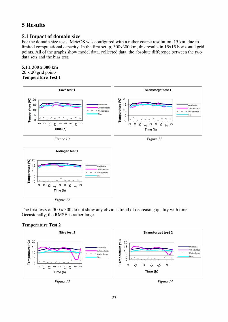
5.1 Impact of domain size For the domain size tests, MeteOS was configured with a rather coarse resolution, 15 km, due to limited computational capacity. In the first setup, 300x300 km, this results in 15x15 horizontal grid points. All of the graphs show model data, collected data, the absolute difference between the two data sets and the bias test. 5.1.1 300 x 300 km 20 x 20 grid points Temperature Test 1
Säve test 1
0
5
10
15
20
3 9
15
21 3 9
15
21 3
Time (h)
Tem
pera
ture
(ºC
)
Model data
Collected data
Mod-collected
Bias
Skanstorget test 1
0
5
10
15
20
3 9
15
21 3 9
15
21 3
Time (h)
Tem
pera
ture
(ºC
)
Model data
Collected data
Mod-collected
Bias
Figure 10 Figure 11
Nidingen test 1
0
5
10
15
20
3 9
15
21 3 9
15
21 3
Time (h)
Tem
pera
ture
(ºC
)
Model data
Collected data
Mod-collected
Bias
Figure 12
The first tests of 300 x 300 do not show any obvious trend of decreasing quality with time. Occasionally, the RMSE is rather large. Temperature Test 2
Säve test 2
0
5
10
15
20
9
15
21 3 9
15
21 3 9
Time (h)
Tem
pera
ture
(ºC
)
Model data
Collected data
Mod-collected
Bias
Skanstorget test 2
0
5
10
15
20
9 18 3 12 21 6
Time (h)
Tem
pera
ture
(ºC
)
Model data
Col lected data
Mod-col lected
Bias
Figure 13 Figure 14
24
Nidingen test 2
0
5
10
15
209
15
21 3 9
15
21 3 9
Time (h)
Tem
pera
ture
(ºC
)
Model data
Collected data
Mod-collected
Bias
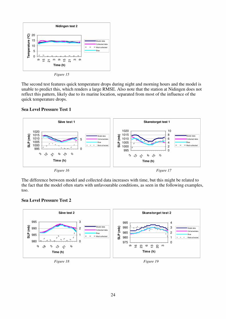
Figure 15
The second test features quick temperature drops during night and morning hours and the model is unable to predict this, which renders a large RMSE. Also note that the station at Nidingen does not reflect this pattern, likely due to its marine location, separated from most of the influence of the quick temperature drops. Sea Level Pressure Test 1
Säve test 1
99510001005101010151020
3 12 21 6 15 0
Time (h)
SL
P (
mb
)
0
5
Model data
Col lected data
Bias
Mod-col lected
Skanstorget test 1
995
1000
1005
1010
1015
1020
3 12 21 6 15 0
Time (h)
SL
P (
mb
)
0
2
4
6
8
10
Model data
Collected data
Bias
Mod-collected
Figure 16 Figure 17
The difference between model and collected data increases with time, but this might be related to the fact that the model often starts with unfavourable conditions, as seen in the following examples, too. Sea Level Pressure Test 2
Säve test 2
980
985
990
995
9 18 3 12 21 6
Time (h)
SL
P (
mb
)
0
1
2
3
Model data
Collected data
Bias
Mod-collected
Skanstorget test 2
975
980
985
990
995
9
16
23 6
13
20 3
Time (h)
SL
P (
mb
)
0
1
2
3
4
Model data
Col lected data
Bias
Mod-col lected
Figure 18 Figure 19

25
5.1.2 500 x 500 km 32 x 32 grid points Temperature Test 1
Säve test 1
0
5
10
15
20
21 3 9
15
21 3 9
15
21
Time (h)
Tem
pera
ture
(ºC
)
Model data
Collected data
Mod-collected
Bias
Skanstorget test 1
0
5
10
15
20
21 3 9 15 21 3 9 15 21
Time (h)
Tem
pera
ture
(ºC
)
Model data
Collected data
Mod-collected
Bias
Figure 20 Figure 21
Nidingen test 1
0
5
10
15
20
21 3 9 15 21 3 9 15 21
Time (h)
Tem
pera
ture
(ºC
)
Model data
Collected data
Mod-collected
Bias
Figure 22
The first test with 500 x 500 km show a quite low RMSE and the temperature is stable. Temperature Test 2
Säve test 2
0
5
10
15
20
21 3 9
15
21 3 9
15
21
Time (h)
Tem
pera
ture
(ºC
)
Model data
Collected data
Mod-collected
Bias
Skanstorget test 2
0
5
10
15
20
21 3 9
15
21 3 9
15
21
Time (h)
Tem
pera
ture
(ºC
)
Model data
Collected data
Mod-collected
Bias
Figure 23 Figure 24

26
Nidingen test 2
0
5
10
15
2021 3 9
15
21 3 9
15
21
Time (h)
Tem
pera
ture
(ºC
)
Model data
Collected data
Mod-collected
Bias
Figure 25
Again, night time temperature drops cause the RMSE to increase to unacceptable levels, since the error exceeds the collected data. While the first test rendered RMSEs of 0-2°C, the second features much larger ones. Sea Level Pressure Test 1
Säve test 1
985990995
1000100510101015
21 3 9 15 21 3 9 15
Time (h)
SL
P (
mb
)
024681012
Model data
Collected data
Bias
Mod-collected
Skanstorget test 1
985990995
1000100510101015
21 3 9 15 21 3 9 15
Time (h)
SL
P (
mb
)
024681012
Model data
Collected data
Bias
Mod-collected
Figure 26 Figure 27
The RMSEs increase with time. The sea level pressure data does not suffer from the same problems that cause the errors when modelling the temperature. Sea Level Pressure Test 2
Säve test 2
983985987989991993995
21 6 15 0 9 18
Time (h)
SL
P (
mb
)
0123456
Model data
Collected data
Bias
Mod-collected
Skanstorget test 2
975
980
985
990
995
21 6 15 0 9 18
Time (h)
SL
P (
mb
)
0
2
4
6
8
Model data
Collected data
Bias
Mod-collected
Figure 28 Figure 29
The two tests show opposite trends, and this could be related to the high input data at Skanstorget.
27
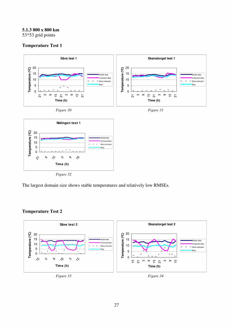
5.1.3 800 x 800 km 53*53 grid points Temperature Test 1
Säve test 1
0
5
10
15
20
21 3 9
15
21 3 9
15
21
Time (h)
Tem
pera
ture
(ºC
)
Model data
Collected data
Mod-collected
Bias
Skanstorget test 1
0
5
10
15
20
21 3 9
15
21 3 9
15
21
Time (h)
Tem
pera
ture
(ºC
)
Model data
Collected data
Mod-collected
Bias
Figure 30 Figure 31
Nidingen test 1
0
5
10
15
20
21 6 15 0 9 18
Time (h)
Tem
pera
ture
(ºC
)
Moded data
Col lected data
Mod-col lected
Bias
Figure 32
The largest domain size shows stable temperatures and relatively low RMSEs. Temperature Test 2
Säve test 2
0
5
10
15
20
15 0 9 18 3 12
Time (h)
Tem
pera
ture
(ºC
)
Model data
Col lected data
Mod-col lected
Bias
Skanstorget test 2
0
5
10
15
20
15
21 3 9
15
21 3 9
15
Time (h)
Tem
pera
ture
(ºC
)
Model data
Collected data
Mod-collected
Bias
Figure 33 Figure 34

28
Nidingen test 2
0
5
10
15
2015
21 3 9
15
21 3 9
15
Time (h)
Tem
pera
ture
(ºC
)
Model data
Collected data
Mod-collected
Bias
Figure 35
Several occasions with low temperatures render high RMSEs. The low RMSEs of Nidingen might be explained by its marine location. Sea Level Pressure Test 1
Säve test 2
970
980
990
1000
1010
1020
21 6 15 0 9 18
Time (h)
SL
P (
mb
)
-1
1
3
5
7
9
Model data
Collected data
Bias
Mod-collected
Skanstorget test 1
970
980
990
1000
1010
1020
21 3 9
15
21 3 9
15
21
Time (h)
SL
P (
mb
)
-1
1
3
5
7
9
Model data
Collected data
Bias
Mod-collected
Figure 36 Figure 37
Figure 36 and 37 show several occasions with poor model output. Sea Level Pressure Test 2
Säve test 2
980
985
990
995
1000
1005
15 0 9 18 3 12
Time (h)
SL
P (
mb
)
0
2
4
6
8
10Model data
Collected data
Bias
Mod-collected
Skanstorget test 2
980
985
990
995
15 0 9 18 3 12
Time (h)
SL
P (
mb
)
0
2
4
6
8
10
Model data
Collected data
Bias
Mod-collected
Figure 38 Figure 39
Figure 38 features a trend with increasingly poor results.

29
5.2 Effect of model resolution 5.2.1 15 km Same as the results from domain size 500 x 500 km. 5.2.2 11 km Temperature Test 1
Säve test 1
0
5
10
15
20
21 3 9
15
21 3 9
15
21
Time (h)
Tem
pera
ture
(ºC
)
Model data
Collected data
Mod-collected
Bias
Skanstorget test 1
0
5
10
15
20
21 3 9
15
21 3 9
15
21
Time (h)
Tem
pera
ture
(ºC
)
Model data
Collected data
Mod-collected
Bias
Figure 40 Figure 41
Nidingen test 1
0
5
10
15
20
1 3 5 7 9 11 13 15 17
Time (h)
Tem
pera
ture
(ºC
)
Model data
Collected data
Mod-collected
Bias
Figure 42
With few exceptions, the 11 x 11 test shows relatively low RMSEs. Temperature Test 2
Säve test 2
0
5
10
15
20
9
15
21 3 9
15
21 3 9
Time (h)
Tem
pera
ture
(ºC
)
Model data
Collected data
Mod-collected
Bias
Skanstorget test 2
0
5
10
15
20
9
15
21 3 9
15
21 3 9
Time (h)
Tem
pera
ture
(ºC
)
Model data
Collected data
Mod-collected
Bias
Figure 43 Figure 44

30
Nidingen test 2
0
5
10
15
20
9 18 3 12 21 6
Time (h)
Tem
pera
ture
(ºC
)
Model data
Col lected data
Mod-col lected
Bias
Figure 45
In the second test, the model is unable to cope with the complex patterns of temperature changes, and this renders large RMSEs. Sea Level Pressure Test 1
Säve
970
980
990
1000
1010
1020
1 3 5 7 9 11131517
Time (h)
SL
P (
mb
)
0
5
10 Model data
Collected data
Bias
Mod-collected
Skanstorget test 1
960970980990
100010101020
21 3 9
15
21 3 9
15
21
Time (h)
SL
P (
mb
)
0
5
10
15
Model data
Collected data
Bias
Mod-collected
Figure 46 Figure 47
The sea level pressure output in figure 48 and 49 is generally poor, with errors up to about 11 mb. Sea Level Pressure Test 2
Säve test 1
970
980
990
1000
1010
9 17 1 9 17 1 9
Time (h)
SL
P (
mb
)
-1
4
9
14
Model data
Col lected data
Bias
Mod-col lected
Skanstorget test 2
970
980
990
1000
1010
9 17 1 9 17 1 9
Time (h)
SL
P (
ºC)
0
2
4
6
8
Model data
Col lected data
Bias
Mod-col lected
Figure 48 Figure 49
The second test of 11x11 km features somewhat smaller errors.

31
5.2.3 6 km Temperature Test 1
Säve test 1
0
5
10
15
20
15
21 3 9
15
21 3 9
15
Time (h)
Tem
pera
ture
(ºC
)
Model data
Collected data
Mod-collected
Bias
Skanstorget test 1
0
5
10
15
20
15
21 3 9
15
21 3 9
15
Time (h)
Tem
pera
ture
(ºC
)
Model data
Collected data
Mod-collected
Bias
Figure 50 Figure 51
Nidingen test 1
0
5
10
15
20
15
21 3 9
15
21 3 9
15
Time (h)
Tem
pera
ture
(ºC
)
Model data
Collected data
Mod-collected
Bias
Figure 52
When testing the 6 x 6 km setup, the model performs very well when the conditions are stable, but the quality is decreased for the Säve and Skanstorget stations. Temperature Test 2
Säve test 2
0
5
10
15
20
15
21 3 9
15
21 3 9
15
Time (h)
Tem
pera
ture
(ºC
)
Model data
Collected data
Mod-collected
Bias
Skanstorget test 2
0
5
10
15
20
15
21 3 9
15
21 3 9
15
Time (h)
Tem
pera
ture
(ºC
)
Model data
Collected data
Mod-collected
Bias
Figure 53 Figure 54

32
Nidingen
0
5
10
15
2015
21 3 9
15
21 3 9
15
Time (h)
Tem
pera
ture
(ºC
)
Model data
Collected data
Mod-collected
Bias
Figure 55
The high RMSEs for some of the stations for the second test indicate that the model, again, is unable to handle quick and large temperature changes. Sea Level Pressure Test 1
Säve test 1
970
980
990
1000
1010
15 0 9 18 3 12
Time (h)
SL
P (
mb
)
-4
1
6
11
16
Model data
Collected data
Bias
Mod-collected
Skanstorget test 1
960970980990
10001010
15 0 9 18 3 12
Time (h)
SL
P (
mb
)
0
5
10
15
Model data
Col lected data
Mod-col lected
Bias
Figure 56 Figure 57
Except for the initial period, the model performs well with the highest resolution. Sea Level Pressure Test 2
Säve test 2
970
980
990
1000
1010
15 0 9 18 3 12
Time (h)
SL
P (
mb
)
-1
4
9
14
Model data
Collected data
Bias
Mod-collected
Skanstorget test 2
970
980
990
1000
1010
15 0 9 18 3 12
Time (h)
SL
P (
mb
)
0
2
4
6
8
Model data
Collected data
Bias
Mod-collected
Figure 58 Figure 59
Here, the model does not forecast the increase of the sea level pressure and this might be related to the equivalent changes in temperature.
33
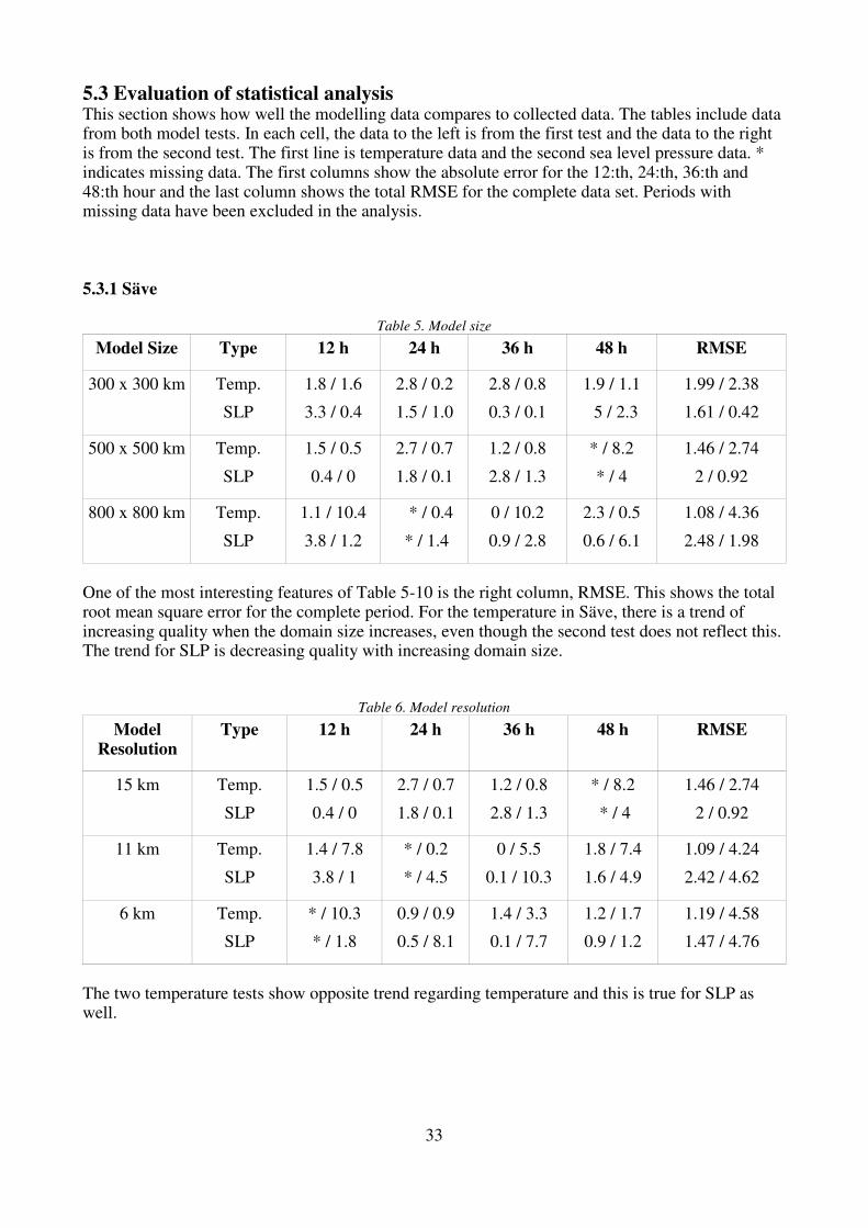
5.3 Evaluation of statistical analysis This section shows how well the modelling data compares to collected data. The tables include data from both model tests. In each cell, the data to the left is from the first test and the data to the right is from the second test. The first line is temperature data and the second sea level pressure data. * indicates missing data. The first columns show the absolute error for the 12:th, 24:th, 36:th and 48:th hour and the last column shows the total RMSE for the complete data set. Periods with missing data have been excluded in the analysis. 5.3.1 Säve
Table 5. Model size
Model Size Type 12 h 24 h 36 h 48 h RMSE
300 x 300 km Temp.
SLP
1.8 / 1.6
3.3 / 0.4
2.8 / 0.2
1.5 / 1.0
2.8 / 0.8
0.3 / 0.1
1.9 / 1.1
5 / 2.3
1.99 / 2.38
1.61 / 0.42
500 x 500 km Temp.
SLP
1.5 / 0.5
0.4 / 0
2.7 / 0.7
1.8 / 0.1
1.2 / 0.8
2.8 / 1.3
* / 8.2
* / 4
1.46 / 2.74
2 / 0.92
800 x 800 km Temp.
SLP
1.1 / 10.4
3.8 / 1.2
* / 0.4
* / 1.4
0 / 10.2
0.9 / 2.8
2.3 / 0.5
0.6 / 6.1
1.08 / 4.36
2.48 / 1.98
One of the most interesting features of Table 5-10 is the right column, RMSE. This shows the total root mean square error for the complete period. For the temperature in Säve, there is a trend of increasing quality when the domain size increases, even though the second test does not reflect this. The trend for SLP is decreasing quality with increasing domain size.
Table 6. Model resolution
Model Resolution
Type 12 h 24 h 36 h 48 h RMSE
15 km Temp.
SLP
1.5 / 0.5
0.4 / 0
2.7 / 0.7
1.8 / 0.1
1.2 / 0.8
2.8 / 1.3
* / 8.2
* / 4
1.46 / 2.74
2 / 0.92
11 km Temp.
SLP
1.4 / 7.8
3.8 / 1
* / 0.2
* / 4.5
0 / 5.5
0.1 / 10.3
1.8 / 7.4
1.6 / 4.9
1.09 / 4.24
2.42 / 4.62
6 km Temp.
SLP
* / 10.3
* / 1.8
0.9 / 0.9
0.5 / 8.1
1.4 / 3.3
0.1 / 7.7
1.2 / 1.7
0.9 / 1.2
1.19 / 4.58
1.47 / 4.76
The two temperature tests show opposite trend regarding temperature and this is true for SLP as well.

34
5.3.2 Skanstorget
Table 7. Model size
Model Size Type 12 h 24 h 36 h 48 h RMSE
300 x 300 km Temp.
SLP
0.3 / 0.3
5.3 / 3
1.7 / 0.6
4.2 / 2.6
1.8 / 1.1
4.5 / 2.7
1.7 / 0.1
7.2 / 0.8
1.7 / 2.1
4.6 / 2.8
500 x 500 km Temp.
SLP
1.2 / 0.3
3.5 / 7
1.1 / 0.6
1.3 / 2.6
0.4 / 0.3
5.6 / 0.7
0.4 / 2.8
10.1 / 0.8
0.9 / 1.8
5.1 / 3.4
800 x 800 km Temp.
SLP
0.4 / 6
0.3 / 4.5
0.9 / 1.9
7.4 / 1.2
0.6 / 8.4
0.9 / 2.2
0.5 / 0.2
6.4 / 5.8
0.8 / 3.3
3.4 / 3.6
For the temperature in Skanstorget, the temperature shows opposite trends while the SLP tests are characterized by large RMSEs.
Table 8. Model resolution
Model Resolution
Type 12 h 24 h 36 h 48 h RMSE
15 km Temp.
SLP
1.2 / 0.3
3.5 / 7
1.1 / 0.6
1.3 / 2.6
0.4 / 0.3
5.6 / 0.7
0.4 / 2.8
10.1 / 0.8
0.9 / 1.8
5.1 / 3.4
11 km Temp.
SLP
0.1 / 2.3
6.6 / 2.5
1.3 / 2.1
6.1 / 0.5
0.5 / 0.9
3.4 / 6.1
0 / 3.5
5 / 1.9
0.9 / 2.5
5.3 / 3.3
6 km Temp.
SLP
7.1 / 7.5
1.9 / 2
0.2 / 0.5
2.4 / 4.2
3.5 / 0
3.5 / 4.1
2.6 / 3.7
1.8 / 2.1
3.4 / 3.2
3.6 / 3.1
The impact of model resolution on temperature in Skanstorget is not clear. For SLP, this station features as increasing quality with resolution, while the second test shows the opposite. 5.3.3 Nidingen
Table 9. Model size
Model Size Type 12 h 24 h 36 h 48 h RMSE
300 x 300 km Temp.
SLP
1 / 0.2
*
2.8 / 0.2
*
1.7 / 0.8
*
0.7 / 0.6
*
1.3 / 0.6
* / *
500 x 500 km Temp.
SLP
1 / 0.1
*
1.7 / 1.1
*
0.8 / 0.9
*
0.7 / 0
*
0.8 / 0.5
* / *
35
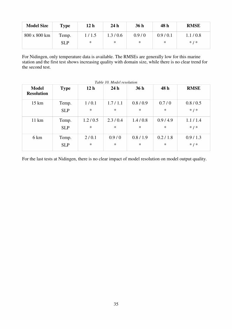
Model Size Type 12 h 24 h 36 h 48 h RMSE
800 x 800 km Temp.
SLP
1 / 1.5
*
1.3 / 0.6
*
0.9 / 0
*
0.9 / 0.1
*
1.1 / 0.8
* / *
For Nidingen, only temperature data is available. The RMSEs are generally low for this marine station and the first test shows increasing quality with domain size, while there is no clear trend for the second test.
Table 10. Model resolution
Model Resolution
Type 12 h 24 h 36 h 48 h RMSE
15 km Temp.
SLP
1 / 0.1
*
1.7 / 1.1
*
0.8 / 0.9
*
0.7 / 0
*
0.8 / 0.5
* / *
11 km Temp.
SLP
1.2 / 0.5
*
2.3 / 0.4
*
1.4 / 0.8
*
0.9 / 4.9
*
1.1 / 1.4
* / *
6 km Temp.
SLP
2 / 0.1
*
0.9 / 0
*
0.8 / 1.9
*
0.2 / 1.8
*
0.9 / 1.3
* / *
For the last tests at Nidingen, there is no clear impact of model resolution on model output quality.

36
6 Discussion
6.1 Impact of domain size 6.1.1 Temperature The general expected results have been decreasing quality of the model output as the prediction advances, as discussed in 1.2 with the older prediction models. Since the introduction of small errors constantly will have an increasing influence on the predictions, this could have negative effect on model output, slightly increasing with each set of calculations. The expected trend of the domain size was decreasing RMSEs with an increasing domain size. Larger models should be able to include more of the meteorological features that have influence on the conditions in the study area. For the station in Säve, the first test showed a decreasing RMSE with an increasing model domain size. The second test showed the opposite trend. This was however associated with large RMSEs, around 10°C, and short temperature drop during the nights, something that was not reflected in the model data. This pattern can be observed for other tests as well; the poor output of some tests coincide with low night time temperatures and the data from tests with low RMSEs feature a more homogenous pattern. The first test from Skanstorget shows a decreasing RMSE with increasing domain size, while the second test contradicts this, even though the trend is diffuse. Since this data collection station is located in the city centre of Göteborg, there are numerous reasons that could help explain these results. This is discussed in 6.3. Data from Nidingen show a equivocal pattern. The first test renders somewhat decreasing RMSEs with increasing model domain, while trend in the second test is uncertain. 6.1.2 Sea Level Pressure The effect of domain size on the RMSE of sea level pressure data was found to be somewhat inconsistent with the expected results. When evaluating data for Säve, it was found that both tests had resulted in increasing RMSEs with increasing domain size. However, this can partly be explained by quick changes in sea level pressure, circumstances where the model performs poorly compared to conditions with stable SLPs. The first test from Skanstorget shows no clear trend. The period was characterized by unstable conditions with highly shifting sea level pressure, which the model seems unable to predict with intact accuracy. The second test shows slightly increasing RMSEs with increasing domain size. This test, too, was associated with somewhat unstable conditions
6.2 Effect of model resolution 6.2.1 Temperature The two tests from Säve each show different behaviour. In the first test, the RMSEs decrease with increasing resolution. The second test points in the opposite way. It should be stressed that this test, as well as many of those that contradict the expected results, feature greater RMSEs for all model output, making the data less reliable. The results from Skanstorget show a general trend of increasing RMSEs with increasing resolution. These tests were generally associated with the unfavourable unstable conditions. Test number one from Nidingen shows no clear trend while the
37
second shows increasing RMSEs with increasing resolution. 6.2.2 Sea Level Pressure The first test from Säve shows that the RMSEs decrease with increasing resolution, even though the trend is not ideal. The second test contradicts this but the RMSEs are high and it is likely that other factors have had major influence here. Both tests from Skanstorget show decreasing RMSEs with increasing resolution, but these tests are associated with relatively high RMSEs, too. In their research, Horritt and Bates (2001) found that model performance of river flooding improved up to a certain resolution, after which no further improvements were found. This is of interest to this paper, since the trend was not clear in some cases. The significance of even higher resolutions might be declining when using MeteOS and MM5, too. Further studies with higher resolutions are required to study this.
6.3 Uncertainties The approach of the weather forecasts in this paper is associated with a number of uncertainties, some of which will be discussed here. These can be divided into two major groups: uncertainties related to the MM5 model and those that are associated with the data collected from the meteorological stations. 6.3.1 Modeling problems Generally, there are two ways of modeling weather forecasts. The first, and preferred method, is running all of the tests for the same period of time, e.g. starting at 15.00 a specific day. Since the weather forecasting process involves calculation of heavy data sets, this requires massive computational power or the capability of storing the initial data and use the same data set for all setups. This was not possible for this project, since using MeteOS 2002 only allows using the current data. The only alternative is therefore running the model several times for each setup and identify the trends that are statistically significant. The simulations of different domain sizes and resolutions were initiated at different stages, which might have influence on the data rendered. It can not be dismissed that the forecasting system is able to achieve improved performance for some meteorological conditions, while others cause increased liability to deviations. Here, each setup has been tested twice but would have benefited from additional model tests in order to find any statistically significant trends. There are issues associated with the modeling itself, as can be seen when choosing different domain size and resolution. As mentioned in 6.1, the output error should increase slightly with each set of calculations due to the imperfect nature of the model. Since the quality of the model output could vary with the meteorological conditions at startup and during the test, it can not be ruled out that the specific conditions during the model tests have had impact on the results. Another important aspect of the modeling problems are the various types of data used by the model. For example, the land use characterization and other surface data used by the model has an influence on the model output. Since the surface of sea and land have distinct properties, the model will perform poorly will incorrect initial conditions.

38
6.3.2 SMHI / Luftnet data The data collected from the weather stations is another source of uncertainty and there are various sources of error associated with this issue. For example, the collected data might be affected by the urban heat island produced in Göteborg. For major cities, this can add some 10°. For Göteborg, this temperature is smaller, around a few degrees. Since the data collection stations are located at different distances from the city centre, the effect of the urban heat island is consequently diversified. The instruments are located at a given height above ground level. Because of the lapse rate and wind turbulence associated with densely developed areas, this might induce invalid data when comparing collected data to model data. Also, since the data is collected at numerous locations with different sets of meteorological equipment, some uncertainty can be related to this issue. For some periods, there was data missing from the data collected by SMHI. This has had a negative effect, since there was no way of validating the model output for these occasions. There are a number of sources for errors, some of which are induced by the presence of man. For example, there are many types of particles present in the atmosphere. Traffic and transportation are considerable sources of particles. As discussed in 1.4, Booij (2004) found a small increase with model resolution, a trend that has been found for some cases in this paper, too. Also, Horritt & Bates (2001) found that the quality of model output does not increase beyond a certain resolution, a result that is supported by this project.

39
7 Conclusions One of the main objectives of this paper has been finding the optimal domain size and MM5 resolution. The main conclusions are: Domain size
• For stable conditions, the quality of the model output increases with increasing domain size in three out of six temperature tests. However, if the occasions with generally large RMSEs are removed, three out of four tests show increased quality. The equivalent trend for sea level pressure is only found in one out of four tests, since relatively large RMSEs had been calculated. This is believed to be because larger domains include more of the meteorological features of the region.
• During unstable conditions with quick changes of temperature and sea level pressure, the model is sometimes unable to make forecasts with preserved quality. Most of the results contradicting the expected trend derive from these conditions. To overcome this, the model should be tested extensively for a wide range of synoptic situations. Model resolution
• Increasing the resolution had a positive impact on the quality of three out of six tests. For sea level pressure, the same was found in two out of four tests.
• Some of the tests suffer from the same problems as the experiments with domain size; unfavourable meteorological conditions complicate the study of the effect of model resolution. It has been shown that the RMSE of this project strongly depends on the synoptic weather situation. At occasions with quick changes in weather, the significance of model domain size and resolution is reduced in the tests performed and no clear trend was found. Further research should therefore test the full synoptic range in order to minimize this effect.
Scientific significance As mentioned in 1.1, there are several sectors that could benefit from the results of meteorological modelling. The main aim of this paper is to discuss and analyze the use of MM5 and MeteOS 2002, hence, it is important to consider the scientific value of the project. What is the importance of these tests? How can the conclusions contribute to further understanding of the meteorological modelling? Firstly, the results show that the model still has problems with quick changes in weather. Additional resources should be focused on fine tuning the MM5 model on these issues. As the model development advances and becomes more user friendly (as the case is when using it with MeteOS), it should be more widely accepted by the general public, enabling an enhanced user base, making user defined and local weather forecasts available. All of the sectors mentioned in 1.1 should benefit from this development, provided it is combined with a quality assessment system, such as the one used in this paper.

40
The information rendered in this project is valuable for understanding weather and climate in general and for Göteborg in particular. The effect of domain size and model resolution could help identify the dominant processes that are important to the regional climate. This is also essential when developing weather forecasting systems. Knowing the most important processes will provide guidance for further development.
41
References Alexandersson H (2002): Temperatur och nederbörd i Sverige 1860-2001, SMHI Alexandersson H & Eggertsson C (2001): Temperaturen och nederbörden i Sverige 1961-1990, Referensnormaler - utgåva 2, SMHI, 88p Andræ U (2001): High resolution modeling at SMHI, SMHI, 8 p Boiij M (2004): Impact of climate change on river flooding assessed with different spatial model resolutions, Journal of Hydrology, p 176-198 Dimitrov A: (2002): MeteOS 2002 Meteorological Operation System User´s Manual, http://www.angelfire.com/sc/stormlab/meteos/doc/readme.txt Dimitrov A (2002): MM5 Model [Mesoscale and Microscale Modeling Division] Advanced User´s Manual, http://www.angelfire.com/sc/stormlab/meteos/doc/mm5_help.txt DNMI (2001): HIRLAM – Blinderns ukjente arbeidshest, http://met.no/p_og_t/marked/vermelding/mai_2001_7.html Dudhia J, Gill D, Manning K, Wang W & Bruyere (2004): PSU/UNCAR Mesoscale Modeling System Tutorial Class Notes and Users´ Guide (MM5 Modeling System Version 3), http://www.mmm.ucar.edu/mm5/documents/tutorial-v3-notes.html European Centre for Medium-Range Weather Forecasts (2002): The early history of Numerical Weather Prediction, http://www.ecmwf.int/products/forecasts/guide/The_early_history_of_Numerical_Weather_Prediction.html Global Land Cover Facility (2000): Landsat ETM+, NASA, http://glcf.umiacs.umd.edu/index.shtml Graham S, Parkinson C & Chahine M (2001): Weather Forecasting Through the Ages, NASA Earth Observatory, http://earthobservatory.nasa.gov/Library/WxForecasting/ HIRLAM management team: The Reference System, HIRLAM, http://hirlam.knmi.nl/open/reference.htm Holton J (2002): Dynamic Meteorology, Third Edition, Academic Press, 511 p Horritt M & Bates P (2001): Effects of Spatial resolution on a model of flood flow, Journal of Hydrology 253, p 239-249 Lorenz E (1989): Computational Chaos – A prelude to computational instability, Physica D 35, p 299-317 Länsstyrelsen i Göteborgs och Bohus Län (1979): Natur i Göteborgs och Bohus län, 288 p Meuller L (2004): SHMI operational HIRLAM system, Madrid, 2004, 5 p O´Connor J & Robertson E (2003): Lewis Fry Richardson, University of St Andrews, http://www-gap.dcs.st-and.ac.uk/~history/Mathematicians/Richardson.html

42
O´Connor J & Robertson E (2003): Vilhelm Frimann Koren Bjerknes, University of St Andrews, http://www-gap.dcs.st-and.ac.uk/~history/Mathematicians/Bjerknes_Vilhelm.html Pielke R (2002): Mesoscale Meteorological Modeling, Second Edition, International Geophysics Series Volume 78, 676 p SMHI (1993-2004), Väder och Vatten, SMHI Thornes J & Stephenson D (2001): How to judge the quality and value of weather forecast products, Meteorol Appl 8, p 307-314 UCAR (2003): MM5 Modelling System Overview, http://www.mmm.ucar.edu/mm5/overview.html Undén P, Rontu L, Järvinen H, Lynch P, Calvo J, Cats G, Cuxart J, Eerola K, Fortelius C, Garcia-Moya J, Jones C, Lenderlink G, McDonald A, McGrath R, Navascues B, Nielsen N, Ødegaard V, Rodriguez E, Rummukainen M, Rõõm R, Sattler K, Sass B, Savijärvi H, Schreur B, Sigg R, The H & Tijm A (2002): HIRLAM-5 Scientific Documentation, SMHI, 146 p U.S. Geological Survey (1996): GTOPO30, http://edcdaac.usgs.gov/gtopo30/gtopo30.asp Vignes O (2004): Operational NWP at met.no, DNMI, 4 p WWRP/WGNE Joint Working Group on Verification (2004): Forecast Verification - Issues, Methods and FAQ, http://www.bom.gov.au/bmrc/wefor/staff/eee/verif/verif_web_page.html